Galactic Edge Clouds I:
Molecular Line Observations and
Chemical Modelling of Edge Cloud 2

Abstract

Edge Cloud 2 (EC2) is a molecular cloud, about 35 pc in size, with one of the largest galactocentric distances known to exist in the Milky Way. We present observations of a peak CO emission region in the cloud and use these to determine its physical characteristics. We calculate a gas temperature of 20 K and a density of $n(\mathrm{H}_{2})\sim 10^{4}$ cm^-3. Based on our CO maps, we estimate the mass of EC2 at around $10^{4}\,M_{\sun}$ and continuum observations suggest a dust-to-gas mass ratio as low as 0.001. Chemical models have been developed to reproduce the abundances in EC2 and they indicate that: heavy element abundances may be reduced by a factor of five relative to the solar neighbourhood (similar to dwarf irregular galaxies and damped Lyman alpha systems); very low extinction ($A_{\mathrm{V}}<4$ mag) due to a very low dust-to-gas ratio; an enhanced cosmic ray ionisation rate; and a higher UV field compared to local interstellar values. The reduced abundances may be attributed to the low level of star formation in this region and are probably also related to the continuing infall of primordial (or low metallicity) halo gas since the Milky Way formed. Finally, we note that shocks from the old supernova remnant GSH 138–01–94 may have determined the morphology and dynamics of EC2.

1 Introduction

Observations of CO emission at large galactocentric distances have detected a number of molecular clouds, among which is Edge Cloud 2 (hereafter EC2), with an estimated kinematic galactocentric distance of $R\sim 28$ kpc (Digel et al., 1994). Although this kinematic distance for the far-outer Galaxy should be treated with caution, EC2 appeared to be up to 6 kpc further away than Edge Cloud 1 (EC1), the next most distant molecular cloud detected by Digel et al., and much further than the extent of the optical disk of the Milky Way, $\sim$ 15–19 kpc (Fich et al., 1989; Robin et al., 1992). This is almost as far as the most distant H i, detected at $\sim$ 30 kpc (Kulkarni et al., 1982). More recently Levine et al. (2006) have traced the spiral structure in the southern half of the Galaxy out to at least 25 kpc, implying a minimum radius for the gas disk. EC2 has an effective radius of $\sim$20 pc and is situated $\sim$350 pc below the distant warped Galactic plane (Digel et al., 1996b). The CO luminosity of EC2 is at least a factor of 2 larger than those of the other 10 clouds detected at large distances, and is comparable to that of the Taurus Giant Molecular Cloud (Digel et al., 1994). EC2 is also the only edge cloud detected in the high-density tracer CS (Digel et al., 1996a). The CO maps of EC2 show that it has sub-structure. It is in a region of extremely low gas pressure and very small spiral arm perturbation.

EC2 was also found to have an associated H ii region excited by an early B star (MR1) (de Geus et al., 1993) that appears to have triggered star formation. Studies of metallicity as a function of galactocentric distance have shown that there is a galactic metallicity gradient. Spectra of MR1 (Smartt et al., 1996) indicate significant metal depletion – with elemental abundances reduced on average by some 0.5 dex – and that its galactocentric distance is more likely to be in the range 15-19 kpc (placing it at the limit of the optical disk). Subsequently, Rolleston et al. (2000) have calculated metal depletions of about five for C, N, and O. Kobayashi & Tokunaga (2000) used NIR observations to argue that MR1 has triggered the formation of young stellar objects in EC2. Snell et al. (2002) argue that it is the most distant cloud in the Milky Way, with evidence for massive star formation, although this distinction is claimed for WB89-789 by Brand & Wouterloot (2007). More recently, two embedded young star clusters have been associated with EC2 (Kobayashi et al., 2005). Yasui et al. (2006) identified 52 members in one of the clusters, suggesting that the cluster is a T Tauri association. Stil & Irwin (2001) associate EC2 with the approaching side of the H i shell from supernova remnant (SNR) GSH 138–01–94, thereby setting the galactocentric distance $R\sim 23.6$ kpc for EC2. Because of the uncertainty of $R$ for EC2, we have used two heliocentric distances, 14 and 20 kpc ($R=22$ and 28 kpc) for any distance sensitive calculations in this work.

Current models of galacto-chemical evolution include time and spatial variations in the halo gas infall and star formation rate whereby the Galactic halo, bulge, and thick disk formed first, separately from the thin disk, in two infall episodes. Chemical abundances of the interstellar medium and their radial variation across galactic disks provide a fundamental set of constraints for theories of disk formation and evolution. The most accepted mechanism to explain the existence of abundance gradients in disk galaxies is the so-called ‘biased-infall’ (Chiappini & Matteucci, 1999), where infall of gas occurs at a faster rate in the innermost regions than in the outermost ones (‘inside-out’ disk formation). Growing observational evidence for slow formation of disks in spiral galaxies associated with continuing infall of primordial (or low metallicity) gas over the lifetime of the disk (e.g. Braun & Burton, 1999) seems to give support to the above scenario. Lubowich et al. (2000) demonstrated that continuous infall of low-metallicity gas is occurring in the Galactic Center.

Of particular relevance to test these models are the abundances in the very outer galactic disks. Chemical evolution models for abundance gradients and the formation of the Milky Way (Chiappini et al., 2001) show that the steepness of the outer gradients are particularly sensitive to thresholds in star formation, to the halo-thick disk enrichment history, and to the radial variation of the disk formation timescales. They concluded that some abundance ratios increase substantially toward the outermost disk regions but that ‘more observations at large galactocentric distances are needed to test these predictions’. The fact that N is almost constant with the galactocentric distance up to 18 kpc (Chiappini et al., 2003) reflects the high N production in AGB stars. The primary N contribution from AGB stars is however very uncertain. At such large galactocentric distances a N production threshold may be operating due to the paucity of late-type stars.

Galactic chemical evolution also predicts that the abundances of C, N, O, ¹³C, and ¹⁵N will be lower in clouds at the edge of the Galaxy than in any other cloud of the Galactic disk (Maciel & Quireza, 1999). The composition of these edge clouds should be similar to that of the early Galactic disk modified by infall from the halo. Thus the metallicity in clouds such as EC2 is expected to be similar to dwarf irregular galaxies, giving us an unique opportunity to study gas from the early stages of the formation of the Galactic disk (Kobayashi & Tokunaga, 2000).

We have, therefore, searched for emission from a number of molecules towards EC2, concentrating on the northern CO peak (which is coincident with the T Tauri cluster identified by Yasui et al., 2006), in order to constrain its physical conditions and chemical composition. Such molecular evolution in low metallicity Galactic clouds also provides a local laboratory in understanding molecular gas in extragalactic sources such as high-$z$ quasars. In particular, since deuterated molecules are sensitive tracers of physical conditions and chemical pathways, we have also searched for a number of deuterium (D) bearing molecules, noting that Rogers et al. (2005) have detected Di towards the Galactic anticenter. We also examine the role of SNR GSH 138–01–94 in providing the energy input for both the chemistry and star formation observed in EC2.

2 Observations

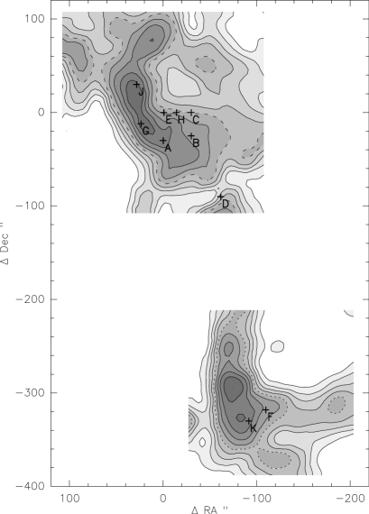
Figure 1: JCMT 15m May-July 2005 combined contour map of observed CO 2–1 intensities, showing observed positions A through K. Positions A, J and K correspond to positions copk1, copk2 and copk3 respectively from Digel et al. (1994). Axis offsets in arcsec from position E ($\alpha_{2000}=$ 02:48:38.5, $\delta=$ 58:28:58.3, $v_{\mathrm{rad}}=-103.70$ km s^-1). EC2MAP1 (top) CO 2–1: peak $T^{*}_{\mathrm{R}}$ = 6.906 K, rms = 0.321 K. EC2MAP2 (bottom) CO 2–1: peak $T^{*}_{\mathrm{R}}$ = 7.124 K, rms = 0.22 K.

We have completed over 210 hours of observations toward this object using the 12 m Arizona Radio Observatory (ARO) telescope (formerly part of the National Radio Astronomy Observatory), the 100 m Max-Planck-Institut für Radioastronomie (MPIfR) Effelsberg telescope, the 15 m James Clerk Maxwell Telescope (JCMT), and the 30 m Institut de Radio Astronomie Millimétrique (IRAM) telescope. The line observations range in frequency from 4.83 GHz (H₂CO 1_1,0–1_1,1) to 492 GHz (Ci ³P₁–³P₀). EC2 is extended in CO and we have observed a number of different positions within $\sim$40″ of the three peaks seen in it by Digel et al. (1994). Fig. 1 shows observed positions A through K on our contour map of CO 2–1 emission. Positions A, J and K correspond to positions copk1, copk2 and copk3 respectively from Digel et al. (1994). In this work we present the results of our line search at position A ($\alpha_{\rm 2000}=02^{\mathrm{h}}\,48^{\mathrm{m}}\,38.5^{\mathrm{s}}$, $\delta_{\rm 2000}=58\arcdeg\,28\arcmin\,28.1\arcsec$), which at the time showed the strongest line spectrum based on a twelve position HCO⁺ map. Our subsequent CO maps centered on position E, ($\alpha_{\rm 2000}=02^{\mathrm{h}}\,48^{\mathrm{m}}\,38.5^{\mathrm{s}}$, $\delta_{\rm 2000}=58\arcdeg\,28\arcmin\,58.3\arcsec$), covering the northern peak in emission, are also presented. These maps revealed that the northern peak in CO emission was $\sim$30″ north-east of position A, and $\sim$25% stronger. See Lubowich et al. (2004) for observations of positions B and C. Full details of observed line spectra for positions other than A, and CO maps covering the southern peak (centered at $\alpha_{\rm 2000}=02^{\mathrm{h}}\,48^{\mathrm{m}}\,23.6^{\mathrm{s}}$, $\delta_{\rm 2000}=58\arcdeg\,23\arcmin\,59.0\arcsec$) are available in Ruffle (2006).

Observations at the ARO 12 m were made between June 2002 and January 2006 at 2 and 3 mm. Data were obtained in beam switching mode. The beam size ($\theta_{\mathrm{b}}$) of the 12 m telescope varies between 93″ at 72 GHz and 43″ at 150 GHz. Observing conditions were generally good, with system temperatures ranging from 140 to 350 K for the 2002 June observations. For subsequent observations, system temperatures ranged from 170 to 820 K. Dual channel SIS receivers were used in conjunction with two spectrometer systems: Filter Banks 1 and 2 (FB1 and FB2), and a digital Millimeter Auto Correlator (MAC1). The 256 channel 100 and 250 kHz filter bank spectrometers were used simultaneously, with 128 channels allocated to each polarisation, giving bandwidths of 12.8 and 32 MHz respectively. The two polarisations were subsequently averaged during data reduction. The MAC1 was used to confirm filter bank data and set to a resolution of 50, 100, 200 or 400 kHz and bandwidths of 300 or 600 MHz. The ARO 12 m produces spectral line data calibrated to the $T^{*}_{\mathrm{R}}$ (K) corrected antenna temperature scale.

We used the Effelsberg 100 m telescope in June 2002, December 2002, January 2003, May 2004 and November 2005 at 1.0, 1.3, 2, and 6 cm to observe transitions of SO, NH₃, H₂O, and H₂CO with beamwidths ($\theta_{\mathrm{b}}$) of about 30^′′, 40^′′, 55^′′′ and 160^′′ and typical system temperatures of 400, 150, 80, and 40 K on a main beam brightness temperature scale ($T_{\rm mb}$). $T_{\rm mb}$ to flux density conversion ratios were 1.6, 1.4, 1.8, and 2.4 K/Jy, respectively. For the 1.0 cm SO 1₀–0₁ line and the 2 cm H₂CO 2_1,1–2_1,2 transition, single channel primary focus HEMT (High Electron Mobility Transistor) receivers were employed. At 1.3 cm, for H₂O and NH₃, a primary focus dual channel HEMT receiver was used, allowing us to add signals with orthogonal linear polarization, thus reducing the effective system temperature given above by $\sim$30%. At 6 cm, H₂CO 1_1,0–1_1,1 observations were taken with a four channel secondary focus receiver. Position switching with appropriate offsets, alternating between east and west in azimuth, was used for all measurements. An ‘AK90’ autocorrelator included four spectrometers with 2048 channels and bandwidths of 20 MHz each. Pointing was accurate to about 10″ or better.

In June 2004–July 2005, we used the JCMT to map the 2–1 and 3–2 transitions of several isotopes of CO and to observe the 492 GHz transition of Ci with beam sizes ($\theta_{\mathrm{b}}$) which range from 23″ at 220 GHz to 10″ at 492 GHz. We also searched unsuccessfully for the HCO⁺ 3–2 transition at 267 GHz. Data were obtained in a position-switching mode in a tracking coordinate frame with a chop throw of 600″ at an angle of 270°. For the CO 2–1 and HCO⁺ observations, the single channel A3 receiver was used yielding system temperatures from 260–330 K. For the CO 3–2 transitions the dual channel B3 receiver was used with two low-noise SIS mixers in single-sideband mode, yielding system temperatures from 420–800 K. Receiver W was used to observe the Ci transition in single sideband with a system temperature of 2400–4100 K. The JCMT produces spectral line data calibrated to the $T^{*}_{\mathrm{A}}$ (K) antenna temperature scale, and this was converted to $T^{*}_{\mathrm{R}}$ using the JCMT’s $\eta_{\mathrm{fss}}$ (forward scattering and spillover) efficiencies.

Finally, in October-November 2005 we used the MAMBO II bolometer at the IRAM 30 m telescope to make a 1.2 mm dust emission map of EC2. The bolometer comprises 117 pixels with a resolution of 11″. Zenith opacity ranged from 0.07–0.27 during the observations and the sky noise difference (between on and off source) was generally low, varying between 34 and 90 mJy/beam/2 Hz. We made five maps of EC2 centered on $\alpha_{2000}$=02:48:41.0, $\delta_{2000}$=58:29:27.9, with an rms which ranged from 8.8–11.5 mJy per beam. The five maps were combined using MOPSIC.

3 Analysis

Detected lines, CO maps, dust maps and a summary of observations can be found in Figs. 1 through 7 and Table 1.

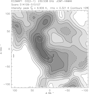
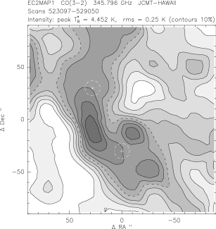
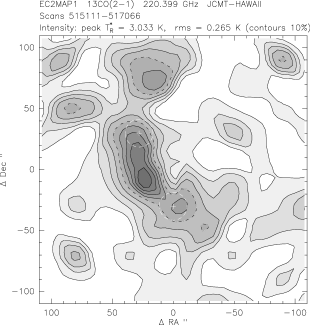
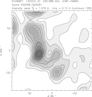
Figure 5: JCMT 15 m May-July 2005 maps of observed CO intensities centered on position E ($\alpha_{2000}=$ 02:48:38.5, $\delta=$ 58:28:58.3, $v_{\mathrm{rad}}=-103.70$ km s^-1) with position A ($\alpha_{2000}=$ 02:48:38.5, $\delta=$ 58:28:28.1) 30″ below map center. Axis offsets in arcsec, contour levels 10% of peak, dashed contours 50% of peak (FWHP) and white circle is half-power beam width (HPBW). (a) CO 2–1: peak $T^{*}_{\mathrm{R}}$ = 6.906 K, rms = 0.321 K. (b) CO 3–2: peak $T^{*}_{\mathrm{R}}$ = 4.452 K, rms = 0.25 K. (c) ¹³CO 2–1: peak $T^{*}_{\mathrm{R}}$ = 3.033 K, rms = 0.265 K. (d) ¹³CO 3–2: peak $T^{*}_{\mathrm{R}}$ = 1.579 K, rms = 0.12 K.

Before estimating abundances of the observed molecular species, we first have to determine the main physical parameters of the gas, i.e. its density and temperature, taking into account the beam-filling by deconvolving the detected intensities. To estimate the latter we use the ¹²CO and ¹³CO 2–1 maps in Fig. 5 and assume that the source, which has an elongated shell-like structure, has a full-width at half power ($fwhp$) size of $150\arcsec\times 40\arcsec$ ($\theta_{\mathrm{s}}\equiv 77\arcsec$) for ¹²CO, and $100\arcsec\times 30\arcsec$ ($\theta_{\mathrm{s}}\equiv 55\arcsec$) for ¹³CO, C¹⁸O and all other molecules. The peak intensities listed in Table 1 are corrected for these source sizes using $T_{\mathrm{mb}}=T^{*}_{\mathrm{R}}/\eta_{\mathrm{bf}}$, with $\eta_{\mathrm{bf}}=\theta^{2}_{\mathrm{s}}/(\theta^{2}_{\mathrm{s}}+\theta^{2}_{\mathrm{b}})$, where $\eta_{\mathrm{bf}}$ is the beam filling correction factor.

There are several tracers sensitive to both density and temperature, though none that only traces density, but one that exclusively traces kinetic temperature. The species allowing us to determine $T_{\mathrm{kin}}$ is NH₃.

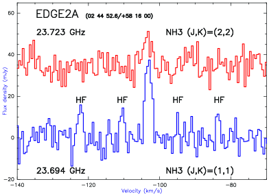
Figure 2: EC2 spectra observed at the MPIfR Effelsberg 100 m position A: (top) NH₃ (J,K) = (1,1) and (2,2) (HF = group of satellite hyperfine components). (middle) H₂CO 2_1,1–2_1,2 and 1_1,0–1_1,1. Note that the scale for the 2_1,1–2_1,2 transition has been multiplied by 5. (bottom) SO 1₀–0₁.

We have detected at least four of the five groups of hyperfine components in the ($J,K$)=(1,1) line of NH₃ (see Fig. 2, the satellite features being marked ‘HF’). Line intensity ratios are consistent with optically thin emission. Gaussian fits of the groups of hyperfine components are (with increasing velocity) 23.3, 17.2, 80.2, 5.7 and 11.1 mJy km s^-1. For the (2,2) line we get 38.0$\pm$8.0 mJy km s^-1. The (2,2)/(1,1) line intensity ratio is then 0.28$\pm$0.07, with the error being dominated by the low signal-to-noise ratio of the (2,2) line. To derive total beam-averaged column densities in an inversion doublet, we use

$$N(J,K)=1.55\times 10^{14}\frac{J(J+1)}{\nu\,K^{2}}\int{T_{\mathrm{mb}}\mathrm{d}V}$$ (1)

(e.g. eq. 1 in Henkel et al., 2000) that is valid in the optically thin limit. The column density $N$, the frequency $\nu$, and the integral are in units of cm^-2, GHz, and K km s^-1, respectively. As already indicated in section 2, the conversion factor between the Jy and the $T_{\mathrm{mb}}$ scale is 1.6. Thus we obtain total beam averaged column densities of 2.52 $\times$ 10¹² and 5.21 $\times$ 10¹¹ cm^-2 in the (1,1) and (2,2) inversion doublets. The (2,2)/(1,1) column density ratio is then 0.21$\pm$0.05. With

$$N(2,2)/N(1,1)=(5/3)e^{-\Delta E/kT}$$ (2)

and $\Delta E/k=40.957$ K, the difference in energy between the (1,1) and (2,2) levels, we derive a rotational temperature $T=20\pm 3$ K.

With the also populated inversion singlet (0,0) level at 23.19 K below the (1,1) state, the total NH₃ column density, summed over the (0,0), (1,1) and (2,2) levels is $N$(NH₃) = 5.77 $\times$ 10¹² cm^-2, with an uncertainty of $\pm$15 per cent, averaged over the 40″ beam. $J>K$ levels require extremely high densities (Mauersberger et al., 1985) and are therefore not relevant.

Using this rotational temperature, which should be close to the kinetic temperature (Walmsley & Ungerechts, 1983; Danby et al., 1988), the density of EC2 was estimated using Large Velocity Gradient (LVG) models for a number of molecular species, for a spherical cloud with constant density (see Henkel et al., 1980; Mauersberger et al., 1990, and references therein). The results from these models are included in Table 2. First, we use a LVG model involving 40 ortho-H₂CO states up to $K_{\mathrm{a}}=3$ and the collision cross sections of Green (1991). We find that the observed deconvolved line intensities for both the cm and mm lines are well reproduced with a density $n(\mathrm{H}_{2})=1.2\times 10^{4}$ cm^-3. Second we fit the ¹³CO and C¹⁸O spectra to an LVG model using collisional rates from Flower (2001) and an adopted ortho-para ratio of 3 for H₂, although the results are only weakly dependent on this. We first fitted the three ¹³CO deconvolved lines to derive a density of $n(\mathrm{H}_{2})=3.2\times 10^{3}$ cm^-3. With this density, C¹⁸O (only two lines) and ¹²CO could then also be fitted. This gives isotopical abundances of approximately 100:10:1 for ¹²CO:¹³CO:C¹⁸O (see below). This can not reflect the actual isotopic abundance ratios, as the optically thin ¹²C/¹³C ratio is $\sim$89 in the solar system and 60 to 70 in local diffuse clouds (Wilson & Rood, 1994). Using $n_{\mathrm{lvg}}$(X)/$n$(H₂) from Table 2, the best fit also gives a fractional abundance with regard to H₂ of $\sim$10^-7 for ¹³CO, well below the value of $2\times 10^{-6}$ typically found in local metal-rich molecular clouds. For the C¹⁸O/H₂ ratio the model gives $\sim$10^-8 compared to the local value of $1.7\times 10^{-7}$ with ¹⁶O/¹⁸O = 500 (Frerking et al., 1982).

For the rotational HCN 1–0 transition, our detected hyperfine structure is compatible with optically thin emission, implying that other lines should also be optically thin (HCN 1–0 is among the optically thickest 3 mm lines after CO). Therefore, we have computed LVG models for several other species, and start with those for which we have measured more than one transition. For SO, using the collisional rates of Green (1994), we can fit the $1_{0}$–$0_{1}$ and $3_{2}$–$2_{1}$ lines simultaneously, but only with $n(\mathrm{H}_{2})=1.4\times 10^{5}$ cm^-3, an order of magnitude larger than that derived from H₂CO and two orders of magnitude higher than that obtained from ¹³CO, implying the presence of small-scale clumping. The CS 2–1 and 3–2 deconvolved line temperatures can be roughly fitted (using collisional rates from Turner et al., 1992) with the density of $1.2\times 10^{4}$ cm^-3 obtained for H₂CO. The model reproduces HCO⁺ 1–0 deconvolved line temperatures for both the H₂CO and the SO densities (using collisional rates from Flower, 1999). The HCO⁺ model line intensities appear to be consistent with the observed $J$ = 3–2 upper limit, at least in the case of the lower density of $1.2\times 10^{4}$ cm^-3. For HCN 1–0 we summed the deconvolved integrated intensities of the three hyperfine components and then divided by the average of the line widths to get a peak intensity. Using collisional rates from Schöier et al. (2005), this peak deconvolved line intensity was fitted for both the H₂CO and the SO densities ($1.2\times 10^{4}$ cm^-3 and $1.4\times 10^{5}$ cm^-3 respectively). The higher density model is likely to be the correct one; as in the case of HCN, radio observations are mainly sensitive to high density gas. The model reproduces HNC deconvolved line temperatures for both the H₂CO and SO densities (using rates from Schöier et al., 2005). N₂H⁺ was not detected, which is highly unusual and presumably a sign of N depletion.

There are several ways to explain the discrepancies between the expected and derived from observations ¹²CO:¹³CO:C¹⁸O abundance ratios, and the surprisingly low fractional abundances of ¹³CO and C¹⁸O: (i) optical thickness of ¹²CO; (ii) ¹³CO enhancement by fractionation in cloud edges due to charge exchange reactions with C⁺ (e.g. Watson et al., 1976); or (iii) small scale clumping, suggested by the H₂ density derived from the SO line intensity ratio. The energy barrier for the fractionation reaction ${}^{13}\mathrm{C}^{+}+\,^{12}\mathrm{CO}\,\longleftrightarrow\,^{13}\mathrm{CO}+\,^{12}\mathrm{C}^{+}$ is $\sim$35 K (Watson et al., 1976), which requires low temperatures for efficient fractionation, although at 20 K the enhancement would not be large. Low $A_{\mathrm{V}}$ and a high UV field are also required for the production of C⁺. However, for higher UV fields, since ¹²CO self-shields more effectively than ¹³CO, selective photodissociation destroys ¹³CO faster than ¹²CO. So depending on the respective rates of the fractionation reaction and photodissociation, ¹³CO fractionation may or may not be taking place. Given the range of densities derived, small-scale structure and optical depths effects are the most likely explanations for the discrepancies (section 5 examines the effect of high UV fields and low $A_{\mathrm{V}}$ in greater detail).

In order to derive accurate molecular abundances one needs multiple transitions of a variety of isotopes to account for optical depth and excitation effects. Furthermore, the use of optically thin transitions of isotopes to derive accurate abundances of the main species is also fraught with difficulty since the underlying isotopic ratios may be different in this gas at the edge of the Galaxy than in the more local molecular clouds. To derive molecular abundances for species other than CO, H₂CO and NH₃, we have assumed LTE and an excitation temperature of 20 K. Most of the derived abundances are not very sensitive to temperature, typically varying by less than $\pm$10 per cent for $T=20\pm 3$ K, except for the abundances derived for CO 3–2 ($\pm$22%), Ci ($\pm$18%), SO ($\pm$13%), H₂CO ($\pm$12%) and NH₃($\pm$12%).

For optically thin line emission from linear molecules, we find that the total column density, $N$ (cm^-2), of a molecule with normalised electric dipole moment $\tilde{\mu}$ (in units of 10^-18 esu) with an excitation temperature $T_{\mathrm{ex}}$ emitting at frequency $\nu$ in a transition J$\rightarrow$J–1 can be written in the form:

$$N=\frac{1.603\times 10^{13}}{\tilde{\mu}^{2}}\frac{T_{\mathrm{ex}}}{T_{0}^{2}}e^{(J+1)T_{0}/2T_{\mathrm{ex}}}\int{T_{\mathrm{mb}}\mathrm{d}V},$$ (3)

where $T_{0}=h\nu/k$ and the deconvolved integrated intensity for a Gaussian line profile is given by $1.06\,T_{\mathrm{mb}}\Delta V$ in units of K km s^-1. For non-detections we use the 3$\sigma$ upper limits for the integrated intensity:

$$\Delta(\mathrm{K\,km\,s}^{-1})=3\,rms_{\mathrm{mb}}(1+\alpha)\sqrt{\Delta\nu\Delta V},$$ (4)

where $\alpha$ is the calibration uncertainty taken to be 0.15, $\Delta\nu$ and $\Delta V$ are the spectral resolution and expected line-width (2 km s^-1 is adopted here), both measured in km s^-1. For optically thin emission, the fractional abundance varies proportionally to the integrated line intensity. For CN we summed the intensities of our two observed hyperfine components and adopted a relative intensity of 0.456 to determine the integrated intensity and, thus, $N$(CN). For HCN the sum of the three hyperfine components was used, while for C₂H we used the strongest hyperfine component at 87.317 GHz and adopted a relative intensity of 0.4167.

We take a slightly different approach for SO, which has a ${}^{3}\Sigma$ ground state. We calculate $N$(SO) directly using the formula given by Takano et al. (1995) with the partition function from the JPL Molecular Spectroscopy Catalogue (Pickett et al., 1998). For Ci we use a similar approach to that of Tauber et al. (1995). To estimate $N$(H₂CO) we use the LVG modelled density: $N(\mathrm{H}_{2}\mathrm{CO})=n(\mathrm{H}_{2}\mathrm{CO})\times 1\mathrm{pc}\times\Delta V$, where $n$(H₂CO) is the best fit abundance to the LVG calculation ($1.4\times 10^{-6}$ cm^-3) and $\Delta V=1.3$ km s^-1 (the $1_{1,0}-1_{1,1}$ line is widened by hyperfine structure). Table 1 lists the derived column densities.

Table 2 compares line temperatures and column densities for EC2 derived from our LVG models and observed deconvolved integrated intensities, and it can be seen that in most cases there is good agreement between $N_{\mathrm{mb}}$(X) and $N_{\mathrm{lvg}}$(X). The LVG column densities were calculated from the best fit model densities with $N_{\mathrm{lvg}}$(X) = $n_{\mathrm{lvg}}$(X) $\times$ 1 pc $\times$ $\Delta V$. It should be pointed out that our assumption that $T_{\mathrm{ex}}=T_{\mathrm{kin}}=20$ K could be considered unrealistic, since excitation temperatures are crucial for abundance determination. CO is almost certainly thermalised, but other molecular species may not be thermalised with similar certainty. At the low densities we have derived from the observations, molecules like HCO⁺, HCN and HNC would not be thermalised. However, our LVG results provide a realistic estimate of the real excitation temperature ($T_{\mathrm{ex}}$ in Table 2) for a range of our detected molecules. Recalculating with these specific values (instead of $T_{\mathrm{ex}}=20$ K), gives column densities that only differ by factors of between 0.5 and 3.7 (except CS 3–2 by 8.2).

To aid comparison with local molecular clouds, we have derived molecular abundances relative to that of HCO⁺, assuming that the 1–0 transition is optically thin. Our upper limit to H¹³CO⁺ gives a lower limit to the ¹²C/¹³C ratio of around 17, much less than the lower limit of 201$\pm$15 derived from CO 1–0 by Wouterloot & Brand (1996) towards WB 89-437 at a galactocentric distance of 16.4 kpc, although we note that the value they derive from the 2–1 transition is much smaller, 104$\pm$60. Table 3 shows the result and also the equivalent abundance ratio for the nearby dark clouds L134N (center position), TMC-1 (average), and the range of values derived in L134N (Dickens et al., 2000; Pratap et al., 1997). Note that these authors use isotopic species to determine the column densities of optically thick lines. In particular, they adopt ¹²C/¹³C = 64 for determining the column densities of HCO⁺, HCN and HNC and ¹⁶O/¹⁸O = 500 to determine the CO and ¹³CO column densities. Finally we note that they used a dipole moment of 4.07 D for HCO⁺ compared to the value of 3.9 D used here. Use of our value would increase their abundance ratios by about 10%. Table 3 also gives fractional abundances relative to molecular hydrogen using $N$(H₂) = $7.4\times 10^{22}$ cm^-2 and compares these values with those for the translucent clouds observed by Turner (2000).

Dust emission can be used to estimate the mass of cold molecular clouds and we use our detected peak continuum emission at 1.2 mm to calculate the opacity and dust-to-gas ratio in EC2. First, we estimate $\tau_{\nu}$, the dust opacity at frequency $\nu$, using

$$\tau_{\nu}=B(\nu)/\pi(\theta_{\mathrm{b}}/2)^{2}B_{\nu}(T_{\mathrm{dust}}),\>(\tau\ll 1)$$ (5)

from Hildebrand (1983), where $B_{\nu}(T_{\mathrm{dust}})$ is the Planck function, $T_{\mathrm{dust}}=20$ K, the observed dust emission $B(\nu)=20.3\times 10^{-3}$ Jy, and the beam size $\theta_{\mathrm{b}}=11\arcsec$, which gives a value of $\tau_{\nu}=3.25\times 10^{-4}$. The dust opacity per unit mass column density at frequency $\nu$, is given by $\kappa_{\nu}=3Q_{\nu}/4a\rho$, where $Q_{\nu}$ is the dust emissivity which varies as $\nu^{\beta}$ [$B(\nu)\propto\nu^{\beta}B_{\nu}(T_{\mathrm{dust}})$], the average dust grain radius $a=0.1\,\mu$m, and the density of the dust $\rho=3$ g cm^-3. Values for $Q_{\nu}$, $a$ and $\rho$ are taken from Hildebrand (1983). From Whittet (1992, p150) we note the relation $\rho_{\mathrm{dust}}=\tau_{\nu}/\kappa_{\nu}L$, and it therefore follows that the dust to gas ratio is:

$$\frac{M_{\mathrm{dust}}}{M_{\mathrm{gas}}}=\frac{\tau_{\nu}}{\kappa_{\nu}L\,n(\mathrm{H}_{2})\mu m_{\mathrm{H}}},$$ (6)

where $L=D\theta_{\mathrm{b}}$ is the size of the source and $D$ is the heliocentric distance (14–20 kpc). Table 4 lists derived dust to gas ratios for $D$ = 14 and 20 kpc and a range of values for $\beta$ from 1 to 2 (taken to characterise dust grains that range from amorphous to crystalline), as well as appropriate values for $Q_{1200}$ and $\kappa_{\nu}$.

It now remains to relate the dust to gas ratio to possible values of extinction in EC2. For the standard dust-to-gas mass ratio of 0.01 in the local ISM, it is found that $N(\mathrm{H})/E(B-V)=5.8\times 10^{21}$ atoms cm^-2 mag^-1 (Bohlin et al., 1978) and with $R_{\mathrm{V}}=A_{\mathrm{V}}/E(B-V)$, we can write:

$$A_{\mathrm{V}}=\frac{2n(\mathrm{H}_{2})LR_{\mathrm{V}}}{5.8\times 10^{21}}\>\frac{M_{\mathrm{dust}}/M_{\mathrm{gas}}}{0.01}.$$ (7)

As discussed in Ruffle et al. (2004), the value of $R_{\mathrm{V}}$ may be lower in certain regions of the ISM, so we calculate values of $A_{\mathrm{V}}$ for $R_{\mathrm{V}}=3.1$ and $R_{\mathrm{V}}=2.0$ at the position of maximum continuum emission. As our CO maps show, EC2 is clumpy in structure and the peak dust detection of 20.3 mJy/beam ($\theta_{\mathrm{b}}=11\arcsec$) traces the peak CO emission of one such clump. Over the map, the rms value of 6.35 mJy/beam is $\sim$3 times less than the peak, so extinction in EC2 as a whole is likely to be correspondingly lower.

Finally, we estimate upper and lower limits for the mass of EC2 based on a density of $n(\mathrm{H}_{2})=1.2\times 10^{4}$ cm^-3. From our maps of the two CO 2–1 peaks in EC2 (Fig. 1) we estimate that the cloud consists of two dense clumps $\sim$75″ in diameter, which yield a mass range of $9.3\times 10^{4}$ to $2.7\times 10^{5}\,M_{\sun}$ for the distance range 14–20 kpc. Taking the clumpy structure of EC2 into account, the average density may be of the order $n(\mathrm{H}_{2})=10^{3}$ cm^-3, so our mass estimate is $M_{\mathrm{EC2}}\sim 10^{4}\,M_{\sun}$ (based on their CO detections Digel et al. (1994) estimated $M_{\mathrm{EC2}}=3.7\times 10^{4}\,M_{\sun}$). This value can be compared with a virial mass estimate using the method of MacLaren et al. (1988, equation 3), $M_{\mathrm{vir}}/M_{\sun}=k_{2}r\Delta V^{2}$, where $k_{2}=190$ (for $\rho\propto 1/r$), $r$ is the radius of the clumps in pc, and $\Delta V$ is the ¹³CO line width (FWHM) in km s^-1. MacLaren et al. argue that the virial theorem will only yield a meaningful result if the estimate of $\Delta V$ is found from the average throughout the whole volume of the cloud, including central core regions. An optically thick line such as ¹²CO will only probe the cloud to the surface where the optical depth is unity. On the other hand, an optically thin line, such as ¹³CO should allow sampling of velocities throughout the central, denser regions of the cloud. However, taking the “radius” of EC2 from the ¹²CO observations should avoid the effect of excluding the lower density outer regions, i.e. an overestimation of the total mass. For the distance range 14–20 kpc, the radius of each of the two clumps, $r$ is 2.5–3.7 pc and the line width for the strongest ¹³CO 2–1 transition is 1.87 km s^-1, which yields a total virial mass $M_{\mathrm{vir}}$ = 3.3–4.9 $\times 10^{3}\,M_{\sun}$, somewhat less than our direct estimate above. The lower virial mass suggests that the cloud is gravitationally unstable and a likely site of star formation as suggested by Yasui et al. (2006).

4 Discussion

The data in Table 3 indicate some interesting differences between molecular abundances relative to HCO⁺ in EC2 and local dark molecular clouds. In particular sulfur-bearing molecules, (CS, SO), appear to be very over-abundant; the nitrogen-bearing species HCN is comparable while HNC appears to be marginally under-abundant – the HNC/HCN ratio is less than one, whereas in dark clouds it is usually close to or slightly greater than one – and the radicals CN and C₂H are very much over-abundant. The latter result is typical of photon-dominated regions in which photoprocesses ensure that radicals exist in high abundance. At first glance it would appear that the molecular clouds at the edge of the Galaxy would be less likely to show the effects of PDR chemistry; certainly the flux of UV photons must be much less at the Galactic edge than in the local ISM. However, the critical parameter for determining whether or not photons dominate chemistry is the ratio of UV flux to grain surface area, particularly the area of the small grains which extinguish UV photons most efficiently. At large galactocentric radii, the metal abundances relative to hydrogen are expected to be much reduced, consistent with a reduced dust-to-gas ratio, as discussed previously. In addition, although the region of EC2 appears to contain young T Tauri stars (Yasui et al., 2006), there is no evidence of the late-type stars which produce dust grains.

5 Chemical Modelling

To investigate the properties of EC2 and to see whether it is typical of material which has been less processed, we have made a pseudo-time-dependent chemical kinetic model. This uses observationally derived temperatures and densities and varies elemental abundances, photon flux, cosmic ray ionisation (CRI) rate and gas-to-dust ratio in an attempt to fit the observed results. Chemical reaction rates were taken from Rate99: The UMIST database for astrochemistry (Le Teuff et al., 2000).

Unless otherwise stated, the model assumes $T_{\mathrm{kin}}$ = 20 K, $n$(H₂) = $1.2\times 10^{4}$ cm^-3, based on NH₃, H₂CO, and CO observations, and uses the initial elemental abundances listed in Table 5. For the metals (C, N, O, S, Si and Fe) these are reduced by a factor of five from those typically used for local ISM clouds; we find that without this reduction in elemental abundances, agreement with observations is worsened for $A_{\mathrm{V}}>1$ mag. We have investigated varying the CRI rate and the visual extinction ($A_{\mathrm{V}}$) in order to try and find the best fit to the observations. We also varied the UV photon field, initial abundances, and, specifically, the abundances of sulfur or nitrogen.

Our JCMT CO maps probed at higher resolution (15-23″), but the bulk of our detections (with the ARO 12 m) covered beams of 42-70″. Our Effelsberg detections had beams of 30″ for SO, 40″ for NH₃, and 55″ and 160″ for H₂CO. As described in section 3, our detected peak intensities were deconvolved for these beam sizes ($\theta_{\mathrm{b}}$) and our estimated $fwhp$ clump size ($\theta_{\mathrm{s}}$). The peak CO 2–1 emission seen in our maps is within $\sim$30″, or half a typical beamwidth, of position A. Our ARO 12m detections of CO, CS, SO, HCO⁺, HCN, C₂H and C₃H₂ at nearby positions B, C, D, E, G, H and J (Ruffle, 2006) are commensurate with their position A detections, given that the intensity contours seen in Fig. 1 would be ‘smeared’ by the relevant beam sizes (55-70″). At a distance of 20 kpc, a 60″ beam subtends a linear distance of about 6 pc or a column density of about $2\times 10^{23}$ cm^-2 for $n$(H₂) = $1.2\times 10^{4}$ cm^-3. Since our CO maps show that EC2 is extended and clumpy, the ‘one-point’ model adopted is simplistic; nevertheless, given the lack of data on very small scales, one might hope that the model helps constrain some of the global parameters in the cloud in a ‘beam-averaged’ sense. 321 models with varying parameters were run and the results of testing each one against our observations are detailed in Ruffle (2006).

To test the agreement between each model and our observations, we looked at the ratio of the observed abundance relative to H₂ from Table 3 to the model prediction (or the inverse of that ratio if it was greater than 1) for that species. For each molecule/transition we then square its agreement factor and sum these squares for each model, normalising to get a ‘Fit’ number between 0 and 1. This should be closest to 1 for the model which agrees best. In the case of our multiple transition detections of ¹²CO, ¹³CO and C¹⁸O, we have used a $\sigma$ weighted mean of each isotopomer’s observed column densities, where $\sigma=T_{\mathrm{mb}}/rms_{\mathrm{mb}}$. However, as the models only consider the main isotope of an atom (with the exception of H and D) we have assumed that the isotopic ratios have their local interstellar values (¹²C/¹³C = 60, C¹⁶O/C¹⁸O = 500) and factored our observed (mean) abundances relative to $N$(H₂) accordingly. For the ¹³CO and C¹⁸O transitions, this gives us a reasonably consistent value of $N$(CO)/$N$(H₂) $\sim 1.4\times 10^{-6}$, although the main ¹²CO lines give a value closer to $10^{-7}$. Since the main lines of ¹²CO are optically thick (0.6-2.2 from Table 2), the ratios derived from observation are lower limits.

We have selected 10 models for detailed examination, which can be compared in Tables 6, 7, 8 and 9. We investigated the agreement factor at steady state which for our choice of parameters is reached, in general, at times less than than 10⁵ yr. Fig. 8 plots 3D parameter surfaces of these test results for various combinations of the models, where two parameters are varied and the others are kept constant. For ease of comparison, numbered disks, marked on the 3D plots, indicate the examined models relative to the parameter surfaces. Fig. 9 shows fractional abundances varying over time for five of the models.

Varying CRI and $A_{\mathrm{V}}$

We investigated the agreement tests for values of $A_{\mathrm{V}}$ between 0.5 and 10 mag and a CRI rate between 0.5 and 30 times the standard interstellar rate of $1.3\times 10^{-17}$ s^-1. The UV field was set to the local ISM value. Although many of the models give very similar results, the agreement factor is highest for a CRI rate above 10 $\times$ the ISM value and an $A_{\mathrm{V}}$ of 1 mag. Fig. 8a shows the general trend of varying $A_{\mathrm{V}}$ and CRI. It can be seen that increasing the CRI rate beyond 20 $\times$ the ISM value extends agreement in the model to $A_{\mathrm{V}}$ = 2 mag. What is striking however, is the failure of the model for values of $A_{\mathrm{V}}$ above 2 mag. It should be noted that model results for $A_{\mathrm{V}}\leq 0.5$ mag should be treated with caution, as the model may fail for such low values of $A_{\mathrm{V}}$, since it does not treat the self-shielding of H₂ and CO accurately.

Table 7 shows how well these models actually agree with the observations for four selected models (1–4). Model 1 uses ‘standard’ ISM values for the $A_{\mathrm{V}}$ and CRI rate, Model 2 is the best fit model (CRI = $2.6\times 10^{-16}$ s^-1, $A_{\mathrm{V}}$ = 1 mag), while Model 3 uses CRI = $1.3\times 10^{-16}$ s^-1 and $A_{\mathrm{V}}$ = 2 mag, to illustrate some effects which arise from changing these parameters. Model 4 is the same as Model 3, but with a UV field 10 times the local rate.

For Model 1 the predicted CO/H₂ ratio is 1 order of magnitude higher than all the observations. Models 2 and 4 agree within a factor of 2 for ¹²CO but underestimate ¹³CO and C¹⁸O by $\sim$1 order of magnitude, whereas Model 3 reverses those agreements. Model 1 does badly at reproducing the observed value for atomic C, since when the $A_{\mathrm{V}}$ is 10 mag the cloud is shielded from UV radiation and the bulk of the carbon becomes incorporated into CO. When the $A_{\mathrm{V}}$ is lowered and/or the CRI rate increased, however, CO can be broken down, so that the abundance of Ci remains significant even at steady-state. We find that an $A_{\mathrm{V}}$ of 1 or 2 mag gives a better agreement with the EC2 observation of $N$(C)/$N$(H₂).

The predicted value of C₂H/H₂ in Model 1 agrees with the observations to within a factor of 2, while the other three Models are 10 to 40 times too high. Conversely, Models 1 and 3 over-predict the CN/H₂ ratio by over 2 orders of magnitude, with Models 2 and 4 over-estimating it by 40 and 50 times respectively. The time-dependent results show that Models 2 and 4 have good agreement overall once $t$ is greater than about 2000 yr, whereas neither Model 1 or 3 show good agreement beyond the first 500 years (see Fig. 9f).

Varying UV photon field, CRI and $A_{\mathrm{V}}$

We have also looked at the effect of varying the photon field in the models. Fig. 8b,c shows agreement factors for models with varying $A_{\mathrm{V}}$ and CRI for (b) a UV field increased by a factor of 10 compared to the local ISM value, and (c) a UV field reduced by a factor of 10. It can be seen that a higher UV field improves agreement up to an $A_{\mathrm{V}}$ of 2 mag regardless of CRI rate (although for CRI 20 $\times$ this is extended to 3 mag), with Model 4 the best fit. A lower UV field produces very poor agreement (e.g. Model 5).

Fig. 8d plots fit results from models where the CRI rate is fixed at 20 times the standard value, $A_{\mathrm{V}}$ is varied, and the UV field is varied from one-tenth to 80 times the local interstellar field. As expected, an increase in the UV photon field extends agreement to higher values of $A_{\mathrm{V}}$ (4 mag for 80 $\times$ UV). Table 8 shows the agreement for three of these models. Interestingly, 20 $\times$ UV produces a good fit for atomic carbon at an $A_{\mathrm{V}}$ of 1 mag (Model 6), whereas 40 $\times$ UV at an $A_{\mathrm{V}}$ of 3 mag gives a good fit for CO (Model 7). At steady-state CO is primarily destroyed by photons (only if the UV field is strong enough, or the $A_{\mathrm{V}}$ low enough) or by He⁺ and H${}_{3}^{+}$, whose abundances increase with increasing CRI rate. Again a UV field below the local value produces very poor general agreement, but apart from very high UV fields ($\sim$70 $\times$) at an $A_{\mathrm{V}}$ of $\sim$4 mag, there is poor agreement for any $A_{\mathrm{V}}$ above 3 mag. Interestingly the high UV (20 $\times$) Model 6 shows remarkable agreement from the earliest times and Model 7 (40 $\times$ UV) agrees well from $t=2\times 10^{4}$ yr.

The observed upper limit to the DCO⁺/HCO⁺ ratio, 0.08, is not a useful limit since all models with the exception of Model 1, satisfy this constraint. For C₂H/H₂ and CN/H₂, the ratios are overestimated by 2 orders of magnitude in the low UV Model 5, but the fit improves with increasing UV field, with good agreement reached at 20 $\times$ UV (Model 6). Finally, we note that there is a much better fit to the ammonia abundance in low UV Model 5 (which is also achieved for NH₃ in Model 3 with UV = 1 and CRI = 10 times the local ISM rates).

Varying initial abundances and $A_{\mathrm{V}}$

Initial elemental abundances (see Table 5) were varied between local ISM values and 10 per cent of those values. The parameter surface in Fig. 8e shows that for $A_{\mathrm{V}}$ above 1 mag, the agreement worsens appreciably for initial abundances (IA) above 20 per cent of local cloud values. Table 9 compares Models 8–10, and for IA = 0.1 (Model 8) there is good agreement, except for atomic C and CN ($\sim$1 order of magnitude too great), NH₃ ($\sim$1 order to little), and SO (underestimated by 5 orders). Model 8’s agreement varies considerably in the first 10,000 years or so, before settling down at a steady-state below Model 2 (IA = 0.2).

The observed CS(2–1)/H₂ ratio is fairly well matched by our best fit Models 2 and 4 and very well matched by Models 7 and 8 (UV = 40 and IA = 0.1 respectively). Except for Model 1, though, the predictions for SO are too low by several orders of magnitude. Therefore, we tested the effect of increasing the initial abundance of sulfur relative to other initial abundances (which are set at 20 per cent of local cloud values). As expected the abundances of sulfur-bearing molecules scale linearly with any change in the initial abundance of S. For the N-bearing species, all models except 1 give good agreement for HC₃N and N₂H⁺, but the derived abundances are upper limits, so this result must be treated with some caution. For HCN and HNC the picture is less clear, but abundances are again well matched for our best fit Models 2 and 4. Models 3 and 5 are in good agreement with the NH₃/H₂ ratio, while all other models (except Model 1) predict ratios 2 to 5 orders of magnitude too low. For CN the high UV Model 6 agrees with the observed abundance.

Varying $n(\mathrm{H}_{2})$ and $A_{\mathrm{V}}$

Fig. 8f shows the effect of varying $n(\mathrm{H}_{2})$ and $A_{\mathrm{V}}$ with a UV field set to the local ISM value and a CRI rate 20 times the local ISM value. Densities above $n(\mathrm{H}_{2})=1.2\times 10^{4}$ cm^-3 produce a marked fall-off in agreement. We also found that, even for a UV field 10 times the local interstellar value, the visual extinction must be below $A_{\mathrm{V}}=3$ mag for reasonable agreement.

Deuteration

We failed to detect any deuterated species in this survey, with the upper limits being: DCO⁺/HCO⁺ $<$ 0.08; DCN/HCN $<$ 1.5; C₂D/C₂H $<$ 0.06 and HDCO/H₂CO $<$ 0.01. The models presented here use the underlying D/H ratio from the local ISM. Model 1 predicts DCO⁺/HCO⁺ $\sim$0.25, which is higher than that seen in local dark clouds such as TMC-1, a result of the lower abundance of heavy elements. Models 2 and 4, however, predict very low DCO⁺/HCO⁺ ratios ($\sim$10^-3), whereas Model 3 predicts $\sim$10^-2. The large upper limits on DCN/HCN and C₂D/C₂H mean that these are not useful in constraining the models. Likewise for HDCO and DCO⁺ the fractionation ratios agree except for Model 1.

Fractional abundances over time

To this point our model results have been discussed in terms of steady-state abundances and it is pertinent to ask whether there might be any significant difference if we consider the time-dependent results. Fig. 9 plots the fractional abundances over time for Models 2, 4, 6, 7 and 8. For our best-fit model, Model 2, steady-state is reached very quickly, after around 5,000 years (apart from some slight changes in HCN and HCO⁺). Depending on the choice of the UV field and visual extinction, other models reach steady state on somewhat shorter ($\sim$500 yr, Model 6) or somewhat longer ($\sim 10^{4}$ yr, Model 7) times. The longest time to reach steady state is $\sim$5 10⁴ yr (Model 8) which has the lowest initial elemental abundances. Given that the likely age of the EC2 molecular cloud is greater than a few thousand years, we expect that the steady-state results can be used to compare with the observed abundances.

6 Conclusions

In order to deduce its physical and chemical properties, we have observed continuum emission and a large number of molecular transitions in EC2 at the Galactic edge. We have also made CO maps of EC2 and used these to calculate deconvolved line intensities. A temperature of 20 K was estimated from hyperfine detections of ammonia and a gas density of $n(\mathrm{H}_{2})\sim 10^{4}$ cm^-3 was determined by comparing LVG models of a number of species to their deconvolved line detections. Molecular abundances were also determined from the LVG models and found to be in good agreement with abundances calculated directly from the deconvolved line intensities. From the peak continuum emission we calculated a dust mass for EC2 $\geq 150\,M_{\sun}$ and a dust-to-gas mass ratio $\geq 0.001$.

Through the use of chemical models we have been able to establish the most likely chemical and physical properties of EC2 (although we note that not all observed abundances can be reproduced in a self-consistent manner - see Table 6 where our chemical model agreement results are ranked by fit). There is an indication that heavy elements may be depleted by about a factor of five relative to local molecular clouds (similar to those in dwarf irregular galaxies and damped Lyman alpha systems). Such reduced abundances may be attributed to the low level of star formation in this region and are probably also related to the continuing infall of primordial (or low metallicity) halo gas since the Milky Way formed. The models also suggest a high UV photon field in EC2 (10–20 $\times$ local values), where an increased UV field allows for values of $A_{\mathrm{V}}$ up to 4 mag, especially if this increased field is combined with an increase in CRI (10–20 $\times$), although the models are less sensitive to increases in the CRI rate. High CRI rates ($>$20 $\times$ the ISM value) without an increase in UV field only allow for extinction up to 2 mag. Gas densities much above $n(\mathrm{H}_{2})=1.2\times 10^{4}$ cm^-3 are excluded by the models, even if the UV field is increased. Some of our models indicate that steady-state is reached very quickly after around 5,000 years and that a high UV field can reduce this time to just $\sim$500 yr. For a very high UV photon field (40 $\times$) and an extinction of $A_{\mathrm{V}}$ = 3 mag, however, steady-state is not reached until $10^{4}$ yr.

In the context of ratios relative to HCO⁺, sulfur-bearing molecules appear to be very over-abundant by at least an order of magnitude compared to local dark clouds. The observed high abundances (again relative to HCO⁺) of the radicals C₂H and CN are typical of photon-dominated regions (PDRs). This may be related to a large value of the UV flux to grain surface area when compared to local clouds. In particular, we find that our best-fit models are consistent with reduced elemental abundances and a low dust-to-gas mass ratio. In addition, although EC2 does contain young stars, there is no evidence of the late-type stars which produce dust grains, thereby justifying the assumption of a high ratio of UV flux to grain surface area. We conclude therefore, that despite the position of EC2 in the Galaxy, UV photons (rather than cosmic rays) play an important role in establishing its detailed chemical composition. The observed clumpy structure also leads to an enhanced role for PDR-like chemistry in EC2.

Given that EC2 is in a region of extremely low gas pressure and very small spiral arm perturbation, the question remains as to the origin of the structure and chemistry in EC2. Stil & Irwin (2001) speculate that old SN shells may be a source of dense clouds in low density environments such as the outer Galaxy. They go on to show that the SNR associated with EC2, GSH 138–01–94, is the largest and oldest SNR known to exist in the Milky Way. It consists of a H i shell at a kinematic galactocentric distance of 23.6 kpc, with an expansion velocity of 11.8$\pm$0.9 km s^-1, an expansion age of 4.3 Myr and a timescale for dissolving into the ISM of 18 Myr. Stil & Irwin associate EC2 with the approaching side of the H i shell, reducing the distance of EC2 to $R\sim 23.6$ kpc, compared with 28 kpc (Digel et al., 1994), and in closer agreement with the photometric distance range of 15-19 kpc for the B star MR1 (Smartt et al., 1996). EC2 could even have been formed by GSH 138–01–94 from swept-up interstellar gas, through Rayleigh-Taylor instabilities. It could, therefore, be as young as the ages derived from the time-dependent calculations, discussed above. Although shock chemistry may be driven by the SNR, the short time-scales to reach steady-state imply that UV-driven chemistry can reset shock abundances. One test of the importance of shock chemistry would be to search for SiO emission, a result of an enhanced Si gas-phase abundance due to sputtering of interstellar grains.

We conclude that the formation, structure and subsequent chemistry of EC2 may be the direct result of shock fronts from GSH 138–01–94 propagating through the medium sometime between 1,000 and 10,000 years ago. The role of GSH 138–01–94 in relation to EC2 is reinforced by Yasui et al. (2006), who conclude that the three-dimensional geometry of GSH 138–01–94, EC2 and the embedded star cluster, as well as the cluster’s age ($\sim$1 Myr, much less than the SNR’s expansion age of 4.3 Myr), strongly suggest that that the cloud collapse and subsequent star formation observed in EC2 was triggered by the SNR H i shell.

Table 1: Summary of observations and detections toward EC2 position A. Peak intensities corrected for source size using $T_{\mathrm{mb}}=T^{*}_{\mathrm{R}}/\eta_{\mathrm{bf}}$, where $\eta_{\mathrm{bf}}=\theta^{2}_{\mathrm{s}}/(\theta^{2}_{\mathrm{s}}+\theta^{2}_{\mathrm{b}})$; column densities and abundances estimated for an excitation temperature of 20 K (see section 3).

Molecule	Transition	Freq.	$T_{\mathrm{mb}}$	$\Delta V$	$\Delta\nu$	$rms$	$N$
		(GHz)		(km s-1)	(km s-1)	(K)	(cm-2)
CO	1–0	115.271	7.863	2.70	0.650	0.151	$2.48\pm 0.06\times 10^{16}$
13CO	1–0	110.201	1.499	2.24	0.272	0.131	$4.24\pm 0.45\times 10^{15}$
C18O	1–0	109.782	0.119	2.05	0.683	0.027	$3.11\pm 0.94\times 10^{14}$
C17O	1–0	112.359	—	—	0.667	0.012	$<5.62\times 10^{13}$
CO	2–1	230.538	6.289	2.76	0.406	0.026	$8.81\pm 0.05\times 10^{15}$
13CO	2–1	220.399	1.897	1.87	0.425	0.073	$1.90\pm 0.09\times 10^{15}$
C18O	2–1	219.560	0.167	1.48	0.427	0.036	$1.33\pm 0.41\times 10^{14}$
CO	3–2	345.796	3.715	2.56	0.542	0.020	$4.92\pm 0.03\times 10^{15}$
13CO	3–2	330.588	0.716	1.69	0.567	0.027	$6.37\pm 0.33\times 10^{14}$
C18O	3–2	329.330	—	—	0.569	0.022	$<3.94\times 10^{13}$
Ci	${}^{3}P_{1}$–${}^{3}P_{0}$	492.161	2.354	2.23	0.190	0.412	$7.69\pm 1.45\times 10^{16}$
CS	2–1	97.981	0.294	2.02	0.306	0.031	$3.38\pm 0.45\times 10^{12}$
CS	3–2	146.969	0.071	1.47	0.510	0.013	$3.75\pm 0.88\times 10^{11}$
C34S	3–2	144.617	—	—	0.207	0.015	$<1.13\times 10^{11}$
CN	1,$\frac{3}{2},\frac{3}{2}$–0,$\frac{1}{2},\frac{1}{2}$	113.488	0.032	1.64	0.660	0.008	$2.29\pm 0.80\times 10^{12}$
CN	1,$\frac{3}{2},\frac{5}{2}$–0,$\frac{1}{2},\frac{3}{2}$	113.491	0.042	2.18	0.660	0.008
SO	10–01	30.002	0.095	1.80	0.390	0.018	$1.88\pm 0.45\times 10^{13}$
SO	32–21	99.300	0.133	1.95	0.302	0.016	$4.17\pm 0.63\times 10^{12}$
DCO+	1–0	72.039	—	—	0.416	0.018	$<1.17\times 10^{11}$
H13CO+	1–0	86.754	—	—	0.346	0.019	$<8.27\times 10^{10}$
HCO+	1–0	89.189	0.351	2.74	0.840	0.035	$1.45\pm 0.20\times 10^{12}$
HCO+	3–2	267.558	—	—	0.350	0.013	$<1.79\times 10^{10}$
DCN	1–0	72.415	—	—	0.414	0.148	$<1.65\times 10^{12}$
H13CN	1–0	86.340	—	—	0.347	0.014	$<1.03\times 10^{11}$
HCN	1–0	88.632	0.274	1.54	0.338	0.032	$1.10\pm 0.30\times 10^{12}$
HNC	1–0	90.664	0.083	1.74	0.331	0.018	$3.48\pm 1.13\times 10^{11}$
C2D	1–0	72.108	—	—	0.416	0.021	$<3.32\times 10^{12}$
C2H	1–0	87.317	0.199	2.89	0.858	0.019	$5.15\pm 0.64\times 10^{13}$
C2H		87.329	0.085	1.86	0.858	0.019
N2H+	1–0	93.174	—	—	0.322	0.020	$<9.67\times 10^{10}$
H2CO	11,0–11,1	4.830	-0.256	3.2	0.303	0.055	$5.61\pm 1.20\times 10^{12}$
H2CO	21,1–21,2	14.488	-0.021	1.3	1.515	0.011
H2CO	21,2–11,1	140.840	0.085	2.48	0.532	0.022
H2CO	21,1–11,0	150.498	0.054	1.83	0.498	0.008
HDCO	21,1–11,0	134.285	—	—	0.223	0.012	$<6.44\times 10^{10}$
NH3	1–1	23.694	0.040	2.0	0.500	0.006	$5.77\pm 0.87\times 10^{12}$
NH3	2-2	23.723	0.015	2.6	0.500	0.005
HC3N	9–8	81.881	—	—	0.366	0.021	$<2.62\times 10^{11}$
C3H2	21,2–10,1	85.338	0.098	1.92	0.351	0.039
CH3OH	2-1–1-1 E	96.739	0.060	0.93	0.310	0.012
CH3OH	20–10 A+	96.741	0.043	1.49	0.310	0.012

Table 2: Comparison of line temperatures and column densities for EC2 derived from Large Velocity Gradient (LVG) models and observed deconvolved integrated intensities (see section 3, where total column densities are calculated from individual observed transitions).

Molecule and		$T_{\mathrm{mb}}$	$T_{\mathrm{lvg}}$	$N_{\mathrm{mb}}$(X)	$N_{\mathrm{lvg}}$/	$N_{\mathrm{lvg}}$(X)	$n_{\mathrm{lvg}}$(X)	$n$(H2)	$\tau$	$T_{\mathrm{ex}}$
Transition		(K)	(K)		$N_{\mathrm{mb}}$					(K)
CO	1–0	7.863	7.850	$2.48\times 10^{16}$	1.0	$2.50\times 10^{16}$	$3.00\times 10^{-3}$	$3.20\times 10^{3}$	0.622	20.40
13CO	1–0	1.499	1.500	$4.24\times 10^{15}$	0.7	$2.76\times 10^{15}$	$4.00\times 10^{-4}$	$3.20\times 10^{3}$	0.056	30.90
C18O	1–0	0.119	0.124	$3.11\times 10^{14}$	0.6	$1.96\times 10^{14}$	$3.10\times 10^{-5}$	$3.20\times 10^{3}$	0.004	37.50
CO	2–1	6.289	7.720	$8.81\times 10^{15}$	2.9	$2.55\times 10^{16}$	$3.00\times 10^{-3}$	$3.20\times 10^{3}$	2.220	13.60
13CO	2–1	1.897	1.810	$1.90\times 10^{15}$	1.2	$2.31\times 10^{15}$	$4.00\times 10^{-4}$	$3.20\times 10^{3}$	0.388	10.20
C18O	2–1	0.167	0.157	$1.33\times 10^{14}$	1.1	$1.42\times 10^{14}$	$3.10\times 10^{-5}$	$3.20\times 10^{3}$	0.033	9.42
CO	3–2	3.715	3.760	$4.92\times 10^{15}$	4.8	$2.37\times 10^{16}$	$3.00\times 10^{-3}$	$3.20\times 10^{3}$	2.120	10.50
13CO	3–2	0.716	0.699	$6.37\times 10^{14}$	3.3	$2.09\times 10^{15}$	$4.00\times 10^{-4}$	$3.20\times 10^{3}$	0.271	8.62
C18O	3–2	—	0.056	$3.94\times 10^{13}$	4.9	$1.91\times 10^{14}$	$3.10\times 10^{-5}$	$3.20\times 10^{3}$	0.020	8.44
CS	2–1	0.294	0.297	$3.38\times 10^{12}$	6.8	$2.31\times 10^{13}$	$3.70\times 10^{-6}$	$1.20\times 10^{4}$	1.370	3.22
CS	3–2	0.071	0.071	$3.75\times 10^{11}$	45	$1.68\times 10^{13}$	$3.70\times 10^{-6}$	$1.20\times 10^{4}$	5.620	3.00
SO	10–01	0.095	0.096	$1.88\times 10^{13}$	0.2	$3.11\times 10^{12}$	$5.60\times 10^{-7}$	$1.40\times 10^{5}$	-0.017	-2.83
SO	32–21	0.133	0.129	$4.17\times 10^{12}$	0.8	$3.37\times 10^{12}$	$5.60\times 10^{-7}$	$1.40\times 10^{5}$	0.045	6.62
HCO+	1–0	0.351	0.346	$1.45\times 10^{12}$	1.9	$2.70\times 10^{12}$	$3.20\times 10^{-7}$	$1.20\times 10^{4}$	0.659	3.57
HCN	1–0	0.274	0.274	$1.10\times 10^{12}$	0.9	$9.50\times 10^{11}$	$2.00\times 10^{-7}$	$1.40\times 10^{5}$	0.079	4.50
HNC	1–0	0.083	0.080	$3.48\times 10^{11}$	7.7	$2.68\times 10^{12}$	$5.00\times 10^{-7}$	$1.20\times 10^{4}$	0.656	2.93
N2H+	1–0	—	0.028	$9.67\times 10^{10}$	1.8	$1.70\times 10^{11}$	$2.75\times 10^{-8}$	$1.20\times 10^{4}$	0.142	3.51
H2CO	11,0–11,1	-0.256	-0.250	$5.61\times 10^{12}$	2.5	$1.38\times 10^{13}$	$1.40\times 10^{-6}$	$1.20\times 10^{4}$	0.152	0.95
H2CO	21,1–21,2	-0.021	-0.021		1.0	$5.61\times 10^{12}$	$1.40\times 10^{-6}$	$1.20\times 10^{4}$	0.016	1.43
H2CO	21,2–11,1	0.085	0.096		1.9	$1.07\times 10^{13}$	$1.40\times 10^{-6}$	$1.20\times 10^{4}$	0.623	3.05
H2CO	21,1–11,0	0.054	0.049		1.4	$7.90\times 10^{12}$	$1.40\times 10^{-6}$	$1.20\times 10^{4}$	0.501	2.94

Note. — LVG column densities calculated with $N_{\mathrm{lvg}}$(X) = $n_{\mathrm{lvg}}$(X) $\times$ 1 pc $\times$ $\Delta V$.

Table 3: Comparison of molecular abundances ratios relative to HCO⁺ and H₂ in EC2 (position A), L134N (center), TMC-1 (average) and L134N (range) (Dickens et al., 2000; Pratap et al., 1997), Trans(lucent) cloud observations by (Turner, 2000). For EC2 $T_{\mathrm{ex}}$ = 20 K, $n$(H₂) = $1.2\times 10^{4}$ cm^-3 and $N$(H₂) = $7.4\times 10^{22}$ cm^-2 assumed in calculation of fractional abundances from individual observed transitions (see section 3).

Molecule		X/HCO+	L134N	TMC-1	L134N range	Trans	X/H2
CO	1–0	17078	11000	7800			$3.3\times 10^{-07}$
13CO	1–0	2919	172	122	111-188		$5.7\times 10^{-08}$
C18O	1–0	214	22.00	15.60	14.2-24		$4.2\times 10^{-09}$
C17O	1–0	$<$38.8	—	—			$<$$7.6\times 10^{-10}$
CO	2–1	6070	11000	7800			$1.2\times 10^{-07}$
13CO	2–1	1308	172	122			$2.6\times 10^{-08}$
C18O	2–1	92	22.00	15.60			$1.8\times 10^{-09}$
CO	3–2	3389	11000	7800			$6.6\times 10^{-08}$
13CO	3–2	439	172	122			$8.6\times 10^{-09}$
C18O	3–2	$<$27.2	22.00	15.60			$<$$5.3\times 10^{-10}$
Ci		53020	—	—			$1.0\times 10^{-06}$
CS	2–1	2.33	0.124	0.320	0.069-0.138	$1.1\times 10^{-08}$	$4.6\times 10^{-11}$
CS	3–2	0.26	0.124	0.320			$5.1\times 10^{-12}$
C34S	3–2	$<$0.08	—	—			$<$$1.5\times 10^{-12}$
CN		1.58	0.061	0.070	$<$0.045-0.069		$3.1\times 10^{-11}$
SO	1–0	13.0	0.719	0.130	0.264-0.738	$3.2\times 10^{-08}$	$2.5\times 10^{-10}$
SO	3–2	2.87	0.719	0.130	0.264-0.738		$5.6\times 10^{-11}$
DCO+	1–0	$<$0.08	—	—			$<$$1.6\times 10^{-12}$
H13CO+	1–0	$<$0.06					$<$$1.1\times 10^{-12}$
HCO+	1–0					$2\times 10^{-09}$	$2.0\times 10^{-11}$
DCN	1–0	$<$1.13					$<$$2.2\times 10^{-11}$
H13CN	1–0	$<$0.07					$<$$1.4\times 10^{-12}$
HCN	1–0	0.76	0.925	0.490	0.555-0.968	$3.6\times 10^{-08}$	$1.5\times 10^{-11}$
HNC	1–0	0.24	3.251	1.680	1.324-3.963	$2.5\times 10^{-09}$	$4.7\times 10^{-12}$
C2H	1–0	35.5	0.288	0.300	0.171-0.333	$6.6\times 10^{-08}$	$7.0\times 10^{-10}$
N2H+	1–0	$<$0.07	0.077	0.013	0.031-0.077	$\sim 1\times 10^{-09}$	$<$$1.3\times 10^{-12}$
H2CO		3.87				$6.3\times 10^{-09}$	$7.6\times 10^{-11}$
NH3		4.0	7.635	2.770	4.284-9.127	$2.1\times 10^{-08}$	$7.8\times 10^{-11}$
HC3N	9–8	$<$0.18	0.054	0.150	0.030-0.073	$5\times 10^{-10}$	$<$$3.5\times 10^{-12}$
CH3OH	2–1		0.641	0.099	0.311-0.641	$1.8\times 10^{-08}$

Table 4: Range of dust to gas ratios and extinction for EC2 based on $D$ and $\beta$.

$\beta$	1	1.25	1.5	1.75	2
$Q_{1200}$	7.81e-5	4.44e-5	2.52e-5	1.43e-5	8.14e-6
$\kappa_{\nu}$ (cm2 g-1)	1.953	1.110	0.630	0.358	0.203
$M_{\mathrm{dust}}/M_{\mathrm{gas}}$ ($D$ = 14 kpc)	0.0015	0.0027	0.0048	0.0084	0.0148
$M_{\mathrm{dust}}/M_{\mathrm{gas}}$ ($D$ = 20 kpc)	0.0011	0.0019	0.0033	0.0059	0.0104
$A_{\mathrm{V}}$ (mag) ($R_{\mathrm{V}}=3.1$)	4.6	8.0	14.1	24.9	43.8
$A_{\mathrm{V}}$ (mag) ($R_{\mathrm{V}}=2.0$)	2.9	5.2	9.1	16.1	28.3

Note. — $Q_{\nu}$ and $\kappa_{\nu}$ calculated from the 1983 Chicago Assumptions of Hildebrand (1983).

Table 5: Initial abundances relative to H. Most (C⁺, N, O, S, Si and Fe⁺) have been reduced by a factor of 5 from those typically used to model the local ISM.

Species	Abundance		Species	Abundance
He	$1.4\times 10^{-1}$		HD	$3.2\times 10^{-5}$
C+	$1.46\times 10^{-5}$		N	$4.28\times 10^{-6}$
O	$3.51\times 10^{-5}$		S	$2.0\times 10^{-8}$
Si	$3.99\times 10^{-9}$		Fe+	$1.99\times 10^{-9}$

Table 6: EC2 chemical model agreement results ranked by fit as described in section 5, where $n$(H₂) = $1.2\times 10^{4}$ cm^-3, $T$ = 20 K, $A_{\mathrm{V}}$ in mag, CRI in terms of the standard ISM rate of $1.3\times 10^{-17}$ s^-1, UV field in terms of the local ISM, and most initial abundances (IA) reduced by factor indicated from typical local ISM values.

Model	Fit	$A_{\mathrm{V}}$	CRI $\times$	UV $\times$	IA $\times$
1	0.01	10	1	1	0.2
5	0.11	1	20	0.1	0.2
3	0.16	2	10	1	0.2
8	0.40	2	20	1	0.1
10	0.41	1	20	1	1
9	0.42	1	20	1	0.4
2	0.43	1	20	1	0.2
4	0.43	2	10	10	0.2
6	0.43	1	20	20	0.2
7	0.44	3	20	40	0.2

Table 7: Comparison of observations of EC2 with four different model predictions at steady-state. Abundances given relative to $N$(H₂) = $7.4\times 10^{22}$ cm^-2, with $n$(H₂) = $1.2\times 10^{4}$ cm^-3 and $T$ = 20 K. Note that the abundances of the ¹³C species have been multiplied by 60 and that of the C¹⁸O species by 500. Most model initial abundances relative to H reduced by a factor of 5 from typical local ISM values. Bold type indicates agreement to within a factor of 5.

Species	Observed	Model 1	Model 2	Model 3	Model 4
	in EC2	$A_{\mathrm{V}}$ = 10 mag	$A_{\mathrm{V}}$ = 1 mag	$A_{\mathrm{V}}$ = 2 mag	$A_{\mathrm{V}}$ = 2 mag
		CRI = 1 $\times$	CRI = 20 $\times$	CRI = 10 $\times$	CRI = 10 $\times$
		UV = 1 $\times$	UV = 1 $\times$	UV = 1 $\times$	UV = 10 $\times$
13CO	1.45e-06	2.90e-05	2.51e-07	2.22e-06	2.28e-07
C	1.04e-06	1.41e-08	1.37e-05	2.47e-05	1.79e-05
C18O	1.36e-06	2.90e-05	2.51e-07	2.22e-06	2.28e-07
C2D	$<$4.49e-11	1.14e-10	1.48e-11	6.70e-11	1.18e-11
C2H	6.96e-10	1.65e-09	1.71e-08	2.79e-08	1.04e-08
CN	3.09e-11	7.61e-09	1.24e-09	6.82e-09	1.51e-09
CO	1.22e-07	2.90e-05	2.51e-07	2.22e-06	2.28e-07
CS (2–1)	4.57e-11	6.97e-09	2.87e-10	2.11e-09	1.46e-10
CS (3–2)	5.07e-12	6.97e-09	2.87e-10	2.11e-09	1.46e-10
DCN	$<$2.23e-11	9.37e-10	1.24e-14	2.98e-13	2.08e-14
DCO+	$<$1.58e-12	1.78e-09	6.16e-15	5.12e-13	7.53e-15
H13CN	$<$8.35e-11	6.13e-09	1.07e-11	1.28e-10	1.36e-11
H13CO+	$<$6.71e-11	7.26e-09	6.60e-12	5.36e-11	5.16e-12
H2CO	7.58e-11	1.60e-08	7.70e-11	1.19e-09	9.38e-11
HC3N	$<$3.54e-12	1.55e-10	7.26e-13	1.19e-11	2.57e-13
HCN	1.49e-11	6.13e-09	1.07e-11	1.28e-10	1.36e-11
HCO+	1.96e-11	7.26e-09	6.60e-12	5.36e-11	5.16e-12
HDCO	$<$8.70e-13	4.08e-09	2.68e-13	2.59e-11	4.44e-13
HNC	4.70e-12	1.58e-08	2.09e-11	4.05e-10	2.48e-11
N2H+	$<$1.31e-12	4.21e-10	1.88e-14	1.55e-12	4.75e-14
NH3	7.80e-11	1.21e-07	2.02e-13	5.14e-11	3.04e-13
SO	1.34e-10	7.16e-09	6.43e-16	1.47e-14	6.16e-16

Note. — For Tables 7, 8 and 9: Models only consider main isotopes (with the exception of H and D), so for ¹³CO, H¹³CN and H¹³CO⁺, models are compared to observed abundances $\times$ 60; and for C¹⁸O, models are compared to observed abundance $\times$ 500. For multiple transition detections of ¹²CO, ¹³CO and C¹⁸O, a $\sigma$ weighted mean of each isotopomer’s observed column density is used, where $\sigma=T_{\mathrm{mb}}/rms_{\mathrm{mb}}$.

Table 8: Comparison of observations of EC2 with three different model predictions at steady-state, but with varying UV field. Abundances given relative to $N$(H₂) = $7.4\times 10^{22}$ cm^-2, with $n$(H₂) = $1.2\times 10^{4}$ cm^-3 and $T$ = 20 K. Note that the abundances of the ¹³C species have been multiplied by 60 and that of the C¹⁸O species by 500. Most model initial abundances relative to H reduced by a factor of 5 from typical local ISM values. Bold type indicates agreement to within a factor of 5.

Species	Observed	Model 5	Model 6	Model 7
	in EC2	$A_{\mathrm{V}}$ = 1 mag	$A_{\mathrm{V}}$ = 1 mag	$A_{\mathrm{V}}$ = 3 mag
		CRI = 20 $\times$	CRI = 20 $\times$	CRI = 20 $\times$
		UV = 0.1 $\times$	UV = 20 $\times$	UV = 40 $\times$
13CO	1.45e-06	2.79e-06	6.66e-09	3.39e-07
C	1.04e-06	2.23e-05	1.55e-06	2.50e-05
C18O	1.36e-06	2.79e-06	6.66e-09	3.39e-07
C2D	$<$4.49e-11	1.17e-10	1.03e-12	5.90e-12
C2H	6.96e-10	6.97e-08	1.34e-09	3.90e-09
CN	3.09e-11	1.24e-08	3.98e-11	8.46e-10
CO	1.22e-07	2.79e-06	6.66e-09	3.39e-07
CS (2–1)	4.57e-11	7.17e-09	3.30e-12	5.92e-11
CS (3–2)	5.07e-12	7.17e-09	3.30e-12	5.92e-11
DCN	$<$2.23e-11	4.51e-13	2.27e-15	1.13e-14
DCO+	$<$1.58e-12	6.42e-13	8.48e-16	1.86e-14
H13CN	$<$8.35e-11	2.44e-10	2.13e-12	7.56e-12
H13CO+	$<$6.71e-11	8.63e-11	1.13e-12	9.94e-12
H2CO	7.58e-11	1.14e-09	4.09e-12	8.30e-11
HC3N	$<$3.54e-12	5.24e-11	1.00e-15	1.09e-13
HCN	1.49e-11	2.44e-10	2.13e-12	7.56e-12
HCO+	1.96e-11	8.63e-11	1.13e-12	9.94e-12
HDCO	$<$8.70e-13	1.98e-11	8.56e-15	6.28e-13
HNC	4.70e-12	5.57e-10	2.78e-12	3.68e-11
N2H+	$<$1.31e-12	1.92e-12	2.87e-17	6.52e-14
NH3	7.80e-11	6.18e-11	3.83e-15	1.35e-12
SO	1.34e-10	2.96e-14	1.56e-17	9.25e-16

Table 9: Comparison of observations of EC2 with three different model predictions at steady-state, but with varying initial abundances. Abundances given relative to $N$(H₂) = $7.4\times 10^{22}$ cm^-2, with $n$(H₂) = $1.2\times 10^{4}$ cm^-3 and $T$ = 20 K. Note that the abundances of the ¹³C species have been multiplied by 60 and that of the C¹⁸O species by 500. Most model initial abundances relative to H reduced by a factor (IA shown below) from typical local ISM values. Bold type indicates agreement to within a factor of 5.

Species	Observed	Model 8	Model 9	Model 10
	in EC2	$A_{\mathrm{V}}$ = 2 mag	$A_{\mathrm{V}}$ = 1 mag	$A_{\mathrm{V}}$ = 1 mag
		CRI = 20 $\times$	CRI = 20 $\times$	CRI = 20 $\times$
		UV = 1 $\times$	UV = 1 $\times$	UV = 1 $\times$
		IA = 0.1 $\times$	IA = 0.4 $\times$	IA = 1 $\times$
13CO	1.45e-06	3.48e-07	6.36e-07	2.21e-06
C	1.04e-06	1.30e-05	3.05e-05	8.90e-05
C18O	1.36e-06	3.48e-07	6.36e-07	2.21e-06
C2D	$<$4.49e-11	3.58e-12	1.22e-11	7.92e-12
C2H	6.96e-10	1.92e-09	1.99e-08	1.98e-08
CN	3.09e-11	7.89e-10	3.69e-09	8.57e-09
CO	1.22e-07	3.48e-07	6.36e-07	2.21e-06
CS (2–1)	4.57e-11	6.44e-11	9.73e-10	3.46e-09
CS (3–2)	5.07e-12	6.44e-11	9.73e-10	3.46e-09
DCN	$<$2.23e-11	8.97e-15	2.10e-14	3.19e-14
DCO+	$<$1.58e-12	3.12e-14	4.19e-15	2.51e-15
H13CN	$<$8.35e-11	6.31e-12	3.04e-11	7.78e-11
H13CO+	$<$6.71e-11	1.06e-11	6.18e-12	5.80e-12
H2CO	7.58e-11	7.36e-11	7.73e-11	6.19e-11
HC3N	$<$3.54e-12	1.85e-13	1.19e-12	1.24e-12
HCN	1.49e-11	6.31e-12	3.04e-11	7.78e-11
HCO+	1.96e-11	1.06e-11	6.18e-12	5.80e-12
HDCO	$<$8.70e-13	9.07e-13	1.68e-13	7.19e-14
HNC	4.70e-12	5.08e-11	4.23e-11	8.88e-11
N2H+	$<$1.31e-12	4.78e-14	6.39e-14	1.65e-13
NH3	7.80e-11	6.46e-12	2.80e-13	3.08e-13
SO	1.34e-10	1.35e-15	1.91e-15	6.54e-15

Table 10: Summary of EC2 properties.

Property	Value
Position A	$\alpha=02^{\mathrm{h}}\,48^{\mathrm{m}}\,38.5^{\mathrm{s}}$, $\delta=58\arcdeg\,28\arcmin\,28.1\arcsec$ (J2000)
	$l=137.76$, $b=-0.98$
Radial velocity	$v_{\mathrm{rad}}=-103.70$ km s-1
Galactocentric distance	$R=22$ to 28 kpc
Distance from Galatic plane	250 to 350 pc
Size	$\theta_{\mathrm{EC2}}$ = 30 to 40 pc
Temperature	$T$ = 20 K
Density	$n(\mathrm{H}_{2})\sim 10^{4}$ cm-3
Cosmic ray ionisation rate	CRI = 10–20 $\times\ 1.3\times 10^{-17}$ s-1
UV photon field	UV = 10–20 $\times$ local ISM values
Initial abundance	IA = 20 per cent of local ISM values
Extinction	$A_{\mathrm{V}}<4$ mag
Dust to gas ratio	$M_{\mathrm{dust}}/M_{\mathrm{gas}}=0.001$–$0.015$
Mass	$M_{\mathrm{EC2}}\approx 10^{4}\,M_{\sun}$

                                

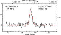
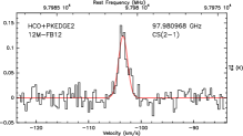
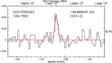
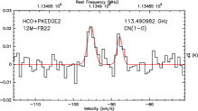
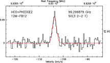
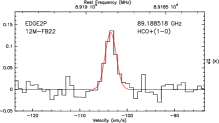
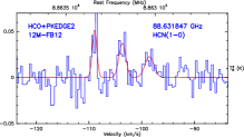
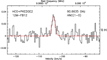
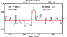
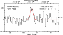
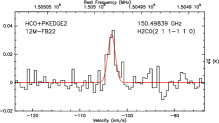
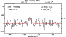
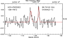
Figure 3: EC2 spectra observed at the ARO 12 m Feb-June 2002 position A ($\alpha_{2000}=$ 02:48:38.5,
$\delta=$ 58:28:28.1, $v_{\mathrm{rad}}=-103.70$ km s^-1). The ordinate is T${}_{R}^{*}$(K), uncorrected for beam-filling.

              

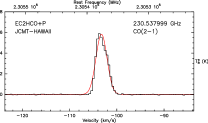
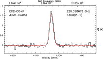
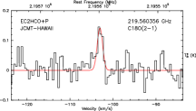
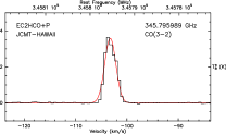
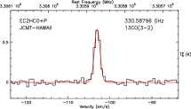
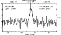
Figure 4: EC2 spectra observed at the JCMT 15 m June 2004 position A ($\alpha_{2000}=$ 02:48:38.5,
$\delta=$ 58:28:28.1, $v_{\mathrm{rad}}=-103.70$ km s^-1). The ordinate is T${}_{R}^{*}$(K), uncorrected for beam-filling.

       

Figure 6: IRAM 30 m Oct-Nov 2005 1.2 mm dust map centered on position EC2DUST1A ($\alpha_{2000}=$ 02:48:41.0, $\delta=$ 58:29:27.9) with CO 2–1 intensity contours from Fig. 5a superimposed. The rms noise for the map is 6.35 mJy/beam with a detected peak of 20.3 mJy/beam. Axis offsets in arcsec.

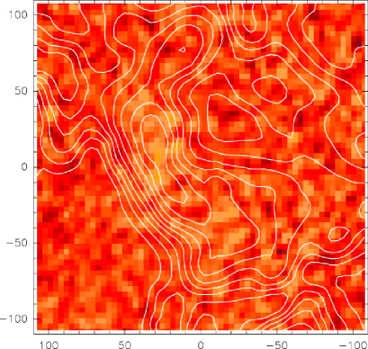
Figure 7: CO 2–1 intensity contours from EC2MAP1 (Fig. 5a) overlaid on 1.2 mm dust map (Fig. 6 EC2DUST1A), showing the correspondence of peak CO 2–1 and 1.2 mm dust emission. Axis offsets in arcsec.

                             

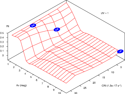
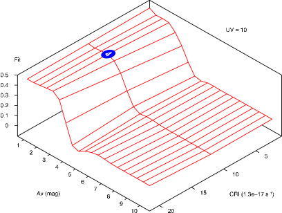
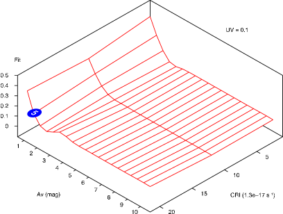
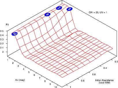
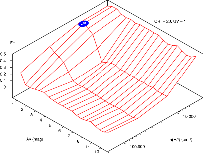
Figure 8: Agreement factor for models with varying: (a) $A_{\mathrm{V}}$ (mag) and cosmic ray ionisation (CRI); (b) $A_{\mathrm{V}}$ and CRI with UV field increased by a factor of 10 compared to local ISM values; (c) $A_{\mathrm{V}}$ and CRI with UV field reduced by a factor of 10; (d) $A_{\mathrm{V}}$ and an increasing UV field; (e) $A_{\mathrm{V}}$ and most initial abundances reducing relative to typical local ISM values; (f) $A_{\mathrm{V}}$ and $n(\mathrm{H}_{2})$. Unless indicated above, parameters were fixed at: $T$ = 20 K; $n(\mathrm{H}_{2})=1.2\times 10^{4}$ cm^-3; CRI rate = $20\times$ the standard ISM rate of $1.3\times 10^{-17}$ s^-1; UV field set to local ISM values; most initial abundances reduced by a factor of 5 from typical local ISM values (see Table 5). Numbered disks indicate specific models relative to the parameter surface.

        

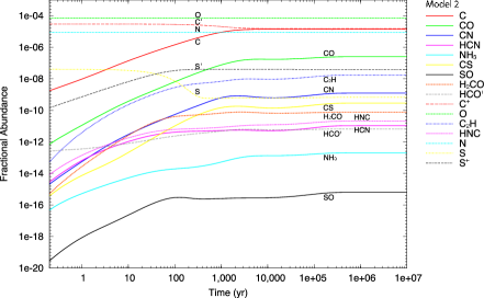
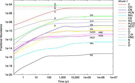
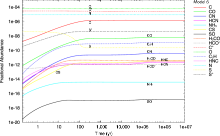
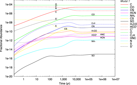
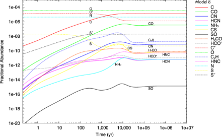
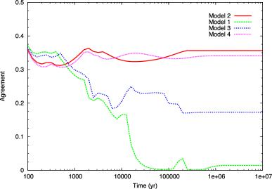
Figure 9: Fractional abundances varying over time (see Tables 7, 8 and 9) for:
(a) Model 2, where $A_{\mathrm{V}}$ = 1 mag, CRI = 20$\times$, UV = 1$\times$, IA = 0.2$\times$, $n$(H₂) = $1.2\times 10^{4}$ cm^-3, $T$ = 20 K;
(b) Model 4, where $A_{\mathrm{V}}$ = 2 mag, CRI = 10$\times$, UV = 10$\times$, IA = 0.2$\times$, $n$(H₂) = $1.2\times 10^{4}$ cm^-3, $T$ = 20 K;
(c) Model 6, where $A_{\mathrm{V}}$ = 1 mag, CRI = 20$\times$, UV = 20$\times$, IA = 0.2$\times$, $n$(H₂) = $1.2\times 10^{4}$ cm^-3, $T$ = 20 K;
(d) Model 7, where $A_{\mathrm{V}}$ = 3 mag, CRI = 20$\times$, UV = 40$\times$, IA = 0.2$\times$, $n$(H₂) = $1.2\times 10^{4}$ cm^-3, $T$ = 20 K;
(e) Model 8, where $A_{\mathrm{V}}$ = 2 mag, CRI = 20$\times$, UV = 1$\times$, IA = 0.1$\times$, $n$(H₂) = $1.2\times 10^{4}$ cm^-3, $T$ = 20 K.
(f) Agreement factor varying over time for Models 1–4, where $A_{\mathrm{V}}$ (mag) and cosmic ray ionisation (CRI) rates are varied (see Figs. 8a,b and Table 7).

References

- Bohlin et al. (1978) Bohlin, R. C., Savage, B. D., & Drake, J. F. 1978, ApJ, 224, 132
- Brand & Wouterloot (2007) Brand, J. & Wouterloot, J. G. A. 2007, A&A, 464, 909
- Braun & Burton (1999) Braun, R. & Burton, W. B. 1999, A&A, 341, 437
- Chiappini & Matteucci (1999) Chiappini, C. & Matteucci, F. 1999, Ap&SS, 265, 425
- Chiappini et al. (2001) Chiappini, C., Matteucci, F., & Romano, D. 2001, ApJ, 554, 1044
- Chiappini et al. (2003) Chiappini, C., Romano, D., & Matteucci, F. 2003, MNRAS, 339, 63
- Danby et al. (1988) Danby, G., Flower, D. R., Valiron, P., Schilke, P., & Walmsley, C. M. 1988, MNRAS, 235, 229
- de Geus et al. (1993) de Geus, E. J., Vogel, S. N., Digel, S. W., & Gruendl, R. A. 1993, ApJ, 413, L97
- Dickens et al. (2000) Dickens, J. E., Irvine, W. M., Snell, R. L., et al. 2000, ApJ, 542, 870
- Digel et al. (1994) Digel, S., de Geus, E., & Thaddeus, P. 1994, ApJ, 422, 92
- Digel et al. (1996a) Digel, S. W., de Geus, E. J., Henkel, C., Hüttemeister, S., & Thaddeus, P. 1996a, in IAU Symp. 170: CO: Twenty-Five Years of Millimeter-Wave Spectroscopy, 20P
- Digel et al. (1996b) Digel, S. W., Hunter, S. D., Mukherjee, R., et al. 1996b, in IAU Symp. 170: CO: 25 Years of mm-Wave Spectroscopy, 22
- Fich et al. (1989) Fich, M., Blitz, L., & Stark, A. A. 1989, ApJ, 342, 272
- Flower (1999) Flower, D. R. 1999, MNRAS, 305, 651
- Flower (2001) Flower, D. R. 2001, Journal of Physics B Atomic Molecular Physics, 34, 2731
- Frerking et al. (1982) Frerking, M. A., Langer, W. D., & Wilson, R. W. 1982, ApJ, 262, 590
- Green (1991) Green, S. 1991, ApJS, 76, 979
- Green (1994) Green, S. 1994, ApJ, 434, 188
- Henkel et al. (2000) Henkel, C., Mauersberger, R., Peck, A. B., Falcke, H., & Hagiwara, Y. 2000, A&A, 361, L45
- Henkel et al. (1980) Henkel, C., Walmsley, C. M., & Wilson, T. L. 1980, A&A, 82, 41
- Hildebrand (1983) Hildebrand, R. H. 1983, QJRAS, 24, 267
- Kobayashi & Tokunaga (2000) Kobayashi, N. & Tokunaga, A. T. 2000, ApJ, 532, 423
- Kobayashi et al. (2005) Kobayashi, N., Yasui, C., Tokunaga, A. T., & Saito, M. 2005, in Protostars and Planets V, 8639
- Kulkarni et al. (1982) Kulkarni, S. R., Heiles, C., & Blitz, L. 1982, ApJ, 259, L63
- Le Teuff et al. (2000) Le Teuff, Y. H., Millar, T. J., & Markwick, A. J. 2000, A&AS, 146, 157
- Levine et al. (2006) Levine, E. S., Blitz, L., & Heiles, C. 2006, Science, 312, 1773
- Lubowich et al. (2004) Lubowich, D. A., Brammer, G., Roberts, H., et al. 2004, in Origin and Evolution of the Elements
- Lubowich et al. (2000) Lubowich, D. A., Pasachoff, J. M., Balonek, T. J., et al. 2000, Nature, 405, 1025
- Maciel & Quireza (1999) Maciel, W. J. & Quireza, C. 1999, A&A, 345, 629
- MacLaren et al. (1988) MacLaren, I., Richardson, K. M., & Wolfendale, A. W. 1988, ApJ, 333, 821
- Mauersberger et al. (1990) Mauersberger, R., Henkel, C., & Sage, L. J. 1990, A&A, 236, 63
- Mauersberger et al. (1985) Mauersberger, R., Wilson, T. L., Walmsley, C. M., Henkel, C., & Batrla, W. 1985, A&A, 146, 168
- Pickett et al. (1998) Pickett, H. M., Poynter, R. L., Cohen, E. A., et al. 1998, J. Quant. Spectrosc. & Rad. Transfer, 60, 883
- Pratap et al. (1997) Pratap, P., Dickens, J. E., Snell, R. L., et al. 1997, ApJ, 486, 862
- Robin et al. (1992) Robin, A. C., Creze, M., & Mohan, V. 1992, ApJ, 400, L25
- Rogers et al. (2005) Rogers, A. E. E., Dudevoir, K. A., Carter, J. C., et al. 2005, ApJ, 630, L41
- Rolleston et al. (2000) Rolleston, W. R. J., Smartt, S. J., Dufton, P. L., & Ryans, R. S. I. 2000, A&A, 363, 537
- Ruffle (2006) Ruffle, P. M. E. 2006, PhD thesis, The University of Manchester, UK
- Ruffle et al. (2004) Ruffle, P. M. E., Zijlstra, A. A., Walsh, J. R., et al. 2004, MNRAS, 353, 796
- Schöier et al. (2005) Schöier, F. L., van der Tak, F. F. S., van Dishoeck, E. F., & Black, J. H. 2005, A&A, 432, 369
- Smartt et al. (1996) Smartt, S. J., Dufton, P. L., & Rolleston, W. R. J. 1996, A&A, 305, 164
- Snell et al. (2002) Snell, R. L., Carpenter, J. M., & Heyer, M. H. 2002, ApJ, 578, 229
- Stil & Irwin (2001) Stil, J. M. & Irwin, J. A. 2001, ApJ, 563, 816
- Takano et al. (1995) Takano, S., Nakai, N., & Kawaguchi, K. 1995, PASJ, 47, 801
- Tauber et al. (1995) Tauber, J. A., Lis, D. C., Keene, J., Schilke, P., & Buettgenbach, T. H. 1995, A&A, 297, 567
- Turner (2000) Turner, B. E. 2000, ApJ, 542, 837
- Turner et al. (1992) Turner, B. E., Chan, K.-W., Green, S., & Lubowich, D. A. 1992, ApJ, 399, 114
- Walmsley & Ungerechts (1983) Walmsley, C. M. & Ungerechts, H. 1983, A&A, 122, 164
- Watson et al. (1976) Watson, W. D., Anicich, V. G., & Huntress, W. T. 1976, ApJ, 205, L165
- Whittet (1992) Whittet, D. C. B. 1992, Dust in the galactic environment (The Graduate Series in Astronomy, Bristol: Institute of Physics Publishing)
- Wilson & Rood (1994) Wilson, T. L. & Rood, R. 1994, ARA&A, 32, 191
- Wouterloot & Brand (1996) Wouterloot, J. G. A. & Brand, J. 1996, A&AS, 119, 439
- Yasui et al. (2006) Yasui, C., Kobayashi, N., Tokunaga, A. T., Terada, H., & Saito, M. 2006, ApJ, 649, 753