Secure Communication over Fading Channels thanks: This research was supported by the National Science Foundation under Grant ANI-03-38807.

Yingbin Liang and H. Vincent Poor Department of Electrical Engineering
Princeton University
Princeton, NJ 08544, USA
Email: {yingbinl,poor}@princeton.edu
Abstract

The fading wire-tap channel is investigated, where the source-to-destination channel and the source-to-wire-tapper channel are corrupted by multiplicative fading gain coefficients in addition to additive Gaussian noise terms. The channel state information is assumed to be known at both the transmitter and the receiver. The parallel wire-tap channel with independent subchannels is first studied, which serves as an information-theoretic model for the fading wire-tap channel. Each subchannel is assumed to be a general broadcast channel and is not necessarily degraded. The secrecy capacity of the parallel wire-tap channel is established, which is the maximum rate at which the destination node can decode the source information with small probability of error and the wire-tapper does not obtain any information. This result is then specialized to give the secrecy capacity of the fading wire-tap channel, which is achieved with the source node dynamically changing the power allocation according to the channel state realization. An optimal source power allocation is obtained to achieve the secrecy capacity. This power allocation is different from the water-filling allocation that achieves the capacity of fading channels without the secrecy constraint.

I Introduction

Wireless communication has a broadcast nature, where security issues are captured by a basic wire-tap channel introduced by Wyner in [1]. In this model, a source node wishes to transmit confidential information to a destination node and wishes to keep a wire-tapper as ignorant of this information as possible. The performance measure of interest is the secrecy capacity, which is the largest reliable communication rate from the source node to the destination node with the wire-tapper obtaining no information. For the wire-tap channel where the channel from the source node to the destination and the wire-tapper is degraded, the secrecy capacity was given in [1] for the discrete memoryless channel and in [2] for the Gaussian channel. The general wire-tap channel without a degradedness assumption and with an additional common message for both the destination node and the wire-tapper was considered in [3], where the capacity-equivocation region and the secrecy capacity were given. The wire-tap channel was also considered recently for the fading and multiple antenna channels in [4, 5]. The secrecy capacity was addressed either for the case with a fixed fading state or from the outage probability viewpoint.

In this paper, we study the ergodic secrecy capacity of the fading wire-tap channel, which is the maximum secrecy rate that can be achieved over multiple fading states. We assume the fading gain coefficients of the source-to-destination channel and the source-to-wire-tapper channel are stationary and ergodic over time. We also assume both the transmitter and the receiver know the channel state information (CSI). Note that the CSI of the source-to-wire-tapper channel at the source can be justified as follows. In wireless networks, a node may be treated as a “wire-tapper” by a source node because it is not the intended destination of particular confidential messages. In this case, the “wire-tapper” is not a hostile node, and may also expect its own information from the same source node. Hence it is reasonable to assume that this “wire-tapper” feeds back the CSI to the source node.

The fading wire-tap channel can be viewed as a special case of the parallel wire-tap channel with independent subchannels in that the channel at each fading state realization corresponds to one subchannel. Hence we first study a parallel wire-tap channel with $L$ independent subchannels. Each subchannel is assumed to be a general broadcast channel and is not necessarily degraded, which is different from the model studied in [6]. This channel model also differs from the model studied in [6] in that the wire-tapper can receive outputs from all subchannels. The secrecy capacity of the parallel wire-tap channel is established. This result then specializes to the secrecy capacity of a parallel wire-tap channel with $K+M$ degraded subchannels, which is directly related to the fading wire-tap channel. For this model, we assume each of the $K$ subchannels satisfies the condition that the output at the wire-tapper is a degraded version of the output at the destination node, and each of the $M$ subchannels satisfies the condition that the output at the destination node is a degraded version of the output at the wire-tapper. We show that to achieve the secrecy capacity, it is optimal to keep the inputs to the $M$ subchannels null, i.e., use only the $K$ subchannels, and choose the inputs to the $K$ subchannels independently. Therefore, the secrecy capacity reduces to the sum of the secrecy capacities of the $K$ subchannels.

We further apply our result to obtain the secrecy capacity of the fading wire-tap channel. The fading wire-tap channel we study differs from the parallel Gaussian wire-tap channel studied in [7] in that we assume the source node is subject to an average power constraint over all fading state realization instead of each subchannel (channel corresponding to one fading state realization) being subject to a power constraint as assumed in [7]. Since the source node knows the CSI, it needs to optimize the power allocation among fading states to achieve the secrecy capacity. We obtain the optimal power allocation scheme, where the source node uses more power when the source-to-destination channel experiences a larger fading gain and the source-to-wire-tapper channel has a smaller fading gain. The secrecy capacity is not achieved by the water-filling allocation that achieves the capacity for the fading channel without the secrecy constraint.

In this paper, we use $X_{[1,L]}$ to indicate a group of variables $(X_{1},X_{2},\ldots,X_{L})$, and use $X_{[1,L]}^{n}$ to indicate a group of vectors $(X_{1}^{n},X_{2}^{n},\ldots,X_{L}^{n})$, where $X_{l}^{n}$ indicates the vector $(X_{l1},X_{l2},\ldots,X_{ln})$. Throughout the paper, the logarithmic function is to the base $2$.

The paper is organized as follows. We first introduce the parallel wire-tap channel with independent subchannels, and present the secrecy capacity for this channel. We next present the secrecy capacity for the fading wire-tap channel. We finally demonstrate our results by numerical examples.

II Parallel Wire-tap Channel

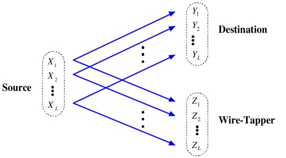
We consider a parallel wire-tap channel with $L$ independent subchannels (see Fig. 1), which consists of $L$ finite input alphabets $\mathcal{X}_{[1,L]}$, and $2L$ finite output alphabets $\mathcal{Y}_{[1,L]}$ and $\mathcal{Z}_{[1,L]}$. The transition probability distribution is given by

$$p(y_{[1,L]},z_{[1,L]}|x_{[1,L]})=\prod_{l=1}^{L}p_{l}(y_{l},z_{l}|x_{l})$$ (1)

where $x_{l}\in\mathcal{X}_{l}$, $y_{l}\in\mathcal{Y}_{l}$, and $z_{l}\in\mathcal{Z}_{l}$ for $l=1,\ldots,L$.

Note that each of the $L$ subchannels is assumed to be a general broadcast channel and is not necessarily degraded as assumed in [1]. Hence the model we study is more general than the parallel channel model studied in [6] which assumes each subchannel is less noisy [8].

Refer to caption
Figure 1: Parallel wire-tap channel

A $\left(2^{nR},n\right)$ code consists of the following:

  • $\bullet$

    One message set: $\mathcal{W}=\{1,2,\ldots,2^{nR}\}$ with the message $W$ uniformly distributed over $\mathcal{W}$;

  • $\bullet$

    One (stochastic) encoder at the source node that maps each message $w\in\mathcal{W}$ to a codeword $x_{[1,L]}^{n}$;

  • $\bullet$

    One decoder at the destination node that maps a received sequence $y_{[1,L]}^{n}$ to a message $w\in\mathcal{W}$.

The secrecy level of the message $W$ at the wire-tapper is measured by the equivocation rate defined as follows:

$$\frac{1}{n}H\left(W\Big{|}Z_{[1,L]}^{n}\right).$$ (2)

The higher the equivocation rate, the less information the wire-tapper obtains.

A rate-equivocation pair $(R,R_{e})$ is achievable if there exists a sequence of $\left(2^{nR},n\right)$ codes with the destination decoding error probability $P_{e}^{(n)}\rightarrow 0$ as $n$ goes to infinity and with the equivocation rate $R_{e}$ satisfying

$$R_{e}\leq\lim_{n\rightarrow\infty}\frac{1}{n}H\left(W\Big{|}Z_{[1,L]}^{n}\right).$$ (3)

We focus on the case where perfect secrecy is achieved, i.e., the wire-tapper does not obtain any information about the message $W$. This happens if $R_{e}=R$. The secrecy capacity $C_{s}$ is the maximum $R$ such that $(R,R_{e}=R)$ is achievable, i.e.,

$$C_{s}=\max_{\text{Achievable }(R,R_{e}=R)}R.$$ (4)

We obtain the following secrecy capacity result for the parallel wire-tap channel.

Theorem 1

The secrecy capacity of the parallel wire-tap channel with $L$ subchannels is

$$C_{s}=\sum_{l=1}^{L}C_{s}^{l}$$ (5)

where $C_{s}^{l}$ is the secrecy capacity of subchannel $l$ and is given by

$$C_{s}^{l}=\max\;I(U_{l};Y_{l})-I(U_{l};Z_{l})$$ (6)

where the maximum in the preceding equation is over the distributions $p(u_{l},x_{l})p(y_{l},z_{l}|x_{l})$, which satisfies the Markov chain condition $U_{l}\rightarrow X_{l}\rightarrow(Y_{l},Z_{l})$.

The proof of Theorem 1 is relegated to Section III.

In the following, we consider a parallel wire-tap channel, where each subchannel is either degraded such that the output at the wire-tapper is a degraded version of the output at the destination node, or degraded such that the output at the destination node is a degraded version of the output at the wire-tapper. This channel specializes to the fading wiretap channel that is considered in Section IV, and is hence of particular interest.

Refer to caption
Figure 2: Parallel wire-tap channel with $K+M$ degraded subchannels

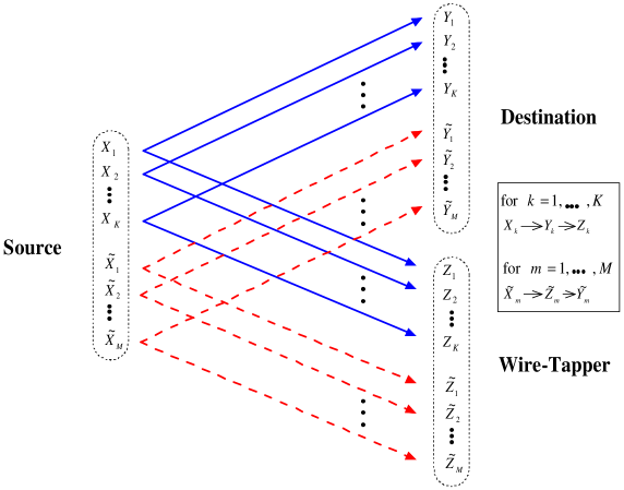
More formally, we define the channel described above to be the parallel wire-tap channel with $K+M$ degraded subchannels (see Fig. 2), which consists of $K+M$ finite input alphabets $\mathcal{X}_{[1,K]}$ and $\tilde{\mathcal{X}}_{[1,M]}$, $2(K+M)$ finite output alphabets $\mathcal{Y}_{[1,K]},\mathcal{Z}_{[1,K]},\tilde{\mathcal{Y}}_{[1,M]},$ and $\tilde{\mathcal{Z}}_{[1,M]}$. The transition probability distribution is given by

$$\begin{split}&p(y_{[1,K]},\tilde{y}_{[1,M]},z_{[1,K]},\tilde{z}_{[1,M]}|x_{[1,K]},\tilde{x}_{[1,M]})\\ &\hskip 14.22636pt=\prod_{k=1}^{K}p_{k}(y_{k},z_{k}|x_{k})\prod_{m=1}^{M}p_{m}(\tilde{y}_{m},\tilde{z}_{m}|\tilde{x}_{m})\end{split}$$ (7)

where $x_{k}\in\mathcal{X}_{k}$, $y_{k}\in\mathcal{Y}_{k}$, and $z_{k}\in\mathcal{Z}_{k}$ for $k=1,\ldots,K$, and $\tilde{x}_{m}\in\tilde{\mathcal{X}}_{m}$, $\tilde{y}_{m}\in\tilde{\mathcal{Y}}_{m}$, and $\tilde{z}_{m}\in\tilde{\mathcal{Z}}_{m}$ for $m=1,\ldots,M$. The probability distributions $p_{k}(y_{k},z_{k}|x_{k})$ and $p_{m}(\tilde{y}_{m},\tilde{z}_{m}|\tilde{x}_{m})$ satisfy the following degraded conditions:

$$\begin{split}&p_{k}(y_{k},z_{k}|x_{k})=p_{k}(y_{k}|x_{k})p_{k}(z_{k}|y_{k})\\ &\hskip 113.81102pt\text{for }k=1,\ldots,K,\\ &p_{m}(\tilde{y}_{m},\tilde{z}_{m}|\tilde{x}_{m})=p_{m}(\tilde{z}_{m}|\tilde{x}_{m})p_{m}(\tilde{y}_{m}|\tilde{z}_{m})\\ &\hskip 113.81102pt\text{for }m=1,\ldots,M;\end{split}$$ (8)

i.e., the following Markov chain conditions are satisfied

$$\begin{split}X_{k}\rightarrow&Y_{k}\rightarrow Z_{k}\hskip 34.14322pt\text{for }k=1,\ldots,K,\\ \tilde{X}_{m}\rightarrow&\tilde{Z}_{m}\rightarrow\tilde{Y}_{m}\hskip 28.45274pt\text{for }m=1,\ldots,M.\end{split}$$ (9)

The following secrecy capacity follows easily from Theorem 1.

Corollary 1

The secrecy capacity of the parallel wire-tap channel with $K+M$ degraded subchannels is

$$C_{s}=\sum_{k=1}^{K}C_{s}^{k}$$ (10)

where $C_{s}^{k}$ is the secrecy capacity of subchannel $k$ and is given by

$$C_{s}^{k}=\max_{p(x_{k})}\;I(X_{k};Y_{k})-I(X_{k};Z_{k}).$$ (11)
Remark 1

It is optimal to choose the inputs to the $K$ subchannels independently and set the inputs to the $M$ subchannels to be null. Hence the $M$ subchannels do not contribute to the secrecy capacity. This is intuitive because the wire-tapper obtains all information that the destination node obtains over the $M$ subchannels.

III Proof of Theorem 1

The achievability follows from [3, Corollary 2] by setting $U=(U_{1},\ldots,U_{L})$, $X=(X_{1},\ldots,X_{L})$, $Y=(Y_{1},\ldots,Y_{L})$, and $Z=(Z_{1},\ldots,Z_{L})$, and choosing the components of $U$ and $X$ to be independent.

To show the converse, we consider a code with length $n$ and average error probability $P_{e}$. The probability distribution on $W\times\mathcal{X}_{[1,L]}^{n}\times\mathcal{Y}_{[1,L]}^{n}\times\mathcal{Z}_{[1,L]}^{n}$ is given by

$$\begin{split}&p(w,x_{[1,L]}^{n},y_{[1,L]}^{n},z_{[1,L]}^{n})\\ &\hskip 14.22636pt=p(w)p(x_{[1,L]}^{n}|w)\prod_{i=1}^{n}\;\prod_{l=1}^{L}\;p_{l}(y_{li},z_{li}|x_{li})\end{split}$$ (12)

By Fano’s inequality [9, Sec. 2.11], we have

$$H(W|Y_{[1,L]}^{n})\leq nRP_{e}+1:=n\delta$$ (13)

where $\delta\rightarrow 0$ if $P_{e}\rightarrow 0$.

We now bound the equivocation rate $R_{e}$:

$$\begin{split}&nR_{e}\\ &\leq H\big{(}W|Z_{[1,L]}^{n}\big{)}\\ &=H\big{(}W|Z_{[1,L]}^{n}\big{)}-H(W)+H(W)\\ &\hskip 14.22636pt-H\big{(}W|Y_{[1,L]}^{n}\big{)}+H\big{(}W|Y_{[1,L]}^{n}\big{)}\\ &\overset{(a)}{\leq}I(W;Y_{[1,L]}^{n})-I(W;Z_{[1,L]}^{n})+n\delta\\ &=\sum_{l=1}^{L}\Big{[}I(W;Y_{l}^{n}|Y_{[1,l-1]}^{n})-I(W;Z_{l}^{n}|Z_{[l+1,L]}^{n})\Big{]}+n\delta\\ &=\sum_{l=1}^{L}\sum_{i=1}^{n}\Big{[}I(W;Y_{li}|Y_{[1,l-1]}^{n}Y_{l}^{i-1})\\ &\hskip 28.45274pt\hskip 14.22636pt-I(W;Z_{li}|Z_{l[i+1]}^{n}Z_{[l+1,L]}^{n})\Big{]}+n\delta\\ &\overset{(b)}{=}\sum_{l=1}^{L}\sum_{i=1}^{n}\Big{[}I(WZ_{l[i+1]}^{n}Z_{[l+1,L]}^{n};Y_{li}|Y_{[1,l-1]}^{n}Y_{l}^{i-1})\\ &\hskip 28.45274pt\hskip 14.22636pt-I(Z_{l[i+1]}^{n}Z_{[l+1,L]}^{n};Y_{li}|WY_{[1,l-1]}^{n}Y_{l}^{i-1})\\ &\hskip 28.45274pt\hskip 14.22636pt-I(WY_{[1,l-1]}^{n}Y_{l}^{i-1};Z_{li}|Z_{l[i+1]}^{n}Z_{[l+1,L]}^{n})\\ &\hskip 28.45274pt\hskip 14.22636pt+I(Y_{[1,l-1]}^{n}Y_{l}^{i-1};Z_{li}|WZ_{l[i+1]}^{n}Z_{[l+1,L]}^{n})\Big{]}+n\delta\\ &\overset{(c)}{=}\sum_{l=1}^{L}\sum_{i=1}^{n}\Big{[}I(WZ_{l[i+1]}^{n}Z_{[l+1,L]}^{n};Y_{li}|Y_{[1,l-1]}^{n}Y_{l}^{i-1})\\ &\hskip 28.45274pt\hskip 14.22636pt-I(WY_{[1,l-1]}^{n}Y_{l}^{i-1};Z_{li}|Z_{l[i+1]}^{n}Z_{[l+1,L]}^{n})\Big{]}+n\delta\\ &=\sum_{l=1}^{L}\sum_{i=1}^{n}\Big{[}I(Z_{l[i+1]}^{n}Z_{[l+1,L]}^{n};Y_{li}|Y_{[1,l-1]}^{n}Y_{l}^{i-1})\\ &\hskip 28.45274pt\hskip 14.22636pt+I(W;Y_{li}|Y_{[1,l-1]}^{n}Y_{l}^{i-1}Z_{l[i+1]}^{n}Z_{[l+1,L]}^{n})\\ &\hskip 28.45274pt\hskip 14.22636pt-I(Y_{[1,l-1]}^{n}Y_{l}^{i-1};Z_{li}|Z_{l[i+1]}^{n}Z_{[l+1,L]}^{n})\\ &\hskip 28.45274pt\hskip 14.22636pt-I(W;Z_{li}|Y_{[1,l-1]}^{n}Y_{l}^{i-1}Z_{l[i+1]}^{n}Z_{[l+1,L]}^{n})\Big{]}+n\delta\\ &\overset{(d)}{=}\sum_{l=1}^{L}\sum_{i=1}^{n}\big{[}I(W;Y_{li}|Y_{[1,l-1]}^{n}Y_{l}^{i-1}Z_{l[i+1]}^{n}Z_{[l+1,L]}^{n})\\ &\hskip 28.45274pt\hskip 14.22636pt-I(W;Z_{li}|Y_{[1,l-1]}^{n}Y_{l}^{i-1}Z_{l[i+1]}^{n}Z_{[l+1,L]}^{n})\Big{]}+n\delta\\ &\overset{(e)}{=}\sum_{l=1}^{L}\sum_{i=1}^{n}\Big{[}I(U_{li};Y_{li}|Q_{li})-I(U_{li};Z_{li}|Q_{li})\Big{]}+n\delta\\ \end{split}$$ (14)

where $(a)$ follows from Fano’s inequality, $(b)$ follows from the chain rule, $(c)$ and $(d)$ follow from Lemma 7 in [3], and $(e)$ follows from the following definition:

$$Q_{li}:=(Y_{[1,l-1]}^{n}Y_{l}^{i-1}Z_{l[i+1]}^{n}Z_{[l+1,L]}^{n}),\hskip 14.22636ptU_{li}=(WQ_{li}).$$ (15)

We note that $(Q_{li},U_{li},X_{li},Y_{li},Z_{li})$ satisfy the following Markov chain condition:

$$Q_{li}\rightarrow U_{li}\rightarrow X_{li}\rightarrow(Y_{li},Z_{li}).$$ (16)

We introduce a random variable $G$ that is independent of all other random variables, and is uniformly distributed over $\{1,2,\ldots,n\}$. Define $Q_{l}=(G,Q_{lG})$, $U_{l}=(G,U_{lG})$, $X_{l}=X_{lG}$, $Y_{l}=Y_{lG}$, and $Z_{l}=Z_{lG}$. Note that $(Q_{l},U_{l},X_{l},Y_{l},Z_{l})$ satisfy the following Markov chain condition:

$$Q_{l}\rightarrow U_{l}\rightarrow X_{l}\rightarrow(Y_{l},Z_{l}).$$ (17)

Using the above definitions, (14) becomes

$$R_{e}\leq\sum_{l=1}^{L}\Big{[}I(U_{l};Y_{l}|Q_{l})-I(U_{l};Z_{l}|Q_{l})\Big{]}+\delta$$ (18)

Therefore, an upper bound on $R_{e}$ is

$$R_{e}\leq\max\;\sum_{l=1}^{L}\Big{[}I(U_{l};Y_{l}|Q_{l})-I(U_{l};Z_{l}|Q_{l})\Big{]}+\delta$$ (19)

where the maximum is over the probability distributions $p(q_{[1,L]},u_{[1,L]},x_{[1,L]},y_{[1,L]},z_{[1,L]})$. Finally, we note that each term in the summation in (19) depends only on the distribution $p(q_{l},u_{l},x_{l},y_{l},z_{l})$. Hence there is no loss of optimality to consider only the distributions with the form $\prod_{l=1}^{L}p(q_{l},u_{l},x_{l})p(y_{l},z_{l}|x_{l})$. We also note that each term in the summation in (19) is maximized by a constant $Q_{l}$. Hence the following bound does not lose optimality:

$$R_{e}\leq\sum_{l=1}^{L}\max\Big{[}I(U_{l};Y_{l})-I(U_{l};Z_{l})\Big{]}+\delta$$ (20)

where the maximum for the $l$-th term in the summation is over the distributions $p(u_{l},x_{l})p(y_{l},z_{l}|x_{l})$ for $l=1,\ldots,L$. This concludes the converse proof.

IV Fading Wire-tap Channel

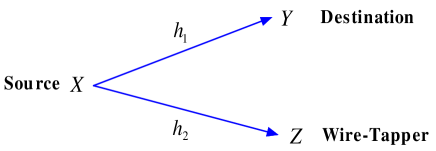
We study the fading wire-tap channel (see Fig. 3), where the source-to-destination channel and the source-to-wire-tapper channel are corrupted by multiplicative fading processes in addition to additive white Gaussian processes. The channel input-output relationship is given by

$$\begin{split}Y_{i}&=h_{1i}X_{i}+W_{i},\\ Z_{i}&=h_{2i}X_{i}+V_{i},\end{split}$$ (21)

where $i$ is the time index, and $X_{i}$ is the channel input at the time instant $i$, and $Y_{i}$ and $Z_{i}$ are channel outputs at the time instant $i$, respectively. The channel gain coefficients $h_{1i}$ and $h_{2i}$ are zero-mean proper complex random variables. We define $\underline{h}_{i}:=(h_{1i},h_{2i})$, and assume $\{\underline{h}_{i}\}$ is a stationary and ergodic vector random process. The noise processes $\{W_{i}\}$ and $\{V_{i}\}$ are zero-mean independent identically distributed (i.i.d.) proper complex Gaussian with $W_{i}$ and $V_{i}$ having variances $\mu^{2}$ and $\nu^{2}$, respectively. The input sequence $\{X_{i}\}$ is subject to the average power constraint $P$, i.e., $\frac{1}{n}\sum_{i=1}^{n}\mathrm{E}\big{[}X^{2}_{i}\big{]}\leq P$. We assume the channel state information (realization of $\underline{h}_{i}$) is known at both the transmitter and the receiver instantaneously. As we mentioned in the introduction, the source node gets the CSI of the channel to the wire-tapper when the wire-tapper is not an actual hostile node and is only not the intended destination node for a particular confidential message.

Refer to caption
Figure 3: Fading Wire-tap Channel

We first introduce the following lemma that follows from [10, lemma 1]. This lemma is useful to obtain the secrecy capacity of the fading wire-tap channel.

Lemma 1

The secrecy capacity of the wire-tap channel depends only on the marginal transition distributions $p(y|x)$ of the source-to-destination channel and $p(z|x)$ of the source-to-wire-tapper channel.

The following generalization of the result in [2] follows directly from Lemma 1.

Corollary 2

The secrecy capacity of the Gaussian wire-tap channel given in [2, Theorem 1] holds for the case with general correlation between the noise variables at the destination node and the wire-tapper.

Based on Lemma 1 and Corollary 1, we obtain the secrecy capacity of the fading wire-tap channel.

Theorem 2

The secrecy capacity of the fading wire-tap channel is

$$\begin{split}C_{s}=\max_{\mathrm{E}_{A}[P(\underline{h})]\leq P}\;\mathrm{E}_{A}\Bigg{[}&\log\left(1+\frac{P(\underline{h})|h_{1}|^{2}}{\mu^{2}}\right)\\ &-\log\left(1+\frac{P(\underline{h})|h_{2}|^{2}}{\nu^{2}}\right)\Bigg{]}.\end{split}$$ (22)

where $A:=\Big{\{}\underline{h}:\frac{|h_{1}|^{2}}{\mu^{2}}>\frac{|h_{2}|^{2}}{\nu^{2}}\Big{\}}$. The random vector $\underline{h}=(h_{1},h_{2})$ has the same distribution as the marginal distribution of the process $\{\underline{h}_{i}\}$ at one time instant.

The optimal power allocation that achieves the secrecy capacity in (22) is given by

$$P^{*}(\underline{h})=\begin{cases}\frac{1}{\lambda\ln 2}-\frac{\mu^{2}}{|h_{1}|^{2}},\hskip 14.22636pt\text{if }\;|h_{2}|^{2}=0,\;\;\lambda<\frac{1}{\ln 2}\frac{|h_{1}|^{2}}{\mu^{2}}\\ \\ \frac{1}{2}\sqrt{\left(\frac{\nu^{2}}{|h_{2}|^{2}}-\frac{\mu^{2}}{|h_{1}|^{2}}\right)\left(\frac{4}{\lambda\ln 2}-\frac{\mu^{2}}{|h_{1}|^{2}}+\frac{\nu^{2}}{|h_{2}|^{2}}\right)}\\ -\frac{1}{2}\left(\frac{\mu^{2}}{|h_{1}|^{2}}+\frac{\nu^{2}}{|h_{2}|^{2}}\right),\\ \\ \hskip 73.97733pt\text{if }\;|h_{2}|^{2}>0,\;\;\frac{|h_{1}|^{2}}{\mu^{2}}>\frac{|h_{2}|^{2}}{\nu^{2}},\\ \hskip 88.2037pt\lambda<\frac{1}{\ln 2}\left(\frac{|h_{1}|^{2}}{\mu^{2}}-\frac{|h_{2}|^{2}}{\nu^{2}}\right)\\ \\ 0,\hskip 62.59596pt\text{otherwise}\end{cases}$$ (23)

where $\lambda$ is chosen to satisfy the power constraint $\mathrm{E}_{A}[P(\underline{h})]=P$.

Remark 2

The optimal power allocation (23) to achieve the secrecy capacity is not water-filling. This is in contrast to the fading channel without the secrecy constraint where water-filling allocation is optimal to achieve the capacity [11].

Remark 3

The secrecy capacity in Theorem 2 is established for general fading processes $\{\underline{h}_{i}\}$ where only ergodic and stationary conditions are assumed. The fading process $\{\underline{h}_{i}\}$ can be correlated across time, and is not necessarily Gaussian. The two component processes $\{h_{1i}\}$ and $\{h_{2i}\}$ can be correlated as well.

Remark 4

The secrecy capacity in Theorem 2 is established for the case with general correlation between the noise variables $W_{i}$ and $V_{i}$.

Refer to caption
(a): $P^{*}(\underline{h})$ as a function of $(h_{1},h_{2})$
Refer to caption
(b): $P^{*}(\underline{h})$ as a function of $|h_{1}|^{2}$
Refer to caption
(c): $P^{*}(\underline{h})$ as a function of $|h_{2}|^{2}$
Figure 4: Optimal power allocation $P^{*}(\underline{h})$ for a Rayleigh fading wire-tap channel
Proof:

The fading wire-tap channel can be viewed as a parallel wire-tap channel with each subchannel having the following form

$$\begin{split}Y&=h_{1}X+W,\\ Z&=h_{2}X+V,\end{split}$$ (24)

where $(h_{1},h_{2})$ is a fixed channel realization of $\underline{h}$. Note that the subchannel (24) is not physically degraded. We now consider the following subchannel:

$\displaystyle Y=h_{1}X+W,\hskip 14.22636ptZ=\frac{h_{2}h_{1}^{*}}{|h_{1}|^{2}}(h_{1}X+W)+V^{\prime},$
 $\displaystyle\hskip 156.49014pt\text{ if }\;\underline{h}\in A$ (25)
$\displaystyle Y=\frac{h_{1}h_{2}^{*}}{|h_{2}|^{2}}(h_{2}X+V)+W^{\prime},\hskip 14.22636ptZ=h_{2}X+V,$
 $\displaystyle\hskip 159.3356pt\text{ if }\;\underline{h}\in A^{c}$ (26)

where $V^{\prime}$ and $W^{\prime}$ are zero mean proper complex Gaussian random variables with variances $\nu^{2}-\frac{|h_{2}|^{2}}{|h_{1}|^{2}}\mu^{2}$ and $\mu^{2}-\frac{|h_{1}|^{2}}{|h_{2}|^{2}}\nu^{2}$, respectively. The subchannel (25)/(26) is physically degraded, and has the same marginal distribution $p(y|x)$ and $p(z|x)$ as the subchannel (24). Hence by Lemma 1, the parallel wire-tap channel with subchannels having the form (24) and with subchannels having the form (25)/(26) have the same secrecy capacity. We can now apply Corollary 1 to the parallel wire-tap channel with subchannels having the form (25)/(26). Note that the subchannel (25) with $\underline{h}\in A$ is degraded in the same fashion as the $K$ subchannels in (8), and the subchannel (26) with $\underline{h}\in A^{c}$ is degraded in the same fashion as the $M$ subchannels in (8). From Corollary 1, it is clear that the subchannels with $\underline{h}\in A^{c}$ do not contribute to the secrecy capacity. The achievability of (22) now follows from (10) and (11) by setting the input distribution $X\sim\mathcal{CN}(0,P(\underline{h}))$ for $\underline{h}\in A$. Note that the summation $\sum_{k=1}^{K}$ in (10) becomes the average $\mathrm{E}_{\underline{h}\in A}$ for the fading channel.

The converse of (22) follows from the steps that are similar to those in [2].

We are now left to optimize (22) over power allocations satisfying $\mathrm{E}_{A}[P(\underline{h})]\leq P$. One can check that the following function of $P(\underline{h})$

$$\mathrm{E}_{A}\left[\log\left(1+\frac{P(\underline{h})|h_{1}|^{2}}{\mu^{2}}\right)-\log\left(1+\frac{P(\underline{h})|h_{2}|^{2}}{\nu^{2}}\right)\right]$$ (27)

is concave. The optimal $P^{*}(\underline{h})$ given in (23) can be derived by the standard Kuhn-Tucker condition (see e.g., [12, p. 314-315]). ∎

V Numerical Results

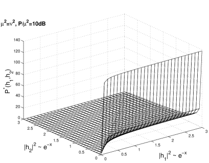
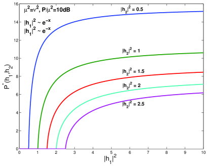
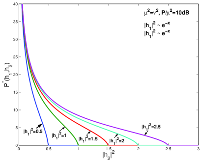
We first consider the Rayleigh fading wire-tap channel, where $h_{1}$ and $h_{2}$ are zero mean proper complex Gaussian random variables with variances 1. Hence $|h_{1}|^{2}$ and $|h_{2}|^{2}$ are exponentially distributed with parameter $1$. In Fig. 4 (a), we plot the optimal power allocation $P^{*}(\underline{h})$ as a function of $\underline{h}$. It can be seen from the graph that most of the source power is allocated to the channel states with small $|h_{2}|^{2}$. This behavior is shown more clearly in Fig. 4 (b), which plots $P^{*}(\underline{h})$ as a function of $|h_{1}|^{2}$ for different values of $|h_{2}|^{2}$, and in Fig. 4 (c), which plots $P^{*}(\underline{h})$ as a function of $|h_{2}|^{2}$ for different values of $|h_{1}|^{2}$. The source node allocates more power to the channel states with larger $|h_{1}|^{2}$ to forward more information to the destination node, and allocates less power for the channel states with larger $|h_{2}|^{2}$ to prevent the wire-tapper to obtain information. It can also be seen from Fig. 4 (b) and Fig. 4 (c) that the source node transmits only when the source-to-destination channel is better than the source-to-wire-tapper channel.

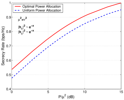
Fig. 5 plots the secrecy capacity achieved by the optimal power allocation, and compares it with the secrecy rate achieved by a uniform power allocation, i.e., allocating the same power for all channel states $\underline{h}\in A$. It can be seen that the uniform power allocation does not provide performance close to the secrecy capacity for the SNRs of interest. This is in contrast to the Rayleigh fading channel without the secrecy constraint, where the uniform power allocation can be close to optimum even for moderate SNRs. This also demonstrates that the exact channel state information is important to achieve higher secrecy rate.

Refer to caption
Figure 5: Comparison of secrecy capacity by optimal power allocation with secrecy rate by uniform power allocation for a Rayleigh fading wire-tap channel

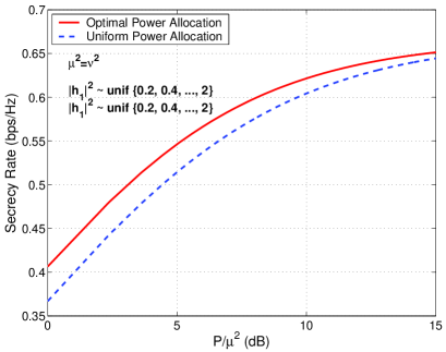
We next consider a fading wire-tap channel, where $|h_{1}|^{2}$ and $|h_{2}|^{2}$ are uniformly distributed over finite mass points $\{0.2,0.4,\ldots,2\}$. It can be seen from Fig. 6 that the secrecy rate achieved by the uniform power allocation approaches the secrecy capacity as SNR increases. Hence the uniform power allocation can be close to optimum for certain distributions of the fading gain coefficients.

Refer to caption
Figure 6: Comparison of secrecy capacity by optimal power allocation with secrecy rate by uniform power allocation for a uniformly distributed fading wire-tap channel

VI Conclusions

We have established the secrecy capacity for the parallel wire-tap channel with independent subchannels. We have further applied this result to obtain the secrecy capacity for the fading wire-tap channel, where the channel state information is assumed to be known at both the transmitter and the receiver. In particular, we have derived the optimal power allocation scheme to achieve the secrecy capacity. Our numerical results demonstrate that the channel state information at the transmitter is useful to improve the secrecy capacity.

References

  • [1] A. D. Wyner, “The wire-tap channel,” Bell Syst. Tech. J., vol. 54, no. 8, pp. 1355–1387, Oct. 1975.
  • [2] S. K. Leung-Yan-Cheong and M. E. Hellman, “The Gaussian wire-tap channel,” IEEE Trans. Inform. Theory, vol. 24, no. 4, pp. 451–456, July 1978.
  • [3] I. Csisz$\acute{\text{a}}$r and J. K$\ddot{\text{o}}$rner, “Broadcast channels with confidential messages,” IEEE Trans. Inform. Theory, vol. 24, no. 3, pp. 339–348, May 1978.
  • [4] P. Parada and R. Blahut, “Secrecy capacity of SIMO and slow fading channels,” in Proc. IEEE Int. Symp. Information Theory (ISIT), Adelaide, Australia, Sept. 2005, pp. 2152–2155.
  • [5] J. Barros and M. R. D. Rodrigues, “Secrecy capacity of wireless channels,” in Proc. IEEE Int. Symp. Information Theory (ISIT), Seattle, WA, USA, July 2006.
  • [6] H. Yamamoto, “Coding theorem for secret sharing communication systems with two noisy channels,” IEEE Trans. Inform. Theory, vol. 35, no. 3, pp. 572–578, May 1989.
  • [7] ——, “A coding theorem for secret sharing communication systems with two Gaussian wiretap channels,” IEEE Trans. Inform. Theory, vol. 37, no. 3, pp. 634–638, May 1991.
  • [8] J. K$\ddot{\text{o}}$rner and K. Marton, “Comparison of two noisy channels,” in Topics in Information Theory.   Keszthely (Hungary): Colloquia Math. Soc. J$\acute{a}$nos Bolyai, Amsterdam: North-Holland Publ., 1977, 1975, pp. 411–423.
  • [9] T. M. Cover and J. A. Thomas, Elements of Information Theory.   New York: Wiley, 1991.
  • [10] Y. Liang and H. V. Poor, “Generalized multiple access channels with confidential messages,” in Proc. IEEE Int. Symp. Information Theory (ISIT), Seattle, WA, USA, July 2006.
  • [11] A. Goldsmith and P. Varaiya, “Capacity of fading channels with channel side information,” IEEE Trans. Inform. Theory, vol. 43, no. 6, pp. 1986–1992, Nov. 1997.
  • [12] D. G. Luenberger, Linear and Nonlinear Programming, Second Edition.   Kluwer Academic Publishers, 2003.