Low angular momentum accretion in the collapsar: how long can be a long GRB?

Abstract

The collapsar model is the most promising scenario to explain the huge release of energy associated with long duration gamma-ray-bursts (GRBs). Within this scenario GRBs are believed to be powered by accretion through a rotationally support torus or by fast rotation of a compact object. In both cases then, rotation of the progenitor star is one of the key properties because it must be high enough for the torus to form, the compact object to rotate very fast, or both. Here, we check what rotational properties a progenitor star must have in order to sustain torus accretion over relatively long activity periods as observed in most GRBs. We show that simple, often cited, estimates of the total mass available for torus formation and consequently the duration of a GRB are only upper limits. We revise these estimates by taking into account the long term effect that as the compact object accretes the minimum specific angular momentum needed for torus formation increases. This in turn leads to a smaller fraction of the stellar envelope that can form a torus. We demostrate that this effect can lead to a significant, an order of magnidute, reduction of the total energy and overall duration of a GRB event. This of course can be mitigated by assuming that the progenitor star rotates faster then we assumed. However, our assumed rotation is already high compared to observational and theoretical constraints. We estimate the GRB duration times, first by assuming a constant accretion rate, as well as by explicitly calculating the free fall time of the gas during the collapse. We discuss the implications of our results.

1 Introduction

The collapsar model for a gamma ray burst invokes a presence of an accretion torus around a newly born black hole (Woosley 1995; Paczyński 1998; MacFadyen & Woosley 1999). The accretion energy is being transferred to the jet that propagates through the collapsar envelope and at some distance from the central engine is responsible for producing gamma rays. This type of model is commonly accepted as a mechanism for a long gamma ray burst production, because the whole event can last as long as the fallback material from the collapsar envelope is available to fuel the accretion disk or torus.

However, one should bear in mind that the rotating torus may form only when the substantial amount of specific angular momentum is carried in the material (see e.g. Lee & Ramirez-Ruiz 2006 for a recent study of this problem). This can be parameterized by the so called critical specific angular momentum value, which is dependent on the mass of the black hole, i.e. $l_{\rm crit}=2R_{\rm g}c$, where $R_{\rm g}$ is the gravitational radius. Because the black hole mass is not constant during the collapsar evolution, but increases as the envelope material accretes onto it, the critical angular momentum will change in time. Consequently, the amount of the rotating material, which was initially available for the torus formation, may become insufficient at a later stage of the collapsar evolution.

Moreover, the spin of the black hole will be changed by accretion. Whether the black hole can achieve a spin parameter close to the maximum one, depends on the properties of the accreted mass. While a large spin ($a\sim 0.9$) is thought to be a necessary condition for the jet launching (Blandford & Znajek 1977), it may happen that not enough specific angular momentum is being transferred to the black hole as its mass increases.

Another challenge for the collapsar model is due to the effects of stellar wind, which removes from the Wolf-Rayet stars a large fraction of angular momentum (Langer 1998). However, the winds of massive stars are relatively weaker in the low metallicity environment (Abbott et al. 1982), and possibly the GRB progenitor stars can rotate faster than an average W-R star (Vink 2007).

Here we address the question of whether the collapsing star envelope contains enough specific angular momentum in order to support the formation of the torus. Furthermore, it will be interesting to study the problem of spin up and spin down of the newly born black hole, and we shall consider this in a follow up paper. These two are the key properties needed to launch the GRB jet for an extended period of time. Because the angular momentum distribution in the Wolf-Rayet stars is unknown, we may pose this question also in a different way: we want to check how much angular momentum has to be initially present in the stellar envelope in order to allow for a long GRB production.

In Section 2, we describe the model of the initail conditions and evolution of the collapsing star, adopting various prescriptions for the angular momentum distribution and different scenarios of the accretion process. In Section 3, we present the results for the mass accreted onto the black hole in total and through the torus. We also estimate the resulting GRB durations, first in case of a constant $\dot{m}$ and then by explicitly calculating the free fall velocity of the gas accreting in the torus. Finally in Section 4, we discuss the resulting duration time of GRBs, as a function of the distribution of the specific angular momentum in the progenitor star.

2 Model

In the initial conditions, we use the spherically symmetric model of the 25 $M_{\odot}$ pre-supernova (Woosley & Weaver 1995). The same model was used by Proga et al. (2003) in their MHD simulation of the collapsar. Figure 1 shows the density profile and the mass enclosed inside a given radius. The Figure also shows the free fall timescale onto the enclosed mass, corresponding to the radius.

Figure 1: The density and mass profiles in the pre-supernova model. The data are taken from Woosley & Weaver (1995), model No. S251S7B@14233. The x-axis on the upper panel shows the free fall timescale corresponding to the radius shown on the lower panel’s x-axis.

The angular momentum within a star or rotating torus may depend on radius (see e.g. Woosley 1995, Jaroszyński 1996, Daigne & Mochkovitch 1997 for various prescriptions). Here we parameterize this distribution to be either a function of the polar angle $\theta$ (simplest case; models A and B), or a function of both radius $r$ and $\theta$ (models C and D).

First, we assume the specific angular momentum to depend only on the polar angle:

$$l_{\rm spec}=l_{0}f(\theta).$$ (1)

We constitute two different functions:

$$f(\theta)=1-|\cos\theta|~{}~{}{\rm(model~{}{\bf A})}$$ (2)

$$f(\theta)=\sin^{2}\theta~{}~{}{\rm(model~{}{\bf B})}$$ (3)

The rotation velocity is therefore given by:

$$v_{\varphi}={l_{0}\over r\sin\theta}f(\theta)$$ (4)

The normalization of this dependence is defined with respect to the critical specific angular momentum for the seed black hole:

$$l_{0}=xl_{\rm crit}(M^{0}_{\rm BH})=x\times 3.54\times 10^{16}{M[M_{\odot}]\over 2}~{}~{}{\rm cm^{2}~{}s^{-1}}$$ (5)

where $R_{\rm g}=2GM^{0}_{\rm BH}/c^{2}$ is the Schwarzschild radius (non-rotating black hole).

Second, we assume that the specific angular momentum will depend on the polar angle, as well as on the radius in the envelope, as:

$$l_{\rm spec}=l_{0}g(r)f(\theta),$$ (6)

We adopt the following functions:

$$l_{\rm spec}=xl_{\rm crit}({r\over r_{\rm core}})^{2}\sin^{2}\theta~{}~{}{\rm(model~{}{\bf C})}$$ (7)

$$l_{\rm spec}=x\sqrt{8GM_{\rm core}r}\sin^{2}\theta~{}~{}{\rm(model~{}{\bf D})}$$ (8)

The above model C corresponds to the rotation with a constant angular velocity $\Omega$, while the model D corresponds to a constant ratio between the centrifugal and gravitational forces. Note that the strong increase of $l_{\rm spec}$ with radius will lead to a very fast rotation at large radii. Therefore, a cut off may be required at some maximum value, $l_{\rm max}$ (see below).

The normalization of all the models is chosen such that the specific angular momentum is always equal to the critical value at $\theta=90^{\circ}$, and at $r=r_{\rm core}$ if the model depends on radius. In Section 3, we present the results of our calculations considering a range of initial values of $x$.

Initially, the mass of the black hole is given by the mass of the iron core of the star:

$$M_{BH}^{0}=M_{\rm core}=4\pi\int_{0}^{r_{\rm core}}\rho r^{2}dr.$$ (9)

For a given $x$, a certain fraction mass of the collapsar envelope, $M^{0}_{1}$, carries a specific angular momentum smaller than critical $l_{\rm crit}^{0}\equiv l_{\rm crit}(M_{\rm BH}^{0})$:

$$M^{0}_{1}=2\pi\int_{r_{\rm core}}^{r_{\rm max}}\int_{0}^{\pi}\rho_{1}r^{2}\sin\theta d\theta dr$$ (10)

where $\rho_{1}\equiv\rho(r,\theta)|_{l<l^{0}_{\rm crit}}$ is the density in the envelope where the specific angular momentum is smaller than critical. Here, the radius $r_{\rm max}$ is the size of the star. Correspondingly, by $M^{0}_{2}$ we denote the fraction of the envelope mass that carries the specific angular momentum larger or equal to the critical, with $\rho_{2}\equiv\rho(r,\theta)|_{l\geq l^{0}_{\rm crit}}$, and the total envelope mass is $M^{0}_{\rm env}=M^{0}_{1}+M^{0}_{2}$. Only the mass $M^{0}_{2}$ can form the torus around the black hole of the mass $M^{0}_{\rm BH}$.

The above relations set up the initial conditions for the torus formation in the collapsar, and $l_{\rm crit}$ is defined by the mass of the iron core, $M_{\rm core}$. However, as the collapse proceeds, the mass of the black hole will increase and the critical specific angular momentum will be a function of the increasing mass: $l_{\rm crit}(M_{\rm BH})$. The main point of this work is to compute the mass of the progenitor with $l>l_{\rm crit}$, taking into account this effect. Below, we redefine $\rho_{1}$ and $\rho_{2}$, so that the $l_{\rm crit}-M_{\rm BH}$ relation is taken into account.

To compute the mass of the envelope part that has high enough $l$ to form a torus around a given BH, and to estimate the time duration of the GRB powered by accretion, we need to know the mass of this black hole. A current $M_{\rm BH}$ depends on the mass of the mass of the seed black hole and the accretion scenario. We approximate this scenario in a following way. We assume that accretion is nonhomologous and BH grows by accreting mass $\Delta m^{\rm k}$, which is a function of the mass of a shell between the radius $r_{\rm k}$ and $r_{\rm k}+\Delta r_{\rm k}$ (see e.g. Lin & Pringle 1990). Formally, we perform the calculations of $M_{\rm BH}$ and $\Delta m^{\rm k}$ iteratively:

$$M_{\rm BH}^{\rm k}=M_{\rm BH}^{\rm k-1}+\Delta m^{\rm k}$$ (11)

where the increment of mass of the black hole is :

$$\Delta m^{\rm k}=2\pi\int_{r_{\rm k}}^{r_{\rm k}+\Delta r_{\rm k}}\int_{0}^{\pi}\bar{\rho}r^{2}\sin\theta d\theta dr$$ (12)

Here $\bar{\rho}$ depends on the accretion scenario (see below) and contains the information of the specific angular momentum distribution. The above two equations define an iterative procedure due to the nonlinear dependence of $\bar{\rho}$ on $M_{\rm BH}$. We start from the radius $r_{0}=r_{\rm core}$, i.e. that of an iron core.

We distinguish here three possible accretion scenarios:
(a) the accretion onto black hole proceeds at the same rate both from the torus and from the gas close to the poles, with $l<l^{\rm k}_{\rm crit}$, i.e. $\bar{\rho}\equiv\rho$ (and does not depend on $\theta$);
(b) the envelope material with $l<l^{\rm k}_{\rm crit}$ falls on the black hole first. Thus, until the polar funnel is evacuated completely, only this gas contributes to the black hole mass, i.e. $\bar{\rho}\equiv\rho_{1}$. After that, the material with $l>l^{\rm k}_{\rm crit}$ accretes, and $\bar{\rho}\equiv\rho_{2}$;
(c) the accretion proceeds only through the torus, and only this material contributes to the black hole growth i.e. $\bar{\rho}\equiv\rho_{2}$. In this case the rest of the envelope material is kept aside until the torus is accreted.

The densities $\rho_{1}$ and $\rho_{2}$, defined above, depend on $l_{\rm crit}^{\rm k}\equiv l_{\rm crit}(M^{\rm k}_{\rm BH})$. The above accretion scenarios are illustrated in the Figure 2. The panel (a) shows the scenario of a uniform accretion, in which the whole envelope material falls into black hole, regardless of its specific angular momentum. The red color marks the material with $l<l^{\rm k}_{\rm crit}$. The blue colors mark the material with $l>l^{\rm k}_{\rm crit}$, and when the black hole is small, this condition is satisfied for a larger range of $\theta$ (dark blue). When the black hole increases, the material with $l>l^{\rm k}_{\rm crit}$ occupies narrower $\theta$ range (light blue). The panel (b) shows the scenario with two steps: first the material with $l<l^{\rm k}_{\rm crit}$ accretes onto the black hole, increasing its mass; after this material is exhausted, the material with $l>l^{\rm k}_{\rm crit}$ starts accreting. Because the black hole mass has already increased, material with large $l$ is concentrated very close to the equator. The panel (c) shows the scenario in which only the material with $l>l^{\rm k}_{\rm crit}$ accretes.

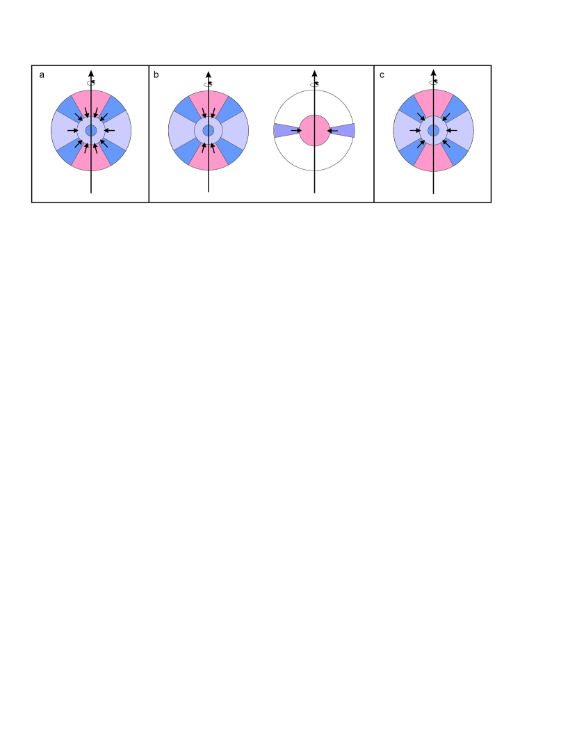
Figure 2: The scheme of accretion scenarios. The red color indicates the material with $l<l_{\rm crit}$. The blue colors indicate the material with $l>l_{\rm crit}$: darker for smaller black hole mass, and lighter for larger black hole mass. Arrows indicate, which material is accreting and contributes to the black hole growth.

In scenario a the mass accretion rate does not depend on the specific angular momentum. This is a very special and simple scenario. In reality, the accretion rate can depend on the specific angular momentum. For example, if an accreting torus produces a very powerful outflow, the weakly rotating polar material could be expelled and never reach the black hole (scenario c). This would also be a special and extreme situation. It is more likely that both the polar and disk material accrete but at different rates. However, it is unclear what these rates are and detailed simulations of MHD flows show that the rates can depend on time. For example, there are periods of time when the polar material accretes faster than the disk material and vice versa (e.g. Proga & Begelman 2003). To bracket this more realistic situation, we consider here another extreme and rather artificial scenario b, which corresponds to an somewhat ’reversed’ scenario c. In this scenario, initially the torus accretion rate is zero and accretion is dominated by the polar material. Only after the polar mateial is exhausted, the torus accretion starts. We note that although this scenario is quite extreme, it may be relevant if jets in GRBs must be very clean and light because in this scenario jets will be moving in the ’empty’ polar funnels.

Due to the increasing mass of the black hole, the critical angular momentum also increases, and as a result less and less material can satisfy the condition for the torus formation ($l>l^{\rm k}_{\rm crit}$). We stop the calculations, when there is no material with $l>l^{\rm k}_{\rm crit}$, i.e. able to form the torus:

$$w_{\rm k}={M_{2}^{\rm k}\over M_{\rm env}^{\rm k}}={2\pi\int^{r_{\rm max}}_{r_{\rm k+\Delta r}}\int_{0}^{\pi}\rho_{2}r^{2}\sin\theta d\theta dr\over 4\pi\int^{r_{\rm max}}_{r_{\rm k+\Delta r}}\rho r^{2}dr}=0.$$ (13)

Alternatively, the iterations may be stopped earlier, for example if we impose a physical limit based on the free fall timescale or the accretion rate, to be adequate to power the prompt GRB phase.

The duration of the GRB could be estimated as the ratio between the mass accreted through the torus, and the accretion rate $\dot{m}$:

$$M^{\rm torus}_{\rm accr}=\sum_{\rm k=1}^{k_{\rm max}}M_{2}^{\rm k}$$ (14)

$$\Delta t_{\rm GRB}={M_{\rm accr}^{\rm torus}\over\dot{m}}$$ (15)

where the number $k_{\rm max}$ is defined by the Equation 13.

Note that we assume here the GRB prompt emission is equal to the duration of the torus replenishment. In principle, $\dot{m}$ may depend on time. Here we take two approaches. First, for simplicity, we assume a constant accretion rate of a moderate value ($\dot{m}=0.01-1.0$ M_⊙ s^-1, see e.g. Popham, Woosley & Fryer 1999; Janiuk et al. 2004). Second, in more detailed calculations we determine the instantaneous accretion rate during the iterations, determined by the free fall velocity of gas in the torus.

3 Results

3.1 Models with the specific angular momentum dependent only on $\theta$

The Figure 3 shows the initial fraction of the envelope mass which contains large enough angular momentum to form the rotating torus, $w_{0}\equiv M^{0}_{2}/M^{0}_{\rm env}$ (see Eq. 13) for models A and B. For instance, for the adopted function $f(\theta)$ given by Eq. 2 (model A), and for the initial angular momentum normalization of $x=1.15$, we obtain $w_{0}=0.13$. This means that only 13% of the total mass of the envelope will initially be able to form the torus, while the remaining 87% of the envelope mass will fall radially towards black hole. On the other hand, for $x>5$, more than 75% of the envelope mass will be rotating fast enough to contribute to the torus formation. The model B gives systematically larger values of $w_{0}$ and for $x=1.15$, we have $w_{0}=0.36$, while for $x>5$ we have more than 85% of the envelope mass able to form the torus.

Figure 3: The initial mass fraction of material with the angular momentum $l>l_{\rm crit}$, as a function of the initial normalization of the specific angular momentum distribution, for model A (solid squares) and model B (open circles) of the distribution function $f(\theta)$.

As we show below, these are only the upper limits for the mass that could be accreted through the torus, and drive the GRB duration. These values will be much smaller, when we calculate the collapsar evolution with increasing $l^{\rm k}_{\rm crit}$ instead of $l^{\rm 0}_{\rm crit}$.

The Figure 4 shows $l^{\rm k}_{\rm crit}$, i.e. $l_{\rm crit}$ as a function of the current radius $r_{\rm k}$, which is the inner radius of the collapsing envelope in a subsequent step $k$. The figure thus shows how the critical specific angular momentum changes with time during the collapse, for an exemplary value of $x=7$.

The $l_{\rm crit}$ rises with time, as the black hole accretes mass from the envelope, and corresponds to a changing black hole mass. The most steep rise is for the uniform accretion scenario a, and in this case by definition the result does not depend on the adopted distribution function for the specific angular momentum, $f(\theta)$. Therefore both curves marked by a solid line overlap. Also, in scenario a the plotted curves do not depend on $x$, as well as neither on the slope nor on the location of the curve. The latter influences only the maximum of this curve, as for larger $x$ we have more material available to form the torus. In particular, for $x=7$, the two overlapping curves shown in the figure end at $r\sim 10^{13}$ cm.

For the scenario c, i.e. accretion of gas with $l>l^{\rm k}_{\rm crit}$, $l_{\rm crit}$ rises less steeply with $r_{\rm k}$ than in scenario a, because now less material is contributing to the black hole mass. In this case $f(\theta)$ affects the results, and model A gives systematically smaller values of $l_{\rm crit}$ than model B.

For the scenario b, the result is very sensitive to $x$, and we can have either one or two phases of accretion: only the polar inflow or first the polar inflow and then torus accretion. The value of $x=7$ was chosen, because in model A still no torus is able to form, and we have only phase 1, while in model B this value of $x$ is already large enough and the phase 2 occurs.

For phase 1 in scenario b (marked by the thinner lines in the figure), i.e. the material with $l<l^{\rm k}_{\rm crit}$ is accreting, the dependence on $f(\theta)$ is the following: model A adds more mass to the black hole and therefore it leads to the larger values of $l_{\rm crit}$ than model B. For phase 2 of scenario b (present only for model B and marked by the thick line in the figure), the evolution starts from the last $l^{\rm k}_{\rm crit}$ achieved in the end of phase 1. Then $l^{\rm k}_{\rm crit}$ increases, and ultimately reaches the final solution of models Bc and Ab, because this $l_{\rm crit}$ corresponds to the black hole mass that has increased maximally: either only through a torus, or first through the through the polar funnels and then through the torus accretion.

All the curves in Figure 4 exhibit a characteristic evolution of their slopes, tracing the density distribution in the progenitor star (see the top panel of Figure 1). First, the fast rise is due to accretion of the most dense inner shells of the stellar envelope. Then, the slope flattens, as the density in the envelope decreases and the mass does not grow very fast. In the end, the slope of $l^{\rm k}_{\rm crit}\equiv l_{\rm crit}(r_{\rm k})\equiv l_{\rm crit}(M_{\rm BH})$ rises again, due to larger volume of the shells, but this rise is depending on the adopted scenario. In scenario c the sequence is the following: increase of $l^{\rm k}_{\rm crit}$ $\rightarrow$ more accretion $\rightarrow$ larger increase of $l^{\rm k}_{\rm crit}$ $\rightarrow$ less accretion. In the phase 1 of scenario b, such an equilibrium is not established, because the accretion onto black hole proceeds through the polar funnels, i.e. using the material with $l<l^{\rm k}_{\rm crit}$, so we have: increase of $l^{\rm k}_{\rm crit}$ $\rightarrow$ more accretion $\rightarrow$ further increase of $l^{\rm k}_{\rm crit}$, and for large radii $r_{\rm k}$ the slope of the curves shown in Fig. 4 in this scenario is much steeper. The phase 2 of scenario b results in the changes of the slope of $l^{\rm k}_{\rm crit}$ similar to other scenarios, a and b (provided that the phase 2. occurs).

Figure 4: The critical specific angular momentum as a function of radius within which the envelope mass collapsed onto BH. The results are shown for one exemplary value of the initial normalization parameter, $x=l_{0}/l_{crit}=7$. The models of the distribution function $f(\theta)$ are: A (solid squares) and B (open circles), and accretion scenarios are: a (solid line), b (short dashed line) and c (long dashed line). The thin line for model Bb represents the results from the phase 1 of accretion (through the poles), while the thicker line Bb represents the results from the phase 2 (torus accretion). Note, that for the model Ab there is only a thin line, and no phase 2, because for $x=7$ the torus does not form. Note also, that the solid lines (i.e. models Aa and Ba overlap.

In Figure 5, we show the total mass accreted onto a black hole, and in Figure 6 we show the mass accreted through the torus, both as a function of $x$. Figure 6 can be also regarded as showing the estimated duration of a GRB, if the accretion rate is constant. The results are again presented for the 3 scenarios of accretion: a, b and c (marked by solid, short-dashed and long dashed lines, respectively), as well as for the two prescriptions for the function $f(\theta)$, models A and B (marked by squares and circles, respectively). The upper panels in Figs. 5 and 6 show the results obtained is case of the maximum limit for the free fall time set yo $t_{\rm ff}^{\rm max}=1000$ s.

The values of the total accreted mass are the largest for the scenario of the uniform accretion, a. Depending on $x$, the black hole mass is growing until there is no further material with $l>l^{\rm k}_{\rm crit}$.

Figure 5: The total mass accreted onto a black hole, as a function of the initial normalization of the specific angular momentum distribution. The models of the distribution function $f(\theta)$ are: A (solid squares) and B (open circles), and accretion scenarios are: a (solid line), b (short dashed line) and c (long dashed line). The upper panel shows the case when the mass accretion is limited by a maximum free fall time of 1000 seconds, while the lower panel shows the results for no limiting $t_{f}f$ (cf. Fig. 1).

Figure 6: The accreted mass with $l>l_{\rm crit}$, as a function of the initial normalization of the specific angular momentum distribution. The models of the distribution function $f(\theta)$ are: A (solid squares) and B (open circles), and accretion scenarios are: a (solid line), b (short dashed line) and c (long dashed line). The upper panel shows the case when the mass accretion is limited by a maximum free fall time of 1000 seconds, while the lower panel shows the results for no limiting $t_{f}f$ (cf. Fig. 1).

In scenario b, initially we add to the black hole mass (thus increasing $l^{\rm k}_{\rm crit}$), only the material with $l<l^{\rm k}_{\rm crit}$. For small values of $x$, the total accreted mass is the same as for scenario a, because the process of accretion lasts in both cases until $M^{\rm k}_{2}=0$, i.e. the envelope contains no further material with $l>l^{\rm k}_{\rm crit}$. However, for large $x$ ($\geq 7$ in model A and $\geq 5$ in model B), after the black hole has swallowed the whole funnel with $l<l^{\rm k}_{\rm crit}$, there is still some material with large specific angular momentum and phase 2 occurs. The material accretes now through the torus, but only as long as it has $l>l^{\rm k}_{\rm crit}$. Therefore, for large $x$, the total mass which the black hole gains in scenario b is less than in the scenario a.

Scenario c assumes, that the BH accretes only the material with $l>l^{\rm k}_{\rm crit}$. Now, the total accreted mass can be either the same (for small $x$) or smaller than in scenario a.

In Figure 6, we show the accreted mass which had $l>l^{\rm k}_{\rm crit}$. This represents the accretion through the torus, and may be regarded as a direct measure of the GRB duration. Scenario a results in a linear scaling of $M_{\rm accr}^{\rm torus}$ with $x$:

$$M_{\rm accr}^{\rm torus}=\alpha x+\beta$$ (16)

and with a linear fit we obtained $\alpha\approx 0.83$, $\beta\approx-1.41$ in model A, and $\alpha\approx 1.12$, $\beta\approx-1.55$ in model B.

Scenario b predicts that the torus accretion is possible only for large $x$, while for small $x$ torus will not form, as discussed above. The scenario c, by definition, predicts the torus accretion for any value of $x>1.0$. Therefore, the amount of material accreted with $l>l^{\rm k}_{\rm crit}$ is in this scenario larger than in scenario a, because the black hole mass grows more slowly. Both scenarios a and b result, for large $x$, in a nonlinear dependence of $M_{\rm accr}^{\rm torus}$ on $x$.

To sum up, in the models A and B, i.e. if the specific angular momentum in the progenitor star depends only on the polar angle, the total mass of material capable of forming the torus can only be a small fraction of the envelope mass. Depending on the accretion scenario, it is at most $\sim 3.5M_{\odot}$, i.e. 15% of the envelope mass, for $l_{0}=3l^{0}_{\rm crit}=10^{17}$ cm²s^-1, and between $\sim 7$ and $\sim 15M_{\odot}$, i.e. 30%-65% of the envelope mass, for $l_{0}=10l^{0}_{\rm crit}=3.3\times 10^{17}$ cm²s^-1.

Note that we could proceed with larger $l_{0}$, but we stopped our calculations at $x=10$, because larger $x$ would already imply very fast rotation at the equator. In the present section we did not assume any maximum limit on the specific angular momentum; this will be taken into account in the next section. Howewer, we considered the effects of the maximum limit for the free fall timescale. As shown in the Figures, the limit of $t_{\rm ff}^{\rm max}=1000$ s plays an important role when $x>5$, and in all the models and scenarios the dependence of the accreted mass on $x$ is significantly weaker than for the case of no limiting $t_{\rm ff}$. For large $x$, in scenario a the total mass accreted onto BH is constant with $x$ and equal to the fraction of the envelope mass enclosed within the radius $r\approx 1.58\times 10^{11}$ (see Fig. 1). The mass accreted via torus is smaller than that, and for $x=10$ it reaches about 6 solar masses.

3.2 Models with the specific angular momentum dependent on $r$ and $\theta$

Now, we investigate how the total accreted mass and in consequence the duration of the GRB will be affected if the angular velocity $\Omega$ in the collapsing star is constant or given by a fixed ratio of the centrifugal to gravitational force (Equations 7 and 8, respectively).

In these two models, C and D, the specific angular momentum is a strong function of radius. Therefore, if we do not impose any limit on the specific angular momentum, $l_{\rm max}$, the outer shells of the star will always have a substantial amount of specific angular momentum, larger than any current critical value. Consequently, the GRB will continue until the last shell is accreted. However, this would imply a very fast rotation of the star in its outer layers. This would be inconsistent with the progenitor models for GRBs, so in a more realistic version of our modeling we impose a maximum value of the specific angular momentum. This assumption will lead to a shorter GRB event, as it will end when the increasing black hole mass will imply $l^{\rm end}_{\rm crit}>l_{\rm max}$.

Figure 7: The value of critical specific angular momentum during an iteration, for one exemplary value of the initial normalization parameter, $x=l_{0}/l_{\rm crit}=0.05$. The models of the distribution function $f(r,\theta)$ are: C (solid squares) and D (open circles), and accretion scenarios are: a (solid line) and c (dashed line).

First, we investigate how the black hole mass, $M^{\rm k}_{\rm BH}$, and critical specific angular momentum, $l^{\rm k}_{\rm crit}$, depend on the accretion scenario. For the scenario a (i.e. uniform accretion), the black hole is fed by the whole envelope regardless of the local specific angular momentum value. The result is the same as in the cases explored in Section 3.1: the total accreted mass does not depend neither on the distribution function (C or D) nor on the normalization ($x$). In the Figure 7, we show how the critical specific angular momentum increases when the subsequent envelope shells are accreting (i.e. as a function of radius). The solid lines in this figure overlap, and basically the curve is the same as in the figure 4 (for models A and B), the only difference being that the maximum value reached in models C and D can be larger (specifically, for $\log l_{\rm max}\geq 17.3$).

The amount of the total accreted mass in this case is constant (Figure 8) and the value depends only on $l_{\rm max}$:

$$M_{\rm accr}={l_{\rm max}c\over 4G}-M_{\rm core}.$$ (17)

For our model of the star and $l_{\rm max}=10^{17}$ cm²s^-1 this gives $M_{\rm accr}=3.99M_{\odot}$. If there is no cutoff of $l_{\rm max}$ then simply the total envelope mass is accreted, 23.9 $M_{\odot}$ (cf. the bottom panel of Fig. 8).

Figure 8: The total accreted mass as a function of the initial normalization of the specific angular momentum distribution. The models of the distribution function $f(r)g(\theta)$ are: C (solid squares) and D (open circles), and accretion scenarios are: a (solid line) and c (dashed line). The upper panel shows the case when the mass accretion is limited by a maximum free fall time of 1000 seconds, the middle panel shows the case of the specific angular momentum cut off to $l_{\rm max}=10^{17}$ cm²s^-1, while the bottom panel shows the case of no free fall time limit and no specific angular momentum cut off. Note, that the solid lines for models C and D overlap.

The situation becomes more complicated when we adopt the scenario c (accretion of material with $l>l^{\rm k}_{\rm crit}$). The accreted mass in this scenario depends both on the distribution and on the normalization of the specific angular momentum in the pre collapse star.

For small $x$, the accreted mass is small, because the process ends when $l<l^{\rm k}_{\rm crit}$ everywhere in the envelope and $M^{\rm k}_{2}=0$. The total mass accreted on black hole is sensitive to the model distribution function. In particular, the fact that this function strongly depends on the radius means that the inner shells contain mostly material with $l\ll l^{\rm k}_{\rm crit}$. Thus, only the more distant shells contribute to the mass of the black hole (see Fig. 7, dashed lines), and the particular value of $r_{\rm k}$ for which the black hole mass and $l^{\rm k}_{\rm crit}$ start rising depends on $x$. Note that Fig. 7 shows only the results for $x=0.05$ (arbitrarily chosen value).

For large $x$, the accreted mass will asymptotically reach the result for the scenario a (see Figure 8, bottom panel), because if $x=1$ then the whole envelope material satisfies $l\geq l_{\rm crit}$. Therefore the $l_{\rm crit}(M_{\rm BH})$ functions seen in the Figure 7 will eventually overlap if $x$ is close to 1.0. Therefore in the Figure 8 we show only the results for $x\leq 1.0$ because these are the most interesting: for larger $x$ the mass accreted both through the torus and in total, approaches a constant value.

The smallest amount of the total accreted mass is obtained when we impose a cutoff limit on the specific angular momentum, $l_{\rm max}$. This is shown in Fig. 8 (middle panel) for the value of $l_{\rm max}=10^{17}$ cm²s^-1. The total accreted mass is in this model $M_{\rm accr}^{\rm tot}\ll M_{\rm env}$, and very weakly depends on $x$.

The value of the $l_{\rm max}$ cut off has to be chosen carefully, because if $l_{\rm max}\geq{4G\over c}M_{\rm env}=4.23\times 10^{17}$ cm²s^-1, then the accreted mass would be equal to the envelope mass (and equal to that obtained with the uniform accretion scenario), for $x=1$. Any value of $l_{\rm max}$ larger than the above value will not affect the results.

The chosen form of the specific angular momentum distribution (models C or D) only slightly affect the results. For $x\sim 0.01$, the model C gives larger value of accreted mass, while for $x\geq 0.1$, the model D leads to somewhat larger $M_{\rm acc}^{\rm tot}$. However, the results in this case are also affected by the numerical issues because of the very small number of steps after which the calculation is finished.

The accreted mass will be zero, and the burst will not occur, if the normalization $x$ is very small. The minimum value can be estimated for C and D models separately, if we take the specific angular momentum to be everywhere smaller than critical:

$$x_{\rm min}^{\rm C}=({r_{\rm core}\over r_{\rm max}})^{2}=1.22\times 10^{-11}$$ (18)

and

$$x_{\rm min}^{\rm D}={4\over c}\sqrt{GM_{\rm core}\over r_{\rm max}}=2.6\times 10^{-4}.$$ (19)

Now, we can estimate the duration of GRB by means of the mass accreted onto the black hole with $l<l^{\rm k}_{\rm crit}$, i.e. via the torus. In scenario c, this is, by definition, the same as the total mass accreted. As can be seen from the bottom panel in the Figure 9, $M_{\rm acc}^{\rm torus}\geq 20M_{\odot}$, and GRB duration on the order of $\sim$ 40 seconds, is possible only with the model with no cut off on $l_{\rm max}$ and $x>0.1$. For both models C and D the uniform accretion scenario a gives slightly less amount of mass accreted through the torus, but the difference is visible only for $x<0.1$.

The more physical models with the angular cut off to $l_{\rm max}=10^{17}$ cm² s^-1 always give less than $\sim 4M_{\odot}$ of mass accreted via torus, which corresponds to the GRB duration of only about 8 seconds. In scenario a, the mass accreted with $l>l^{\rm k}_{\rm crit}$ is even smaller than that, especially for small $x$ ($<0.5$). No mass will be accreted through the torus if $x\leq 0.05$ (model C) or $x\leq 0.1$ (model D).

In scenario c, the mass accreted with $l>l^{\rm k}_{\rm crit}$ is independent on $x$, if there is a cut off on $l_{\rm max}$ (cf. Eq. 17 and note that this mass is equivalent to the total mass accreted).

Figure 9: The mass accreted with $l>l_{\rm crit}$ as a function of the initial normalization of the specific angular momentum distribution. The models of the distribution function $f(r)g(\theta)$ are: C (solid squares) and D (open circles), and accretion scenarios are: a (solid line) and c (dashed line). The upper panel shows the case when the mass accretion is limited by a maximum free fall time of 1000 seconds, the middle panel shows the case of the specific angular momentum cut off to $l_{\rm max}=10^{17}$ cm²s^-1, while the bottom panel shows the case of no free fall time limit and no specific angular momentum cut off.

The accretion scenario b, i.e. that of the accretion composed from two steps: polar funnel and than torus, is not discussed for models C and D. It is because only a very small fraction of the envelope, and for very small $x$, has $l<l_{\rm crit}$, so basically the results will not differ much from the scenario c.

Finally, we tested the models C and D with an upper limit imposed on the free fall timescale, $t_{\rm ff}^{\rm max}=1000$ s. To comaper the two effects, in these tests we did not assume any limit for the specific angular momentum $l_{\rm max}$. As shown in the upper panels in the Figures 8 and 9, the mass accreted on the black hole (both in total and via torus) is now 3 times smaller than without the $t_{\rm ff}^{\rm max}$ limit. Nevertheless, this effects is not as strong as the limit for the progenitor rotation law imposed by $l_{\rm max}$.

To sum up, in the models C and D, i.e. if the specific angular momentum in the pre-collapse star depends on $\theta$ and $r$ in such a way, that either the angular velocity $\Omega$ is constant, or constant is the ratio between the gravitational and centrifugal forces, a fraction of envelope material able to form a torus can be much smaller, or much larger than in models A and B. The fraction of 100% is possible if there is no limiting value on the specific angular momentum (or, more specifically, the limiting value exceeds $4.23\times 10^{17}$ cm²s^-1 in our model), and no limit for a free fall timescale. However, in more physical modeling which accounts for such limits, this fraction becomes very small: for $t_{\rm ff}^{\rm max}=1000$ s we obtain about 30% of the envelope accreted via torus, and for $l_{\rm max}=10^{17}$ cm²s^-1 we obtain at most 15%.

3.3 Duration of a GRB

In Figure 10 we show the instantaneous accretion rate during the iterations, i.e. as a function of the current radius. As the Figure shows, the accretion rate is the largest at the beginning of the collapse, and equal about 0.1 $M_{\odot}$ s^-1. In model C, for $x=0.05$ the condition for torus formation is not satisfied initially (cf. Fig. 7), so the accretion rate through the torus is zero. For the same $x$, in model D the torus is already formed near the equatorial plane, and the accretion rate is about 0.03 $M_{\odot}$ s^-1.

Figure 10: The instantaneous mass accretion rate during an iteration, for the 4 models and 2 chosen values of the initial normalization of the specific angular momentum distribution. The lower panel shows the models of the distribution function $f(r)$: model A (solid squares) and model B (open circles) and the upper panel shows the models of the distribution function $f(r)g(\theta)$: C (solid squares) and D (open circles). The accretion scenarios are: a (solid line) and c (dashed line).

The duration of a gamma ray burst depends on the accretion rate and the total mass accreted via torus onto the black hole. If the torus is a poer source for a GRB, the accretion rate, albeit must not be constant, cannot drop to a very small value either. Below, say 0.01 solar masses per second the neutrino cooling in the accretiong torus may become inefficient. Table 1 shows the results for the computations, in which we have limited the iterations to the minimum accretion rate of $\dot{m}_{\rm min}=0.01M_{\odot}$ s^-1. The table summarizes the mass acreted via torus for all of our models for the progeniotor rotation (i.e. A, B, C and D) as well as the two accretion scenarios (a and c). The mass accreted through the torus never exceeds 4.5 $\dot{M}_{\odot}$ s^-1, thus implying that the limiting accretion rate value influences the results stronger than the limits for the free-fall time, and comparably to the limit for progenitor rotation.

Table 1: The mass accreted through the torus (in solar masses) for various models and accretion scenarios, under the assumption that the minimum accretion rate is $\dot{m}_{\rm min}=0.01M_{\odot}s^{-1}$

x	$M^{torus}_{Aa}$	$M^{torus}_{Ac}$	$M^{torus}_{Ba}$	$M^{torus}_{Bc}$
2.0	0.35	0.78	0.78	1.37
3.0	1.01	1.58	1.76	2.37
4.0	1.62	2.12	2.61	2.94
5.0	2.14	2.54	3.09	3.27
6.0	2.53	2.78	3.38	3.48
7.0	2.82	3.02	3.57	3.64
8.0	3.02	3.19	3.73	3.78
9.0	3.19	3.30	3.81	3.85
10.0	3.33	3.43	3.88	3.91
x	$M^{torus}_{Ca}$	$M^{torus}_{Cc}$	$M^{torus}_{Da}$	$M^{torus}_{Dc}$
0.05	1.96	2.55	1.64	2.50
0.1	2.93	3.18	3.41	3.53
0.2	3.55	3.66	4.05	4.07
0.3	3.80	3.85	4.21	4.23
0.4	3.95	3.97	4.35	4.31
0.5	4.04	4.09	4.39	4.35
0.6	4.11	4.15	4.43	4.43
0.7	4.17	4.21	4.45	4.45
0.8	4.22	4.26	4.47	4.47
0.9	4.27	4.30	4.48	4.48
1.0	4.32	4.33	4.49	4.49

The Table 2 summarizes the durations of GRB prompt phase, also for the four models and two accretion scenarios. The results correspond to the total masses accreted via torus that are given in Table 1. The duration time was calculated as $t_{\rm GRB}=M^{\rm torus}_{\rm acc}/<\dot{m}>$, where $<\dot{m}>$ is the mean accretion rate during an iteration. Note, that because the minimum accretion rate was fixed at 0.01 solar masses per second, the average value is equal to $0.5\dot{m}_{\rm max}$.

Table 2: Duration of GRB (in seconds) for various models and accretion scenarios, under the assumption that the minimum accretion rate is $\dot{m}_{\rm min}=0.01M_{\odot}s^{-1}$

x	$t_{Aa}$	$t_{Ac}$	$t_{Ba}$	$t_{Bc}$
2.0	7.00	15.23	11.17	19.75
3.0	15.15	23.77	21.96	29.60
4.0	21.96	28.86	30.72	34.68
5.0	27.32	32.43	35.25	37.33
6.0	31.01	34.08	37.80	38.93
7.0	33.50	35.99	39.46	40.24
8.0	35.28	37.34	40.91	41.49
9.0	36.66	37.96	41.39	41.85
10.0	37.70	38.85	41.90	42.27
x	$t_{Ca}$	$t_{Cc}$	$t_{Da}$	$t_{Dc}$
0.05	106.25	139.75	87.84	99.89
0.1	126.99	147.09	48.21	49.95
0.2	136.21	150.19	47.62	47.70
0.3	139.29	150.11	47.08	47.29
0.4	141.32	150.17	47.41	46.99
0.5	142.43	151.77	47.44	46.98
0.6	143.26	151.66	47.32	47.37
0.7	144.21	142.71	47.38	47.38
0.8	131.66	126.07	47.22	47.20
0.9	117.38	114.70	47.30	47.31
1.0	108.81	106.52	47.26	47.28

The calculated duration times of GRBs are the largest for models C, because the average accretion rate in these models is the smallest. Taking into account only the free fall timescale and under the adopted assumptions for a minimum $\dot{m}$, these models give at most $\sim 145$ s of the GRB prompt phase. All the other models result in the GRB duration below 50 seconds.

4 Discussion and conclusions

The durations of GRBs range from less than 0.01 to a few hundred seconds (for a review see e.g. Piran 2005), and the long duration bursts, $T_{90}>2$ s, are supposed to originate from the collapse of the massive rotating star. The collapsar model assumes that the presence of a rotating torus around a newly born black hole is a crucial element of the GRB central engine for the whole time of its duration. In this work, we found that some specific properties of the progenitor star are important in order to support the existence of a torus, which consists of the material with specific angular momentum larger than a critical value $l>l_{\rm crit}$. We studied how the initial distribution of specific angular momentum inside the stellar envelope affects the burst duration, taking into account the increase of the black hole mass during the collapse process.

Following Woosley & Weaver (1995), we considered the model of pre-supernova star that predicts the existence of the $\sim 1.7M_{\odot}$ iron core, which forms a black hole, and the $\sim 24M_{\odot}$ envelope. Therefore in the simplest approach, when the mass available for accretion is the total envelope mass, and the accretion rate is a constant value on the order of $0.1-0.5M_{\odot}$s^-1, the central engine is able to operate for a time required to power a long GRB (i.e. several tens to a couple of hundreds of seconds).

However, McFadyen & Woosley (1999) in their collapsar model show that most of the initial accretion goes through the rotating torus rather than from the polar funnel. Torus formation is possible if material with substantial specific angular momentum is present in the envelope, initially and throughout the event as well. In this sense the GRB duration estimated in the uniform accretion scenario is only an upper limit.

In our calculations, this upper limit is achieved only if the specific angular momentum distribution in the pre-supernova star is a strong function of radius (i.e. $g(r)\sim r^{2}$ or $g(r)\sim\sqrt{r}$), and the inner parts have $x=l/l_{\rm crit}(r_{\rm in})\sim 1.0$ (for the initial black hole mass we have $l_{\rm crit}^{0}\sim 3\times 10^{16}$ cm²s^-1 in our model), while the outer parts of the star may have an specific angular momentum as large as $l_{\rm max}\geq 4.23\times 10^{17}$ cm²s^-1. Both these conditions challenge the progenitor star models: they require either a rigid rotation of the star, or a huge ratio of centrifugal to gravitational force. The latter, if we want to keep the value of $F_{\rm centr}/F_{\rm graw}\sim 0.02$ (as taken by Proga et al. 2003), would lead to the mass accreted through the torus equal to be a fraction of the envelope mass, and a correspondingly shorter GRB duration (i.e. one should take $x=0.05$, which implies the the GRB duration in our ’mass units’ to be 20-21 $M_{\odot}$, cf. Fig. 9).

Furthermore, the progenitor star models used in MacFadyen & Woosley (1999; see also Proga et al. 2003), would rather assume a limiting value for the specific angular momentum. In our modeling we followed that work and calculated an exemplary sequence of models with $l_{\rm max}=10^{17}$ cm²s^-1. The results in this case are not promising for a long GRB production: the GRB duration in the accreted mass units does not exceed 4 $M_{\odot}$, which would give an event not longer than a hundred seconds and only if the accretion rate is very small.

The models with the specific angular momentum distribution depending only on the polar angle, $\theta$, also yield not very long GRB durations. In this case, the mass accreted with $l>l_{\rm crit}$ is of the order of 15 $M_{\odot}$ if the specific angular momentum in the progenitor star is about ten times the critical one (i.e. $x\sim 10$), and the accretion proceeds only through the torus (the latter finds support in MHD simulations such those performed by Proga et al. 2003). If the accretion proceeds uniformly through the envelope, the GRB duration drops to about 10 $M_{\odot}$ for the same value of $x$. Finally, in the scenario when accretion proceeds first through the poles and then through the torus (i.e. scenario b as indicated by HD simulations performed by MacFadyen & Woosley 1999), there is no GRB for $x\leq 5-7$ (depending on the shape of $f(\theta)$), because all the material is swollen by the black hole during the first stage. For large $x$, the resulting GRB duration is in between of the scenarios a and c. We plan to consider other progenitor star models such as those computed by Heger et al. (2005) to check how our conclusions depend on specific radial and rotational profiles.

We also investigated the models in which the mass accreted onto BH was limited by the free fall timescale or the minimum accretion rate. In case of of the free fall time limited to 1000 seconds, the mass accreted onto the black hole is much smaller than the total envelope mass, and reached up to 8 $M_{\odot}$ but for a very fast rotation of the progenitor star. Finally, the explicitly calculated duration times of GRB, obtained due to the released assumption of a constant accretion rate, were at most 30-150 seconds, depending on the model of the specific angular momentum distribution and accretion scenario.

The effects of accreting non-rotating or slowly rotating matter on a black hole can reduce also capability of powering GRBs through the Blandford-Znajek mechanism. In the estimations done by McFadyen & Woosley (1999) a-posteriori, i.e. using the analytical models of the accretion disk to extend the calculations down to the event horizon, the authors calculated the evolution of the black hole mass and angular momentum. The initial dimensionless angular momentum parameter of the iron core is taken in their work to be either $a_{\rm init}=0$ or $a_{\rm init}=0.5$. However, the black hole changes its total mass and angular momentum as it accretes matter (see Bardeen 1977 for specific formulae). In this way, if the specific angular momentum supply is substantial, even starting from $a=0$, a Schwarzschild black hole, the finite amount of accreted mass makes it possible to obtain $a=1$. On the other hand, the material with very small specific angular momentum, which is present in a collapsing star, will spin down the black hole.

The effect of the evolution of the black hole spin due to the accretion (spin up) and the Blandford-Znajek mechanism (spin down) has been studied in Moderski & Sikora (1996). Lee, Brown & Wijers (2002) studied the case of GRBs produced after the progenitor star has been spun up in a close binary system due to spiral-in and tidal coupling. Recently, Volonteri et al. (2005) and King & Pringle (2006) calculated the spin evolution of supermassive black holes due to the random accretion episodes. In our model, the black hole spin evolution is not episodic, but a continuous process. The calculations of the BH angular momentum evolution are left for the future work. Such calculations may possibly show that obtaining a large BH spin parameter, $a\sim 0.9$, is rather difficult when a large fraction of the envelope material has $l\ll l_{\rm crit}$.

References

- (1) Abbott D.C., 1982, ApJ, 259, 282
- (2) Bardeen J., 1970, Nature, 226, 64
- (3) Blandford R.D., Znajek R.L., 1977, MNRAS, 179, 433
- (4) Daigne F., Mochkovitch R., 1997, MNRAS, 285, L15
- (5) Janiuk A., Perna R., Di Matteo T., Czerny B., 2004, MNRAS, 355, 950
- (6) Jaroszyński M., 1996, A&A, 305, 839
- (7) Heger A., Woosley S.E., Spruit H.,2005, ApJ, 626, 350
- (8) King A.R., Pringle J., 2006, MNRAS, 373, L90
- (9) MacFadyen A.I., Woosley S.E., 1999, ApJ, 524, 262
- (10) Moderski R., Sikora M., 1996, MNRAS, 283, 854
- (11) Langer N., 1998, A&A, 329, 551
- (12) Lee C.-H., Brown G.E., Wijers R.A.M.J., 2002, ApJ, 575, 996
- (13) Lee W.H., Ramirez-Ruiz E., 2006, ApJ, 641, 961
- (14) Lin D.N.C., Pringle J.E., 1990, ApJ, 358, 515
- (15) Paczyński, B., 1998, ApJ, 494, L45
- (16) Piran T., 2005, Rev.Mod.Phys., 76, 1143
- (17) Popham R., Woosley S.E., Fryer C., 1999, ApJ, 518, 356
- (18) Proga D., Begelman M., 2003, ApJ, 582, 69
- (19) Proga D., MacFadyen A.I., Armitage, P.J., Begelman, M.C., 2003, ApJ, 599, L5
- (20) Stanek K.Z., Matheson T., Garnavich P.M., et al., 2003, ApJ, 591, L17
- (21) Woosley S.E., 1995, ApJ, 405, 273
- (22) Woosley S.E., Weaver T.A., 1995, ApJS, 101, 181
- (23) Vink, J.S., 2007, A&A (accepted; astro-ph/0704.2690)
- (24) Volonteri M., Madau P., Quataert E., Rees M., 2005, ApJ, 620, 69