DAMTP-2007-77
arXiv:0708.2697

Epsilon Expansion for Multicritical Fixed Points

and Exact Renormalisation Group Equations

J. O’Dwyer   and H. Osborn

Department of Applied Mathematics and Theoretical Physics,

Wilberforce Road, Cambridge, CB3 0WA, England

The Polchinski version of the exact renormalisation group equations is applied to multicritical fixed points, which are present for dimensions between two and four, for scalar theories using both the local potential approximation and its extension, the derivative expansion. The results are compared with the epsilon expansion by showing that the non linear differential equations may be linearised at each multicritical point and the epsilon expansion treated as a perturbative expansion. The results for critical exponents are compared with corresponding epsilon expansion results from standard perturbation theory. The results provide a test for the validity of the local potential approximation and also the derivative expansion. An alternative truncation of the exact RG equation leads to equations which are similar to those found in the derivative expansion but which gives correct results for critical exponents to order $\varepsilon$ and also for the field anomalous dimension to order $\varepsilon^{2}$. An exact marginal operator for the full RG equations is also constructed.

      
PACS:11.10.-z, 11.10.Gh, 64.60.Fr, 64.60Ak, 64.60.Kw, 68.35.Rh
Keywords:Epsilon Expansion, Exact Renormalisation Group, Multicritical points.

1 Introduction

A fundamental development in quantum field theory was understanding the role of the renormalisation scale induced by the presence of a cut off, or any other regularisation ensuring finiteness, and the associated flow of the couplings of the theory under changes of scale. The RG flow equations therefore reflect the essential arbitrariness of the renormalisation scale. Nevertheless the global nature of the renormalisation flows in the space of couplings and the various fixed points that are present are crucial properties of any particular quantum field theory of physical interest, although in general their analysis is beyond the scope of conventional perturbation theory. Since the time of Wilson [1, 2, 3, 4] various exact RG equations have been formulated which in principle transcend perturbation theory and allow the determination of fixed points and also the critical exponents that determine the flow of the couplings in the neighbourhood of fixed points, for recent reviews see [5, 6, 7, 8] and for a critical discussion [9].

For theories involving just scalar fields, when a cut off function is introduced in the quadratic part of the action, these have been extensively explored. At a rigorous level they may be used to provide an alternative proof of the renormalisability of such theories [4, 10]. On the other hand outside the perturbative domain it is necessary to resort to approximations when the functional differential equations for the RG flow of the effective action, which are in principle exact, are reduced to non linear coupled differential equations which may then be analysed numerically. The simplest approximation is when the effective action, in general a nonlocal functional of local fields, is restricted to a function just of the scalar field without any derivatives, the local potential approximation (LPA) [11]. Beyond the LPA it is possible to consider a derivative expansion to second and potentially higher orders in the number of derivatives. However these approximations are essentially uncontrolled. The resulting equations depend in detail on the form of the cut off function and it is unclear whether there is any systematic procedure for improving, in principle, order by order the accuracy of results for critical exponents which should be independent of the particular form of the cut off.

Despite such difficulties the numerical results are often impressive and are in good agreement with other methods of determining critical exponents for appropriate statistical field theories in three dimensions. The LPA is applicable to various different versions of the exact renormalisation group. In general the resulting equations are inequivalent but the LPA for the Polchinski equation [4] with scalar fields, where the cut off dependence can be removed by simple rescalings and so is absent from calculated critical exponents, the results are identical to the LPA ERG equations for the one particle irreducible generating function with a particular smooth cut off function [12, 13]. Expanding the action as an integral over local functions of the fields with increasing numbers of derivatives then at other than zeroth order there is an intrinsic dependence on the cut off in the resulting truncated equations which cannot be removed by redefinitions. For the Polchinski equation this involves at each order just a finite set of parameters which are essentially arbitrary.

Nevertheless the basic LPA, yielding a simple nonlinear differential flow equation for a potential $V(\phi)$, encapsulates the essential fixed point structure of such scalar theories. As the dimension $d$ is reduced a new fixed point is generated whenever the operator $\phi^{2n}$, for $n=2,3,\dots$, becomes marginal. In the neighbourhood of each fixed point the flow equations determine various critical exponents which may be compared with results from other calculational methods. A not yet fully realised goal is whether it is possible to improve the LPA, while restricting to just a tractable finite set of coupled partial differential equations but with a systematic prescription for the determination of any parameters present, so as to ensure that results for critical exponents should be quantitatively improved, closer to the results of the particular quantum field theory, for all fixed points.

As a possible procedure for understanding how far the LPA and its extensions are valid we consider here the connection with the $\varepsilon$-expansion. As originally shown by Wilson and Fisher [14] this provides a method whereby conventional quantum field theory calculations of $\beta$-functions and related anomalous dimensions as a loop expansion in $d=4-\varepsilon$ dimensions may be applied to determine critical exponents for $d=3$ as an asymptotic power expansion in $\varepsilon$. For an extensive discussion in the context of standard quantum field theory see [15]. The $\varepsilon$-expansion can also be obtained directly from exact RG equations, as was the case historically, since for $\varepsilon\to 0$ the equations become linear and the non linear terms may be treated perturbatively. An interesting question is then the extent to which the $\varepsilon$-expansion results are compatible with those from the LPA. Although this has been considered previously we here attempt a systematic discussion in relation to the Polchinski RG equation. Initially this is applied for just the LPA itself but we also consider derivative expansion extensions to see whether any improvements in the domain of joint validity is feasible. A similar discussion for $2<d<4$ is undertaken for the hierarchical RG in [16].

An alternative approximation for the exact RG flow equations is to consider expanding the effective action in terms of translation invariant functions of the basic fields which are eigenfunctions of the linearised RG flow functional differential operator which are referred to as scaling fields [17]. The non linear part of the RG flow equation may then be expanded in this basis. This gives a set of coupled equations which in the simplest approximation is equivalent to the LPA and at the next order is very similar to the derivative approximation. However in this approach the dependence on the cut off function is more controlled and in the $\varepsilon$-expansion it is possible to get the correct result for the critical exponent $\eta$ at order ${\rm O}(\varepsilon^{2})$, unlike in the usual derivative expansion.

In this paper in Section 2 we first consider standard perturbative calculations, with the aid of the background field method, for determining critical exponents in the $\varepsilon$-expansion at all multicritical points for a single scalar field. This is applied both for scalar operators with no and also two derivatives. Some higher order results, which involve multi-loop calculations, are obtained in Appendix A. Although the methods used are very different from exact RG calculations they provide results which are useful comparison for later approximations. In Section 3 we consider the LPA. It is shown how at ${\rm O}(\varepsilon)$ the solution for each multicritical point is a single Hermite polynomial, whose coefficient is determined by the nonlinear terms, and at ${\rm O}(\varepsilon^{2})$ it is just a finite sum. In Section 4 the results are worked out in more detail for the first three critical points and graphical comparisons are made between the approximate analytic solution and numerical solutions for various $d$. In 5 the corresponding critical exponents, within the LPA, are found at ${\rm O}(\varepsilon)$ and also ${\rm O}(\varepsilon^{2})$, where they disagree with the perturbative results.

The LPA is well known to be of restricted validity, it requires that the critical exponent $\eta$, which is essentially the anomalous dimension of the elementary scalar field, is zero. The derivative expansion attempts to overcome these limitations and we consider this in the context of the $\varepsilon$-expansion in Section 6. The coupled equations now depend on two cut off function dependent constants $A,B$ but they now allow $\eta$ to be determined. The solutions in terms of Hermite polynomials may also be extended to this case with some modifications. Following this in 7 we use these results to determine critical exponents at ${\rm O}(\varepsilon)$ for two classes of scalar operators. For one class the results are the same as in the LPA case and agree with perturbation theory, for the other set of operators which involve derivatives the calculated exponents depend on $A,B$.

The scaling field approach based on the exact RG flow equation is considered in Section 8. A similar truncation to the derivative expansion is possible leading to equations which also may be solved simply in the $\varepsilon$-expansion. In this case the dependence on the cut off function resides in various integrals. In special cases these are independent of the precise cut off function and they then determine universal results for critical exponents to ${\rm O}(\varepsilon)$ and also $\eta$ to ${\rm O}(\varepsilon^{2})$. The relevant integrals are discussed in Appendix C where the cut off function independent values are shown to be related to logarithmic divergences in two vertex Feynman integrals. In Section 9 the resulting equations are recast as coupled differential equations which are very similar, although different in detail, to those arising in the derivative expansion. Some more general remarks are contained in a conclusion. In Appendix D we obtain some exact results for perturbations of the full RG flow equations and show how to construct an exact marginal operator. The existence of such an operator, leading to a line of equivalent fixed points, ensures that the RG equations determine $\eta$.

2 Perturbation Calculations

We here discuss for the purposes of comparison a conventional quantum field theory calculation of critical exponents at multicritical fixed points in the $\varepsilon$-expansion. We initially consider just the basic Lagrangian

$${\cal L}(\phi)={\textstyle\frac{1}{2}}(\partial\phi)^{2}+V(\phi)\,.$$ (2.1)

For

$$d=d_{n}-\varepsilon\,,\qquad d_{n}=\frac{2n}{n-1}\,,\quad n=2,3,\dots\,$$ (2.2)

the theory is therefore renormalisable for $V(\phi)\equiv V(g,\phi)$ a polynomial of degree $2n$ and where $\{g\}$ are the couplings parameterising $V$. The counterterms necessary for finiteness, ${\cal L}_{\rm{c.t.}}(\phi)$, have just poles in $\varepsilon$. For $\mu$ a regularisation scale $\mu^{-\varepsilon}\big{(}{\cal L}(\phi)+{\cal L}_{\rm{c.t.}}(\phi)\big{)}={\cal L}_{0}(\phi_{0})={\textstyle\frac{1}{2}}(\partial\phi_{0})^{2}+V_{0}(\phi_{0})$, $V_{0}(\phi)=V(g_{0},\phi)$, the usual perturbative $\beta$-functions and anomalous dimensions may be defined by

$$\mu\frac{{\rm d}}{{\rm d}\mu}{\cal L}_{0}(\phi_{0})=\bigg{(}-\varepsilon-{\hat{\gamma}}_{\phi}\,\phi\frac{\partial}{\partial\phi}+{\hat{\beta}}^{V}\!\cdot\frac{\partial}{\partial V}\bigg{)}{\cal L}_{0}(\phi_{0})=0\,,$$ (2.3)

with

$${\hat{\beta}}^{V}\!(\phi)=V({\hat{\beta}}^{g},\phi)\,,\qquad{\hat{\beta}}^{V}\!\cdot\frac{\partial}{\partial V}={\hat{\beta}}^{g}\cdot\frac{\partial}{\partial g}\,.$$ (2.4)

This implies

$$\mu\frac{{\rm d}}{{\rm d}\mu}\,\phi\Big{|}_{g_{0},\phi_{0}}=-{\hat{\gamma}}_{\phi}\,\phi\,,\quad{\hat{\beta}}^{V}\!(\phi)=\mu\frac{{\rm d}}{{\rm d}\mu}\,V(\phi)\Big{|}_{g_{0},\phi}+{\hat{\gamma}}_{\phi}\,\phi V^{\prime}(\phi)\,,$$ (2.5)

where ${\hat{\gamma}}_{\phi}$ and ${\hat{\beta}}^{V}\!(\phi)$ can be decomposed as

$${\hat{\gamma}}_{\phi}={} -{\textstyle\frac{1}{2}}\varepsilon+\gamma_{\phi}\,,$$

$${\hat{\beta}}^{V}\!(\phi)={} \varepsilon\big{(}V(\phi)-\tfrac{1}{2}\phi\,V^{\prime}(\phi)\big{)}+\beta^{V}\!(\phi)=\varepsilon\,V(\phi)+{\hat{\gamma}}_{\phi}\,\phi V^{\prime}(\phi)+{\tilde{\beta}}^{V}\!(\phi)\,,$$ (2.6)

where ${\tilde{\beta}}^{V}(\phi)$ depends just on products of $V(\phi)$ with two or more derivatives. For no mass scales other than $\mu$ there is a single dimensionless coupling $\lambda$ and

$$V(\phi)\to V_{\lambda}(\phi)=\frac{1}{(2n)!}\,\lambda\,\phi^{2n}\,,$$ (2.7)

so that

$${\hat{\beta}}^{V}\!(\phi)\to\frac{1}{(2n)!}\,{\hat{\beta}}^{\lambda}(\lambda)\,\phi^{2n}\,,\quad{\hat{\beta}}^{\lambda}(\lambda)=-\varepsilon\,(n-1)\lambda+\beta^{\lambda}(\lambda)\,,\quad\gamma_{\phi}=\gamma_{\phi}(\lambda)\,.$$ (2.8)

As usual in the $\varepsilon$-expansion, there may be fixed points where

$${\hat{\beta}}^{\lambda}(\lambda_{*})=0\,,\qquad\eta=2\gamma_{\phi}(\lambda_{*})\,,$$ (2.9)

with $\lambda_{*}$ and the critical exponent $\eta$ expressible perturbatively as a power series in $\varepsilon$.

To determine the counterterms to ensure a finite theory it is sufficient as usual to consider connected one particle irreducible graphs. We adopt as the basic propagator

$$G_{0}(x)=\frac{1}{4\pi}\,\frac{\Gamma(\nu)}{\pi^{\nu}}\,\frac{1}{(x^{2})^{\nu}}\,,\qquad\nu={\textstyle\frac{1}{2}}d-1\,,$$ (2.10)

satisfying $-\partial^{2}G_{0}(x)=\delta^{d}(x)$, and also use a background field approach, following similar methods used for four dimensional theories in [18], where

$$\phi=\varphi+f\,,$$ (2.11)

with $f$ the quantum field. Only vacuum graphs are then necessary and since with dimensional regularisation $G_{0}(x)|_{x=0}=0$ no graphs with lines involving a single vertex need be included.

At lowest order for the one particle irreducible functional $W$ we have

$$W_{1}=\sum_{r\geq 2}\frac{1}{2r!}\int{\rm d}^{d}x_{1}\,{\rm d}^{d}x_{2}\,V^{(r)}(\varphi_{1})\,G_{0}(x_{12})^{r}\,V^{(r)}(\varphi_{2})\,,\qquad x_{ij}=x_{i}-x_{j}\,,\ \varphi_{i}=\varphi(x_{i})\,.$$ (2.12)

To evaluate this we note that

$$\int{\rm d}^{d}x\,e^{ik\cdot x}\,G_{0}(x)^{r}=\frac{1}{(4\pi)^{r}}\,\frac{\Gamma(\nu)^{r}}{\Gamma(r\nu)}\ \Gamma\big{(}1-(r-1)\nu\big{)}\,\bigg{(}\frac{k^{2}}{4\pi}\bigg{)}^{(r-1)\nu-1}\,.$$ (2.13)

This has a pole whenever $(r-1)\nu=1,2,\dots$ so that, assuming (2.2), it is easy to see from (2.13) that for $\varepsilon\to 0$

$$G_{0}(x)^{n}\sim{} \frac{2}{\varepsilon}\,\frac{1}{(4\pi)^{n}}\,\Gamma\Big{(}\frac{1}{n-1}\Big{)}^{n-1}\,\delta^{d}(x)\,,$$ (2.14a)

$$G_{0}(x)^{2n-1}\sim{} \frac{1}{\varepsilon}\,\frac{1}{(4\pi)^{2n}}\,\frac{n-1}{n}\,\Gamma\Big{(}\frac{1}{n-1}\Big{)}^{2n-2}\,\partial^{2}\delta^{d}(x)\,.$$ (2.14b)

From (2.12), assuming $r\leq 2n$, the necessary counterterms are then

$${\cal L}_{\rm{c.t.}1}={} \frac{1}{\varepsilon}\,\frac{1}{(4\pi)^{n}}\,\frac{1}{n!}\,\Gamma\Big{(}\frac{1}{n-1}\Big{)}^{n-1}\,V^{(n)}(\phi)^{2}$$

$${}-\frac{1}{\varepsilon}\,\frac{1}{(4\pi)^{2n}}\,\frac{n-1}{(2n)!}\,\Gamma\Big{(}\frac{1}{n-1}\Big{)}^{2n-2}\,V^{(2n)}(\phi)^{2}(\partial\phi)^{2}\,,$$ (2.15)

where the two terms arise from (2.14a) and (2.14b) at $n-1$ and $2n-2$ loops respectively. (2.15) then gives

$${\tilde{\beta}}_{1}^{V}\!(\phi)=\frac{1}{(4\pi)^{n}}\,\frac{n-1}{n!}\,\Gamma\Big{(}\frac{1}{n-1}\Big{)}^{n-1}\,V^{(n)}(\phi)^{2}\,,\quad\beta^{\lambda}_{1}(\lambda)=\frac{\lambda^{2}}{(4\pi)^{n}}\,(n-1)\frac{(2n)!}{n!^{3}}\,\Gamma\Big{(}\frac{1}{n-1}\Big{)}^{n-1}\,,$$ (2.16)

and also, for the anomalous dimension $\gamma_{\phi}(\lambda)$ of the field $\phi$ which is non zero at $2(n-1)$ loops,

$$\gamma_{\phi,1}(\lambda)=\frac{\lambda^{2}}{(4\pi)^{2n}}\,\frac{2(n-1)^{2}}{(2n)!}\,\Gamma\Big{(}\frac{1}{n-1}\Big{)}^{2n-2}\,.$$ (2.17)

From (2.16) the fixed point (2.9) requires that

$$\frac{\lambda_{*}}{(4\pi)^{n}}\,\frac{(2n)!}{n!^{3}}\,\Gamma\Big{(}\frac{1}{n-1}\Big{)}^{n-1}=\varepsilon\,,$$ (2.18)

and hence from (2.17)

$$\eta=4(n-1)^{2}\,\frac{n!^{6}}{(2n)!^{3}}\,\varepsilon^{2}+{\rm O}(\varepsilon^{3})\,.$$ (2.19)

In order to analyse scalar operators formed by arbitrary powers of $\phi$ (2.8) is extended to

$$V(\phi)=V_{\lambda}(\phi)+U(\phi)\,,\qquad U(\phi)=\sum_{k}\frac{1}{k!}\,g_{k}\,\phi^{k}\,.$$ (2.20)

Then

$${\hat{\beta}}^{V_{\lambda}+U}\!(\phi)={} \frac{1}{(2n)!}\,{\hat{\beta}}^{\lambda}(\lambda)\,\phi^{2n}+{\cal D}_{\lambda}U(\phi)+{\rm O}(U^{2})\,,\quad{\cal D}_{\lambda}U(\phi)=\sum_{k}\frac{1}{k!}\,{\hat{\gamma}}_{k}(\lambda)\,g_{k}\,\phi^{k}\,,$$

$${\hat{\gamma}}_{k}(\lambda)={} -\varepsilon\,{\textstyle\frac{1}{2}}(k-2)+\gamma_{k}(\lambda)\,.$$ (2.21)

At a fixed point from (2.21) the scale dimensions for $\phi^{k}$ in the absence of mixing are given by

$$\Delta_{\phi^{k}}=\frac{k}{n-1}-\varepsilon+{\hat{\gamma}}_{k}(\lambda_{*})\,.$$ (2.22)

The cases $k=1,2n-1$ are special. In (2.6) ${\tilde{\beta}}^{V}$ for $V$ as in (2.20) does not depend on $g_{1}$ so that

$${\hat{\gamma}}_{1}(\lambda)=\varepsilon+{\hat{\gamma}}_{\phi}(\lambda)\,.$$ (2.23)

We also have in general

$${\hat{\gamma}}_{2n-1}(\lambda)=\frac{1}{\lambda}\,{\hat{\beta}}^{\lambda}(\lambda)-{\hat{\gamma}}_{\phi}(\lambda)\,.$$ (2.24)

This follows since the contribution of $g_{2n-1}$ in (2.20) is equivalent to differentiating the leading ${\rm O}(g)$ term and this extends to first order in $g_{2n-1}$ to differentiating the ${\hat{\beta}}^{\lambda}(\lambda)$ contribution to ${\hat{\beta}}^{V}\!(\phi)$ in (2.21) with respect to $\phi$ except where $\phi$ appears explicitly in (2.6) rather than in terms of $V(\phi)$ or its derivatives. At a fixed point we then have for the scaling dimensions

$$\Delta_{\phi}=\tfrac{1}{2}(d-2+\eta)\,,\qquad\Delta_{\phi^{2n-1}}=\tfrac{1}{2}(d+2-\eta)\,.$$ (2.25)

Applying (2.6) and (2.16) for (2.20) gives to first order in $\lambda$

$$\gamma_{k,1}(\lambda)=\frac{2\lambda}{(4\pi)^{n}}\,\frac{n-1}{n!^{2}}\,\Gamma\Big{(}\frac{1}{n-1}\Big{)}^{n-1}\,\frac{k!}{(k-n)!}\,.$$ (2.26)

and then the result (2.26) then gives to first order in $\varepsilon$

$${\hat{\gamma}}_{k,1}(\lambda_{*})=-{\textstyle\frac{1}{2}}(k-2)\varepsilon+2(n-1)\,\frac{n!}{(2n)!}\,\frac{k!}{(k-n)!}\,\varepsilon\,.$$ (2.27)

The $\varepsilon$-expansion at multicritical points using standard quantum field theory was considered in [19] who obtained (2.18) and (2.19). In three dimensions, corresponding to $n=3$, results equivalent to (2.26) for $k=1,\dots,5$ were obtained in [20].

The local operators in the basic quantum field include also those with derivatives as well as just $\phi^{k}$. These are relevant for scalar operators when $k\geq 2n$. To extend the above discussion we consider in addition to (2.1) ${\cal L}\to{\cal L}+{\cal L}^{Z}$ where

$${\cal L}^{Z}=Z(\phi)\partial^{2}\phi\,,\qquad Z(\phi)=\sum_{k\geq 2n}\frac{1}{(k-2n+1)!}\,h_{k}\,\phi^{k-2n+1}\,,$$ (2.28)

where we keep only graphs which involve one $Z$-vertex. With $\mu^{-\varepsilon}({\cal L}^{Z}+{\cal L}^{Z}_{\rm{c.t.}})={\cal L}_{0}^{Z}$ the corresponding $\beta$-function is given by

$$\mu\frac{{\rm d}}{{\rm d}\mu}{\cal L}^{Z}\Big{|}_{{\cal L}_{0}+{\cal L}_{0}^{Z}}=-{\hat{\gamma}}_{\phi}\,\phi\frac{\partial}{\partial\phi}{\cal L}^{Z}+{\hat{\beta}}^{Z}(\phi)\partial^{2}\phi\,,\quad{\hat{\beta}}^{Z}(\phi)=\varepsilon{\textstyle\frac{1}{2}}\big{(}Z(\phi)-\phi Z^{\prime}(\phi)\big{)}+{\beta}^{Z}(\phi)\,,$$ (2.29)

which can be expanded as

$${\hat{\beta}}^{Z}(\phi)={} \sum_{k\geq 2n}\frac{1}{(k-2n+1)!}\,\big{(}{\hat{\gamma}}^{hh}_{k}(\lambda)\,h_{k}+{\gamma}^{hg}_{k}(\lambda)\,g_{k}\big{)}\,\phi^{k-2n+1}\,,$$

$${\hat{\gamma}}^{hh}_{k}(\lambda)=-\varepsilon\,{\textstyle\frac{1}{2}}(k-2n)+\gamma^{hh}_{k}(\lambda)\,.$$ (2.30)

We must also extend (2.21) to include mixing effects if $k\geq 2n$ to the form

$${\hat{\beta}}^{V}\!(\phi)=\frac{1}{(2n)!}\,{\hat{\beta}}^{\lambda}(\lambda)\,\phi^{2n}+\sum_{k}\frac{1}{k!}\,\big{(}{\hat{\gamma}}^{gg}_{k}(\lambda)\,g_{k}+{\gamma}^{gh}_{k}(\lambda)\,h_{k}\big{)}\,\phi^{k}\,,\quad{\hat{\gamma}}^{gg}_{k}(\lambda)={\hat{\gamma}}_{k}(\lambda)\,.$$ (2.31)

The terms in ${\cal L}^{Z}$ involving $g_{2n},h_{2n}$ may be absorbed in ${\cal L}$ by a redefinition of $\phi,\lambda$ giving for this special case

$${\hat{\gamma}}^{gg}_{2n}(\lambda)={} {\hat{\beta}}^{\lambda}{}^{\prime}(\lambda)-2n\lambda\,{\hat{\gamma}}_{\phi}{}^{\prime}(\lambda)\,,\quad\gamma^{gh}_{2n}(\lambda)=2n\lambda\,{\hat{\gamma}}^{gg}_{2n}(\lambda)-2n\,{\hat{\beta}}^{\lambda}(\lambda)\,,$$

$$\gamma^{hg}_{2n}(\lambda)={} {\hat{\gamma}}_{\phi}{}^{\prime}(\lambda)\,,\hskip 71.98543pt{\hat{\gamma}}^{hh}_{2n}(\lambda)=2n\lambda\,{\hat{\gamma}}_{\phi}{}^{\prime}(\lambda)\,.$$ (2.32)

The anomalous dimensions of operators at the fixed point are then given by the eigenvalues $\omega_{k,1},\,\omega_{k,2}$ of the matrix

$$\Gamma_{k}=\left(\begin{array}[]{cc}{\hat{\gamma}}^{gg}_{k}(\lambda_{*})&{\gamma}^{gh}_{k}(\lambda_{*})\\ \vskip 3.0pt\cr{\gamma}^{hg}_{k}(\lambda_{*})&{\hat{\gamma}}^{hh}_{k}(\lambda_{*})\\ \end{array}\right)\,,$$ (2.33)

for $k=2n,\dots,4n-3$. It is easy to see from (2.32) that

$$\Gamma_{2n}=\left(\begin{array}[]{cc}{\hat{\gamma}}^{gg}_{2n}(\lambda_{*})&2n\lambda_{*}\,{\hat{\gamma}}^{gg}_{2n}(\lambda_{*})\\ \vskip 3.0pt\cr{\hat{\gamma}}_{\phi}{}^{\prime}(\lambda_{*})&2n\lambda_{*}\,{\hat{\gamma}}_{\phi}{}^{\prime}(\lambda_{*})\\ \end{array}\right)\quad\Rightarrow\quad\det\Gamma_{2n}=0\,,\ \ \operatorname{tr}\Gamma_{2n}={\hat{\beta}}^{\lambda}{}^{\prime}(\lambda_{*})\,.$$ (2.34)

Hence the fixed point eigenvalues are

$$\omega_{2n,1}={\hat{\beta}}^{\lambda}{}^{\prime}(\lambda_{*})\,,\quad\omega_{2n,2}=0\,.$$ (2.35)

More generally, by using the equations of motion, $\omega_{k,2}=\omega_{k-2n+1,1}-{\textstyle\frac{1}{2}}\varepsilon-{\textstyle\frac{1}{2}}\eta$ implying $\Delta_{k,2}=\Delta_{k-2n+1,1}+d-\Delta_{\phi}$. (2.23) ensures $\omega_{2n,2}=0$.

Since with dimensional regularisation

$$G_{0}(x)^{n}\partial^{2}G_{0}(x)=0\,,\quad n\geq 1\,,$$ (2.36)

so that, to first order in $V$, the contributions involving $Z$ in addition to (2.12) are just

$$W^{Z}_{1}=\sum_{r\geq 2}\frac{1}{r!} \int{\rm d}^{d}x_{1}\,{\rm d}^{d}x_{2}\,V_{\lambda}{\!}^{(r)}(\varphi_{1})\,G_{0}(x_{12})^{r}\,Z^{(r)}(\varphi_{2})\partial^{2}\varphi_{2}\,.$$ (2.37)

Using (2.14a) shows that in addition to (2.15) the required counterterms are

$${\cal L}^{Z}_{\rm{c.t.}1}={} \frac{2}{\varepsilon}\,\frac{1}{(4\pi)^{n}}\,\frac{1}{n!}\,\Gamma\Big{(}\frac{1}{n-1}\Big{)}^{n-1}\,V_{\lambda}{\!}^{(n)}(\phi)\,Z^{(n)}(\phi)\partial^{2}\phi\,.$$ (2.38)

Since $\beta^{Z}_{1}=(n-1)\varepsilon{\cal L}^{Z}_{\rm{c.t.}1}$ then from (2.38) we have at lowest order

$${\gamma}^{hh}_{k,1}(\lambda)=\frac{2\lambda}{(4\pi)^{n}}\,\frac{n-1}{n!^{2}}\,\Gamma\Big{(}\frac{1}{n-1}\Big{)}^{n-1}\frac{(k-2n+1)!}{(k-3n+1)!}=\gamma_{k-2n+1,1}(\lambda)\,,$$ (2.39)

and ${\gamma}^{gg}_{k,1}(\lambda)={\gamma}_{k,1}(\lambda)$ as in (2.26). This gives to ${\rm O}(\varepsilon)$

$${\hat{\gamma}}^{hh}_{k,1}(\lambda_{*})=-\tfrac{1}{2}(k-2n)\varepsilon+2(n-1)\,\frac{n!}{(2n)!}\,\frac{(k-2n+1)!}{(k-3n+1)!}\,\varepsilon\,.$$ (2.40)

For the off diagonal parts of the anomalous dimension matrix we may note that using (2.14b) implies a $2(n-1)$-loop contribution to $\beta^{Z}$

$$\Delta\beta^{Z}_{1}(\phi)=\frac{1}{(4\pi)^{2n}}\,\frac{4(n-1)^{2}}{(2n)!}\,\Gamma\Big{(}\frac{1}{n-1}\Big{)}^{2n-2}\,V_{\lambda}{\!}^{(2n)}(\phi)\,U^{(2n-1)}(\phi)\,.$$ (2.41)

At this order $Z(\phi)$ does not generate additional contributions to $V_{\rm c.t.}(\phi)$ so that

$${\gamma}^{gh}_{k,1}(\lambda)=0\,,\qquad{\gamma}^{hg}_{k,1}(\lambda)=\frac{\lambda}{(4\pi)^{2n}}\,\frac{4(n-1)^{2}}{(2n)!}\,\Gamma\Big{(}\frac{1}{n-1}\Big{)}^{2n-2}=2\,\gamma_{\phi,1}(\lambda)/\lambda\,.$$ (2.42)

Hence to first order in $\varepsilon$

$$\Gamma_{k,1}=\left(\begin{array}[]{cc}{\hat{\gamma}}^{gg}_{k,1}(\lambda_{*})&0\\ \vskip 3.0pt\cr{\gamma}^{hg}_{k,1}(\lambda_{*})&{\hat{\gamma}}^{hh}_{k,1}(\lambda_{*})\\ \end{array}\right)\,,$$ (2.43)

so that the lowest order eigenvalues of (2.33) are given by (2.27) for $\omega_{k,1}$ and

$$\omega_{k,2}={} -{\textstyle\frac{1}{2}}(k-2n)\varepsilon+2(n-1)\,\frac{n!}{(2n)!}\,\frac{(k-2n+1)!}{(k-3n+1)!}\,\varepsilon+{\rm O}(\varepsilon^{2})$$

$$={} \omega_{k-2n+1,1}-{\textstyle\frac{1}{2}}\varepsilon+{\rm O}(\varepsilon^{2})\,.$$ (2.44)

Further perturbative results for $\beta^{V}$ and anomalous dimensions are obtained in Appendix A.

3 Local Potential Approximation

In the LPA, the Polchinski RG equation in $d$ dimensions may be reduced by an appropriate rescaling to the following renormalisation flow for a potential $V(\phi,t)$,

$$\dot{V}(\phi,t)=V^{\prime\prime}(\phi,t)-V^{\prime}(\phi,t)^{2}+dV(\phi,t)-{\textstyle\frac{1}{2}}(d-2)\,\phi V^{\prime}(\phi,t)\,,$$ (3.1)

where $t=-\log\Lambda$ and $\Lambda$ is a cut off scale. At a fixed point, $V(\phi,t)\to V_{*}(\phi)$ which solves

$$V_{*}^{\prime\prime}(\phi)-V_{*}^{\prime}(\phi)^{2}+dV_{*}(\phi)-{\textstyle\frac{1}{2}}(d-2)\,\phi V_{*}^{\prime}(\phi)=0\,.$$ (3.2)

This equation has been extensively analysed, both numerically and analytically [21, 22]. There are two trivial solutions $V_{*}=0$, the Gaussian fixed point, and $V_{*}(\phi)={\textstyle\frac{1}{2}}\phi^{2}-\frac{1}{d}$, the so called high temperature fixed point. For non trivial solutions even in $\phi$, with $V_{*}{\!}^{\prime}(0)=0$, and bounded below, it is necessary to fine tune $V_{*}(0)$ to ensure that there are no singularities for all $\phi$. Such solutions appear whenever $d$ is reduced below $2n/(n-1)$ for $n=2,3,\dots$.

For our purposes it is convenient to consider a further rescaling by defining

$$x={\textstyle\frac{1}{2}}(d-2)^{\frac{1}{2}}\phi\,,\qquad v(x,t)=V(\phi,t)\,,\ \ v_{*}(x)=V_{*}(\phi)\,.$$ (3.3)

Then (3.2) becomes

$$v_{*}^{\prime\prime}-2xv_{*}^{\prime}+\frac{4d}{d-2}\,v_{*}=v_{*}^{\prime 2}\,,$$ (3.4)

where $v_{*}^{\prime}=\frac{{\rm d}v_{*}}{{\rm d}x}$.

We first consider the linearised form of (3.4),

$$\frac{{\rm d}^{2}v}{{\rm d}x^{2}}-2x\frac{{\rm d}v}{{\rm d}x}+\frac{4d}{d-2}\,v=0\,,$$ (3.5)

which becomes a valid approximation when $v(x)$ is small. Global solutions for all $x$ which are bounded by a power for large $x$ are only possible for Hermite polynomials $H_{n}(x)$, $n=0,1,2,\dots$ which satisfy

$$(D+n)H_{n}=0\,,\qquad D={\textstyle\frac{1}{2}}\frac{{\rm d}^{2}}{{\rm d}x^{2}}-x\frac{{\rm d}}{{\rm d}x}\,.$$ (3.6)

Hence (3.5) has solutions with the appropriate behaviour

$$v(x)=cH_{n}(x)$$ (3.7)

only when $d$ is restricted to

$$n=\frac{2d}{d-2}.$$ (3.8)

With the further requirement that $v(x)$ be bounded below, we must restrict to $n$ to be even and $c>0$. Relabelling $n\rightarrow 2n$ we then have solutions of the linearised equation

$$v(x)=cH_{2n}(x)\quad\hbox{for}\quad d=d_{n}\,,$$ (3.9)

with $d_{n}$ defined in (2.2). This may then used as a starting point for the analysis of the full non linear fixed point equation.

For the non-linear equation (3.4) we consider the case when $d$ is close to the value in (3.9), where the linearised solution holds, and may be written as in (2.2). We therefore seek solutions as $\varepsilon\to 0$ of the form

$$v_{*}(x)=v_{n}(x)+{\rm O}(\varepsilon^{2})\,,\qquad v_{n}(x)=c_{n}\varepsilon H_{2n}(x)\,.$$ (3.10)

The right hand side of (3.4) is clearly ${\rm O}(\varepsilon^{2})$. Writing

$$\frac{4d}{d-2}=4n+2(n-1)^{2}\varepsilon+(n-1)^{3}\varepsilon^{2}+{\rm O}(\varepsilon^{3}).$$ (3.11)

the leading ${\rm O}(\varepsilon)$ terms on the left hand side of (3.4) are then absent. To ${\rm O}(\varepsilon^{2})$ we may determine $c_{n}$ in (3.10) by noting that the differential operator $D+2n$, which is hermitian with respect to the measure ${\rm d}x\,e^{-x^{2}}$, generates only functions orthogonal to $H_{2n}$ so we must require at this order

$$2(n-1)^{2}\varepsilon\int_{-\infty}^{\infty}\!\!\!\!{\rm d}x\,e^{-x^{2}}H_{2n}(x)v_{n}(x)=\int_{-\infty}^{\infty}\!\!\!\!{\rm d}x\,e^{-x^{2}}H_{2n}(x)v_{n}{\!}^{\prime}(x)^{2}\,.$$ (3.12)

Both sides may be evaluated using the integrals for Hermite polynomials

$$N_{k}\equiv\int_{-\infty}^{\infty}\!\!\!\!{\rm d}x\,e^{-x^{2}}{H_{k}(x)}^{2}=2^{k}\pi^{\frac{1}{2}}\,k!\,,$$ (3.13)

and also for three $H_{n}$’s,

$$G_{klm}\equiv{} \int_{-\infty}^{\infty}\!\!\!\!{\rm d}x\,e^{-x^{2}}{H_{k}(x)}{H_{l}(x)}{H_{m}}(x)=2^{s}\pi^{\frac{1}{2}}\frac{k!\,l!\,m!}{(s-k)!(s-l)!(s-m)!}\,,$$

$${}s={\textstyle\frac{1}{2}}(k+l+m)\,,\qquad k,l,m\leq s\,,$$ (3.14)

with $s$ required to be an integer. On the right hand side of (3.12)

$$\int_{-\infty}^{\infty}\!\!\!\!{\rm d}x\,e^{-x^{2}}H_{2n}(x)v_{n}{\!}^{\prime}(x)^{2} =c_{n}{\!}^{2}\varepsilon^{2}\int_{-\infty}^{\infty}\!\!\!\!{\rm d}x\,e^{-x^{2}}H_{2n}(x){H_{2n}{\!}^{\prime}(x)}^{2}$$

$$=-{\textstyle\frac{1}{2}}c_{n}{\!}^{2}\varepsilon^{2}\int_{-\infty}^{\infty}{\rm d}x\,{H_{2n}(x)}^{2}\frac{{\rm d}}{{\rm d}x}\big{(}e^{-x^{2}}H_{2n}{\!\!}^{\prime}(x)\big{)}$$

$$=2nc_{n}{\!}^{2}\varepsilon^{2}\int_{-\infty}^{\infty}\!\!\!\!{\rm d}x\,e^{-x^{2}}{H_{2n}(x)}^{3}=2nc_{n}{\!}^{2}\varepsilon^{2}G_{2n\,2n\,2n}\,,$$ (3.15)

using standard identities. Hence (3.12) determines a value for $c_{n}$

$$2(n-1)^{2}c_{n}N_{2n}=2nc_{n}{\!}^{2}\,G_{2n\,2n\,2n}\quad\Rightarrow\quad c_{n}=\frac{(n-1)^{2}}{2^{n}n}\,\frac{n!^{3}}{(2n)!^{2}}\,.$$ (3.16)

Since $c_{n}>0$ then for relevant solutions in (3.10) we must have $\varepsilon>0$.

We may now extend the solution (3.10) to ${\rm O}(\varepsilon^{2})$ by assuming the form

$$v_{*}(x)=c_{n}\varepsilon H_{2n}(x)+c_{n}\varepsilon^{2}\sum_{m}a_{m}H_{m}(x)+{\rm O}(\varepsilon^{3})\,.$$ (3.17)

Inserting in (3.4) with (3.11) and keeping only terms which are ${\rm O}(\varepsilon^{2})$ gives

$$(n-1)^{2}H_{2n}(x)+\sum_{m}(4n-2m)a_{m}H_{m}(x)=c_{n}H_{2n}{\!}^{\prime}(x)^{2}\,,$$ (3.18)

and hence using the orthogonality properties of Hermite polynomials we may determine $a_{m}$ for $m\neq 2n$,

$$N_{m}(4n-2m)a_{m}=c_{n}\int_{-\infty}^{\infty}\!\!\!\!{\rm d}x\,e^{-x^{2}}H_{m}(x)H_{2n}{\!}^{\prime}(x)^{2}\,.$$ (3.19)

The integral on the right hand side may be calculated by using $H_{n}{\!}^{\prime}=2nH_{n-1}$ or with the following judicious integrations by parts

$$\int_{-\infty}^{\infty}\!\!\!\!{\rm d}x\,e^{-x^{2}}H_{m}{H_{2n}{\!}^{\prime}}^{2} =-\frac{1}{2}\int_{-\infty}^{\infty}\!\!\!\!{\rm d}x\,e^{-x^{2}}H_{m}{\!}^{\prime}\frac{{\rm d}}{{\rm d}x}\big{(}H_{2n}{\!}^{2}\big{)}-\int_{-\infty}^{\infty}\!\!\!\!{\rm d}x\,H_{m}H_{2n}\frac{{\rm d}}{{\rm d}x}\big{(}e^{-x^{2}}H_{2n}{\!}^{\prime}\big{)}$$

$$=\frac{1}{2}\int_{-\infty}^{\infty}\!\!\!\!{\rm d}x\,\frac{{\rm d}}{{\rm d}x}\big{(}e^{-x^{2}}H_{m}{\!}^{\prime}\big{)}H_{2n}{\!}^{2}+4n\int_{-\infty}^{\infty}{\rm d}x\,e^{-x^{2}}H_{m}H_{2n}{\!}^{2}$$

$$=(4n-m)\int_{-\infty}^{\infty}\!\!\!\!{\rm d}x\,e^{-x^{2}}H_{m}H_{2n}{\!}^{2}$$

$$=(4n-m)\,G_{m\,2n\,2n}\,,$$ (3.20)

which is zero unless $m$ is even. Hence taking $m=2p$,

$$a_{2p} =\frac{c_{n}}{N_{2p}}\,\frac{2n-p}{2(n-p)}\,G_{2p\,2n\,2n}$$

$$=2^{n-p-1}\frac{(n-1)^{2}}{n}\,\frac{2n-p}{n-p}\,\frac{n!^{3}}{p!^{2}(2n-p)!}\,,\quad p=0,1,\dots 2n-1,\,p\neq n\,.$$ (3.21)

Finally we compute $a_{2n}$ by using (3.17) in (3.4) and imposing orthogonality with $H_{2n}$ to ${\rm O}(\varepsilon^{3})$, just as $c_{n}$ was determined in (3.12).

$$(n-1)^{2}a_{2n}N_{2n}\ +\ {\textstyle\frac{1}{2}}(n-1)^{3}N_{2n}$$

$$=c_{n}\sum_{p}a_{2p}\int_{-\infty}^{\infty}\!\!\!\!{\rm d}x\,e^{-x^{2}}H_{2n}H_{2n}{\!}^{\prime}H_{2p}{\!}^{\prime}$$

$$=2c_{n}\sum_{p}pa_{2p}\int_{-\infty}^{\infty}\!\!\!\!{\rm d}x\,e^{-x^{2}}H_{2n}{\!}^{2}H_{2p}$$

$$=2c_{n}\sum_{p\neq n}pa_{2p}G_{2n\,2n\,2p}+2nc_{n}a_{2n}G_{2n\,2n\,2n}.$$ (3.22)

Using (3.16), (3.22) becomes

$$(n-1)^{2}a_{2n}N_{2n}={\textstyle\frac{1}{2}}(n-1)^{3}N_{2n}-2c_{n}\sum_{p\neq n}pa_{2p}G_{2n\,2n\,2p},$$ (3.23)

and so

$$a_{2n}=\frac{1}{2}(n-1)-\frac{2c_{n}}{(n-1)^{2}}\sum_{p\neq n}p\,a_{2p}\,2^{p}\frac{(2n)!(2p)!}{p!^{2}(2n-p)!},$$ (3.24)

where we may use (3.16) and (3.21).

Since $H_{n}(x)\sim 2^{n}x^{n}$ for large $x$ then for $\varepsilon x^{2}={\rm O}(1)$ the next to leading terms in (3.17) are comparable with the leading $H_{2n}(x)$ term so the $\varepsilon$ expansion for $v_{*}(x)$ breaks down. From (3.21) $a_{2p}<0$ for $p>n$ so that the result given by (3.17), which is a polynomial of degree $4n-2$, is negative for sufficiently large $x$. For the exact solution to (3.4) the nonlinear terms play a crucial role for large $x$ and we have $v_{*}(x)\sim\frac{2}{d-2}x^{2}$.

4 Applications in Particular Cases

The results obtained for $v_{*}$ obtained above are here considered in more detail for $n=2,3,4$ and compared with results of numerical calculations. In particular $V_{*}(\phi)$ was calculated numerically in the LPA in [23] for these cases and various values of the dimension $d$. The basic approximation from (3.17) is

$$v_{*}(x)=c_{n}\varepsilon H_{2n}(x)+c_{n}\varepsilon^{2}\sum_{p=0}^{2n-1}{a}_{2p}H_{2p}(x),$$ (4.1)

where $a_{2p}$ is given by (3.21) and (3.24).

The first case of interest is $n=2$, corresponding to the Wilson-Fisher fixed point. From (3.21) we have

$$k_{2}=\frac{1}{4!^{2}}\,,\qquad{a}_{2p}=\frac{4-p}{2-p}\,\frac{2^{3-p}}{p!^{2}(4-p)!}\,,\quad p=0,1,3\,,$$ (4.2)

and hence

$${a}_{0}=\frac{2}{3}\,,\quad{a}_{2}=2\,,\quad{a}_{6}=-\frac{1}{36}\,.$$ (4.3)

From these, and (3.24), we have that

$${a}_{4}=\frac{3}{2}\,.$$ (4.4)

Using the following results for Hermite polynomials,

$$H_{2n}(0)=(-1)^{n}\frac{(2n)!}{n!}\,,\qquad H^{\prime\prime}_{n}(0)=-2nH_{n}(0)\,,$$ (4.5)

we may then obtain from (4.1) in this case

$$v_{*}(0)=\frac{1}{48}\varepsilon\left(1+\frac{3}{2}\varepsilon\right)\,,\qquad v^{\prime\prime}_{*}(0)=-\frac{1}{6}\varepsilon\left(1+\frac{7}{4}\varepsilon\right)\,.$$ (4.6)

As a consequence of (3.3) for the original $V_{*}(\phi)$ we have $V_{*}(0)=v_{*}(0)$ and

$$V_{*}^{\prime\prime}(0) ={\textstyle\frac{1}{4}}(d-2)v_{*}^{\prime\prime}(0)$$

$$=-\frac{\varepsilon}{12}\left(1+\frac{5\varepsilon}{4}\right)+{\rm O}(\varepsilon^{3})\,.$$ (4.7)

This results satisfy the consistency check

$$\frac{V_{*}^{\prime\prime}(0)}{V_{*}(0)}=-4\left(1-\frac{1}{4}\varepsilon\right)=-d\,,$$ (4.8)

as follows directly from (3.2). As remarked earlier for solutions of the fixed point equation without singularities it is necessary to fine tune $V_{*}^{\prime\prime}(0)$, or equivalently $V_{*}(0)$. In Table 1 we compare the results from (4.7) to ${\rm O}(\varepsilon^{2})$ with those from numerical calculation, as contained in [23], for various $d$. The detailed form of the approximate solution in comparison with numerical results is shown in Figure 1 for various $d$. For small $\varepsilon$ the agreement is good.

$d$	Numerical	$\varepsilon$-expansion at ${\rm O}(\varepsilon^{2})$
4	$0$	$0\qquad$
3.9	$-0.009$	$-0.009\qquad$
3.8	$-0.021$	$-0.021\qquad$
3.7	$-0.035$	$-0.034\qquad$
3.6	$-0.051$	$-0.050\qquad$
3.5	$-0.070$	$-0.068\qquad$
3.4	$-0.092$	$-0.088\qquad$
3.3	$-0.119$	$-0.109\qquad$
3.2	$-0.149$	$-0.133\qquad$
3.1	$-0.186$	$-0.159\qquad$
3.0	$-0.229$	$-0.188\qquad$

Table 1: Comparison of ERG numerical and analytical results for $V_{*}^{\prime\prime}(0)$ for the case $n=2$.

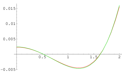
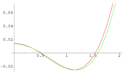
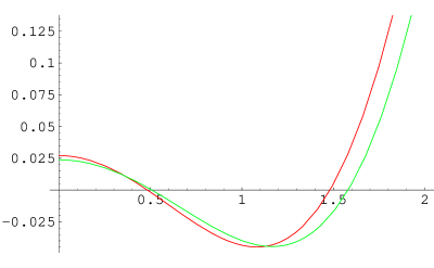
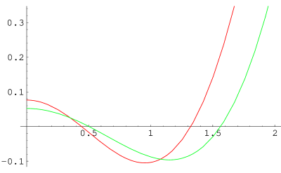
Figure 1: Graphs for $v_{*}(x)$ for $n=2$ from $\varepsilon$-expansion at ${\rm O}(\varepsilon^{2})$ and numerical solution with $v_{*}(0)=-V_{*}^{\prime\prime}(0)/d$ from Table 1 with $d=3.9$, $3.8$, $3.6$, $3.4$, $3.2$, $3.0$.

Similarly we consider the multi-critical fixed points obtained for $n=3$ and $n=4$, which correspond to $\varepsilon$-expansions for dimensions $d=3$ and $d=\frac{8}{3}$ respectively. When $n=3$ the results are

$$k_{3}=\frac{1}{5!^{2}}\,,\qquad{a}_{2p}=\frac{6-p}{3-p}\,\frac{9.2^{7-p}}{p!^{2}(6-p)!}\,,\quad p=0,1,2,4,5\,.$$ (4.9)

Hence

$${a}_{0}=\frac{16}{5}\,,\quad{a}_{2}=12\,,\quad{a}_{4}=12\,,\quad{a}_{8}=-\frac{1}{8}\,,\quad{a}_{10}=-\frac{1}{800}\,.$$ (4.10)

From these, we can determine from (3.24)

$${a}_{6}=\frac{173}{20}\,.$$ (4.11)

At the origin we then obtain

$$v_{*}(0)=-\frac{1}{120}\varepsilon\left(1+\frac{1087}{120}\varepsilon^{2}\right)\,,\qquad v^{\prime\prime}_{*}(0)=\frac{1}{10}\varepsilon\left(1+\frac{389}{40}\varepsilon\right)\,,$$ (4.12)

and hence

$$V_{*}^{\prime\prime}(0)=\frac{1}{40}\varepsilon\left(1+\frac{349}{40}\varepsilon\right)\,.$$ (4.13)

It is easy to verify that $V_{*}^{\prime\prime}(0)/V_{*}(0)=-d$ to this order again. In Table 2 the result (4.13) is compared with the numerical results of [23] in this case and in Figure 2 a graphical comparison of $\varepsilon$-expansion and numerical solutions is made.

$d$	Numerical	$\varepsilon$-expansion at ${\rm O}(\varepsilon^{2})$
3	0	$0\qquad$
2.9	0.005	$0.005\qquad$
2.8	0.015	$0.014\qquad$
2.7	0.032	$0.027\qquad$
2.6	0.062	$0.045\qquad$
2.5	0.108	$0.067\qquad$

Table 2: Comparison of ERG numerical and analytical results for $V_{*}^{\prime\prime}(0)$ for the $n=3$ fixed point.

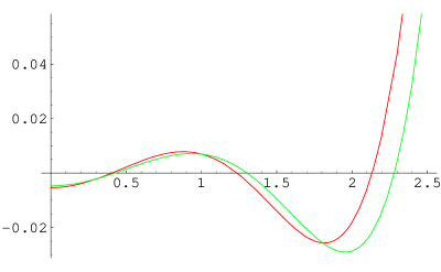
Figure 2: $n=3$ $v_{*}(x)$ from $\varepsilon$-expansion at ${\rm O}(\varepsilon^{2})$ and numerical solution for $d=2.9$, $2.8$ and $2.6$.

Finally, we consider the $n=4$ case. Following the same programme as above, the coefficients in the expansion are

$${a}_{0}= \frac{432}{35}\,,\quad{a}_{2}=\frac{288}{5}\,,\quad{a}_{4}=\frac{324}{5}\,,\quad{a}_{6}=36\,,$$

$${a}_{10}= -\frac{27}{100}\,,\quad{a}_{12}=-\frac{3}{800}\,,\quad{a}_{14}=-\frac{1}{39200}\,,$$ (4.14)

and

$$a_{8}=\frac{23904}{875}\,.$$ (4.15)

The fixed point solution at order $\varepsilon^{2}$ then determines

$$V_{*}^{\prime\prime}(0)=-\frac{3}{560}\varepsilon\left(1+\frac{99441}{3500}\varepsilon\right)\,.$$ (4.16)

Table 3 compares this result with [23] and with some corresponding graphs exhibited in Figure 3.

$d$	Numerical	$\varepsilon$-expansion at ${\rm O}(\varepsilon)$
$\frac{8}{3}$	0	$0\qquad$
2.6	$-0.001$	$-0.001\qquad$
2.5	$-0.008$	$-0.005\qquad$
2.4	$-0.028$	$-0.012\qquad$
2.3	$-0.082$	$-0.022\qquad$
2.2	$-0.226$	$-0.035\qquad$

Table 3: Comparison of ERG numerical and analytical results for $V_{*}^{\prime\prime}(0)$ for the $n=4$ fixed point.

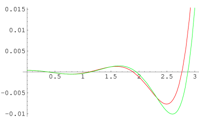
Figure 3: $n=4$ $v_{*}(x)$ from $\varepsilon$-expansion at ${\rm O}(\varepsilon^{2})$ and numerical solution for $d=2.6$, $2.5$ and $2.4$.

5 Critical Exponents

Having computed $v_{*}(x)$ to order $\varepsilon^{2}$ for the fixed points below each critical dimension $d=2n/(n-1)$, we now consider the RG flow near these fixed points and compute certain critical exponents. In the local potential approximation, the ERG flow is given by (3.1) and with the change of variables as in (3.3) we now have the following RG flow equation for $v(x,t)$

$$\frac{4}{d-2}\big{(}\dot{v}(x,t)-dv(x,t)\big{)}=v^{\prime\prime}(x,t)-2xv^{\prime}(x,t)-v^{\prime}(x,t)^{2}\,.$$ (5.1)

In the neighbourhood of a fixed point

$$v(x,t)=v_{*}(x)+e^{\lambda t}f(x)\,,$$ (5.2)

where $f(x)$ therefore satisfies the following linear eigenvalue equation

$$\frac{4}{d-2}(\lambda-d)=f^{\prime\prime}-2xf^{\prime}-2v^{\prime}_{*}f^{\prime}\,.$$ (5.3)

This may be rewritten in the form

$$-Df(x)+v_{*}{\!}^{\prime}(x)f^{\prime}(x)=\hat{\lambda}f(x)\,,\qquad\hat{\lambda}=-\frac{2}{d-2}(\lambda-d)\,,$$ (5.4)

with $D$ the differential operator in (3.6).

In the case of the Gaussian fixed point $v_{*}=0$, the eigenvalues are $\hat{\lambda}_{k}=k$ and the associated eigenfunctions $f_{k}$ are just Hermite polynomials, so that

$$f_{k}(x)=H_{k}(x)\,,\qquad\lambda_{k}=d-{\textstyle\frac{1}{2}}k(d-2)\,,\qquad k=0,1,2,\dots\,.$$ (5.5)

These correspond to the operators $\phi^{k}$ where $\phi$ has dimensions ${\textstyle\frac{1}{2}}(d-2)$. For the high temperature fixed point then in (5.3) $v_{*}^{\prime}(x)=\frac{4}{d-2}x$ and the eigenfunctions are again Hermite polynomials with rescaled variable and $\lambda_{k}=d-{\textstyle\frac{1}{2}}k(d+2)$.

For non trivial critical points we require $v_{*}$ to be a non singular solution of (3.4) For dimension $d$ as in (2.2) we may then consider a perturbation expansion in $\varepsilon$, so that

$$f_{k}(x) =H_{k}(x)+{\rm O}(\varepsilon)\,,$$

$$\hat{\lambda}_{k} =k+\varepsilon\hat{\lambda}_{k}{\!}^{(1)}+\varepsilon^{2}\hat{\lambda}_{k}{\!}^{(2)}+{\rm O}(\varepsilon^{3})\,.$$ (5.6)

To ${\rm O}(\varepsilon)$ it is sufficient to take in (5.4)

$$v_{*}(x)=c_{n}\varepsilon H_{2n}(x)\,.$$ (5.7)

To extract $\hat{\lambda}_{k}{\!}^{(1)}$ we use standard first-order perturbation theory using the basis of eigenfunctions of $D$,

$$N_{k}\hat{\lambda}_{k}{\!}^{(1)} =c_{n}\int_{-\infty}^{\infty}\!\!\!\!{\rm d}x\,e^{-x^{2}}H_{k}(x)H_{2n}{\!}^{\prime}(x)H_{k}{\!}^{\prime}(x)$$

$$=-{\textstyle\frac{1}{2}}c_{n}\int_{-\infty}^{\infty}\!\!\!\!{\rm d}x\,H_{k}(x)^{2}\frac{{\rm d}}{{\rm d}x}\left(e^{-x^{2}}H_{2n}{\!}^{\prime}(x)\right)$$

$$=2nc_{n}\int_{-\infty}^{\infty}\!\!\!\!{\rm d}x\,e^{-x^{2}}H_{k}(x)^{2}H_{2n}(x)$$

$$=2nc_{n}\,G_{kk\,2n}\,.$$ (5.8)

This gives

$$\hat{\lambda}_{k}{\!}^{(1)}=2(n-1)^{2}\frac{n!}{(2n)!}\frac{k!}{(k-n)!}\,,$$ (5.9)

and in terms of the exponents $\lambda_{k}$, we have

$$\lambda_{k} =d-{\textstyle\frac{1}{2}}(d-2)\hat{\lambda}_{k}$$

$$=\frac{2n-k}{n-1}+\varepsilon\left(\frac{1}{2}k-1-2(n-1)\frac{n!}{(2n)!}\frac{k!}{(k-n)!}\right)+{\rm O}(\varepsilon^{2})\,.$$ (5.10)

The results (5.9) or equivalently (5.10) were found in the beginning of the RG analysis of critical points in [24], using an approximation to the Wegner-Houghton RG equation, see also [17], and (up to misprints) in [25], using the LPA for the Wegner-Houghton equation. They are identical with the perturbative result (2.19).

For higher order calculations it is convenient to modify the eigenvalue equation in (5.4) by considering the transformed differential operator

$$\Delta=e^{-v_{*}(x)}\Big{(}-D+v_{*}{\!}^{\prime}(x)\frac{{\rm d}}{{\rm d}x}\Big{)}e^{v_{*}(x)}=-D+\frac{2d}{d-2}\,v_{*}(x)\,,\\$$ (5.11)

using that $v_{*}(x)$ satisfies the fixed point equation (3.4). It is obvious that the eigenvalue equation

$$\Delta{\hat{f}}={\hat{\lambda}}{\hat{f}}\,,$$ (5.12)

is equivalent to (5.4) and furthermore the operator $\Delta$ is hermitian with respect to the measure ${\rm d}x\,e^{-x^{2}}$.

To ${\rm O}(\varepsilon)$ it is easy to see that, with $v_{*}$ given by (5.7) and using the expansion (3.11), that the eigenvalues are the same as (5.9). To ${\rm O}(\varepsilon^{2})$ and using (4.1) second-order perturbation theory gives

$$\hat{\lambda}_{k}{\!}^{(2)} =(n-1)^{2}\frac{c_{n}}{N_{k}}G_{2n\,kk}+\frac{2nc_{n}}{N_{k}}\sum_{p=0}^{2n-1}a_{2p}G_{2p\,kk}-(2nc_{n})^{2}\sum_{m\neq k}\frac{1}{N_{m}N_{k}}\frac{G_{2n\,mk}^{\,2}}{m-k}\,,$$ (5.13)

where the first two terms arise from the ${\rm O}(\varepsilon^{2})$ terms in the operator itself, and the final term is the usual second order perturbation expression for a perturbative potential $2nc_{n}\varepsilon H_{2n}$. Substituting the expressions for $a_{2n}$ and $a_{2p}(p\neq n)$, (3.24) and (3.21) respectively, the expression above becomes

$$\hat{\lambda}_{k}{\!}^{(2)} =\left((n-1)^{2}+n(n-1)\right)\frac{c_{n}}{N_{k}}G_{2n\,kk}-\frac{4n}{(n-1)^{2}}\frac{c_{n}}{N_{2n}}\sum_{p\neq n}\frac{p(2n-p)}{2(n-p)}\frac{G_{2n\,2n\,2p}^{\,2}}{N_{2p}}$$

$$\ \ +2nc_{n}^{2}\sum_{p\neq n}\frac{2n-p}{2(n-p)}\frac{G_{2p\,kk}G_{2n\,2n\,2p}}{N_{2p}N_{k}}-(2nc_{n})^{2}\sum_{m\neq k}\frac{1}{N_{m}N_{k}}\frac{G_{2n\,mk}^{\,2}}{m-k}\,.$$ (5.14)

Finally, substituting for $N_{m}$ from (3.13), $G_{klm}$ from (3.14) and $c_{n}$ from (3.16), we have

$$\hat{\lambda}_{k}{\!}^{(2)} =(n-1)^{3}(2n-1)\frac{1}{n}\frac{n!k!}{(2n)!(k-n)!}$$

$$\ \ -2(n-1)^{4}\frac{1}{n^{2}}\frac{n!^{7}}{(2n)!^{2}}\frac{k!}{(k-n)!}\sum_{p\neq n}\frac{p(2n-p)}{n-p}\frac{(2p)!}{p!^{4}(2n-p)!^{2}}$$

$$\ \ +(n-1)^{4}\frac{1}{n}\frac{n!^{6}}{(2n)!^{2}}k!\sum_{p\neq n}\frac{2n-p}{n-p}\frac{(2p)!}{p!^{4}(k-p)!(2n-p)!}$$

$$\ \ -2(n-1)^{4}\frac{n!^{6}}{(2n)!^{2}}k!\sum_{s\neq n}\frac{1}{n-s}\frac{(2n+k-2s)!}{(k-s)!^{2}s!^{2}(2n-s)!^{2}}\,,$$ (5.15)

where $2s=2n+k-m$. While this expression is somewhat complicated, for any particular choices of $n$ it can be simplified to a polynomial in $k$ of order $2n-1$. Here we give the results for the first two fixed points

$$\hat{\lambda}_{k}{\!}^{(2)}\big{|}_{n=2}= -\frac{1}{12}k(k-1)(k-4)\,,$$ (5.16a)

$$\hat{\lambda}_{k}{\!}^{(2)}\big{|}_{n=3}= -\frac{1}{600}k(k-1)(13k^{3}-17k^{2}-424k+800)\,.$$ (5.16b)

A similar, but not identical result to (5.16a) was obtained in [25], again using the LPA for the Wegner-Houghton RG equation rather than the Polchinski equation.

Having computed the eigenvalues $\hat{\lambda}$ to ${\rm O}(\varepsilon^{2})$, we may now extend (5.10) to calculate the corresponding critical exponents to ${\rm O}(\varepsilon^{2})$. The exponents $\lambda_{k}$ are given in terms of the eigenvalues as

$$\lambda_{k} =\frac{2n-k}{n-1}+\varepsilon\left(\frac{k}{2}-1-2(n-1)\frac{n!}{(2n)!}\frac{k!}{(k-n)!}\right)$$

$$\ \ +\varepsilon^{2}\left((n-1)^{2}\frac{n!}{(2n)!}\frac{k!}{(k-n)!}-\frac{1}{n-1}\hat{\lambda}_{k}{\!}^{(2)}\right)+{\rm O}(\varepsilon^{3})\,.$$ (5.17)

This gives

$$\lambda_{k}\big{|}_{n=2}={} 4-k+\varepsilon\big{(}{\textstyle\frac{1}{2}}k-1-\textstyle{\frac{1}{6}}k(k-1)\big{)}+\varepsilon^{2}\,\textstyle{\frac{1}{12}}k(k-1)(k-3)+{\rm O}(\varepsilon^{3})\,,$$

$$\lambda_{k}\big{|}_{n=3}={} {\textstyle\frac{1}{2}}(6-k)+\varepsilon\big{(}{\textstyle\frac{1}{2}}k-1-\textstyle{\frac{1}{30}}k(k-1)(k-2)\big{)}$$

$${}+\varepsilon^{2}\,\textstyle{\frac{1}{1200}}\,k(k-1)(k-5)(13k^{2}+48k-144)+{\rm O}(\varepsilon^{3})\,.$$ (5.18)

5.1 Exact Exponents

The results (5.9) and (5.16a), (5.16b) show that ${\hat{\lambda}}_{k}=0$ for $k=0,1$ to ${\rm O}(\varepsilon^{2})$, at least for $n=2,3$. For general $n$ from (5.15)

$$\hat{\lambda}_{1}{\!}^{(2)} =(n-1)^{4}\frac{1}{n}\frac{n!^{6}}{(2n)!^{2}}\sum_{p=0}^{1}\frac{2n-p}{n-p}\frac{(2p)!}{p!^{4}(1-p)!(2n-p)!}$$

$$\ \ \ -2(n-1)^{4}\frac{n!^{6}}{(2n)!^{2}}\sum_{s=0}^{1}\frac{1}{n-s}\frac{(2n+1-2s)!}{(1-s)!^{2}s!^{2}(2n-s)!^{2}}$$

$$=2(n-1)^{4}\frac{n!^{6}}{(2n)!^{2}}\frac{1}{n(n-1)(2n)!}\left((n-1)(-2n)+2n(2n-1)-2n^{2}\right)$$

$$=0\,.$$ (5.19)

These results follow in general since it is possible to find exact eigenfunctions for $k=0,1$ in (5.4). Firstly we have the trivial case,

$$f_{0}=1\,,\qquad\hat{\lambda}_{0}=0\,.$$ (5.20)

For $k=1$ we also have

$$f_{1}(x)=v^{\prime}_{*}(x)-\frac{4x}{d-2}\,,\qquad\hat{\lambda}_{1}=1\,.$$ (5.21)

To verify this we first obtain from (3.4)

$$Dv_{*}{\!}^{\prime}+\frac{d+2}{d-2}\,v_{*}{\!}^{\prime}=v_{*}{\!}^{\prime}v_{*}{\!}^{\prime\prime}\,,$$ (5.22)

since then

$$Df_{1}(x)-v_{*}{\!}^{\prime}(x)f_{1}(x)=-v_{*}{\!}^{\prime}(x)+\frac{4x}{d-2}=-f_{1}(x)\,.$$ (5.23)

The vanishing of $\hat{\lambda}_{1}$ reflects that there is no anomalous dimension for the field $\phi$ in the LPA.

Additionally from (5.22) we have another exact eigenfunction and eigenvalue,

$$f_{2n-1}(x)=v^{\prime}_{*}(x)\,,\qquad\hat{\lambda}_{2n-1}=\frac{d+2}{d-2}\,.$$ (5.24)

Expanding the exact eigenvalue $\hat{\lambda}_{2n-1}$ in powers of $\varepsilon$ gives

$$\hat{\lambda}_{2n-1}=2n-1+(n-1)^{2}\varepsilon+{\textstyle\frac{1}{2}}(n-1)^{3}\varepsilon^{2}+\dots\,,$$ (5.25)

which is consistent with (5.9) since

$$\hat{\lambda}^{(1)}_{2n-1}=(n-1)^{2}\,.$$ (5.26)

It is also in accord with the second-order result, (5.15). Relabelling $s=2n-p$,

$$\hat{\lambda}_{2n-1}^{(2)} =(n-1)^{3}(2n-1)\frac{1}{n}\frac{n!(2n-1)!}{(2n)!(n-1)!}$$

$$\ \ \ -2(n-1)^{4}\frac{1}{n^{2}}\frac{n!^{7}}{(2n)!^{2}}\frac{(2n-1)!}{(n-1)!}\sum_{p\neq n}\frac{p(2n-p)}{n-p}\frac{(2p)!}{p!^{4}(2n-p)!^{2}}$$

$$\ \ \ +(n-1)^{4}\frac{1}{n}\frac{n!^{6}}{(2n)!^{2}}(2n-1)!\sum_{p\neq n}\frac{2n-p}{n-p}\frac{(2p)!}{p!^{4}(2n-1-p)!(2n-p)!}$$

$$\ \ \ +2(n-1)^{4}\frac{n!^{6}}{(2n)!^{2}}(2n-1)!\sum_{p\neq n}\frac{1}{n-p}\frac{(2p-1)!}{(p-1)!^{2}p!^{2}(2n-p)!^{2}}$$

$$=\frac{1}{2}(n-1)^{3}+\frac{(n-1)^{4}}{2n^{2}}\frac{n!^{6}}{(2n)!}\sum_{p=0}^{2n}(4n-3p)\frac{(2p)!}{p!^{4}(2n-p)!^{2}}\,.$$ (5.27)

Provided the final sum is identically zero for all $n$ this agrees with the exact result. We demonstrate that the sum vanishes in Appendix B. In this case the relevant operator $\phi^{2n-1}\propto\partial^{2}\phi$ by the equations of motion and has dimension ${\textstyle\frac{1}{2}}(d+2)$.

6 Beyond the Local Potential Approximation

Although the LPA captures the essential features of the fixed point structure in the space of couplings for scalar theories it neglects the momentum dependence of vertices and is therefore limited in terms of calculating critical exponents quantitatively, the anomalous dimension $\eta$ of the scalar field is undetermined and set to zero. Although at the Wilson-Fisher fixed point $\eta$ is small and in the $\varepsilon$-expansion $\eta={\rm O}(\varepsilon^{2})$ it is of course necessary to take $\eta$ into account in more systematic treatments. To this end a natural extension of the LPA is to assume a solution of the exact RG flow equations which is expressible in terms of a local functional of the fields and their derivatives, the derivative expansion [26], for a recent discussion see [27]. In the derivative expansion there is a necessary dependence on the form of the cut off function but in application to the Polchinski RG equation, with terms quadratic in derivatives, there are two constants, see [28, 29].

At the second order in the derivative expansion, the Polchinski equation may be reduced [28] to a following pair of coupled ODEs, extending (3.1), for a potential $V(\phi,t)$ and also the coefficient $Z(\phi,t)$ of ${\textstyle\frac{1}{2}}(\partial\phi)^{2}$ in the derivative expansion,

$$\dot{V} =V^{\prime\prime}-{\textstyle\frac{1}{2}}(d-2+\eta)\phi V^{\prime}+dV-V^{\prime 2}+AZ\,,$$ (6.1a)

$$\dot{Z} =Z^{\prime\prime}-{\textstyle\frac{1}{2}}(d-2+\eta)\phi Z^{\prime}-2V^{\prime}Z^{\prime}-4V^{\prime\prime}Z-\eta Z-\eta+2BV^{\prime\prime 2}\,,$$ (6.1b)

where $A$ and $B$ are the two cut off dependent constants which cannot be eliminated by any rescaling (essentially the same equations were obtained from the Wilson RG equations in [30]).

As earlier it is convenient in our discussion to introduce a rescaled variable

$$x={\textstyle\frac{1}{2}}(d-2+\eta)^{\frac{1}{2}}\phi\,,\qquad v(x,t)=V(\phi,t)\,,\quad z(x,t)=Z(\phi,t),$$ (6.2)

so that the coupled equations (6.1a), (6.1b) become

$$\frac{2}{d-2+\eta}\,\dot{v} =(D+K)v-{\textstyle\frac{1}{2}}\,v^{\prime 2}+\tilde{A}z\,,$$ (6.3a)

$$\frac{2}{d-2+\eta}\,\dot{z} =(D-L)z-v^{\prime}z^{\prime}-2v^{\prime\prime}z-L+{\textstyle\frac{1}{2}}\tilde{B}\,v^{\prime\prime 2}\,,$$ (6.3b)

where

$$K=\frac{2d}{d-2+\eta}\,,\quad L=\frac{2\eta}{d-2+\eta}\,,\qquad\tilde{A}=\frac{2}{d-2+\eta}A\,,\quad\tilde{B}={\textstyle\frac{1}{2}}(d-2+\eta)B\,.$$ (6.4)

At a fixed point, $v(x,t)\to v_{*}(x),\,z(x,t)\to z_{*}(x)$ which satisfy the equations

$$(D+K)v_{*} ={\textstyle\frac{1}{2}}\,v_{*}{\!}^{\prime 2}-\tilde{A}z_{*}\,,\quad$$ (6.5a)

$$(D-L)z_{*}-v_{*}{\!}^{\prime}z_{*}{\!}^{\prime}-2v_{*}{\!}^{\prime\prime}z_{*} =L-{\textstyle\frac{1}{2}}\tilde{B}\,v_{*}{\!}^{\prime\prime 2}\,.$$ (6.5b)

Assuming (2.2) then in an $\varepsilon$-expansion, assuming $A,B$ are $O(1)$, a consistent solution is obtained by requiring $v_{*}(x)={\rm O}(\varepsilon)$ and $\eta,z_{*}(x)={\rm O}(\varepsilon^{2})$. To lowest order then $v_{*}\to\varepsilon c_{n}H_{2n}$ as in (3.10). With this result then (6.5b) becomes

$$Dz_{*}=(n-1)\eta-\varepsilon^{2}{\textstyle\frac{1}{2}}\tilde{B}c_{n}{\!}^{2}H_{2n}{\!\!}^{\prime\prime 2}+{\rm O}(\varepsilon^{3})\,.$$ (6.6)

This determines $\eta=\varepsilon^{2}\,\eta^{(2)}+{\rm O}(\varepsilon^{3})$ since the left hand side of (6.6) is orthogonal to 1 so that

$$(n-1)\eta^{(2)}N_{0}={\textstyle\frac{1}{2}}\tilde{B}c_{n}{\!}^{2}\int^{\infty}_{-\infty}\!\!\!\!{\rm d}x\,e^{-x^{2}}H_{2n}{\!\!}^{\prime\prime 2}\,,$$ (6.7)

which implies

$$\eta^{(2)}=2^{2n+2}\frac{n(2n-1)}{n-1}(2n)!\,\tilde{B}c_{n}{\!}^{2}\,.$$ (6.8)

We consider this further later but first we may then use (6.6) to determine $z_{*}(x)$ to lowest order by using the expansion

$$z_{*}=\varepsilon^{2}c_{n}{\!}^{2}\sum_{p}b_{2p}H_{2p}+{\rm O}(\varepsilon^{3})\,.$$ (6.9)

Since $DH_{2p}=-4pH_{2p}$ and with $H_{2n}{\!\!}^{\prime\prime}=8n(2n-1)H_{2n-2}$ we may obtain

$$b_{2p}={} 16\tilde{B}\,n^{2}(2n-1)^{2}\frac{G_{2p\,2n-2\,2n-2}}{pN_{2p}}$$

$$={} 2^{2n-p}\tilde{B}\frac{(2n)!^{2}}{p(2n-2-p)!p!^{2}}\,,\quad p=1,\dots,2n-2\,.$$ (6.10)

We note that $b_{0}$ is not constrained by (6.6). Nevertheless $b_{0}$ may be determined by imposing $z_{*}(0)=0$ [28]. This ensures that (6.5a), (6.5b) have well defined solutions for all $x$ only for a specific choice of $\eta$ and $v_{*}(0)$.

With these results (6.5a) becomes

$$(D+2n)v_{*}+(n-1)^{2}\varepsilon v_{*}=\varepsilon^{2}c_{n}{\!}^{2}\bigg{(}H_{2n}{\!\!}^{\prime 2}-{\tilde{A}}\sum_{p=0}^{2n-2}b_{2p}H_{2p}\bigg{)}+{\rm O}(\varepsilon^{3})\,,$$ (6.11)

where $v_{*}$ is expressible as in (4.1) and $b_{2p}$ is given by (6.10). Just as in (3.12) and (3.16) this determines normalisation coefficient $c_{n}$,

$$(n-1)^{2}c_{n}N_{2n}=c_{n}{\!}^{2}\big{(}nG_{2n\,2n\,2n}-{\tilde{A}}N_{2n}b_{2n}\big{)}\quad\Rightarrow\quad c_{n}\Big{(}1-\frac{n-1}{n}\,{\tilde{A}}{\tilde{B}}\Big{)}=\frac{(n-1)^{2}}{2^{n}n}\,\frac{n!^{3}}{(2n)!^{2}}\,.$$ (6.12)

Furthermore in (4.1) the expansion coefficients are also determined by (6.11)

$$a_{2p} =c_{n}\frac{1}{2(n-p)}\ \Big{(}(2n-p)\,\frac{G_{2p\,2n\,2n}}{N_{2p}}-{\tilde{A}}\,b_{2p}\Big{)}$$

$$=c_{n}\,\frac{2^{2n-p}}{2(n-p)}\frac{(2n)!^{2}}{p!^{2}(2n-1-p)!}\Big{(}1-\frac{2n-1-p}{p}\,{\tilde{A}}{\tilde{B}}\Big{)}\,,\quad p\neq n\,.$$ (6.13)

except for $a_{2n}$. To obtain this it is necessary to extend (6.11) to ${\rm O}(\varepsilon^{3})$.

Using the result (6.12) the expression (6.8) becomes

$$\eta^{(2)}=4(n-1)^{2}\frac{n!^{6}}{(2n!)^{3}}\,\frac{n(n-1)(2n-1){\tilde{B}}}{\big{(}n-(n-1){\tilde{A}}{\tilde{B}}\big{)}^{2}}\,.$$ (6.14)

The perturbative result (2.19) requires that the final factor, depending on $A,B$, should be one.

7 Critical Exponents with the Derivative Expansion

We now consider small departures from the fixed point of the form

$$v(x,t) =v_{*}(x)+e^{\lambda t}f(x)\,,$$

$$z(x,t) =z_{*}(x)+e^{\lambda t}g(x)\,.$$ (7.1)

Substituting this form into (6.3a), (6.3b) we find the eigenvalue equations

$$-(D+K)f+v_{*}{\!}^{\prime}f^{\prime}-\tilde{A}\,g={} \hat{\lambda}f\,,$$ (7.2a)

$$-(D-L)g+v_{*}{\!}^{\prime}g^{\prime}+2v_{*}{\!}^{\prime\prime}g+z_{*}{\!}^{\prime}f^{\prime}+2z_{*}f^{\prime\prime}-\tilde{B}\,v_{*}{\!}^{\prime\prime}f^{\prime\prime}={} \hat{\lambda}f\,,$$ (7.2b)

with $D$ as in (3.6) and where $\lambda$ is related to $\hat{\lambda}$ according to (this differs from (5.4)).

$$\lambda=-{\textstyle\frac{1}{2}}(d-2+\eta)\hat{\lambda}\,.$$ (7.3)

Defining the vector

$$F=\left(\begin{array}[]{c}f\\ g\\ \end{array}\right)\,,$$ (7.4)

then (7.2a), (7.2b) may be written more compactly in matrix form as

$$\Delta F=\hat{\lambda}F\,.$$ (7.5)

The operator $\Delta$ is not hermitian so for later convenience we also consider the dual equation defining the dual eigenvectors

$${\tilde{\Delta}}\tilde{F}=\hat{\lambda}\tilde{F}\,,$$ (7.6)

where ${\tilde{\Delta}}$ is the adjoint of $\Delta$ with a scalar product defined $\int{\rm d}x\,e^{-x^{2}}\,F_{1}{\!}^{T}F_{2}$.

Just as in Section 5 there are exact eigenfunctions and eigenvalues [28]

$$F={} \left(\begin{array}[]{c}1\\ 0\\ \end{array}\right)\,,\qquad\qquad\qquad\quad\ \ \hat{\lambda}=-K\,,\qquad\ \ \lambda=d\,,$$ (7.7c)

$$F={} \left(\begin{array}[]{c}v_{*}{\!}^{\prime}-(K-2)x\\ z_{*}{\!}^{\prime}\\ \end{array}\right)\,,\qquad\hat{\lambda}=-K+1\,,\quad\lambda={\textstyle\frac{1}{2}}(d+2-\eta)\,,$$ (7.7f)

$$F={} \left(\begin{array}[]{c}v_{*}{\!}^{\prime}\\ z_{*}{\!}^{\prime}\\ \end{array}\right)\,,\qquad\qquad\qquad\quad\,\hat{\lambda}=-1\,,\qquad\quad\,\lambda={\textstyle\frac{1}{2}}(d-2+\eta)\,.$$ (7.7i)

The first corresponds to the identity operator and at the $n$-th multicritical point the second and third to the operators $\phi$ and $\phi^{2n-1}$.

In the $\varepsilon$-expansion

$$\Delta=\Delta^{(0)}+\varepsilon\Delta^{(1)}+\dots\,,$$ (7.8)

and correspondingly in (7.5)

$$\hat{\lambda}=\hat{\lambda}^{(0)}+\varepsilon\hat{\lambda}^{(1)}+\dots\,,\qquad F=F^{(0)}+\varepsilon F^{(1)}+\dots\,,$$ (7.9)

and similarly for $\tilde{F}$. At zeroth order in $\varepsilon$,

$$\Delta^{(0)}=\left(\begin{array}[]{cc}-D-2n&-\tilde{A}\\ 0&-D\\ \end{array}\right)\,.$$ (7.10)

There are two sets of eigenfunctions, which are easily obtained

$$F^{(0)}_{k,1}=\left(\begin{array}[]{c}1\\ 0\\ \end{array}\right)H_{k}\,,\qquad\tilde{F}^{(0)}_{k,1}=\left(\begin{array}[]{c}1\\ \frac{\tilde{A}}{2n}\\ \end{array}\right)H_{k}\,,\qquad k=0,1,2,\dots\,,$$ (7.11)

and

$$F^{(0)}_{k,2}=\left(\begin{array}[]{c}-\frac{\tilde{A}}{2n}\\ 1\\ \end{array}\right)H_{k-2n}\,,\qquad\tilde{F}^{(0)}_{k,2}=\left(\begin{array}[]{c}0\\ 1\\ \end{array}\right)H_{k-2n}\,,\qquad k=2n,2n+1,\dots\,.$$ (7.12)

The eigenvalues in both cases are

$$\hat{\lambda}_{k,1}^{(0)}=\hat{\lambda}_{k,2}^{(0)}=k-2n\,,$$ (7.13)

which are thus two-fold degenerate for $k\geq 2n$.

In general in terms of the perturbative anomalous dimensions at the fixed point discussed in Section 2

$$\lambda_{k,1}=\frac{2n-k}{n-1}-\omega_{k,1}\,,\qquad\lambda_{k,2}=\frac{2n-k}{n-1}-\omega_{k,2}\,.$$ (7.14)

7.1 Eigenvalues at ${\rm O}(\varepsilon)$

We now use first-order perturbation theory to compute $\hat{\lambda}^{(1)}_{k,1}$ and $\hat{\lambda}^{(1)}_{k,2}$. In the expansion (7.8) at ${\rm O}(\varepsilon)$

$$\Delta^{(1)}=\left(\begin{array}[]{cc}-(n-1)^{2}+c_{n}H_{2n}{\!}^{\prime}\frac{{\rm d}}{{\rm d}x}&0\\ -\tilde{B}\,c_{n}H_{2n}{\!\!}^{\prime\prime}\frac{{\rm d}^{2}}{{\rm d}x^{2}}&c_{n}H_{2n}{\!\!}^{\prime}\frac{{\rm d}}{{\rm d}x}+2c_{n}H_{2n}{\!\!}^{\prime\prime}\\ \end{array}\right)\,.$$ (7.15)

The ${\rm O}(\varepsilon)$ results are determined in terms of the $2\times 2$ matrix ${\cal M}_{k}$ defined by

$${\cal M}_{k,ij}=\int_{-\infty}^{\infty}\!\!\!\!{\rm d}x\,e^{-x^{2}}\tilde{F}^{(0)\,T}_{k,i}\,\Delta^{(1)}F^{(0)}_{k,j}\,.$$ (7.16)

For $k<2n$ there is a single eigenfunction so that the perturbation theory result is just

$$N_{k}\hat{\lambda}^{(1)}_{k,1} ={\cal M}_{k,11}$$

$$=-(n-1)^{2}N_{k}+c_{n}\int_{-\infty}^{\infty}\!\!\!\!{\rm d}x\,e^{-x^{2}}H_{k}H_{2n}{\!\!}^{\prime}H_{k}{\!}^{\prime}-c_{n}\frac{1}{2n}\tilde{A}\tilde{B}\int_{-\infty}^{\infty}\!\!\!\!{\rm d}x\,e^{-x^{2}}H_{k}H_{2n}{\!\!}^{\prime\prime}H_{k}{\!}^{\prime\prime}\,.$$ (7.17)

Hence, using the formulae for $N_{k}$, $G_{klm}$ in (3.13), (3.14) we obtain

$$\hat{\lambda}^{(1)}_{k,1}={} -(n-1)^{2}+c_{n}\,2^{n+1}\frac{(2n)!k!}{n!^{2}(k-n)!}\big{(}n-(n-1)\tilde{A}\tilde{B}(n-1)\big{)}$$

$$={} -(n-1)^{2}+2(n-1)^{2}\frac{n!}{(2n)!}\frac{k!}{(k-n)!}\,,$$ (7.18)

where $c_{n}$ is determined by (6.12) so that the dependence on $\tilde{A},\tilde{B}$ disappears. This result is essentially identical to (5.9) and is in accord with the exact results (7.7c), (7.7f), (7.7i) which correspond to $k=0,1,2n-1$.

For $k\geq 2n$ there is a two-fold degeneracy, and so we use degenerate perturbation theory. In particular, for non-trivial first-order eigenfunctions we require that the first-order perturbations to the eigenvalues solve the following characteristic equation

$$\det\big{[}\lambda^{(1)}_{k}{\cal N}_{k}-{\cal M}_{k}\big{]}=0\,,$$ (7.19)

where the ${\cal N}_{k}$ is the diagonal matrix

$${\cal N}_{k}=\left(\begin{array}[]{cc}N_{k}&0\\ 0&N_{k-2n}\\ \end{array}\right)\,,$$ (7.20)

More explicitly, the elements of $\cal M$ are given by (7.17) and

$${\cal M}_{k,22} =c_{n}\int_{-\infty}^{\infty}\!\!\!\!{\rm d}x\,e^{-x^{2}}H_{k-2n}^{\vphantom{T}}\left(H^{\prime}_{2n}H^{\prime}_{k-2n}+2H^{\prime\prime}_{2n}H_{k-2n}+\frac{1}{2n}\tilde{A}\tilde{B}\,H^{\prime\prime}_{2n}H^{\prime\prime}_{k-2n}\right)\,,$$ (7.21a)

$${\cal M}_{k,21} =-\tilde{B}\,c_{n}\int_{-\infty}^{\infty}\!\!\!\!{\rm d}x\,e^{-x^{2}}H_{k-2n}^{\vphantom{T}}H^{\prime\prime}_{2n}H^{\prime\prime}_{k},$$ (7.21b)

$${\cal M}_{k,12} =c_{n}\frac{1}{2n}\tilde{A}\int_{-\infty}^{\infty}{\rm d}x\,e^{-x^{2}}H_{k}^{\vphantom{T}}\left(2H^{\prime\prime}_{2n}H_{k-2n}^{\vphantom{T}}+\frac{1}{2n}\tilde{A}\tilde{B}H^{\prime\prime}_{2n}H^{\prime\prime}_{k-2n}\right)$$

$$=0\,,$$ (7.21c)

where in (7.21c) we use that $H_{k}$ is orthogonal to polynomials of degree $<k$. Hence since the matrix ${\cal M}_{k}$ is lower triangular the eigenvalues solving (7.19) are just $\hat{\lambda}^{(1)}_{1,k}$ as in (7.18) and

$$\hat{\lambda}^{(1)}_{k,2}={} \frac{{\cal M}_{k,22}}{N_{k-2n}}=c_{n}\,2^{n+1}\frac{(2n)!(k-2n)!}{n!^{2}(k-3n+1)!}\left(n(k-n+1)+\tilde{A}\tilde{B}(n-1)(k-3n+1)\right)\,.$$ (7.22)

From (7.3) $\lambda=-(\frac{1}{n-1}-{\textstyle\frac{1}{2}}\varepsilon){\hat{\lambda}}+{\rm O}(\varepsilon^{2})$ so to ${\rm O}(\varepsilon)$ we then have

$$\lambda_{k,1}={} \frac{2n-k}{n-1}+\varepsilon\left[\frac{1}{2}k-1-2(n-1)\frac{n!\,k!}{(2n)!\,(k-n)!}\right]\,,$$ (7.23a)

$$\lambda_{k,2}={} \frac{2n-k}{n-1}$$

$$\!{}+\varepsilon\left[\frac{1}{2}k-n-2(n-1)\frac{n!\,(k-2n)!}{(2n)!\,(k-3n+1)!}\frac{n(k-n+1)+(n-1)\tilde{A}\tilde{B}(k-3n+1)}{n-(n-1)\tilde{A}\tilde{B}}\right]\,.$$ (7.23b)

The result (7.23a) matches the perturbative result in (2.27) but (7.23b) depends on $AB$ so cannot agree with (2.44) in general.

8 Expansion of Exact RG Equation

An alternative approach, which nevertheless has many similarities although some crucial differences to the derivative expansion, is to expand the full renormalisation group equation which contains linear and quadratic terms in terms of translation invariant operators, or scaling fields, which are exact eigen-solutions for its linearised part. This has been applied in [17] and [31], [32] to the Wilson RG equation. Here we apply similar methods more simply to the Polchinski equation for the effective action $S[\varphi,t]$ for a scalar field $\varphi$. This takes the form, after convenient rescalings by the cut off scale $\Lambda$, $t=-\ln\Lambda$,

$$\frac{\partial}{\partial t}S={} \frac{1}{(2\pi)^{d}}\int{\rm d}^{d}p\,\big{(}{\textstyle\frac{1}{2}}d+1-{\textstyle\frac{1}{2}}\eta+p\cdot\partial_{p}\big{)}\tilde{\varphi}(p)\frac{\delta S}{\delta\tilde{\varphi}(p)}$$

$${}-\frac{1}{(2\pi)^{d}}\int{\rm d}^{d}p\,K^{\prime}(p^{2})\bigg{(}\frac{\delta^{2}S}{\delta\tilde{\varphi}(p)\delta\tilde{\varphi}(-p)}-\frac{\delta S}{\delta\tilde{\varphi}(p)}\,\frac{\delta S}{\delta\tilde{\varphi}(-p)}\bigg{)}$$

$${}-{\textstyle\frac{1}{2}}\eta\,\frac{1}{(2\pi)^{d}}\int{\rm d}^{d}p\,K(p^{2})^{-1}p^{2}\tilde{\varphi}(p)\tilde{\varphi}(-p)+C\,,$$ (8.1)

where $K(p^{2}/\Lambda^{2})$ is a cut off function and $\tilde{\varphi}$ is the Fourier transform of $\varphi$, $\delta\tilde{\varphi}(p)/\delta\tilde{\varphi}(p^{\prime})=(2\pi)^{d}\delta^{d}(p-p^{\prime})$. $C$ is an additional constant independent of $\varphi$, in general it is irrelevant and may be neglected. Apart from $K(0)=1$ and sufficient rapid fall off for large $p^{2}$ no restriction on the cut off function $K(p^{2})$ is imposed here. The Gaussian fixed point corresponds to $S=0$ and also when the anomalous scale dimension for $\varphi$, $\eta=0$. The appearance of $\eta$ in (8.1) arises by assuming that $\varphi$ varies with the cut off $\Lambda$ with an anomalous dimension ${\textstyle\frac{1}{2}}\eta$. As will be apparent later the additional term proportional to $\eta$ in (8.1) is necessary for consistent RG flow solutions. The derivative expansion is obtained directly by approximating (8.1) by assuming $\tilde{\varphi}(p)$ is expanded as $(2\pi)^{d}(\phi-i\partial\phi\cdot\partial_{p})\delta^{d}(p)$ and requiring $S[\varphi,t]\to\int{\rm d}^{d}x\big{(}V(\phi,t)+{\textstyle\frac{1}{2}}Z(\phi,t)(\partial\phi)^{2}\big{)}$.

The starting point of the discussion in this Section requires solutions of

$$\big{(}{\cal D}_{1}+{\cal D}_{2}\big{)}{\cal O}=\lambda{\cal O}\,,$$ (8.2)

for ${\cal D}_{1}+{\cal D}_{2}$ the differential operator defined by the linear part of (8.1),

$${\cal D}_{1}={} \frac{1}{(2\pi)^{d}}\int{\rm d}^{d}p\,\big{(}{\textstyle\frac{1}{2}}d+1+p\cdot\partial_{p}\big{)}\tilde{\varphi}(p)\,\frac{\delta}{\delta\tilde{\varphi}(p)}\,,$$

$${\cal D}_{2}={} -\frac{1}{(2\pi)^{d}}\int{\rm d}^{d}p\,K^{\prime}(p^{2})\frac{\delta^{2}}{\delta\tilde{\varphi}(p)\delta\tilde{\varphi}(-p)}\,.$$ (8.3)

The eigenvalue equation

$${\cal D}_{1}{\hat{\cal O}}=\lambda{\hat{\cal O}}\,,$$ (8.4)

is easily solved in terms of local translational invariant operators by

$${\hat{\cal O}}=\frac{1}{(2\pi)^{d(k-1)}}\int\prod_{i=1}^{k}{\rm d}^{d}p_{i}\,\tilde{\varphi}(p_{i})\ \delta^{d}\big{(}{\textstyle\sum_{i}}p_{i}\big{)}\,O(p_{1},\dots,p_{k})\,,\quad\lambda=d-k({\textstyle\frac{1}{2}}d-1)-r\,,$$ (8.5)

where $O(p_{1},\dots,p_{k})$ is a scalar symmetric homogeneous polynomial of degree $r$. We then obtain corresponding solutions of (8.2) in the form

$${\cal O}=e^{-{\cal Y}}{\hat{\cal O}}\,,$$ (8.6)

where ${\cal Y}$ is defined by

$$[{\cal D}_{1},{\cal Y}]={\cal D}_{2}\,,$$ (8.7)

ensuring that ${\cal O}$ as defined by (8.6) has the same eigenvalue as $\hat{\cal O}$. It is easy to solve (8.7) giving

$${\cal Y}={\textstyle\frac{1}{2}}\,\frac{1}{(2\pi)^{d}}\int{\rm d}^{d}p\ G(p)\,\frac{\delta^{2}}{\delta\tilde{\varphi}(p)\delta\tilde{\varphi}(-p)}\,,\qquad G(p)=\frac{K(p^{2})}{p^{2}}\,,$$ (8.8)

so that in (8.6) $e^{-{\cal Y}}$ essentially generates normal ordering.

For comparison with the derivative expansion earlier we consider just operators with $r=0,2$ for which a convenient basis is

$${\cal O}_{k0}={} e^{-{\cal Y}}\frac{1}{(2\pi)^{d(k-1)}}\int\prod_{i=1}^{k}{\rm d}^{d}p_{i}\,\tilde{\varphi}(p_{i})\ \delta^{d}\big{(}p_{(k)}\big{)}\,,\qquad p_{(k)}={\textstyle\sum_{i=1}^{k}}\,p_{i}\,,$$

$${\cal O}_{k2}={} \frac{1}{k(k-1)}\,e^{-{\cal Y}}\,\frac{1}{(2\pi)^{d(k-1)}}\int\prod_{i=1}^{k}{\rm d}^{d}p_{i}\,\tilde{\varphi}(p_{i})\ \delta^{d}\big{(}p_{(k)}\big{)}\,\sum_{i=1}^{k}p_{k}{\!}^{2}\,,\quad k=2,3,\dots\,.$$ (8.9)

The result for ${\cal O}_{k0}$ may be expressed in terms of Hermite polynomial as a consequence of the identity

$$e^{-\frac{1}{4}\,\frac{{\rm d}^{2}}{{\rm d}x^{2}}}(2x)^{n}=H_{n}(x)\,.$$ (8.10)

The nonlinear term in (8.1) may be evaluated in terms operators ${\cal O}$ and ${\cal O}^{\prime}$, respectively of degree $l$ and $m$ in $\tilde{\varphi}$ and as given by (8.5) and (8.6), by considering [17]

$$e^{{\cal Y}}\frac{1}{(2\pi)^{d}}\int{\rm d}^{d}p\,K^{\prime}(p^{2})\,\frac{\delta{\cal O}}{\delta\tilde{\varphi}(p)}\,\frac{\delta{\cal O}^{\prime}}{\delta\tilde{\varphi}(-p)}$$

$${}=\exp\bigg{(}\frac{1}{(2\pi)^{d}}\!\int\!{\rm d}^{d}p\,G(p)\,\frac{\delta^{2}}{\delta\tilde{\varphi}(p)\delta\tilde{\varphi}^{\prime}(-p)}\bigg{)}\,lm\frac{1}{(2\pi)^{d(l+m-3)}}\!\int\prod_{i=1}^{l-1}{\rm d}^{d}p_{i}\,\tilde{\varphi}(p_{i})\!\int\prod_{j=1}^{m-1}{\rm d}^{d}q_{j}\,\tilde{\varphi}^{\prime}(q_{j})$$

$${}\!\quad\times\delta^{d}\big{(}p_{(l-1)}+q_{(m-1)}\big{)}\ O\big{(}p_{1},\dots,p_{l-1},-p_{(l-1)}\big{)}\,O^{\prime}\big{(}q_{1},\dots,q_{m-1},-q_{(m-1)}\big{)}\Big{|}_{\tilde{\varphi}^{\prime}=\tilde{\varphi}}\,K^{\prime}\big{(}p_{(l-1)}{\!\!}^{2}\big{)}$$

$${}=\sum_{n\geq 0}\frac{l!\,m!}{n!(l-1-n)!(m-1-n)!}\,\frac{1}{(2\pi)^{d(l+m-3-2n)}}\int\prod_{i=1}^{l-1-n}\!\!\!{\rm d}^{d}p_{i}\,\tilde{\varphi}(p_{i})\,\int\prod_{j=1}^{m-1-n}\!\!\!{\rm d}^{d}q_{j}\,\tilde{\varphi}(q_{j})\,$$

$${}\qquad\times\delta^{d}\big{(}p_{(l-1-n)}+q_{(m-1-n)}\big{)}\,F_{n}(p_{1},\dots,p_{l-1-n};q_{1},\dots,q_{m-1-n})\,,$$ (8.11)

where, with $p_{(l-1-n)}+q_{(m-1-n)}=0$,

$${}F_{n}(p_{1},\dots,p_{l-1-n};q_{1},\dots,q_{m-1-n})$$

$${}=\frac{1}{(2\pi)^{dn}}\int\prod_{h=1}^{n}{\rm d}^{d}r_{h}\,G(r_{h})\,O\big{(}p_{1},\dots,p_{l-1-n},r_{n},\dots,r_{1},-p_{(l-1-n)}-r_{(n)}\big{)}$$

$$\quad\quad{}\times O^{\prime}\big{(}q_{1},\dots,q_{m-1-n},-r_{n},\dots,-r_{1},-q_{(m-1-n)}-r_{(n)}\big{)}\,K^{\prime}\big{(}(p_{(l-1-n)}+r_{(n)})^{2}\big{)}\,.$$ (8.12)

For the cases of interest here

$$\hskip-14.22636pt{\cal O}={\cal O}_{l0}\,,\quad{\cal O}^{\prime}={\cal O}_{m0}\,,$$

$$\hskip-14.22636ptF_{n}(p_{1},\dots,p_{l-1-n};q_{1},\dots,q_{m-1-n})=\rho_{n}\big{(}p_{(l-1-n)}{\!}^{2}\big{)}\,,$$

$$\hskip-14.22636pt{\cal O}={\cal O}_{l0}\,,\quad{\cal O}^{\prime}={\cal O}_{m2}\,,$$

$$\hskip-14.22636ptF_{n}(p_{1},\dots,p_{l-1-n};q_{1},\dots,q_{m-1-n})={\textstyle{\sum_{j=1}^{m-1-n}\!q_{j}{\!}^{2}}}\,\rho_{n}\big{(}p_{(l-1-n)}{\!}^{2}\big{)}+\tau_{n}\big{(}p_{(l-1-n)}{\!}^{2}\big{)}\,,$$ (8.13)

with

$$\rho_{n}(p^{2})={} \frac{1}{(2\pi)^{dn}}\int\prod_{h=1}^{n}{\rm d}^{d}r_{h}\,G(r_{h})\,K^{\prime}\big{(}(p+r_{(n)})^{2}\big{)}\,,$$ (8.14a)

$$\tau_{n}(p^{2})={} \frac{1}{(2\pi)^{dn}}\int\prod_{h=1}^{n}{\rm d}^{d}r_{h}\,G(r_{h})\,\big{(}n\,r_{n}{\!}^{2}+(p+r_{(n)})^{2}\big{)}\,K^{\prime}\big{(}(p+r_{(n)})^{2}\big{)}\,.$$ (8.14b)

With the aid of (8.11) and (8.13) we may then write

$$\frac{1}{(2\pi)^{d}}\int{\rm d}^{d}p\,K^{\prime}(p^{2})\,\frac{\delta{\cal O}_{l0}}{\delta\tilde{\varphi}(p)}\frac{\delta{\cal O}_{m0}}{\delta\tilde{\varphi}(-p)}=\sum_{k}\big{(}{\cal O}_{k0}\,C_{klm}+{\cal O}_{k2}\,{\tilde{C}}_{klm}+\dots\big{)}\,,$$

$$\frac{1}{(2\pi)^{d}}\int{\rm d}^{d}p\,K^{\prime}(p^{2})\,\frac{\delta{\cal O}_{l0}}{\delta\tilde{\varphi}(p)}\frac{\delta{\cal O}_{m2}}{\delta\tilde{\varphi}(-p)}=\sum_{k}\big{(}{\cal O}_{k0}\,D_{klm}+{\cal O}_{k2}\,{\tilde{D}}_{klm}+\dots\big{)}\,,$$ (8.15)

for

$$C_{klm}={} \frac{l!\,m!}{(s-1-k)!(s-l)!(s-m)!}\,\rho_{s-1-k}(0)\,,$$

$${\tilde{C}}_{klm}={} \frac{l!\,m!}{(s-1-k)!(s-1-l)!(s-1-m)!}\,\rho^{\prime}{\!}_{s-1-k}(0)\,,$$

$$D_{klm}={} \frac{l!\,(m-2)!}{(s-1-k)!(s-l)!(s-m)!}\,\tau_{s-1-k}(0)\,,$$

$${\tilde{D}}_{klm}={} \frac{l!\,(m-2)!}{(s-1-k)!(s-1-l)!(s-m)!}\,\big{(}(k-1)\rho_{s-1-k}(0)+\tau^{\prime}{\!}_{s-1-k}(0)\big{)}\,,$$ (8.16)

which are non zero so long as $s={\textstyle\frac{1}{2}}(k+l+m)=k+1,k+2,\dots$.

The truncation of the full RG equation (8.1) corresponding to the derivative expansion as considered in Section 6 is obtained by writing

$$S=\textstyle{\sum_{k}}\big{(}a_{k}\,{\cal O}_{k0}+b_{k}\,{\cal O}_{k2}\big{)}\,,$$ (8.17)

and then reducing (8.1) to

$${\dot{a}}_{k}={} \big{(}d-{\textstyle\frac{1}{2}}(d-2+\eta)k\big{)}\,a_{k}+\textstyle{\sum_{l,m}\big{(}C_{klm}\,a_{l}a_{m}+2D_{klm}\,a_{l}b_{m}}\big{)}\,,$$ (8.18a)

$${\dot{b}}_{k}={} \big{(}d-2-{\textstyle\frac{1}{2}}(d-2+\eta)k\big{)}\,b_{k}-{\textstyle\frac{1}{2}}\eta\,\delta_{k2}+\textstyle{\sum_{l,m}\big{(}{\tilde{C}}_{klm}\,a_{l}a_{m}+2{\tilde{D}}_{klm}\,a_{l}b_{m}}\big{)}\,.$$ (8.18b)

These equations are arbitrary up to the rescalings

$$a_{k}\to a_{k}/\alpha_{k}\,,\ b_{k}\to b_{k}/\beta_{k}\,,\quad C_{klm}\to{} C_{klm}\alpha_{l}\alpha_{m}/\alpha_{k}\,,\quad D_{klm}\to D_{klm}\alpha_{l}\beta_{m}/\alpha_{k}\,,$$

$${\tilde{C}}_{klm}\to{} {\tilde{C}}_{klm}\alpha_{l}\alpha_{m}/\beta_{k}\,,\quad{\tilde{D}}_{klm}\to{\tilde{D}}_{klm}\alpha_{l}\beta_{m}/\beta_{k}\,,$$ (8.19)

for any $\alpha_{k},\beta_{k}$ so long as $\beta_{2}=1$ because of the inhomogeneous $\eta$ term in (8.18b). Deferring further discussion to later we may impose $b_{2}=0$. Letting $\alpha_{k}=u^{\frac{1}{2}k-1}v$, $\beta_{k}=u^{\frac{1}{2}k-1}$ then these rescalings correspond to changes in the cut off dependent functions in (8.16) of the form

$$\rho_{n}(0)\to u^{n}v\,\rho_{n}(0)\,,\quad\rho^{\prime}{\!}_{n}(0)\to u^{n}v^{2}\,\rho^{\prime}{\!}_{n}(0)\,,\quad\tau_{n}(0)\to u^{n}\,\tau_{n}(0)\,,\quad\tau^{\prime}{\!}_{n}(0)\to u^{n}v\,\tau^{\prime}{\!}_{n}(0)\,.$$ (8.20)

Critical exponents calculated from (8.18a),(8.18b) must be independent of such transformations.

The analysis of (8.18a),(8.18b) in the $\varepsilon$-expansion, with $d$ as in (2.2), is very similar to the previous discussion in the context of the derivative expansion. At a fixed point a consistent solution is obtained with

$$a_{*k}=\varepsilon\,a_{*}\delta_{k\,2n}+\varepsilon^{2}\,a_{*k}{\!}^{(2)}+{\rm O}(\varepsilon^{3})\,,\quad b_{*k}=\varepsilon^{2}\,b_{*k}{\!}^{(2)}+{\rm O}(\varepsilon^{3})\,,\qquad\eta=\varepsilon^{2}\,\eta^{(2)}+{\rm O}(\varepsilon^{3})\,,$$ (8.21)

where

$$a_{*}={} -\frac{n-1}{C_{2n\,2n\,2n}}\,,\qquad\quad\eta^{(2)}=2a_{*}{\!}^{2}{\tilde{C}}_{2\,2n\,2n}\,,$$

$$b_{*2p}{\!}^{(2)}={} \frac{n-1}{2(p-1)}\,a_{*}{\!}^{2}{\tilde{C}}_{2p\,2n\,2n}\,,\ p\neq 1\,,\qquad a_{*2p}{\!}^{(2)}=\frac{n-1}{2(p-n)}\,a_{*}{\!}^{2}{C}_{2p\,2n\,2n}\,,\ p\neq n\,,$$

$$a_{*2n}{\!}^{(2)}={} -\frac{2a_{*}}{n-1}\Big{(}{\textstyle{\sum_{p\neq n}}}C_{2n\,2n\,2p}\,a_{*2p}{\!}^{(2)}+{\textstyle{\sum_{p\neq 1}}}D_{2n\,2n\,2p}\,b_{*2p}{\!}^{(2)}\Big{)}\,.$$ (8.22)

Hence with (8.16) this gives

$$\eta^{(2)}=4(n-1)^{2}\frac{n!^{6}}{(2n)!^{3}}\,\frac{2n-1}{n}\,\frac{\rho^{\prime}{\!}_{2n-1}(0)}{\rho_{n-1}(0)^{2}}\,.$$ (8.23)

In general $\rho_{n}$, and also $\tau_{n}$, as defined in (8.14a) and (8.14b) depend on the cut off function but as shown in Appendix C there are certain universal quantities which are related to logarithmic divergences. In particular

$$\frac{\rho^{\prime}{\!}_{2n-1}(0)}{\rho_{n-1}(0)^{2}}\bigg{|}_{d=d_{n}}=\frac{n}{2n-1}=\frac{d_{n}}{d_{n}+2}\,,$$ (8.24)

so that (8.23) is in exact accord with (2.19).

In the neighbourhood of a fixed point the solutions of (8.18a), (8.18b) are written as

$$a_{k}(t)=a_{*k}+e^{\lambda t}f_{k}\,,\qquad b_{k}(t)=b_{*k}+e^{\lambda t}g_{k+2(n-1)}\,,$$ (8.25)

for $f_{k},g_{k+2(n-1)}$ small. The critical exponents are then determined by the linear eigenvalue equation

$$\frac{2n-k}{n-1}\,\left(\begin{array}[]{cc}f_{k}\\ g_{k}\\ \end{array}\right)+\sum_{l}\left(\begin{array}[]{cc}{\cal M}_{11,kl}&{\cal M}_{12,kl}\\ {\cal M}_{21,kl}&{\cal M}_{22,kl}\\ \end{array}\right)\left(\begin{array}[]{cc}f_{l}\\ g_{l}\\ \end{array}\right)=\lambda\left(\begin{array}[]{cc}f_{k}\\ g_{k}\\ \end{array}\right)\,,$$ (8.26)

for

$${\cal M}_{11,kl}={} \big{(}\varepsilon({\textstyle\frac{1}{2}}k-1)-{\textstyle\frac{1}{2}}k\eta\big{)}\delta_{kl}+2{\textstyle{\sum_{m}}}\big{(}C_{klm}\,a_{*m}+D_{klm}\,b_{*m}\big{)}\,,$$

$${\cal M}_{22,kl}={} \big{(}\varepsilon({\textstyle\frac{1}{2}}k-n)-({\textstyle\frac{1}{2}}k-n+1)\eta\big{)}\delta_{kl}+2{\textstyle{\sum_{m}}}{\tilde{D}}_{k-2(n-1)\ m\ l-2(n-1)}\,a_{*m}^{\vphantom{g}}\,,$$

$${\cal M}_{12,kl}={} 2{\textstyle{\sum_{m}}}D_{km\ l-2(n-1)}\,a_{*m}^{\vphantom{g}}\,,$$

$${\cal M}_{21,kl}={} 2{\textstyle{\sum_{m}}}\big{(}{\tilde{C}}_{k-2(n-1)\ lm}\,a_{*m}^{\vphantom{g}}+{\tilde{D}}_{k-2(n-1)\ lm}\,b_{*m}^{\vphantom{g}}\big{)}\,.$$ (8.27)

To first order in $\varepsilon$ we may let $a_{*m}\to\varepsilon\,a_{*}\delta_{m\,2n}$ and $b_{*m}\to 0$. Since

$$D_{k\,2n\,k-2(n-1)}=\frac{2n}{k+1-2n}\,\tau_{0}(0)=0\,,$$ (8.28)

as from (8.14b) $\tau_{0}(p^{2})=p^{2}K^{\prime}(p^{2})$, then ${\cal M}_{12,kl}$ is ${\rm O}(\varepsilon^{2})$, whereas otherwise ${\cal M}_{11,kl},{\cal M}_{21,kl}$ and ${\cal M}_{22,kl}$ are ${\rm O}(\varepsilon)$. Hence the first order critical exponents from (8.26) are

$$\lambda_{1,k}{\!}^{(1)}={} {\textstyle\frac{1}{2}}k-1+2a_{*}\,C_{kk\,2n}={\textstyle\frac{1}{2}}k-1-2(n-1)\frac{n!\,k!}{(2n)!\,(k-n)!}\,,$$

$$\lambda_{2,k}{\!}^{(1)}={} {\textstyle\frac{1}{2}}k-n+2a_{*}\,{\tilde{D}}_{k-2(n-1)\ 2n\ k-(2(n-1)}$$

$$={} {\textstyle\frac{1}{2}}k-n-2(n-1)\frac{n!\,(k-2n)!}{(2n)!\,(k-3n+1)!}\bigg{(}k-2n+1+n\,\frac{\tau^{\prime}{\!}_{n-1}(0)}{\rho_{n-1}(0)}\bigg{)}\,.$$ (8.29)

Just as in (8.24)

$$\tau^{\prime}{\!}_{n-1}(0)\big{|}_{d=d_{n}}=0\,,$$ (8.30)

so that (8.29) is in exact agreement with the perturbative results (2.27) and (2.44).

9 Modified Derivative Expansion

The results of Section 8 can be rewritten in a form which is close to the derivative expansion. To achieve this it is necessary to make specific choices of the cut off dependent quantities which appear in (8.16) and which are arbitrary up to the freedom exhibited in (8.20). It is crucial of course that the cut-off function independent results in (8.24) and (8.30), as well as $\tau_{0}(0)=0$, should be satisfied. To this end we choose

$$\rho_{n}(0)=-1\,,\qquad\rho^{\prime}{\!}_{n}(0)=\frac{d}{d+2}\,,\qquad\tau_{n}(0)={\cal A}n\,,\qquad\tau^{\prime}{\!}_{n}(0)=0\,,$$ (9.1)

where ${\cal A}$ is arbitrary. With these choices, and with (3.13) and (3.14), then (8.16) gives

$$C_{klm}={} -2^{\frac{1}{2}(k-l-m)+1}\,\frac{1}{N_{k}}\,lm\,G_{k\,l-1\,m-1}\,,$$

$${\tilde{C}}_{k+2\,lm}={} \frac{d}{d+2}\,2^{\frac{1}{2}(k-l-m)+2}\,\frac{1}{N_{k}}\,l(l-1)m(m-1)\,G_{k\,l-2\,m-2}\,,$$

$$D_{kl\,m+2}={} {\cal A}\,2^{\frac{1}{2}(k-l-m)+1}\,\frac{1}{N_{k}}\,l(l-1)G_{k\,l-2\,m}\,,$$

$${\tilde{D}}_{k+2\,l\,m+2}={} -2^{\frac{1}{2}(k-l-m)+1}\,\frac{1}{N_{k}}\,\big{(}lm\,G_{k\,l-1\,m-1}+l(l-1)\,G_{k\,l-2\,m}\big{)}\,.$$ (9.2)

If we now define

$${\tilde{v}}(x)=\sum_{k}a_{k}\,2^{-\frac{1}{2}k}H_{k}(x)\,,\qquad{\tilde{z}}(x)=\sum_{k}b_{k+2}\,2^{-\frac{1}{2}k}H_{k}(x)\,,$$ (9.3)

then the truncated RG equations (8.18a) and (8.18b) are equivalent, subject to requiring non singular solutions for all $x$, to the coupled differential equations

$${\dot{\tilde{v}}}={} \big{(}d+{\textstyle\frac{1}{2}}(d-2+\eta)D\big{)}\tilde{v}-{\textstyle\frac{1}{2}}\,\tilde{v}^{\prime}{}^{2}+{\cal A}\,\tilde{v}^{\prime\prime}\tilde{z}\,,$$ (9.4a)

$${\dot{\tilde{z}}}={} \big{(}-\eta+{\textstyle\frac{1}{2}}(d-2+\eta)D\big{)}\tilde{z}-\tilde{v}^{\prime}\tilde{z}^{\prime}-\tilde{v}^{\prime\prime}\tilde{z}-{\textstyle\frac{1}{2}}\eta+\frac{d}{4(d+2)}\,\tilde{v}^{\prime\prime}{}^{2}\,.$$ (9.4b)

With the redefinitions

$$v=\frac{2}{d-2+\eta}\,\tilde{v}\,,\qquad z=2\tilde{z}\,,$$ (9.5)

and, with $K,L$ defined as in (6.4), then these become

$$\frac{2}{d-2+\eta}\,{\dot{v}}={} (D+K)v-{\textstyle\frac{1}{2}}\,v^{\prime}{}^{2}+{\tilde{\cal A}}\,v^{\prime\prime}z\,,$$ (9.6a)

$$\frac{2}{d-2+\eta}\,{\dot{z}}={} (D-L)z-v^{\prime}z^{\prime}-v^{\prime\prime}z-L+{\textstyle\frac{1}{2}}{\tilde{\cal B}}\,v^{\prime\prime}{}^{2}\,,$$ (9.6b)

for

$${\tilde{\cal A}}=\frac{2}{d-2+\eta}\,{\cal A}\,,\qquad{\tilde{\cal B}}={\textstyle\frac{1}{2}}(d-2+\eta)\,\frac{d}{d+2}\,.$$ (9.7)

The results (9.6a) and (9.6b) are very similar to (6.3a) and (6.3b), although there is no linear $z$ term in (9.6a) and the coefficient ${\tilde{\cal B}}$ is determined in (9.6b). As a consequence the coefficient $c_{n}$ in the leading order solution (3.10) is unchanged from (3.16). Furthermore following the same discussion as in Sections 6 and 7 gives the correct values for $\eta$ to ${\rm O}(\varepsilon^{2})$. Thus instead of (7.10)

$$\Delta^{(0)}=\left(\begin{array}[]{cc}-D-2n&0\\ 0&-D\\ \end{array}\right)\,,$$ (9.8)

and replacing (7.15)

$$\Delta^{(1)}=\left(\begin{array}[]{cc}-(n-1)^{2}+c_{n}H_{2n}{\!}^{\prime}\frac{{\rm d}}{{\rm d}x}&-{\tilde{\cal A}}\,c_{n}H_{2n}{\!\!}^{\prime\prime}\\ -\tilde{{\cal B}}\,c_{n}H_{2n}{\!\!}^{\prime\prime}\frac{{\rm d}^{2}}{{\rm d}x^{2}}&c_{n}H_{2n}{\!\!}^{\prime}\frac{{\rm d}}{{\rm d}x}+c_{n}H_{2n}{\!\!}^{\prime\prime}\\ \end{array}\right)\,.$$ (9.9)

It is then easy to see that this ensures the correct ${\rm O}(\varepsilon)$ result instead of (7.23b) as well as preserving (7.23a).

In fact it is easy to verify that (7.7c), (7.7f) and (7.7i) still give exact eigenfunctions and eigenvalues for the linearised perturbations (9.6a) and (9.6b) about fixed points $v_{*},z_{*}$. These considerations may ensure that (9.6a) and (9.6b) have a greater chance of predictive success when they are analysed without using the $\varepsilon$-expansion. Of course setting $z,\eta$ to zero in (9.6a) reduces it to just the LPA.

10 Conclusion

The status of the derivative expansion for exact RG flow equations is not entirely clear. In some respects it may be similar to effective field theories describing the large distance or low energy aspects of more fundamental theories. Having identified the relevant degrees of freedom and appropriate symmetries an effective lagrangian is constructed in terms of all symmetric scalars formed from the basic fields up to some scale dimension so as to reproduce physical amplitudes as far as contributions of the form $(E/\Lambda)^{p}$ for some $p$ where $E$ is a physical energy scale and $\Lambda$ a cut off [33]. The couplings which appear in the effective lagrangian can in principle be determined by matching the predictions of the effective theory with the fundamental theory for some specific physical amplitude. In a somewhat similar fashion a derivative expansion generates terms in the differential flow equations whose coefficients appear to depend on the cut off function and so are essentially arbitrary. A possible resolution is to match the results to those coming from the $\varepsilon$-expansion for $\varepsilon\to 0$, although the approximate flow equations may then be used for general $d$. The results in this paper essentially show how this can be achieved to ${\rm O}(\varepsilon)$ and to include thereby the universal aspects of all two vertex Feynman graphs. It would be interesting although non trivial to extend this to three vertex graphs. The results in Appendix A show how at this order various transcendental numbers arise which make achieving this for different multicritical points simultaneously hard to achieve.

An important issue in using exact RG equations is to determine which solutions are physically relevant and give results independent of the particular RG equation or the detailed cut off function as an infra-red fixed point is approached and we may take $\Lambda\to\infty$. This question becomes more significant in approximation schemes when the symmetries of the original exact RG equation are no longer maintained and spurious solutions and critical exponents may be generated. The Polchinski RG equations for a fixed point action $S_{*}[\varphi]$ has an exactly marginal operator with zero critical exponent. This ensures that there is in general a line of physically equivalent fixed points $S_{*}[\varphi,a]$ depending on a parameter $a$. The exact marginal operator, which is constructed in detail in Appendix D, corresponds to an infinitesimal change in the scale of the field $\varphi$ under which the functional integral is invariant (conventionally the kinetic term in the action may be normalised to one but this is not essential, the physical couplings need only be redefined appropriately), for a further discussion see [29]. In the perturbative context the presence of such a marginal operator was demonstrated after (2.33) and is a property of the ${\rm O}(\varepsilon)$ results in (2.44) for $k=2n$. The presence of the irrelevant gauge parameter $a$ is in general necessary for the RG equations to determine $\eta$.

If the symmetry under rescaling of the fields were to be maintained in a derivative expansion it would imply that critical exponents should be independent of $z_{*}(0)$ [34]. In the derivative expansion results obtained here in (6.5a), (6.5b), or the corresponding equations from (9.6a), (9.6b), there is a relation in general between $z_{*}(0)$ and $\eta$ so that $\eta$ is not determined unless $z_{*}(0)$ is fixed. At lowest order in $\varepsilon$ as in (6.6) the dependence on $z_{*}(0)$ disappears. Imposing $z_{*}(0)=0$ makes the equations well defined but is not a necessary requirement in general. The marginal operator constructed in Appendix D involves an integration over $\tilde{\varphi}(q)$ for all $q$ and so approximations such as the derivative approximation emphasising low $q$ fail to maintain the exact zero value for the critical exponent. Nevertheless preserving as far as possible the presence of a marginal operator is then a potential further constraint on solutions of exact RG equations in the derivative approximation [32] which may be used to restrict cut off dependence.

Finally we note that the LPA has desirable features which are absent in any straightforward fashion in the derivative expansion. As shown in (5.11) the operator determining critical exponents for the LPA can be recast in self adjoint form. Related to this is the fact that for the LPA it is possible to construct a $C$-function from which the RG flow equations can be obtained [35] and that the equations can be written as a gradient flow [25, 36]. Whether this is true more generally remains to be demonstrated.

Appendix A Further Perturbative Calculations

The results in Section 2 may be extended to the the next order ${\rm O}(V^{3})$ in a similar fashion and we obtain some results here. The one particle irreducible contributions to $W$ are, with the same notation as (2.12), given by

$$W_{2}={} -\frac{1}{6}\sum_{r,s,t\geq 1}\frac{1}{r!s!t!}\int{\rm d}^{d}x_{1}\,{\rm d}^{d}x_{2}\,{\rm d}^{d}x_{3}\,V^{(r+t)}(\varphi_{1})V^{(r+s)}(\varphi_{2})V^{(s+t)}(\varphi_{3})$$

$$\hskip 170.71652pt{}\times G_{0}(x_{12})^{r}G_{0}(x_{23})^{s}G_{0}(x_{31})^{t}$$

$${}-\frac{1}{2}\sum_{r,s\geq 2}\frac{1}{r!s!}\int{\rm d}^{d}x_{1}\,{\rm d}^{d}x_{2}\,{\rm d}^{d}x_{3}\,V^{(r)}(\varphi_{1})V^{(r+s)}(\varphi_{2})V^{(s)}(\varphi_{3})\,G_{0}(x_{12})^{r}G_{0}(x_{23})^{s}$$

$${}+\sum_{r\geq 2}\frac{1}{r!}\int{\rm d}^{d}x_{1}\,{\rm d}^{d}x_{2}\,V^{(r)}(\varphi_{1})\,G_{0}(x_{12})^{r}\,V^{(r)}_{{\rm{c.t.}1}}(\varphi_{2})\,,$$ (A.1)

where $V_{{\rm{c.t.}1}}$ is determined by the first term in (2.15). This removes subdivergencies arising in (A.1) for $r,s,t=n$. If we restrict $r,s,t<2n-1$ no further subtractions are necessary.

The divergencies coming from the second term in (A.1) are easily obtained since if ${\cal R}$ is the usual operation defining a finite part, so that from (2.14a)

$${\cal R}\big{(}G_{0}(x)^{n}\big{)}=G_{0}(x)^{n}-\frac{2}{\varepsilon}\,\frac{1}{(4\pi)^{n}}\,\Gamma\Big{(}\frac{1}{n-1}\Big{)}^{n-1}\,\delta^{d}(x)\,,$$ (A.2)

then in this term the finite part is given by

$${\cal R}\big{(}G_{0}(x_{12})^{n}G_{0}(x_{23})^{n}\big{)}={\cal R}\big{(}G_{0}(x_{12})^{n}\big{)}\,{\cal R}\big{(}G_{0}(x_{23})^{n}\big{)}\,,$$ (A.3)

so that the divergent pole terms are given by $G_{0}(x_{12})^{n}G_{0}(x_{23})^{n}-{\cal R}\big{(}G_{0}(x_{12})^{n}G_{0}(x_{23})^{n}\big{)}$.

For the first term in (A.1) there is an overall divergence for $d=d_{n}$ when $r+s+t=2n$. To analyse this we make use of the Mellin-Barnes representation [37]

$$\int{\rm d}^{d}x_{1}\,{\rm d}^{d}x_{2}\,e^{ik_{1}\cdot x_{1}+k_{2}\cdot x_{2}}\,G_{0}(x_{12})^{r}G_{0}(x_{2})^{s}G_{0}(x_{1})^{t}$$

$${}=\frac{1}{(4\pi)^{r+s+t}}\,\frac{\Gamma(\nu)^{r+s+t}}{\Gamma(r\nu)\Gamma(s\nu)\Gamma(t\nu)}\,\frac{1}{\Gamma((r+s+t-1)\nu-1)}\,J_{rst}\bigg{(}\frac{k_{1}^{2}}{k_{3}^{2}},\frac{k_{2}^{2}}{k_{3}^{2}}\bigg{)}\,\bigg{(}\frac{k_{3}^{2}}{4\pi}\bigg{)}^{(r+s+t-2)\nu-2},$$

$$J_{rst}(u,v)=\frac{1}{(2\pi i)^{2}}\int_{\gamma-i\infty}^{\gamma+i\infty}\!\!\!\!\!\!\!\!{\rm d}y\int_{\gamma^{\prime}-i\infty}^{\gamma^{\prime}+i\infty}\!\!\!\!\!\!\!\!{\rm d}z\ \Gamma(-y)\,\Gamma(-z)$$

$$\hskip 85.35826pt{}\times\Gamma\big{(}(r+s-1)\nu-1-y\big{)}\,\Gamma\big{(}(r+t-1)\nu-1-z\big{)}$$

$$\hskip 85.35826pt{}\times\Gamma\big{(}y+z+1-(r-1)\nu\big{)}\,\Gamma\big{(}y+z+2-(r+s+t-2)\nu\big{)}\,u^{y}v^{z}\,,$$ (A.4)

where $k_{3}=-k_{1}-k_{2}$ and $\gamma,\gamma^{\prime}$ are chosen that the poles in $y,z$ are on the opposite side of the contours from those in $y+z$. The functions $J_{rst}(u,v)$ satisfy various symmetry relations, in particular

$$J_{rst}(u,v)=v^{(r+s+t-2)\nu-2}J_{srt}(u/v,1/v)=u^{(r+s+t-2)\nu-2}J_{tsr}(1/u,v/u)=J_{rts}(v,u)\,,$$ (A.5)

which are necessary to ensure that (A.4) is symmetric under permutations of $k_{1},k_{2},k_{3}$ and also $s,t,r$. For $d=d_{n}-\varepsilon$ as in (2.2), the poles in $\varepsilon$, reflecting divergences of relevance here, arise only from the residues of the poles at $y,z=0$. For $r,s,t\neq n,\ r+s+t=2n$ there is then a simple $\varepsilon$-pole arising from $\Gamma\big{(}2-2(n-1)\nu\big{)}$ since $\nu=\frac{1}{n-1}-{\textstyle\frac{1}{2}}\varepsilon$ which gives

$$G_{0}(x_{12})^{r}G_{0}(x_{23})^{s}G_{0}(x_{31})^{t} \,\big{|}_{r+s+t=2n,r,s,t\neq n}\sim\frac{1}{\varepsilon}\,\frac{1}{(4\pi)^{2n}}\,\Gamma\Big{(}\frac{1}{n-1}\Big{)}^{2n-1}K_{rst}\,\delta^{d}(x_{12})\delta^{d}(x_{13})\,,$$

$$K_{rst}=\frac{\Gamma\big{(}\frac{n-r}{n-1}\big{)}\,\Gamma\big{(}\frac{n-s}{n-1}\big{)}\,\Gamma\big{(}\frac{n-t}{n-1}\big{)}}{\Gamma\big{(}\frac{r}{n-1}\big{)}\,\Gamma\big{(}\frac{s}{n-1}\big{)}\,\Gamma\big{(}\frac{t}{n-1}\big{)}}\,.$$ (A.6)

For $r=n,\ s+t=n$ the $y,z=0$ residues in (A.4) have a double pole in $\varepsilon$ from $\Gamma\big{(}1-(n-1)\nu\big{)}$ as well as $\Gamma\big{(}2-(2n-2)\nu\big{)}$. Expanding in $\varepsilon$ gives

$${\cal R}\big{(}G_{0}(x_{12})^{n}\big{)}\, G_{0}(x_{23})^{s}G_{0}(x_{31})^{t}\,\big{|}_{s+t=n}$$

$$\sim{} \frac{1}{\varepsilon^{2}}\,\frac{1}{(4\pi)^{2n}}\,\Gamma\Big{(}\frac{1}{n-1}\Big{)}^{2n-2}\big{(}-2+(n-1)^{2}\varepsilon+(n-1)L_{st}\,\varepsilon\big{)}\,\delta^{d}(x_{12})\delta^{d}(x_{13})\,,$$

$$L_{st}=\psi\Big{(}\frac{1}{n-1}\Big{)}-\psi\Big{(}\frac{s}{n-1}\Big{)}-\psi\Big{(}\frac{t}{n-1}\Big{)}+\psi(1)\,,\ s+t=n\,.$$ (A.7)

With the aid of (A.6) and (A.7) then the pole terms in (A.1) require

$$V_{\rm{c.t.}2}(\phi)={} -\frac{1}{\varepsilon}\,\frac{1}{(4\pi)^{2n}}\,\Gamma\Big{(}\frac{1}{n-1}\Big{)}^{2n-1}\,\frac{1}{6}\sum_{\genfrac{}{}{0.0pt}{}{r,s,t\geq 1,r,s,t\neq n}{r+s+t=2n}}\frac{K_{rst}}{r!s!t!}\ V^{(r+t)}(\phi)V^{(r+s)}(\phi)V^{(s+t)}(\phi)$$

$$+\frac{1}{\varepsilon^{2}}\,\frac{1}{(4\pi)^{2n}}\,\Gamma\Big{(}\frac{1}{n-1}\Big{)}^{2n-2}\,\frac{1}{n!}\sum_{\genfrac{}{}{0.0pt}{}{s,t\geq 1}{s+t=n}}\frac{1}{s!t!}\,\big{(}1-{\textstyle\frac{1}{2}}(n-1)^{2}\varepsilon-{\textstyle\frac{1}{2}}(n-1)L_{st}\,\varepsilon\big{)}$$

$$\hskip 184.9429pt{}\times V^{(n)}(\phi)V^{(n+s)}(\phi)V^{(n+t)}(\phi)$$

$$+\frac{2}{\varepsilon^{2}}\,\frac{1}{(4\pi)^{2n}}\,\Gamma\Big{(}\frac{1}{n-1}\Big{)}^{2n-2}\,\frac{1}{n!^{2}}\,V^{(n)}(\phi)^{2}\,V^{(2n)}(\phi)\,.$$ (A.8)

The double poles are in accord with standard RG equations from (2.3)

$$\bigg{(}\varepsilon-{\hat{\beta}}^{V}\!\cdot\frac{\partial}{\partial V}+{\hat{\gamma}}_{\phi}\,\phi\frac{\partial}{\partial\phi}\bigg{)}\big{(}V(\phi)+V_{\rm{c.t.}}(\phi)\big{)}=0\,,$$ (A.9)

since we have at this order with (2.6)

$$\beta_{2}^{V}(\phi)-\gamma_{\phi,1}\,\phi V^{\prime}(\phi)+\beta_{1}^{V}\!\cdot\frac{\partial}{\partial V}\,V_{\rm{c.t.}1}(\phi)=2(n-1)\varepsilon\,V_{\rm{c.t.}2}(\phi)\,.$$ (A.10)

From (A.8) we then obtain

$$\beta^{V}_{2}(\phi)={} -\frac{1}{3}(n-1)\,\frac{1}{(4\pi)^{2n}}\,\Gamma\Big{(}\frac{1}{n-1}\Big{)}^{2n-1}\!\!\!\!\sum_{\genfrac{}{}{0.0pt}{}{r,s,t\geq 1,r,s,t\neq n}{r+s+t=2n}}\frac{K_{rst}}{r!s!t!}\ V^{(r+t)}(\phi)V^{(r+s)}(\phi)V^{(s+t)}(\phi)$$

$$-(n-1)^{2}\,\frac{1}{(4\pi)^{2n}}\,\Gamma\Big{(}\frac{1}{n-1}\Big{)}^{2n-2}\,\frac{1}{n!}\sum_{\genfrac{}{}{0.0pt}{}{s,t\geq 1}{s+t=n}}\frac{1}{s!t!}\,\big{(}n-1+L_{st}\big{)}$$

$$\hskip 199.16928pt{}\times V^{(n)}(\phi)V^{(n+s)}(\phi)V^{(n+t)}(\phi)$$

$$+\gamma_{\phi,1}\,\phi V^{\prime}(\phi)\,.$$ (A.11)

From (A.11) as in (2.21)

$${\hat{\beta}}_{2}^{V_{\lambda}+U}(\phi)={} \frac{1}{(2n)!}\,{\hat{\beta}}_{2}^{\lambda}(\lambda)\,\phi^{2n}+{\cal D}_{\lambda,2}U(\phi)+{\rm O}(U^{2})\,,$$ (A.12)

where ${\cal D}_{\lambda,2}U(\phi)$ determines $\gamma_{k,2}$.

For a single ${\cal L}^{Z}$ insertion there are contributions at ${\rm O}(\lambda^{2})$ which necessitate extra terms in $V_{\rm{c.t.}2}$. These involve

$$W^{Z}_{2}={} -\sum_{r,s\geq 1}\frac{1}{r!s!}\int{\rm d}^{d}x_{1}\,{\rm d}^{d}x_{2}\,{\rm d}^{d}x_{3}\,V^{(r+1)}(\varphi_{1})V^{(r+s)}(\varphi_{2})Z^{(s)}(\varphi_{3})$$

$$\hskip 170.71652pt{}\times G_{0}(x_{12})^{r}G_{0}(x_{23})^{s}\partial^{2}G_{0}(x_{31})$$

$$={} \sum_{r,s\geq 1}\frac{1}{r!s!}\int{\rm d}^{d}x_{1}\,{\rm d}^{d}x_{2}\,V^{(r+1)}(\varphi_{1})V^{(r+s)}(\varphi_{2})Z^{(s)}(\varphi_{2})\,G_{0}(x_{12})^{r+s}\,.$$ (A.13)

Using (2.14a)

$$\Delta\beta^{V}_{2}(\phi)=\frac{n-1}{n!}\,\frac{2}{(4\pi)^{n}}\,\Gamma \Big{(}\frac{1}{n-1}\Big{)}^{n-1}\,V^{(n)}(\phi)$$

$$\hskip 11.38092pt{}\times\bigg{(}\frac{{\rm d}^{n}}{{\rm d}\phi^{n}}\big{(}V^{\prime}(\phi)Z(\phi)\big{)}-V^{(n+1)}Z(\phi)-V^{\prime}(\phi)Z^{(n)}(\phi)\bigg{)}\,.$$ (A.14)

From this we may obtain

$$\gamma^{gh}_{k,2}={} \lambda^{2}\,\frac{n-1}{n!^{2}}\,\frac{2}{(4\pi)^{n}}\,\Gamma\Big{(}\frac{1}{n-1}\Big{)}^{n-1}\,\frac{1}{(2n-1)!}\,\frac{k!}{(k-2n+1)!}$$

$$\hskip 85.35826pt{}\times\bigg{(}\frac{k!}{(k-n)!}-\frac{(k-2n+1)!}{(k-3n+1)!}-\frac{(2n)!}{2\,n!}\bigg{)}\,.$$ (A.15)

As a special case

$$\gamma^{gh}_{2n,2}=\lambda^{2}\frac{(2n)!}{(n-2)!\,n!^{2}}\,\frac{2}{(4\pi)^{n}}\,\Gamma\Big{(}\frac{1}{n-1}\Big{)}^{n-1}=2n\,\beta^{\lambda}_{1}\,,$$ (A.16)

with $\beta^{\lambda}_{1}$ determined in (2.16). Also

$$\gamma^{gh}_{k,2}\big{|}_{n=2}={} \frac{\lambda^{2}}{(4\pi)^{2}}\,\tfrac{1}{2}k(k-1)(k-2)(k-3)\,,$$

$$\gamma^{gh}_{k,2}\big{|}_{n=3}={} \frac{\lambda^{2}\pi}{(4\pi)^{3}}\,\tfrac{1}{72}k(k-1)(k-2)^{2}(k-3)(k-4)(k-5)\,.$$ (A.17)

For general $n$ it is not straightforward to analyse (A.11) further so we content ourselves for the simplest cases of $n=2,3$ which give

$$\beta_{2}^{V}(\phi)\big{|}_{n=2}=-{\textstyle\frac{1}{2}}\,\frac{1}{(4\pi)^{4}}\,V^{(2)}(\phi)V^{(3)}(\phi)^{2}+\gamma_{\phi,1}\,\phi V^{\prime}(\phi)\,,\quad\gamma_{\phi,1}={\frac{1}{12}}\,\frac{\lambda^{2}}{(4\pi)^{4}}\,,$$ (A.18)

and

$$\beta_{2}^{V}(\phi)\big{|}_{n=3}={} \frac{1}{(8\pi)^{4}}\Big{(}{\textstyle\frac{1}{6}}\,V^{(2)}(\phi)V^{(5)}(\phi)^{2}-{\textstyle\frac{1}{12}}\pi^{2}\,V^{(4)}(\phi)^{3}-\tfrac{4}{3}\,V^{(3)}(\phi)V^{(4)}(\phi)V^{(5)}(\phi)\Big{)}$$

$${}+\gamma_{\phi,1}\,\phi V^{\prime}(\phi)\,,\qquad\qquad\gamma_{\phi,1}={\frac{1}{90}}\,\frac{\lambda^{2}}{(8\pi)^{4}}\,.$$ (A.19)

Using (A.18) we may obtain ${\rm O}(\varepsilon^{2})$ corrections to (2.18) and (2.27) for $n=2$

$$\frac{3\lambda_{*}}{(4\pi)^{2}}={} \varepsilon+{\textstyle\frac{2}{3}}\,\varepsilon^{2}-2\eta\,,\qquad\eta={\textstyle\frac{1}{54}}\,\varepsilon^{2}+{\rm O}(\varepsilon^{3})\,,$$

$${\hat{\gamma}}_{k}(\lambda_{*})={} -{\textstyle\frac{1}{2}}(k-2)\,\varepsilon+{\textstyle\frac{1}{2}}k\,\eta+\textstyle{\frac{1}{6}}k(k-1)(\varepsilon-2\eta)-\textstyle{\frac{1}{18}}k(k-1)(k-3)\,\varepsilon^{2}+{\rm O}(\varepsilon^{3})\,.$$ (A.20)

This agrees with standard results for $k=1,2,3$. Furthermore for $n=3$

$$\frac{20}{3}\,\frac{\lambda_{*}}{(8\pi)^{2}}=2\varepsilon+{\textstyle\frac{27}{40}}\big{(}10+\pi^{2}\big{)}\,\varepsilon^{2}-3\eta\,,\qquad\eta={\textstyle\frac{1}{500}}\,\varepsilon^{2}+{\rm O}(\varepsilon^{3})\,,$$

$${\hat{\gamma}}_{k}(\lambda_{*})=-{\textstyle\frac{1}{2}}(k-2)\,\varepsilon+{\textstyle\frac{1}{2}}k\,\eta+\textstyle{\frac{1}{30}}k(k-1)(k-2)\big{(}\varepsilon-{\textstyle\frac{3}{2}}\eta\big{)}$$

$$\hskip 39.83368pt{}-\textstyle{\frac{1}{100}}k(k-1)(k-5)\big{(}k(k-2)-\textstyle{\frac{1}{8}}k(k-4)+\textstyle{\frac{9}{16}}\pi^{2}(k-2)\big{)}\,\varepsilon^{2}+{\rm O}(\varepsilon^{3})\,.$$ (A.21)

When $k\geq 2n$ the ${\rm O}(\varepsilon^{2})$ results are modified due to mixing effects. Without computing the ${\rm O}(\varepsilon^{2})$ terms in ${\hat{\gamma}}^{hh}_{k}(\lambda_{*})$ in the matrix (2.33), using the left and right eigenvectors for the matrix (2.43), we have for one eigenvalue

$$\omega_{1,k}={\hat{\gamma}}_{k}(\lambda_{*})+\Delta\omega_{1,k}+{\rm O}(\varepsilon^{3})\,,\qquad\Delta\omega_{1,k}=\frac{{\gamma}^{gh}_{k,2}(\lambda_{*})\,{\gamma}^{hg}_{k,1}(\lambda_{*})}{{\hat{\gamma}}^{gg}_{k,1}(\lambda_{*})-{\hat{\gamma}}^{hh}_{k,1}(\lambda_{*})}\,.$$ (A.22)

From (2.27) and (2.40)

$${\hat{\gamma}}^{gg}_{k,1}(\lambda_{*})-{\hat{\gamma}}^{hh}_{k,1}(\lambda_{*})=2(n-1)\frac{n!}{(2n)!}\bigg{(}\frac{k!}{(k-n)!}-\frac{(k-2n+1)!}{(k-3n+1)!}-\frac{(2n)!}{2\,n!}\bigg{)}\varepsilon\,.$$ (A.23)

Using (A.15) with (2.42) this gives

$$\Delta\omega_{1,k}=\frac{1}{(2n-1)!}\,\frac{k!}{(k-2n+1)!}\,\eta\,,\qquad\ \ k\geq 2n\,,$$ (A.24)

with $\eta$ as in (A.20) and (A.21). For $k=2n$ the result is consistent with $\omega_{1,2n}={\hat{\beta}}^{\lambda}{}^{\prime}(\lambda_{*})$.

By considering the residues in (A.4) at $y=1,z=0$ and $y=0,z=1$, and requiring $r+s+t=3n-1$, we may also determine directly higher order contributions to $\gamma_{\phi}$ although it is then necessary to include an additional counterterm for when $r,s,t=2n-1$ in (A.1). Such results are omitted as they are irrelevant in the context of this paper.

Appendix B Verification of Vanishing of a Sum

In the discussion of critical exponents in Section 5 consistency required that the sum appearing in (5.27)

$$S=\sum_{p=0}^{n}(2n-3p)\frac{(2p)!}{p!^{4}(n-p)!^{2}}\,,$$ (B.1)

should vanish. Although in the case where it arises here $n$ is even $S=0$ for any $n$. To show this directly we note that

$$S=\frac{1}{n!^{2}}\sum_{p=0}^{n}(2n-3p)\binom{2p}{p}\binom{n}{p}^{2}\,,$$ (B.2)

where we may write

$$\sum_{r=0}^{p}\binom{p}{r}^{2}=\binom{2p}{p}\,.$$ (B.3)

Hence

$$S={} \frac{1}{n!^{2}}\sum_{p=0}^{n}\sum_{r=0}^{p}(2n-3p)\binom{p}{r}^{2}\binom{n}{p}^{2}$$

$$={} \sum_{p=0}^{n}\sum_{r=0}^{p}(2n-3p)\frac{1}{r!^{2}(p-r)!^{2}(n-p)!^{2}}$$

$$={} \sum_{s=0}^{n}\sum_{r=0}^{n-s}(2n-3s-3r)\frac{1}{r!^{2}s!^{2}(n-s-r)!^{2}}\,,$$ (B.4)

where $s=p-r$. Then, setting $t=n-s-r$,

$$S= \sum_{\begin{subarray}{c}r,s,t\geq 0\\ r+s+t=n\end{subarray}}(2t-r-s)\frac{1}{r!^{2}s!^{2}t!^{2}}\,,$$ (B.5)

from which it follows using symmetry of the $r,s,t$-sums that $S=0$. This then implies (8.30).

Appendix C Integrals and Cut Off Function Dependence

In the discussion in section 8 the dependence on the cut off function was reduced to particular integrals such as appeared in (8.14a) and (8.14b). In general the presence of an arbitrary cut off function $K(p^{2})$, constrained only by $K(0)=1$ and rapid fall off for large $p^{2}$, ensures that they can take any value but in special cases the integrals are identical with the logarithmically divergent part of standard Feynman integrals and so they have a universal form independent of any particular $K(p^{2})$.

Reinstating the cut off in the propagator which appears in (8.8) so that

$$G_{\Lambda}(p)=\frac{K(p^{2}/\Lambda^{2})}{p^{2}}\,,$$ (C.1)

then (8.14a) can be written as

$$\Lambda^{m(d-2)-2}\rho_{m}\big{(}p^{2}/\Lambda^{2}\big{)}={} \frac{1}{\Lambda^{2}}\,\frac{1}{(2\pi)^{dm}}\!\int\prod_{h=1}^{m}{\rm d}^{d}r_{h}\,G_{\Lambda}(r_{h})\,K^{\prime}\big{(}(p+r_{(m)})^{2}/\Lambda^{2}\big{)}$$

$$={} -\frac{1}{2(m+1)}\,\Lambda\frac{\partial}{\partial\Lambda}\,\frac{1}{(2\pi)^{dm}}\!\int\prod_{h=1}^{m}{\rm d}^{d}r_{h}\,G_{\Lambda}(r_{h})\,G_{\Lambda}(p+r_{(m)})\,.$$ (C.2)

The logarithmic divergencies present in the product of $m+1$ propagators for $d=d_{n}$ as in (2.2) when $m(d_{n}-2)=2+2l,\ l=0,1,\dots$ then generate a cut off independent result for $\rho_{m}^{(l)}(0)$.

To obtain the detailed coefficients, following [17], the momentum space convolution integrals in (8.14a), (8.14b) are expressed in terms of the $x$-space propagator

$${\tilde{G}}(x)=\frac{1}{(2\pi)^{d}}\int{\rm d}^{d}p\,e^{-ip\cdot x}\,G(p)\,.$$ (C.3)

and, using $(1+{\textstyle\frac{1}{2}}p\cdot\partial_{p})G(p)=K^{\prime}(p^{2})$,

$$-{\textstyle\frac{1}{2}}\big{(}d-2+x\cdot\partial_{x}\big{)}\,{\tilde{G}}(x)=\frac{1}{(2\pi)^{d}}\int{\rm d}^{d}p\,e^{-ip\cdot x}K^{\prime}(p^{2})\,.$$ (C.4)

Then (8.14a) becomes

$$\rho_{m}(p^{2})=-\frac{1}{2}\int{\rm d}^{d}x\,e^{ip\cdot x}\,{\tilde{G}}(x)^{m}\,\big{(}d-2+x\cdot\partial_{x}\big{)}\,{\tilde{G}}(x)\,.$$ (C.5)

This gives for the Taylor expansion coefficients at $p^{2}=0$

$$\rho^{(l)}_{m}(0)=-e_{l}\,\frac{1}{2}\int{\rm d}^{d}x\,(x^{2})^{l}\,{\tilde{G}}(x)^{m}\,\big{(}d-2+x\cdot\partial_{x}\big{)}\,{\tilde{G}}(x)\,,\quad e_{l}=\frac{(-1)^{l}}{2^{2l}l!({\textstyle\frac{1}{2}}d)_{l}}\,,$$ (C.6)

or with $r^{2}=x^{2}$

$$\rho^{(l)}_{m}(0)=-e_{l}\,\frac{S_{d}}{2(m+1)}\int_{0}^{\infty}\!\!\!\!{\rm d}r\,r^{d+2l-1}\big{(}(m+1)(d-2)+r\partial_{r}\big{)}\,{\tilde{G}}(x)^{m+1}\,,$$ (C.7)

for $S_{d}={2\pi^{\frac{1}{2}}}/{\Gamma({\textstyle\frac{1}{2}}d)}$. When $d+2l=(m+1)(d-2)$ the integrand is a total derivative and using

$${\tilde{G}}(x)\sim\frac{1}{(d-2)S_{d}}\,\frac{1}{r^{d-2}}\quad\hbox{as}\quad r\to\infty\,,$$ (C.8)

then there is only a surface term for large $r$ giving

$$\rho^{(l)}_{(l+1)(n-1)}(0)\big{|}_{d=d_{n}}=-(-1)^{l}e_{l}\,\frac{n-1}{4(n+l(n-1))}\,\big{(}(d_{n}-2)S_{d_{n}}\big{)}^{-(l+1)(n-1)}\,.$$ (C.9)

This result directly implies (8.24). For $l=0,1$ the coefficients obtained in (C.9) correspond exactly to the pole terms in dimensional regularisation in (2.14a), (2.14b).

In a similar vein from (8.14b)

$$\tau_{m}(p^{2})=\frac{1}{2}\int{\rm d}^{d}x\,e^{ip\cdot x}\,\Big{(}{} m\,{\tilde{G}}(x)^{m-1}\partial^{2}{\tilde{G}}(x)\,\big{(}d-2+x\cdot\partial_{x}\big{)}\,{\tilde{G}}(x)$$

$${}+{\tilde{G}}(x)^{m}\big{(}d+x\cdot\partial_{x}\big{)}\,\partial^{2}{\tilde{G}}(x)\Big{)}\,,$$ (C.10)

and

$$\tau^{(l)}_{m}(0)=e_{l}\,\frac{1}{2}S_{d}\int_{0}^{\infty}\!\!\!\!{\rm d}r\,r^{d+2l-1}\big{(}m(d-2)+d+r\partial_{r}\big{)}\,{\tilde{G}}(x)^{m}\partial^{2}{\tilde{G}}(x)\,.$$ (C.11)

In this case the condition for a the integrand to be a total derivative is $m(d-2)=2l$ but there is no correspond surface term as $\partial^{2}{\tilde{G}}(x)$ vanishes more rapidly than $r^{-d}$ as $r\to\infty$ and therefore

$$\tau^{(l)}_{l(n-1)}(0)\big{|}_{d=d_{n}}=0\,.$$ (C.12)

Appendix D Perturbations of Exact RG Flow Equations

We here discuss perturbations of the exact RG flow equations in (8.1) which may be written, neglecting $C$, more succinctly in the form

$$\frac{\partial}{\partial t}S=({\cal D}_{1}+{\cal D}_{2})S+S*S-\eta\,\varphi\cdot K^{-1}\varphi\,,$$ (D.1)

where

$$S*S={} \frac{1}{(2\pi)^{d}}\int{\rm d}^{d}p\,K^{\prime}(p^{2})\,\frac{\delta S}{\delta\tilde{\varphi}(p)}\,\frac{\delta S}{\delta\tilde{\varphi}(-p)}\,,$$

$$\varphi\cdot K^{-1}\varphi={} {\textstyle\frac{1}{2}}\,\frac{1}{(2\pi)^{d}}\int{\rm d}^{d}p\,K(p^{2})^{-1}p^{2}\tilde{\varphi}(p)\tilde{\varphi}(-p)\,,$$ (D.2)

and using the definitions (8.3) save that now

$${\cal D}_{1}=\frac{1}{(2\pi)^{d}}\int{\rm d}^{d}p\,\big{(}{\textstyle\frac{1}{2}}d+1-{\textstyle\frac{1}{2}}\eta+p\cdot\partial_{p}\big{)}\tilde{\varphi}(p)\,\frac{\delta}{\delta\tilde{\varphi}(p)}\,.$$ (D.3)

For a small variation $\delta S$

$$\frac{\partial}{\partial t}\delta S=({\cal D}_{1}+{\cal D}_{2}+{\cal D}_{S})\delta S\,,\qquad{\cal D}_{S}=\frac{2}{(2\pi)^{d}}\int{\rm d}^{d}p\,K^{\prime}(p^{2})\,\frac{\delta S}{\delta\tilde{\varphi}(-p)}\,\frac{\delta}{\delta\tilde{\varphi}(p)}\,.$$ (D.4)

At a fixed point $S\to S_{*}$ with ${\dot{S}}_{*}=0$. The critical exponents are then defined by

$$\big{(}{\cal D}_{1}+{\cal D}_{2}+{\cal D}_{S_{*}}\big{)}{\cal O}=\lambda{\cal O}\,,$$ (D.5)

for ${\cal O}$ the corresponding eigen-operator.

From (D.1) and the definitions for ${\cal D}_{1},{\cal D}_{2},{\cal D}_{S_{*}}$ we easily obtain

$$\big{(}{\cal D}_{1}+{\cal D}_{2}+{\cal D}_{S_{*}}\big{)}\tilde{\varphi}(q)={} \big{(}{\textstyle\frac{1}{2}}d+1-{\textstyle\frac{1}{2}}\eta+q\cdot\partial_{q}\big{)}\tilde{\varphi}(q)+2K^{\prime}(q^{2})\,\frac{\delta S_{*}}{\delta\tilde{\varphi}(-q)}\,,$$

$$\big{(}{\cal D}_{1}+{\cal D}_{2}+{\cal D}_{S_{*}}\big{)}\frac{\delta S_{*}}{\delta\tilde{\varphi}(-q)}={} \big{(}{\textstyle\frac{1}{2}}d-1+{\textstyle\frac{1}{2}}\eta+q\cdot\partial_{q}\big{)}\frac{\delta S_{*}}{\delta\tilde{\varphi}(-q)}+\eta\,K(q^{2})^{-1}q^{2}\tilde{\varphi}(q)\,.$$ (D.6)

Hence there are two exact solutions of (D.5)

$${\cal O}={} \tilde{\varphi}(0)+\frac{2K^{\prime}(0)}{2-\eta}\,\frac{\delta S_{*}}{\delta\tilde{\varphi}(0)}\,,\qquad\lambda={\textstyle\frac{1}{2}}d+1-{\textstyle\frac{1}{2}}\eta\,,$$ (D.7a)

$${\cal O}={} \frac{\delta S_{*}}{\delta\tilde{\varphi}(0)}\,,\hskip 93.89418pt\lambda={\textstyle\frac{1}{2}}d-1+{\textstyle\frac{1}{2}}\eta\,.$$ (D.7b)

These are identical with the results obtained in (7.7f) and (7.7i) using the derivative expansion.

More generally we consider solutions of (D.5) which may be expressed as

$${\cal O}_{\Psi}={\cal O}_{\Psi,1}+{\cal O}_{\Psi,2}\,,$$ (D.8)

where

$${\cal O}_{\Psi,1}=\frac{1}{(2\pi)^{d}}\int{\rm d}^{d}q\,\bigg{(}\Psi(q)\frac{\delta S_{*}}{\delta\tilde{\varphi}(q)}-\frac{\delta\Psi(q)}{\delta\tilde{\varphi}(q)}\bigg{)}\,,\quad{\cal O}_{\Psi,2}=\frac{1}{(2\pi)^{d}}\int{\rm d}^{d}q\,K(q^{2})^{-1}q^{2}\,\Psi(q)\tilde{\varphi}(-q)\,.$$ (D.9)

For operators of this form a perturbation $\epsilon{\cal O}_{\Psi}$ may be removed by a redefinition of $\varphi$ in the basic functional integral $Z=\int{\rm d}[\varphi]\,e^{-\varphi\cdot K^{-1}\varphi-S_{*}[\varphi]}$ so that $Z$ is invariant. Such operators are termed redundant [17]. The operator in (D.7b) is of this form by taking $\Psi(q)\to(2\pi)^{d}\delta^{d}(q)$.

For ${\cal O}_{\Psi,1}$ using

$${\cal D}_{S}\frac{\delta S}{\delta\tilde{\varphi}(q)}=\frac{\delta}{\delta\tilde{\varphi}(q)}(S*S)\,,\quad\Big{[}{\cal D}_{1},\frac{\delta}{\delta\tilde{\varphi}(q)}\Big{]}=\big{(}q\cdot\partial_{q}+{\textstyle\frac{1}{2}}d-1+{\textstyle\frac{1}{2}}\eta\big{)}\frac{\delta}{\delta\tilde{\varphi}(q)}\,.$$ (D.10)

we have

$$({\cal D}_{1}+{\cal D}_{2}+{\cal D}_{S_{*}}){\cal O}_{\Psi,1}={} {\cal O}_{\Psi_{1},1}+\frac{1}{(2\pi)^{d}}\int{\rm d}^{d}q\,\Psi(q)\,\frac{\delta}{\delta\tilde{\varphi}(q)}\big{(}({\cal D}_{1}+{\cal D}_{2})S_{*}+S_{*}*S_{*}\big{)}$$

$$\Psi_{1}(q)={} \big{(}{\cal D}_{1}+{\cal D}_{2}+{\cal D}_{S}-q\cdot\partial_{q}-{\textstyle\frac{1}{2}}d-1+{\textstyle\frac{1}{2}}\eta\big{)}\Psi(q)\,.$$ (D.11)

For ${\cal O}_{\Psi,2}$

$$({\cal D}_{1}+{\cal D}_{2}+{\cal D}_{S_{*}}){\cal O}_{\Psi,2}={\cal O}_{\Psi_{2},2}+{\cal O}_{\Psi_{3},1}\,,$$

$$\Psi_{2}(q)=\Psi_{1}(q)-\eta\Psi(q)+\Psi_{3}(q)\,,\qquad\Psi_{3}(q)=2K(q^{2})^{-1}K^{\prime}(q^{2})q^{2}\Psi(q)\,.$$ (D.12)

Hence using the equation for $S_{*}$

$$({\cal D}_{1}+{\cal D}_{2}+{\cal D}_{S_{*}}){\cal O}_{\Psi}={\cal O}_{\Psi^{\prime}}\,,\qquad\Psi^{\prime}(q)=\Psi_{1}(q)+\Psi_{3}(q)\,.$$ (D.13)

The result (D.13) demonstrates that the operators $\{{\cal O}_{\Psi}\}$ form a closed subspace under RG flow near a fixed point. If ${\cal O}(q)$ is a local operator satisfying the generalisation of (D.5)

$$\big{(}{\cal D}_{1}+{\cal D}_{2}+{\cal D}_{S_{*}}\big{)}{\cal O}(q)=\big{(}q\cdot\partial_{q}+\lambda_{\cal O}\big{)}{\cal O}(q)\,,$$ (D.14)

then taking

$$\Psi(q)=(q^{2})^{m}K(q^{2}){\cal O}(q)\,,$$ (D.15)

gives an eigen-operator ${\cal O}_{\Psi}$ with

$$\lambda=\lambda_{\cal O}-{\textstyle\frac{1}{2}}d-1+{\textstyle\frac{1}{2}}\eta-2m\,.$$ (D.16)

If $m$ were arbitrary the eigenvalue could take any value but for locality we require $m$ to be an integer.

The operator in (D.7a) may be extended to all $q$ by considering

$${\cal O}(q)=a(q^{2})\,\tilde{\varphi}(q)+b(q^{2})\,\frac{\delta S_{*}}{\delta\tilde{\varphi}(-q)}\,,$$ (D.17)

where $a(0)=1,\,b(0)=K^{\prime}(0)/(1-{\textstyle\frac{1}{2}}\eta)$. Imposing (D.14) with $\lambda_{\cal O}={\textstyle\frac{1}{2}}d+1-{\textstyle\frac{1}{2}}\eta$ gives $a^{\prime}(x)={\textstyle\frac{1}{2}}\eta K(x)^{-1}b(x)$, $K^{\prime}(x)a(x)-xb^{\prime}(x)=(1-{\textstyle\frac{1}{2}}\eta)b(x)$ which have the solutions, assuming $\eta<2$,

$$a(x)=\frac{1+xb(x)}{K(x)}\,,\qquad b(x)=x^{\frac{1}{2}\eta-1}K(x)\int_{0}^{x}\!u^{-\frac{1}{2}\eta}\,\frac{K^{\prime}(u)}{K(u)^{2}}\ {\rm d}u\,.$$ (D.18)

When $\eta=0$, $a(x)=1,\ b(x)=(K(x)-1)/x$.

With these results and using (D.17) and (D.15), with $m=0$, in (D.9) and (D.8) gives an exactly marginal eigen-operator with $\lambda=0$. Integrating these marginal deformations generates solutions $S_{*}[\varphi,a]$ for some parameter $a$ representing a line of equivalent fixed points. The various formulae may be verified with the Gaussian solution

$$S_{*}[\varphi,a]=-{\textstyle\frac{1}{2}}\,\frac{1}{(2\pi)^{d}}\int{\rm d}^{d}p\,\frac{p^{2}}{K(p^{2})+a}\,\tilde{\varphi}(p)\tilde{\varphi}(-p)\,.$$ (D.19)

More generally assuming the eigen-operators corresponding to $\lambda_{k,1}$ ${\cal O}_{k,1}$ may be extended to ${\cal O}_{k,1}(q)$ satisfying (D.14) then this construction determines ${\cal O}_{k+2n-1,2}$ so that from (D.16)

$$\lambda_{k,2}=\lambda_{k-2n+1,1}-{\textstyle\frac{1}{2}}d-1+{\textstyle\frac{1}{2}}\eta\,.$$ (D.20)

This is compatible with the ${\rm O}(\varepsilon)$ perturbative results and also the modified derivative expansion calculations described here.

Acknowledgements

J. O’D. is grateful to C. Bervillier and T. Morris for useful correspondence.

References

[1]
K. G. Wilson, “Renormalization group and critical phenomena. 1.
Renormalization group and the Kadanoff scaling picture,”
Phys. Rev.B4 (1971) 3174–3183.
[2]
F. J. Wegner and A. Houghton, “Renormalization group equation for critical
phenomena,”
Phys. Rev.A8
(1973) 401–412.
[3]
K. G. Wilson and J. B. Kogut, “The Renormalization Group and the Epsilon
Expansion,”
Phys. Rept.12 (1974) 75–199.
[17]
F. Wegner, “The Critical State, General Aspects,” in Phase Transitions
and Critical Phenomena, Vol. 6, D. Domb and M. Green, eds., pp. 7–124.
Academic Press, London, New York, 1976.
[18]
I. Jack and H. Osborn, “Two Loop Background Field Calculations for Arbitrary
Background Fields,”
Nucl. Phys.B207 (1982) 474–504.
[20]
G. J. Huish and D. J. Toms, “Renormalization of interacting scalar field
theory in three-dimensional curved space-time,”
Phys. Rev.D49 (1994) 6767–6777.
[23]
C. Harvey-Fros, The Local Potential Approximation of the Renormalization
Group.
PhD thesis, University of Southampton, Southampton, 1999.
arXiv:hep-th/0108018 [hep-th].
[24]
J. F. Nicoll, T. S. Chang, and H. E. Stanley, “Approximate Renormalization
Group Based on the Wegner-Houghton Differential Generator,”
Phys. Rev. Lett.33 (1974) 540–543.
[27]
C. Bervillier, “Status of the derivative expansion in the ERGE.” Talk at
the 3rd International Conference on the Exact Renormalization Group, Lefkada,
Greece, 2006.
[30]
G. Golner, “Nonperturbative Renormalization Group Calculations for Continuum
Spin Systems,”
Phys. Rev.B33 (1986) 7863–7866.
[31]
E. Riedel, G. R. Golner, and K. E. Newman, “Scaling Field Representation of
Wilson’s Exact Renormalization Group Equation,”
Annals Phys.161 (1985) 178–238.
[32]
K. E. Newman and E. K. Riedel, “Critical exponents by the scaling-field
method: The isotropic -vector model in three dimensions,”
Phys. Rev.B30 (1984) 6615–6638.