Search for effects beyond Standard Model in photon scatterings and in nonminimal gauge theories on linear colliders of new generation

Abstract

The main possibilities of investigation of leptons and bosons production in interaction of polarized photons are considered. The usage of $\gamma\gamma\to f\bar{f}[+\gamma]$ reactions for the luminosity measurement on linear photon collider is analyzed. The achievable precision of the luminosity measuring is considered and calculated. The first-order QED correction to $\gamma\gamma\to l\bar{l}$ scattering is analyzed. All possible polarization states of interacting particles are investigated. For the detection of deviations from SM predictions at linear $\gamma\gamma$ colliders with center of mass energies running to $1\,TeV$ the influence of three possible anomalous couplings on the cross sections of $W^{+}W^{-}$ productions has been investigated. The significant discrimination between various anomalous contributions is discovered. The main contribution of high order electroweak effects is considered.

Department of Theoretical Physics, Belarusian State University
Nezavisimosti av. 4, Minsk 220030, Belarus
e-mail: shishkina@bsu.by

1 Introduction

The Standard Model (SM) has possibility to describe all experimental data up to now with typical precision around one per mil. Nevertheless the Model is not the final theory valid up to very high scales and at linear collider that can run at centre of mass energies around 1 TeV one can hope to see finally deviations in precision measurements occur typically for two reasons.

If the new physics occurs in loop diagrams their effect is usually suppressed by a loop factor $\alpha/{4\pi}$ and very high precision is required to see it. If the new physics is already on the Born level but at very high masses the effects are suppressed by propagator factor ${s}/({s-m^{2}_{N_{P}}-\imath m_{N_{P}}\Gamma})$ so that is important to work at the highest possible energies.

Linear lepton colliders will provide the opportunity to investigate photon collisions at energies and luminosities close to these in $e^{+}e^{-}$ collisions [1].

The possibility to transform the future linear $e^{+}e^{-}$-colliders into the $\gamma\gamma$ and $\gamma e$ -colliders with approximately the same energies and luminosities was shown. The basic $e^{+}e^{-}$-colliders can be transformed into the $e\gamma$- or $\gamma\gamma$-colliders. The intense $\gamma$ -beams for photon colliders are suggested to be obtained by Compton scattering of laser lights which is focused on electrons beams of basic $e^{+}e^{-}$-accelerators.

The electron and photon linear colliders of next generation will attack unexplored higher energy region where new behaviour can turn up. In this area the photon colliders have a number of advantages.

– The first of the above advantages is connected with the better signal/background ratio at both $e^{+}e^{-}$- and $e\gamma/\gamma\gamma$-colliders in comparison with hadron ones.

– The production cross sections at photon colliders are usually larger than those at electron colliders.

– The photon colliders permit to investigate both of the problems of new physics and those ones of ”classical” hadron physics and QCD.

Compare of above mentioned electron and photon colliders.

1. In the scheme considered the maximal photon energy is slightly less than electron energy $E$.

To increase the maximal photon energy one can use the laser with the largest frequency. It seems also useful to do photon spectrum more monochromatic. However with such energy growth the new phenomenon takes place which destroy the obtained photon beams. The high energy photons disappear from the beam due to their collisions with laser ones producing $e^{+}e^{-}$ -pairs.

2. The $e\gamma$ and $\gamma\gamma$ luminosities can be the same as basic $e^{+}e^{-}$ luminosity or even larger (for instance for $\gamma\gamma$ collisions).

3. It seems to be an important advantage of the electron beams that they are the monochromatic ones. It isn’t correct.

Really the production of the heavy particles in electron colliders can be represented as two-step process. At the first step an electron emits photons (it is standard bremsstrahlung – initial state radiation). After that the electrons with the lower energies collide and produce the heavy particles. Secondly, the electron spectrum is smoothed due to bremsstrahlung. This spectrum varies during bunch collision.

4. The photon spectrum is nonmonochromatic. Its effective form depends on the conditions of the conversion. Besides the collisions of electron with a few laser photons simultaneously result in high energy tail of spectrum (nonlinear QED effect). On the other hand due to angular spread of photons the effective form of their spectrum varies with the distance between conversion and collision points.

5. Only with using of detailed data on momenta of particles observed one can restore the real energy dependencies of cross sections. The determination of cross section averaged over the above wide spectra seems to be useful for very preliminary estimations only.

At the colliders discussed the data processing should be performed with equation of the form:

$$\int\frac{\partial^{2}L(E_{1},E_{2})}{\partial E_{1}\partial E_{2}}\cdot\sigma(W^{2}){\mid}_{W^{2}=4E_{1}E_{2}}\cdot dE_{1}dE_{2}.$$ (1)

Therefore the special measurements of the spectral luminosity $dL(E_{1},E_{2})$ (i. e. the distribution of luminosity in $W$ and in the rapidity of produced system) are necessary. The preliminary estimations shows that one could use for this aim the Bhabha scattering for electron colliders, the Bethe-Heither $e\gamma\to e\mu^{+}\mu^{-}$ processes for $e\gamma$ - colliders, $\gamma\gamma\to\mu^{+}\mu^{-}\mu^{+}\mu^{-}$ process for $\gamma\gamma$ -colliders.

6. In the $e^{+}e^{-}$ -colliders the region of small angles closed for the observations. The small angle region will be open for investigation at $\gamma\gamma$ and $\gamma e$- colliders.

7. The degree of photon polarization correlates with its energy. The polarization of hard photons can be calculated: the special measurements for soft tail are needed. The same problem for electrons is due to the variation of their polarizations induced by bremsstrahlung.

8. In the $e^{+}e^{-}$ -collisions in the most cases the states $J=1$ are produces. Therefore, the $e^{+}e^{-}$ -colliders are suitable for investigation of neutral vector bosons.

At the $\gamma\gamma$ -colliders all the partial waves are produced. The set physical processes which can be investigated at the $\gamma\gamma$ -colliders is richer than that in the $e^{+}e^{-}$-colliders.

9. The production cross section at $\gamma\gamma$ collisions are usually larger than those ones at $e^{+}e^{-}$-collisions and they are decreased slowly with the energy. It is the source of the additive advantage of $\gamma\gamma$ colliders because the detailed investigation of many reactions and particles is preferable for above the threshold.

10. There is no need in the positron beams for the $\gamma e$ and $\gamma\gamma$ colliders. It is sufficient to have as a base the $e^{-}e^{-}$ collider only.

So it is exclusively important task to use possibilities of $\gamma\gamma$-colliders to realize the experiments of the next generation.

If a light Higgs exists one of the main tasks of a photon collider will be the measurement of the partial width $\Gamma(H\to\gamma\gamma)$. Not to be limited by the error from luminosity determination the luminosity of the collider at the energy of the Higgs mass has to be known with a precision of around $1\%$.

To produce scalar Higgses the total angular momentum of the two photons has to be $J\!=\!0$. In this case the cross section $\gamma\gamma\to l^{+}l^{-}$ is suppressed by factor $m^{2}_{l}/s$ and thus not usable for luminosity determination.

In the SM the couplings of the gauge bosons and fermions are constrained by the requirements of gauge symmetry. In the electroweak sector this leads to trilinear and quartic interactions between the gauge bosons with completely specified couplings.

The trilinear and quartic gauge boson couplings probe different aspects of the weak interactions. The trilinear couplings directly test the non-Abelian gauge structure, and possible deviations from the SM forms have been extensively studied. In contrast, the quartic couplings can be regarded as a more direct way of consideration of electroweak symmetry breaking or, more generally, on new physics which couples to electroweak bosons.

In this respect it is quite possible that the quartic couplings deviate from their SM values while the triple gauge vertices do not. For example, if the mechanism for electroweak symmetry breaking doesn’t reveal itself through the discovery of new particles such as the Higgs boson, supersymmetric particles or technipions it is possible that anomalous quartic couplings could provide the first evidence of new physics in this sector of electroweak theory.

The production of several vector bosons is the best place to search directly for any anomalous behaviour of triple and quartic couplings.

By using of transforming a linear $e^{+}e^{-}$ collider in a $\gamma\gamma$ collider, one can obtain very energetic photons from an electron or positron beams. Such machines as ILC which will reach a center of mass energy $\sim 1000GeV$ with high luminosity ($\sim 10^{33}cm^{-2}s^{-1}$) will be able to study multiple vector boson production with high statistics.

For obvious kinematic reasons, processes where at least one of the gauge bosons is a photon have the largest cross sections.

So the photon linear colliders have the great physical potential [2] (Higgs and SUSY particles searching, study of anomalous gauge boson couplings and hadronic structure of photons etc.). Performing of this set of investigations requires a fine measurement of the luminosity of photon beams. For this purpose some of the well-known and precisely calculated reactions (see, for example, $\gamma\gamma\to 2f,4f$ [3, 4, 5, 6, 7, 8]) are traditionally used.

It was shown that it is convenient to use the events of $\gamma\gamma\to l^{+}l^{-}$ process for measuring the luminosity of the $J\!=\!2$-beams ($J$ is the total angular momentum of initial photon couple). Here $l$ is the unpolarized light lepton ($e$ or $\mu$). It is the dominating QED process on $J\!=\!2$ beams and its events are easily detected.

The difficulties appear in the calibration of photon beams of similar helicity (the total helicity of $\gamma\gamma$-system $J\!=\!0$) since the small magnitude of cross sections of the most QED processes. For example, the leading term of cross section of $\gamma\gamma\to l\bar{l}$ scattering on $J\!=\!0$-beams is of order $\alpha/\pi$ ($\approx 0.002$).

The exclusive reaction $\gamma\gamma\to l^{+}l^{-}\gamma$ provides the unique opportunity to measure the luminosity of $J\!=\!0$ beams on a linear photon collider.

One of the main purposes of the linear photon collider is the $s$-channel of the Higgs boson production at energies about $\sqrt{s}=120GeV$. That is the reason of using this value of c.m.s. energy in our analysis.

2 Two lepton production with photon in $\gamma\gamma$-collisions

The two various helicity configuration of the $\gamma\gamma$-system leads to the different spectra of final particles and requires the two mechanisms of beam calibration. We have analyzed [3] the behaviour of the $\gamma\gamma\to l^{+}l^{-}\gamma$ reaction on beams with various helicities as a function of the parameters of detectors, and performed the detail comparison of cross section on $\gamma^{+}\gamma^{+}$- ($J=0$) and $\gamma^{+}\gamma^{-}$-beams ($J=2$). Since experimental beams are partially polarized the ratio of cross sections of $\gamma\gamma\to l^{+}l^{-}\gamma$ scattering on $J\!=\!0$ to $J\!=\!2$-beams should be high for the effective luminosity measurement. We have outlined the conditions that greatly restrict the observation of the process on $J=2$ beams, remaining the $J=0$ cross section almost unchanged.

Finally we estimate the precision of luminosity measurement.

Consider the process

$$\gamma(p_{1},\lambda_{1})+\gamma(p_{2},\lambda_{2})\to f(p_{1}{}^{\prime},e_{1}{}^{\prime})+\bar{f}(p_{2}{}^{\prime},e_{2}{}^{\prime})+\gamma(p_{3},\lambda_{3}),$$ (2)

where $\lambda_{i}$ and $e_{i}{}^{\prime}$ are the photon and the fermion helicities.

We denote the c.m.s. energy squared by $s={\left(p_{1}+p_{2}\right)}^{2}=2\,p_{1}\!\cdot\!p_{2}\,,$ the final-state photon energy by $w$. For the differential cross section the normalized final-state photon energy (c.m.s. is used) $x=w/\sqrt{s}$ is introduced. The differential cross section ${d\sigma}/{dx}$ appears to be the energy spectrum of final-state photons.

The matrix elements are obtained using two methods: the massless helicity amplitudes [9] for the fast estimations and the exact covariant analysis [10, 11] including finite fermion mass. Since final-state polarizations will not be measured we have summarized over all final particles helicities. The integration over the phase space of final particles is performed numerically using the Monte-Carlo method [12].

The calculations have been performed for various experimental restrictions on the parameters of final particles. Events are not detected if energies and angles are below the corresponding threshold values. The considering restrictions on the phase-space of final particles (the cuts) are denotes as follows:

$\bullet$ Minimum final-state photon energy: $\omega_{cut}$,

$\bullet$ Minimum fermions energy: $E_{f,cut}$,

$\bullet$ Minimum angle between any final and any initial particles (polar angle cut): $\Theta_{cut}$,

$\bullet$ Minimum angle between any pair of final particles: $\varphi_{cut}$.

Figure 1: Final-state photon energy spectrum for $J\!=\!0$ (solid) and $(J\!=\!2)*0.1$ (dotted) at $\sqrt{s}=120GeV$ and cuts: $\Theta_{min}\!=\!7^{o}$, $\varphi_{min}\!=\!10^{o}$ (left) and $\varphi_{min}\!=\!30^{o}$ (right), $E_{f,min}\!=\!1GeV$, $\omega_{min}\!=\!10GeV$.

Consider the energy spectrum of final photons. In Fig. 1 the spectra for $J\!=\!0$ and $(J\!=\!2)$ are presented (the $(J\!=\!2)$-cross section is scaled on factor $0.1$ for the convenience). The differential cross section ${d\sigma}/{dx}$ on $J=2$ beams decreases while one on $J=0$ beams raises with increasing of the final-state photon energy. This leads to the conclusion that if one increases the threshold on $w$, the process on $J\!=\!2$ beams will be greatly restricted, but the rate of $\!J=0\!$ events remains almost unchanged.

The ratio of events on $J\!=\!0$ and $J\!=\!2$ beams strongly depends on the experimental cuts. We obtained the region (the configuration of cuts) where the processes on the both $J\!=\!0$ and $J\!=\!2$ beams have the cross sections close by each other. That is the region of small polar angle cut, high collinear angle cut as well as high minimal energy of final-state photons. At these parameters the total cross sections of $\gamma\gamma\to f\bar{f}\gamma$ in experiments using $\gamma^{+}\gamma^{+}$- and $\gamma^{+}\gamma^{-}$- beams appear to be the same order of magnitude.

Figure 2: The relative mass contribution to energy spectra of final photon for $J\!=\!0$ (left) and $J\!=\!2$ (right) beams ($w_{cut}\!=\!1GeV$, $\mathchar 581\relax_{cut}\!=\!1GeV$, $\Theta_{cut}\!=\!7^{o}$, $\varphi_{cut}\!=\!3^{o}$).

The mass contribution is small in the great part of phase space of final particles. The most significant contribution is for the $J\!=\!0$ energy spectra (see Fig. 2). The high value of the contribution corresponds to regions where the differential cross section is minimal. The mass contribution to the total cross section is below the $1\%$ level at any realistic set of cuts. It means that the helicity amplitudes is a good approach for study the $\gamma\gamma\to l^{+}l^{-}\gamma$ process.

3 Luminosity measurement of $J\!=\!0$ beams.

For analysis the precision of luminosity measurement [3] that can be achieved using the reaction $\gamma\gamma\to f\bar{f}\gamma$, the most interest are offered by the two kinds of measurement. The first one is the measuring of beams luminosity with the wide energy spectrum. The second one is the same measurement for the narrow band around the energy of Higgs boson production.

We use for consideration the following parameters:

1. luminosity

$${\cal L}(\sqrt{s^{\prime}}>0.8\sqrt{s^{\prime}_{\rm max}}) = 5.3\cdot 10^{33}{cm}^{-2}s^{-1},$$

$${\cal L}(m_{H}\pm 1GeV) = 3.8\cdot 10^{32}{cm}^{-2}s^{-1};$$

2. polarization ${\cal P}\approx 90\%$.

Our calculations allow to choose the set of cuts with the high $J\!=\!0$ cross section and high ratio $\sigma_{J\!=\!0}/\sigma_{J\!=\!2}$: $\omega_{cut}\!=\!20GeV$, $E_{f,cut}\!=\!5GeV$, $\Theta_{cut}\!=\!6^{\circ}$, $\varphi_{cut}\!=\!30^{\circ}$. For these cuts the total cross sections have the following values:

$$\sigma(J=0) = 0.82pb,$$

$$\sigma(J=2) = 1.89pb.$$

So for the precision of luminosity measurement in a 2 years run ($2\cdot 10^{7}{\rm s}$) one can obtain:

$$\frac{\Delta{\cal L}}{{\cal L}}\left(\sqrt{s^{\prime}}>0.8\sqrt{s^{\prime}_{\rm max}}\right) = 0.35\%,$$

$$\frac{\Delta{\cal L}}{{\cal L}}\left(m_{H}\pm 1GeV\right) = 1.3\%.$$

4 Lepton-antilepton production in high energy polarized photons interaction

The luminosity measurement at $J\!=\!2$ beams will be performed using the reaction $\gamma\gamma\to l^{+}l^{-}$. It has the great cross section that provides the number of events enough for the $0.1\%$ precision of luminosity determination.

The main task is to calculate the cross section with maximal precision. For realization of this purpose we have calculated the complete one-loop QED radiative corrections to cross section of $\gamma\gamma\to l^{+}l^{-}$ process including the hard photon bremsstrahlung.

The major feature of $\gamma\gamma\to f\bar{f}$ process is the small value of cross section if the total angular momentum of $\gamma\gamma-$beams equals zero.

We analyze both the angular spectra and the invariant distributions of final particles. The angular spectrum of final leptons is calculated in form $d\sigma/d\cos{\Theta(p_{l},p_{\gamma})}$. It is more convenient to use Lorentz-invariant results for the experimental reasons. Therefore we analyze the process $\gamma\gamma\to f\bar{f}[+\gamma]$ including $O(\alpha)$-corrections using the method of covariant calculations [10, 11]. The invariant differential cross section is calculated in the form $d\sigma/d(p_{l}-p_{\gamma})^{2}$ and can be used in the arbitrary experimental configuration.

The cross section of process 2 to be calculated is

$$d\sigma=\frac{1}{2s}{\left|M_{fi}^{\lambda_{1},\lambda_{2},e_{1}{}^{\prime},e_{2}{}^{\prime},[\lambda_{k}]}\right|}^{2}\cdot d\phi,$$

where

$$\int\!{A{d\phi_{2[3]}}}=\frac{1}{\left({2\pi}\right)^{2}}\cdot\frac{d^{3}p_{1}^{\prime}}{2\mathchar 581\relax_{1}^{\prime}}\cdot\frac{d^{3}p_{2}^{\prime}}{2\mathchar 581\relax_{2}^{\prime}}[\cdot\frac{d^{3}k}{\left({2\pi}\right)^{3}2\omega}]\cdot\delta\left({p_{1}+p_{2}-p_{1}^{\prime}-p_{2}^{\prime}[-k]}\right).$$

Figure 3: QED loop corrections.

Figure 4: Real photon emission diagrams.

The matrix elements are obtained using the method of helicity amplitudes [9]:

$${\left|M_{2}^{+-+-}\right|}^{2}=4e^{4}\frac{u}{t}=4e^{4}\frac{1+\cos\Theta_{2,2^{\prime}}}{1-\cos\Theta_{2,2^{\prime}}}=4e^{4}\frac{s+t}{-t},$$ (3)

$${\left|M_{2}^{+--+}\right|}^{2}=4e^{4}\frac{t}{u}=4e^{4}\frac{1-\cos\Theta_{2,2^{\prime}}}{1+\cos\Theta_{2,2^{\prime}}}=4e^{4}\frac{-t}{s+t}.$$ (4)

The set of invariants

$$\begin{array}[]{llll}s={\left(p_{1}+p_{2}\right)}^{2},&t={\left(p_{2}{}^{\prime}-p_{2}\right)}^{2},&u={\left(p_{2}{}^{\prime}-p_{1}\right)}^{2},&y=-t/s,\\ \mathchar 285\relax=2\,p_{1}{}^{\prime}\!\cdot\!k\,,&\mathchar 279\relax=2\,p_{2}{}^{\prime}\!\cdot\!k\,,&z=2\,p_{1}\!\cdot\!k\,,&z{}^{\prime}=2\,p_{2}\!\cdot\!k\end{array}$$ (7)

are introduced.

It is essential feature of this process that $M_{2}^{++xx}$ and $M_{2}^{--xx}$ amplitudes at the Born approximation have the order $\left({m^{2}/s}\right)^{2}$ and are negligible at high energies.

The integration over $d\phi$ for the $\gamma\gamma\to l^{+}l^{-}$ process is performed as follows:

$$\int{A{d\phi_{2}}}=\frac{1}{8\pi s}\int{A\>{dt_{(2)}}}\simeq\frac{1}{16\pi}\int{A\>{d\cos{\Theta_{2,2^{\prime}}}}}.$$ (8)

The QED loop corrections are represented by diagrams on Fig. 3. We can factorize them upon the Born cross section as follows:

$$d\sigma^{+-xx}=d\sigma_{(2)}^{+-xx}\cdot\frac{\alpha}{2\pi}\cdot\delta_{V}^{+-xx},$$ (9)

$$\begin{array}[]{c}{\displaystyle\delta_{V}^{+-+-}=2\ln{\frac{s}{\lambda^{2}}}\left({1-\ln{\frac{s}{m^{2}}}}\right)+\ln^{2}{\frac{s}{m^{2}}}+\ln{\frac{s}{m^{2}}}+\ln^{2}{\frac{-u}{s}}+}\\ \\ {\displaystyle+\frac{s^{2}}{u^{2}}\ln^{2}{\frac{-t}{s}}+\left({1-\frac{2s}{u}}\right)\ln{\frac{-t}{s}}+\frac{4\pi^{2}}{3}-3;}\end{array}$$ (13)

$$\begin{array}[]{c}{\displaystyle\delta_{V}^{+--+}=2\ln{\frac{s}{\lambda^{2}}}\left({1-\ln{\frac{s}{m^{2}}}}\right)+\ln^{2}{\frac{s}{m^{2}}}+\ln{\frac{s}{m^{2}}}+\ln^{2}{\frac{-t}{s}}+}\\ \\ {\displaystyle+\frac{s^{2}}{t^{2}}\ln^{2}{\frac{-u}{s}}+\left({1-\frac{2s}{t}}\right)\ln{\frac{-u}{s}}+\frac{4\pi^{2}}{3}-3.}\end{array}$$ (17)

Here we have introduced the finite photon mass $\lambda$ to remove the infrared divergence.

The real photon emission for this process is a pure QED reaction. It is indistinguishable from the $\gamma\gamma\to l^{+}l^{-}$ process in the infrared (IR) limit and it’s singularities cancel ones caused by loop corrections.

The integration over $d\phi$ leads to (in non-covariant expressions the c.m.s. system is used) [10, 11]

$$\begin{array}[]{l}{\displaystyle\int{A{d\phi_{3}}}=\frac{1}{2{4\pi}^{3}}\int{\mathcal{J}({A})\>{d\mathchar 285\relax}\>{dy}}=\frac{1}{4{4\pi}^{3}s}\int{\mathcal{J}({A})\psi_{\mathchar 285\relax}\>{d\mathchar 285\relax}\>{d\cos{\Theta_{2,2^{\prime}}}}},}\end{array}$$ (19)

here

$$\mathcal{J}({A})=\frac{1}{\pi}\int{\frac{d^{3}k}{\omega}\>A\>\delta\left(Q^{2}-m^{2}-2Q_{0}\omega\right)\Theta\left(Q_{0}-\omega\right)},$$ (20)

$$Q=p_{1}+p_{2}-p_{2}{}^{\prime}.$$

Using the method of helicity amplitudes [9], one can calculate

$${\left|M^{+--++}\right|}^{2}=e^{6}\frac{4\,p_{1}^{\prime}\!\cdot\!p_{2}^{\prime}\,\left({\,p_{2}^{\prime}\!\cdot\!p_{2}\,}\right)^{2}}{\,p_{1}^{\prime}\!\cdot\!k\,\,p_{2}^{\prime}\!\cdot\!k\,\,p_{1}^{\prime}\!\cdot\!p_{1}\,\,p_{2}^{\prime}\!\cdot\!p_{1}\,},$$ (21)

The other non-vanishing amplitudes are obtained from $\left|M^{+--++}\right|$ by using C, P, Bose and crossing (between final and initial particles) symmetries:

$$d\sigma^{-\lambda_{1},-\lambda_{2},-e_{1}{}^{\prime},-e_{2}{}^{\prime},-\lambda_{3}}=d\sigma^{\lambda_{1},\lambda_{2},e_{1}{}^{\prime},e_{2}{}^{\prime},\lambda_{3}},\;\,(P)\qquad\quad\;$$

$$\qquad\qquad\>\>\,d\sigma^{+-+--}=d\sigma^{+--++}{}_{\mid_{1\leftrightarrow 2}},\;\>\,(P+Bose)$$

$$\quad\,d\sigma^{+-+-+}=d\sigma^{+--++}{}_{\mid_{1^{\prime}\leftrightarrow 2^{\prime}}},\;(C)$$

$$\qquad\qquad\quad\>\>d\sigma^{+--+-}=d\sigma^{+--++}{}_{\mid_{1\leftrightarrow 2\atop 1^{\prime}\leftrightarrow 2^{\prime}}},\!\;(CP+Bose)$$

$$\qquad\qquad\qquad\>d\sigma^{+++--}=d\sigma^{+--++}{}_{\mid_{3\leftrightarrow 2\atop 1^{\prime}\leftrightarrow 2^{\prime}}},\!\;(C+crossing)$$

$$\quad\;\!d\sigma^{++-+-}=d\sigma^{+++--}{}_{\mid_{1^{\prime}\leftrightarrow 2^{\prime}}}.\;\;\!(C)$$

The last couple of substitutions leads to the non-divergent leading term of $\gamma^{+}-\gamma^{+}$ – scattering.

It is convenient to perform the integration over the phase-space of the final particles numerically. But the Monte-Carlo methods of numerical analysis [12] require to eliminate all the divergences in the integration expressions.

The ”forward-backward” divergences can be deleted by imposing cuts on the scattering angle (in calculation of $d\sigma/d\cos{\Theta}$) or on the $(\,p_{i}\!\cdot\!p_{f}\,)$-invariants (for $d\sigma/dy$). Another singularities should be extracted as a single expression ${\left|M\right|}^{2}_{sub}$. After this term has been subtracted the matrix element doesn’t contain divergences and can be integrated numerically. The singular term ${\left|M\right|}^{2}_{sub}$ should be integrated analytically.

The infrared behaviour of helicity amplitudes can be found by covariant expanding (21) of matrix elements into a series around pole $\omega_{\gamma_{real}}\to 0$:

$$\begin{array}[]{l}{\displaystyle{\left|M^{+-+-}\right|}^{2}_{IR}=16e^{6}\frac{s}{\mathchar 285\relax\mathchar 279\relax}\frac{u}{t}\left({1-\frac{\mathchar 279\relax}{s}-\frac{\mathchar 285\relax}{s}}\right)+8e^{6}\frac{s}{\mathchar 285\relax\mathchar 279\relax}\frac{(\mathchar 285\relax-z)u+(\mathchar 279\relax-z)t}{t^{2}},}\\ {\displaystyle{\left|M^{+--+}\right|}^{2}_{IR}=16e^{6}\frac{s}{\mathchar 285\relax\mathchar 279\relax}\frac{t}{u}\left({1-\frac{\mathchar 279\relax}{s}-\frac{\mathchar 285\relax}{s}}\right)-8e^{6}\frac{s}{\mathchar 285\relax\mathchar 279\relax}\frac{(\mathchar 285\relax-z)u+(\mathchar 279\relax-z)t}{u^{2}}.}\end{array}$$ (24)

The first term of each expression has the usual IR-singularity and the rest one is divergent in the massless limit.

The divergences caused by $\,p_{f}\!\cdot\!k\,\to 0$ can be extracted [11] using the method of peaking approximation:

$$\begin{array}[]{l}{\displaystyle{\left|M^{+-+-}\right|}^{2}_{peak}=8e^{6}\frac{s}{\mathchar 285\relax\mathchar 279\relax}\frac{u}{t}\left({1-\frac{\mathchar 279\relax}{s}+\frac{\mathchar 279\relax^{2}}{s^{2}}-\frac{\mathchar 285\relax}{s}+\frac{\mathchar 285\relax^{2}}{s^{2}}}\right),}\\ {\displaystyle{\left|M^{+--+}\right|}^{2}_{peak}=8e^{6}\frac{s}{\mathchar 285\relax\mathchar 279\relax}\frac{t}{u}\left({1-\frac{\mathchar 279\relax}{s}+\frac{\mathchar 279\relax^{2}}{s^{2}}-\frac{\mathchar 285\relax}{s}+\frac{\mathchar 285\relax^{2}}{s^{2}}}\right).}\end{array}$$ (27)

Each formula of eqs. (24) and (27) can be combined into the united expression:

$$\begin{array}[]{l}{\displaystyle{\left|M^{+-+-}\right|}^{2}_{sub}=8e^{6}\frac{s}{\mathchar 285\relax\mathchar 279\relax}\left({\frac{u}{t}\left({1-\frac{\mathchar 279\relax}{s}+\frac{\mathchar 279\relax^{2}}{s^{2}}-\frac{\mathchar 285\relax}{s}+\frac{\mathchar 285\relax^{2}}{s^{2}}}\right)+\frac{tu{}^{\prime}-ut{}^{\prime}}{t^{2}}}\right),}\\ {\displaystyle{\left|M^{+--+}\right|}^{2}_{sub}=8e^{6}\frac{s}{\mathchar 285\relax\mathchar 279\relax}\left({\frac{t}{u}\left({1-\frac{\mathchar 279\relax}{s}+\frac{\mathchar 279\relax^{2}}{s^{2}}-\frac{\mathchar 285\relax}{s}+\frac{\mathchar 285\relax^{2}}{s^{2}}}\right)-\frac{tu{}^{\prime}-ut{}^{\prime}}{u^{2}}}\right).}\end{array}$$ (30)

This directly leads to eqs. (24) in the IR-limit. And it differs from (27) on the term that vanishes in the peaking limits due to

$$(\mathchar 285\relax-z)u+(\mathchar 279\relax-z)t=\left({tu{}^{\prime}-ut{}^{\prime}}\right)\,\stackrel{{\scriptstyle peak}}{{\longrightarrow}}\,0.$$ (31)

The analytical integration of (30) over the phase-space is performed according to (19). The second term in (30) is only a IR-divergent one. To simplify further calculations we introduce arbitrary value $\bar{\mathchar 285\relax}$ as an upper bound for it’s integration (and subtraction). Neither numerical no analytical part of the result does not depend on $\bar{\mathchar 285\relax}$ if it is chosen in the region $m^{2}\!\ll\!\bar{\mathchar 285\relax}\!\ll\!s$ (or $m^{2}\!\ll\!\bar{\mathchar 285\relax}\!\ll\!\left({s+t}\right)$ in case of $y$-dependent differential cross-section).

The IR-divergences can be factorized upon matrix element in a covariant path as follows

$$M^{\lambda}=eM^{Born}\left({\frac{{p_{1}{}^{\prime}}_{\mu}}{\,p_{1}{}^{\prime}\!\cdot\!k\,}-\frac{{p_{2}{}^{\prime}}_{\mu}}{\,p_{2}{}^{\prime}\!\cdot\!k\,}}\right)\epsilon_{k}^{\mu},$$ (32)

that after squaring gives

$${|M^{\lambda}|}^{2}=4e^{2}{|M^{Born}|}^{2}\left({\frac{s{}^{\prime}}{\mathchar 285\relax\mathchar 279\relax}-\frac{m^{2}}{\mathchar 285\relax^{2}}-\frac{m^{2}}{\mathchar 279\relax^{2}}}\right).$$ (33)

The $m^{2}$-dependent terms form (33) do not appear in helicity amplitude expressions since setting mass to zero but they should be included in calculations for proper cancelation of divergences.

The result of analitical integration over the phase space of final photon for the ”soft” and ”collinear” parts of bremsstrahlung is

$$\delta_{R}^{\Theta}=2\ln{\frac{s}{\lambda^{2}}}\left({\ln{\frac{s}{m^{2}}}-1}\right)-\ln^{2}{\frac{s}{m^{2}}}-\ln{\frac{s}{m^{2}}}-\frac{4\pi^{2}}{3}+\frac{13}{2}.$$ (34)

Combining loop correction expressions (13, 17) and the bremsstrahlung contribution (34) one can obtain

$$\delta_{R}^{\Theta}+\delta_{V}^{+-+-}=\ln^{2}\left({1-y}\right)+\frac{1}{(1-y)^{2}}\ln^{2}{y}+\left({1+\frac{2}{1-y}}\right)\ln{y}+\frac{7}{2},$$ (35)

$$\delta_{R}^{\Theta}+\delta_{V}^{+--+}=\ln^{2}{\left({y}\right)}+\frac{1}{y^{2}}\ln^{2}\left({1-y}\right)+\left({1+\frac{2}{y}}\right)\ln{\left({1-y}\right)}+\frac{7}{2}.$$ (36)

Here $y$ is the function of angle between initial and final particles:

$$y=\frac{1}{2}\left({1-\cos{\Theta_{2,2{}^{\prime}}}}\right).$$

The integration results for the invariant-dependent spectra are so complicated that can’t be outlined here.

The final state polarization can scarcely be measured at experiment. That is the reason for summarizing over the helicities of all final particles.

We present here plots for polarization asymmetries and ${\cal O}(\alpha)$-correction to it (see Figs. 5, 6). The graphs are composed for c.m.s. energy $\sqrt{s}\!=\!120\;GeV$ (the energy of supposed resonant Higgs boson production [13]).

The major feature of $\gamma\gamma\to l^{+}l^{-}$ process is the small value of cross section if the total angular momentum of $\gamma\gamma$-beams equals zero. This polarization selectivity can be useful at the experiment.

Figure 5: Angular-dependent polarization asymmetry and QED correction contribution $\delta(A)=A_{tot}-A_{Born}$.

Figure 6: Polarization asymmetry and QED correction contribution $\delta(A)=A_{tot}-A_{Born}$.

For the measurement the luminosity of $J\!=\!2$ beams one will use the events of $\gamma\gamma\to l^{+}l^{-}$ process. The precision of measurement the luminosity of $J\!=\!2$ beams that can be achieved using $\gamma\gamma\to l^{+}l^{-}$ process can be calculated in the same way that one for $J\!=\!0$ beams. We introduce the $\omega_{max}$ parameter for the maximal energy of bremsstrahlung photon that will still result the detection of single exclusive $\gamma\gamma\to l^{+}l^{-}$ event. For the supposed detector parameters ($\omega_{max}\!=\!1GeV$, $E_{f,cut}\!=\!1GeV$, $\Theta_{cut}\!=\!7^{\circ}$) one can obtain:

$$\frac{\Delta{\cal L}}{{\cal L}}\left(\sqrt{s^{\prime}}>0.8\sqrt{s^{\prime}_{\rm max}}\right) = 0.04\%,$$

$$\frac{\Delta{\cal L}}{{\cal L}}\left(m_{H}\pm 1GeV\right) = 0.1\%.$$

The achieved precision is sufficient for the huge variety of experiments at the photon collider.

5 Boson production in $\gamma\gamma$-collisions

Future high-energy linear $e^{+}e^{-}$ colliders in $\gamma e$ and $\gamma\gamma$ mode could be a very useful instrument to explore mechanism of symmetry breaking in electroweak interaction using self couplings test of the $W$ and $Z$ bosons in non-minimal gauge models. $WW$-production would be provided mainly by $\gamma\gamma$-scattering [14]. The Born cross section $\sigma(\gamma\gamma\rightarrow W^{+}W^{-})$ is about 110pb at 1 TeV on unpolarized $\gamma$-beams. Corresponding cross section of $WW$-production on electron colliders is an order of magnitude smaller and amounts to 10pb. One needs to consider a reaction $\gamma\gamma\rightarrow W^{+}W^{-}Z$ since its cross section becomes about 5%-10% of the cross section $WW$-production at energies $\sqrt{s}\geq 500$ GeV. The anomalous three-linear [15] $\gamma WW$ and $ZWW$ and quartic [16] $\gamma\gamma WW$, $\gamma ZWW$, $ZZWW$ etc. couplings induce deviations of the lowest-order cross section from the Standard Model.

In order to evaluate contributions of anomalous couplings a cross section of $\gamma\gamma\rightarrow W^{+}W^{-}$ must be calculated with a high precision and extracted from experimental data. Therefore one needs to calculate the main contribution of high order electroweak effects: one-loop correction, real photon and $Z$ emission.

Lagrangian of three-boson $(WW\gamma$ and $WWZ)$ interaction in the most general form can be presented as

$$L_{WWV}=-g_{WWV}i[g_{1}^{V}\left(W_{\mu\nu}^{+}W^{\mu}V^{\nu}-W_{\mu}^{+}V_{\nu}W^{\mu\nu}\right)\phantom{]}$$

$$+k_{V}W_{\mu}^{+}W^{\nu}V^{\mu\nu}+i\lambda_{V}/m_{W}^{2}W_{\lambda\mu}^{+}W^{\mu}V^{\nu\lambda}-$$

$$-g_{4}^{V}W_{\mu}^{+}W^{\nu}\left(\partial^{\mu}V^{\nu}+\partial^{\nu}V^{\mu}\right)+$$ (37)

$$\phantom{[}+g_{5}^{V}\epsilon^{\mu\nu\rho\sigma}\left(W_{\mu}^{+}\overrightarrow{\partial}_{\rho}\!\!\!\!\!\!\!\!\!\overleftarrow{\phantom{\partial}}\;\;W_{\nu}\right)V_{\sigma}+$$

$$+ik_{V}W_{\mu}^{+}W_{\nu}\tilde{V}^{\mu\nu}+i\tilde{\lambda}_{V}/m_{W}^{2}W_{\lambda\mu}^{+}W^{\mu}_{\nu}V^{\nu\lambda}].$$

Here $V_{\mu}$ is the photon or $Z$-boson field (correspondingly, $V=\gamma$ or $V=Z$), $W_{\mu}$ – $W^{-}$-boson field,

$$W_{\mu\nu}=\partial_{\mu}W_{\nu}-\partial_{\nu}W_{\mu},\;\;V_{\mu\nu}=\partial_{\mu}V_{\nu}-\partial_{\nu}V_{\mu},$$ (38)

$\tilde{V}_{\mu\nu}=\frac{1}{2}\epsilon_{\mu\nu\rho\sigma}V^{\rho\sigma}$ and $A\overrightarrow{\partial}_{\mu}\!\!\!\!\!\!\!\!\!\overleftarrow{\phantom{\partial}}\;\;B=A(\partial_{\mu}B)-(\partial_{\mu}A)B$. The parameter of interaction $g_{WWV}$ are fixed as follows:

$$g_{WW\gamma}=e,\;g_{WWZ}=e\cos{\theta_{W}}.$$ (39)

In case of $WW\gamma$-interaction the first term corresponds to the minimal interaction (in case of $g_{1}^{\gamma}=1$). The parameters of the second and third terms are connected with magnetic momentum and quadrupole electric one of $W$-boson correspondingly as

$$\mu_{W}=\frac{e}{2m_{W}}(1+k_{\gamma}+\lambda_{\gamma}),\;Q_{W}=\frac{e}{m_{W}^{2}}(\lambda_{\gamma}-k_{\gamma}).$$ (40)

The last two operators parameters are connected with electric dipole moment $d_{W}$ as well as quadrupole magnetic moment $\tilde{Q}_{W}$:

$$d_{W}=\frac{e}{2m_{W}}(\tilde{k}_{\gamma}+\tilde{\lambda}_{\gamma}),\;\tilde{Q}_{W}=\frac{e}{m_{W}^{2}}(\tilde{\lambda}_{\gamma}-\tilde{k}_{\gamma}).$$ (41)

In frame of the SM $WW\gamma$- and $WWZ$-vertices are determined by gauge group $SU(2)\otimes U(1)$. In the lowest order of perturbative theory only $C$- and $T$-invariant corrections exist (in this case $k_{V}=1$, $\lambda_{V}=0$). However electroweak radiative corrections (loop diagrams with heavy charged fermions) can give significant contribution in $k_{V}$ and $\lambda_{V}$ as well as $C$- and $T$-violate interaction.

There are four-boson vertices giving additional independent information about gauge structure of electroweak interaction. The corresponding cross sections give contribution in cross section of boson production in $e\gamma$- and $\gamma\gamma$-scattering.

If we will consider only the interactions which conserve $P$- and $C$-symmetry, Lagrangian four-boson interaction includes two 6-dimension operators

$$\begin{gathered}L_{Q}^{(6)}=-\frac{\pi\alpha}{4m_{W}^{2}}\left[a_{o}F_{\alpha\beta}F^{\alpha\beta}\left(\vec{W}_{\mu}\cdot\vec{W}^{\mu}\right)+\right.\\ \left.+a_{c}F_{\alpha\mu}F^{\alpha\nu}\left(\vec{W}^{\mu}\cdot\vec{W}_{\nu}\right)\right],\end{gathered}$$ (42)

where $F_{\alpha\beta}$ – tensor of electromagnetic field, $\vec{W}_{\mu}$ represent $W$-triplet, $a_{0}$ and $a_{c}$ – anomalous constants. The first term corresponds to neutral scalar exchange. One-loop corrections due to charged heavy fermions give contributions with four-boson vertices to the both terms of the Lagrangian (42).

Charged scalars give contribution proportional to $a_{0}$ only.

Since cross section of photoboson production rises to constant value and cross section of electron-positron interaction decreases with energy growth as reverse proportional dependence $s^{-1}$ when central mass is equal to 500 GeV, the photoproduction of boson cross section is an order bigger than $e^{+}e^{-}$ interaction cross section and is the most important source of information about anomalous boson couplings.

We have considered the anomalous quartic boson vertices. For this purpose the following 6-dimensional $SU(2)_{C}$ Lagrangian [16, 17] have been chosen:

$$\begin{gathered}L_{0}=-\frac{e^{2}}{16\Lambda^{2}}a_{0}F^{\mu\nu}F_{\mu\nu}\vec{W}^{\alpha}\cdot\vec{W}_{\alpha},\\ L_{c}=-\frac{e^{2}}{16\Lambda^{2}}a_{c}F^{\mu\alpha}F_{\mu\beta}\vec{W}^{\beta}\cdot\vec{W}_{\alpha},\\ \tilde{L}_{0}=-\frac{e^{2}}{16\Lambda^{2}}\tilde{a}_{0}F^{\mu\alpha}\tilde{F}_{\mu\beta}\vec{W}^{\beta}\cdot\vec{W}_{\alpha}.\end{gathered}$$ (43)

where the triplet gauge boson $\vec{W}_{\mu}$ and the field-strength tensors

$$\begin{gathered}F_{\mu\nu}=\partial_{\mu}A_{\nu}-\partial_{\nu}A_{\mu},\;W_{\mu\nu}^{i}=\partial_{\mu}W_{\nu}^{i}-\partial_{\nu}W_{\mu}^{i},\\ \tilde{F}_{\mu\nu}=\frac{1}{2}\varepsilon_{\mu\nu\rho\sigma}F^{\rho\sigma}\end{gathered}$$

are introduced. As one can see the operators $L_{0}$ and $L_{c}$ are $C$-, $P$- and $CP$-invariant. $\tilde{L}_{0}$ is the $P$- and $CP$-violating operator.

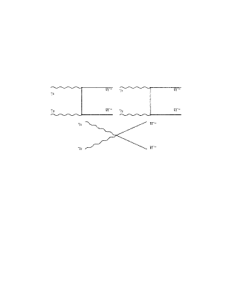
Figure 7: The Feynman diagrams for $W^{+}W^{-}$-production

We start from the explicit expression for the amplitude of the process $\gamma\gamma\rightarrow W^{+}W^{-}$

$$M=G_{\nu}\varepsilon_{\mu}(k_{1})\varepsilon_{\nu}(k_{2})\varepsilon_{\alpha}(p_{+})\varepsilon_{\beta}(p_{-})M_{T}^{\mu\nu\alpha\beta},$$ (44)

where

$$M_{T}^{\mu\nu\alpha\beta}=\sum_{i=1}^{3}M_{i}^{\mu\nu\alpha\beta},$$ (45)

$k_{1}$, $k_{2}$, $p_{+}$, $p_{-}$ are four-momenta for the $\gamma$, $\gamma$, $W^{+}$, $W^{-}$ and $\varepsilon_{\mu}(k_{1})$, $\varepsilon_{\nu}(k_{2})$, $\varepsilon_{\alpha}(p_{+})$, $\varepsilon_{\beta}(p_{-})$ their polarizations respectively,

$$G_{\nu}=e^{3}\cot\theta_{W}.$$

Total cross section of $\gamma\gamma$-boson production can be presented as

$$\sigma=\frac{1}{2s}\sum_{\lambda_{1}\lambda_{2}\lambda_{3}\lambda_{4}}{\int{|M_{\lambda_{1}\lambda_{2}\lambda_{3}\lambda_{4}}|^{2}d\Gamma}},$$ (46)

where $M_{\lambda_{1}\lambda_{2}\lambda_{3}\lambda_{4}}$ have been defined by eq. (45), $d\Gamma$ is phase space element of the bosons. The dependence of total cross section $\sigma(W^{+}W^{-})$ on anomalous parameters was investigated at the following experimental conditions:
– The center-of-mass energy of $\gamma\gamma(\sqrt{s})$ in $\gamma\gamma\rightarrow W^{+}W^{-}$ is fixed at 1 TeV;
– Photon luminosity $L$ is supposed to be 100 $\text{fb}^{-1}$/year;
– In ILC experiments for $\gamma\gamma$-scattering polarization states of the photon beams will be fixed by $J=0$ or $J=2$ states; – In addition it is assumed that the final $W$-bosons will be detected with certain polarization states;
and the results are presented in Figs. 8–13.

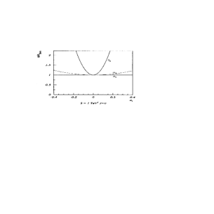
Figure 8: Dependencies of the ratio $\sigma/\sigma_{SM}$ on the various couplings

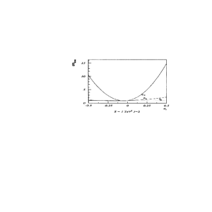
Figure 9: Dependencies of the ratio $\sigma/\sigma_{SM}$ on the various couplings

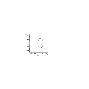
Figure 10: Contour plots on $(a_{c},\tilde{a}_{0})$ for $1\delta$ at $J=0$ photon beams

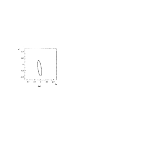
Figure 11: Contour plots on $(a_{0},a_{c})$ for $1\delta$ at $J=2$ photon beams

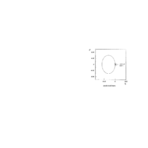
Figure 12: Contour plots on $(a_{0},\tilde{a}_{0})$ for $1\delta$

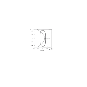
Figure 13: Contour plots on $(a_{0},\tilde{a}_{0})$ for $1\delta$

It is evident that minima of the curves are close to the Standard Model point $a_{i}=0$ since the interference between anomalous and standard part of cross section is very small. Through the region of $a_{i}$ is small (about 0.05) the cross section with anomalous constants may reach values of $1.6\sigma$. Taking into account a luminosity of photons and beams energy statistical error will be equal to 0.05 %. Therefore for precision analysis of experimental data it is important to calculate radiative corrections. We calculate $\mathcal{O}(\alpha)$ radiative correction giving maximal contribution to cross section value. It includes real photon emission as well as a set of one-loop diagrams (see. Fig. 14–15). Since of ILC-beams energy exceeds the threshold of three boson production this process must be considered as radiative effect too:

$$\begin{gathered}d\sigma(\gamma\gamma\rightarrow W^{+}W^{-})=\\ d\sigma^{\text{Born}}(\gamma\gamma\rightarrow W^{+}W^{-})+\end{gathered}$$

$$\begin{gathered}+\frac{1}{s}\Re(M^{\text{Born}}M^{1-\text{loop*}})d\Gamma^{(2)}+\\ +d\sigma^{\text{soft}}(\gamma\gamma\rightarrow W^{+}W^{-}\gamma)+\\ +d\sigma^{\text{hard}}(\gamma\gamma\rightarrow W^{+}W^{-}\gamma)+\\ +d\sigma^{Z}(\gamma\gamma\rightarrow W^{+}W^{-}Z).\end{gathered}$$ (47)

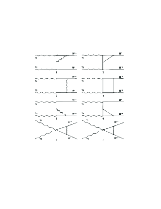
Figure 14: The Feynman diagrams of one-loop amplitudes of the $\gamma\gamma\rightarrow W^{+}W^{-}$

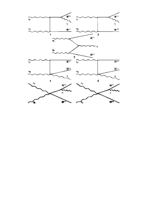
Figure 15: The Feynman diagrams of $\gamma\gamma\rightarrow W^{+}W^{-}$ accompanied real photon emission

Here $d\sigma^{\text{soft}}(\gamma\gamma\rightarrow W^{+}W^{-}\gamma)=d\sigma^{\text{Born}}(\gamma\gamma\rightarrow W^{+}W^{-})R^{\text{soft}}(\omega)$, where $\omega$ is soft photon energy cutoff,

$$\begin{gathered}R^{\text{soft}}=\frac{2\alpha}{\pi}\left\{\left[-1+\frac{1}{\beta}\left(1-\frac{2m_{W}^{2}}{s}\right)\ln{\frac{1+\beta}{1-\beta}}\right]\right.\times\\ \times\left.\left[\ln{2\omega}+\frac{1}{n-4}-\ln(2\sqrt{\pi}+\frac{C}{2})\right]+\right.\\ \left.+\frac{1}{2\beta}\ln{\frac{1+\beta}{1-\beta}}+\frac{1}{2\beta}\left(1-\frac{2m_{W}^{2}}{s}\right)\left(\mathop{Spence}{\frac{-2\beta}{1-\beta}}-\right.\right.\\ \left.\left.-\mathop{Spence}{\frac{2\beta}{1-\beta}}\right)\right\},\\ \beta=\sqrt{1-4m_{W}^{2}/s}.\end{gathered}$$ (48)

The differential cross section of hard photon emission is given by

$$\begin{gathered}d\sigma^{\text{hard}}(\gamma\gamma\rightarrow W^{+}W^{-}\gamma)=\\ d\sigma(\gamma\gamma\rightarrow W^{+}W^{-}\gamma)-\\ -d\sigma^{\text{soft}}(\gamma\gamma\rightarrow W^{+}W^{-}\gamma)\end{gathered}$$ (49)

and can not be factorized. $d\sigma^{\text{soft}}$ and $d\sigma^{\text{hard}}$ are independent from infrared divergence and from cutoff parameter.

Figure 16: Contour plots on $(a_{0},a_{c})$ for $+2\delta$ deviations of $\sigma(W^{+}W^{-})$

Fig. 16 demonstrates the considered radiative correction has significant magnitude and its calculation increases the precision of anomalous couplings measurement.

It must be noted that consideration of $W^{+}W^{-}\gamma$, $ZZ\gamma$, $Z\gamma\gamma$ processes in electron-positron annihilation gives additional information about $a_{0}$ and $a_{e}$, but the precision is two orders worse [18]. But $e^{+}e^{-}$ beams open possibility to measure four-boson connections [18]–[20] such as $W^{+}W^{-}$$W^{+}W^{-}$-, $W^{+}W^{-}ZZ$-, $ZZZZ$-production that it’s impossible for $\gamma\gamma$-physics. Corresponding four-boson anomalous weak interaction are presented by the Lagrangian with two four-dimension operators:

$$\begin{gathered}L_{Q}^{(a)}=\frac{1}{4}g_{w}^{2}\left[g_{o}\left(\vec{W}_{\mu}\cdot\vec{W}^{\mu}\right)^{2}+\right.\\ \left.+g_{c}\left(\vec{W}_{\mu}\cdot\vec{W}^{\nu}\right)\left(\vec{W}^{\mu}\cdot\vec{W}_{\nu}\right)\right].\end{gathered}$$ (50)

Here the first operator describes the exchange of neutral scalar particle with very high mass, but the second one corresponds to triplet of massive scalar particles. If four neutral boson vertex $(ZZZZ)$ is absent (e.g. $g_{0}=g_{c}$), interaction can be realized by massive vector boson exchange.

Using $e\gamma$ modes of two-boson production, $W^{+}W^{-}e$, $Z\gamma e$, $ZZe$, $W^{-}\gamma\nu$, $W^{-}Z\nu$, one can consider additional four-boson vertex $WWZ\gamma$ [21]:

$$\begin{gathered}L_{n}^{(6)}=i\frac{\pi\alpha}{m_{V}^{2}}a_{n}\vec{W}_{\alpha}\left(\vec{W}_{\nu}\cdot\vec{W}_{\mu}^{\alpha}\right)\vec{F}^{\mu\nu}.\end{gathered}$$ (51)

This Lagrangian conserves $U(1)_{EM}$, $C$-, $P$- and $SU(2)_{C}$-symmetry, but violates $SU(2)_{L}\otimes U(1)_{Y}$ symmetry.

From all above mentioned processes the most sensitive reactions for $a_{0}$ and $a_{e}$ investigation are $ZZe$ and $WWe$-production. The bounds of these constants magnitudes are one order better than in $e^{+}e^{-}$-process, but about 5 times worse than in $\gamma\gamma$-mode. The vertices $\gamma\gamma\gamma Z$ and $4\gamma$ are absent on tree level. One-loop contribution contain both fermion loops and $W$-boson loops. The last ones give contribution to be measured on photon collider [22].

6 Conclusion

We have analyzed the possible usage of $\gamma\gamma\to f\bar{f}\gamma$ reaction for the luminosity measurement at $J\!=\!0$ beams on linear photon collider. The achievable precision of the luminosity measuring is considered and calculated. The optimal conditions for that measurement are found (for the high magnitude of $J\!=\!0$ cross section and small $J\!=\!2$ background). The first-order QED correction to $\gamma\gamma\to l\bar{l}$ cross section is calculated and analyzed at $J\!=\!2$-beams.

The considered process gives the excellent opportunity for luminosity measurements with substantial accuracy.

The investigation of the sensitivity of process of $\gamma\gamma\to W^{+}W^{-}$ and $\gamma\gamma\to W^{+}W^{-}Z$ to genuine anomalous quartic couplings $a_{0}$, $a_{c}$ and $\tilde{a}_{0}$ was performed at center-of-mass energy $\sqrt{s}=1\,TeV$. It was discovered that two-boson production has great sensitivity to anomalous constants $a_{c}$ and $a_{0}$ but process $\gamma\gamma\to W^{+}W^{-}Z$ is more suitable for study of $\tilde{a}_{0}$.

The fact that the minimum of the curves are close to the SM point $a_{i}=0$ demonstrates the small value of the anomalous and the standard part interference. The first-order radiative correction to cross section $\sigma(\gamma\gamma\to W^{+}W^{-})$ has significant magnitude and its calculation increases the precision of the $a_{0}$ and $a_{c}$ measurement.

The theoretical analysis demonstrates that investigation of four-boson anomalous weak interaction in frame of four-dimension anomalous Lagrangian of $\gamma\gamma$ scattering as well as in frame of $e\gamma$ modes of two-boson production have great importance for reconstruction gauge group of electroweak interaction beyond the Standard theory of electroweak interaction.

References

• [1] I.F. Ginzburg, G.L. Kotkin, V.G. Serbo and V.I. Telnov, Nucl. Instr. Meth. 205, 47 (1983); I.F. Ginzburg, G.L. Kotkin, S.L. Panfil, V.G. Serbo and V.I. Telnov, Nucl. Instr. Meth. 219, 5 (1984).
• [2] E.A. Kuraev, M.V. Galynskii, M.I. Levchuk, Phys. Part. Nucl. 31, 76 (2000), Fiz. Elem. Chast. Atom. Yadra 31, 155 (2000); V. Telnov, Nucl. Instr. Meth. A494, 35 (2002), hep-ex/0207093.
• [3] T.V. Shishkina and V.V. Makarenko, hep-ph/0212409; V. Makarenko, K. Mönig, T. Shishkina, Eur. Phys. J. C30, d01, 011 (2003), LC-PHSM-2003-016, hep-ph/0306135; V.V. Makarenko and T.V. Shishkina, hep-ph/0310104.
• [4] V.V. Makarenko and T.V. Shishkina, Proceedings of 8th International School-Seminar On The Actual Problems Of Microwold Physics, Gomel (2003).
• [5] A. Denner and S. Dittmaier, Eur. Phys. J. C9, 425 (1999), hep-ph/9812411.
• [6] M. Moretti, Nucl. Phys. B484, 3 (1997), hep-ph/9604303; M. Moretti, hep-ph/9606225.
• [7] C. Carimalo, W.da Silva, F. Kapusta, Nucl. Phys. Proc. Suppl. 82, 391 (2000), hep-ph/9909339.
• [8] T. Shishkina and I. Sotsky, hep-ph/0312208.
• [9] P.de Causmaecker et al., Nucl. Phys. B206, 53 (1982); F.A. Berends et al., Nucl. Phys. B206, 61 (1982).
• [10] D.Yu. Bardin and N.M. Shumeiko, Nucl. Phys. B127, 242 (1977).
• [11] T.V. Kukhto(Shishkina), N.M. Shumeiko, S.I. Timoshin, J. Phys. G: Nucl. Phys. 13, 725 (1987).
• [12] S. Weinzierl, NIKHEF-00-012, hep-ph/0006269.
• [13] D.L. Borden and D.A. Bauer, D.O. Caldwell, Phys. Rev. D48, 4018 (1993); J.F. Gunion and H.E. Haber, Phys. Rev. D48, 5109 (1993).
• [14] K. Hagiwara et al., Nucl. Phys. B282, 253, (1987).
• [15] G. Belander et al., Eur. Phys. J. C283, 376 (2006); hep-ph/9908254.
• [16] I. Marfin and T. Shishkina, Nonlin. Phen. in Compl. Syst. 8, 4 150 (2005); Elem. Part. and Field 69, 4 710 (2006).
• [17] A. Denner et al., Eur. Phys. J. C20, 201 (2001); hep-ph/0104057.
• [18] G. Belander and F. Boundjema, Phys. Lett. B288, 201 (1992).
• [19] V. Barger, T. Han, R.J.N. Phillips, Phys. Rev. D39, 146 (1989).
• [20] C. Grosse-Knetter and D. Schidknecht, Phys. Lett. B302, 309 (1993).
• [21] O.J.P. Eboli, H.C. Gonzalez-Garcia, S.F. Novaes, Nucl. Phys. B411, 381 (1994).
• [22] G. Jikia and A. Thahbladze, Phys. Lett. B332, 441 (1994); Phys. Lett. B323, 453 (1994).