Global Solutions of Shock Reflection by Large-Angle Wedges for Potential Flow

Abstract

When a plane shock hits a wedge head on, it experiences a reflection-diffraction process and then a self-similar reflected shock moves outward as the original shock moves forward in time. Experimental, computational, and asymptotic analysis has shown that various patterns of shock reflection may occur, including regular and Mach reflection. However, most of the fundamental issues for shock reflection have not been understood, including the global structure, stability, and transition of the different patterns of shock reflection. Therefore, it is essential to establish the global existence and structural stability of solutions of shock reflection in order to understand fully the phenomena of shock reflection. On the other hand, there has been no rigorous mathematical result on the global existence and structural stability of shock reflection, including the case of potential flow which is widely used in aerodynamics. Such problems involve several challenging difficulties in the analysis of nonlinear partial differential equations such as mixed equations of elliptic-hyperbolic type, free boundary problems, and corner singularity where an elliptic degenerate curve meets a free boundary. In this paper we develop a rigorous mathematical approach to overcome these difficulties involved and establish a global theory of existence and stability for shock reflection by large-angle wedges for potential flow. The techniques and ideas developed here will be useful for other nonlinear problems involving similar difficulties.

1 02006 Gui-Qiang ChenMikhail Feldman Gui-Qiang Chen
Department of Mathematics, Northwestern University, Evanston, IL 60208-2730, USA;
School of Mathematical Sciences, Fudan University, Shanghai 200433, PRC;
Mikhail Feldman
Department of Mathematics, University of Wisconsin, Madison, WI 53706-1388, USA;

1 Introduction

We are concerned with the problems of shock reflection by wedges. These problems arise not only in many important physical situations but also are fundamental in the mathematical theory of multidimensional conservation laws since their solutions are building blocks and asymptotic attractors of general solutions to the multidimensional Euler equations for compressible fluids (cf. Courant-Friedrichs [16], von Neumann [49], and Glimm-Majda [22]; also see [4, 9, 21, 30, 44, 45, 48]). When a plane shock hits a wedge head on, it experiences a reflection-diffraction process and then a self-similar reflected shock moves outward as the original shock moves forward in time. The complexity of reflection picture was first reported by Ernst Mach [41] in 1878, and experimental, computational, and asymptotic analysis has shown that various patterns of shock reflection may occur, including regular and Mach reflection (cf. [4, 19, 22, 25, 26, 27, 44, 48, 49]). However, most of the fundamental issues for shock reflection have not been understood, including the global structure, stability, and transition of the different patterns of shock reflection. Therefore, it is essential to establish the global existence and structural stability of solutions of shock reflection in order to understand fully the phenomena of shock reflection. On the other hand, there has been no rigorous mathematical result on the global existence and structural stability of shock reflection, including the case of potential flow which is widely used in aerodynamics (cf. [5, 15, 22, 42, 44]). One of the main reasons is that the problems involve several challenging difficulties in the analysis of nonlinear partial differential equations such as mixed equations of elliptic-hyperbolic type, free boundary problems, and corner singularity where an elliptic degenerate curve meets a free boundary. In this paper we develop a rigorous mathematical approach to overcome these difficulties involved and establish a global theory of existence and stability for shock reflection by large-angle wedges for potential flow. The techniques and ideas developed here will be useful for other nonlinear problems involving similar difficulties.

The Euler equations for potential flow consist of the conservation law of mass and the Bernoulli law for the density $\rho$ and velocity potential $\Phi$:

(1.1) $$\partial_{t}\rho+\mbox{div}_{\bf x}(\rho\nabla_{\bf x}\Phi)=0,$$

(1.2) $$\partial_{t}\Phi+\frac{1}{2}|\nabla_{\bf x}\Phi|^{2}+i(\rho)=K,$$

where $K$ is the Bernoulli constant determined by the incoming flow and/or boundary conditions, and

$$i^{\prime}(\rho)=p^{\prime}(\rho)/\rho=c^{2}(\rho)/\rho$$

with $c(\rho)$ being the sound speed. For polytropic gas,

$$p(\rho)=\kappa\rho^{\gamma},\qquad c^{2}(\rho)=\kappa\gamma\rho^{\gamma-1},\qquad\gamma>1,\,\,\kappa>0.$$

Without loss of generality, we choose $\kappa=(\gamma-1)/\gamma$ so that

$$i(\rho)=\rho^{\gamma-1},\qquad c(\rho)^{2}=(\gamma-1)\rho^{\gamma-1},$$

which can be achieved by the following scaling:

$$({\bf x},t,K)\to(\alpha{\bf x},\alpha^{2}t,\alpha^{-2}K),\quad\alpha^{2}=\kappa\gamma/(\gamma-1).$$

Equations (1.1)–(1.2) can written as the following nonlinear equation of second order:

(1.3) $$\partial_{t}\hat{\rho}\big{(}K-\partial_{t}\Phi-\frac{1}{2}|\nabla_{\bf x}\Phi|^{2}\big{)}+\mbox{div}_{\bf x}\big{(}\hat{\rho}(K-\partial_{t}\Phi-\frac{1}{2}|\nabla_{\bf x}\Phi|^{2})\nabla_{\bf x}\Phi\big{)}=0,$$

where $\hat{\rho}(s)=s^{1/(\gamma-1)}=i^{-1}(s)$ for $s\geq 0$.

When a plane shock in the $({\bf x},t)$–coordinates, ${\bf x}=(x_{1},x_{2})\in{\bf R}^{2}$, with left state $(\rho,\nabla_{\bf x}\Psi)=(\rho_{1},u_{1},0)$ and right state $(\rho_{0},0,0),u_{1}>0,\rho_{0}<\rho_{1}$, hits a symmetric wedge

$$W:=\{|x_{2}|<x_{1}\tan\theta_{w},x_{1}>0\}$$

head on, it experiences a reflection-diffraction process, and the reflection problem can be formulated as the following mathematical problem.

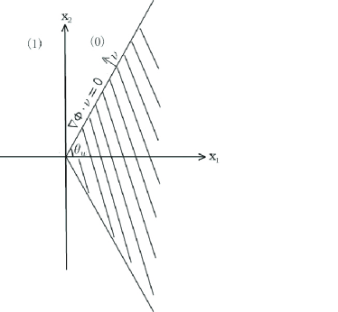
Problem 1 (Initial-Boundary Value Problem). Seek a solution of system (1.1)–(1.2) with $K=\rho_{0}^{\gamma-1}$, the initial condition at $t=0$:

(1.4) $$(\rho,\Phi)|_{t=0}=\begin{cases}(\rho_{0},0)\qquad&\mbox{for}\,\,|x_{2}|>x_{1}\tan\theta_{w},x_{1}>0,\\ (\rho_{1},u_{1}x_{1})\qquad&\mbox{for}\,\,x_{1}<0,\end{cases}$$

and the slip boundary condition along the wedge boundary $\partial W$:

(1.5) $$\nabla\Phi\cdot\nu|_{\partial W}=0,$$

where $\nu$ is the exterior unit normal to $\partial W$ (see Fig. 1).

Figure 1: Initial-boundary value problem

Notice that the initial-boundary value problem (1.1)–(1.5) is invariant under the self-similar scaling:

$$({\bf x},t)\to(\alpha{\bf x},\alpha t),\quad(\rho,\Phi)\to(\rho,\Phi/\alpha)\qquad\quad\mbox{for}\quad\alpha\neq 0.$$

Thus, we seek self-similar solutions with the form

$$\rho({\bf x},t)=\rho(\xi,\eta),\quad\Phi({\bf x},t)=t\,\psi(\xi,\eta)\qquad\quad\mbox{for}\quad(\xi,\eta)={\bf x}/t.$$

Then the pseudo-potential function $\varphi=\psi-\frac{1}{2}(\xi^{2}+\eta^{2})$ satisfies the following Euler equations for self-similar solutions:

(1.6) $$\mbox{div}\,(\rho\,D\varphi)+2\rho=0,$$

(1.7) $$\frac{1}{2}|D\varphi|^{2}+\varphi+\rho^{\gamma-1}=\rho_{0}^{\gamma-1},$$

where the divergence div and gradient $D$ are with respect to the self-similar variables $(\xi,\eta)$. This implies that the pseudo-potential function $\varphi(\xi,\eta)$ is governed by the following potential flow equation of second order:

(1.8) $$\mbox{div}\,\big{(}\rho(|D\varphi|^{2},\varphi)D\varphi\big{)}+2\rho(|D\varphi|^{2},\varphi)=0$$

with

(1.9) $$\rho(|D\varphi|^{2},\varphi)=\hat{\rho}(\rho_{0}^{\gamma-1}-\varphi-\frac{1}{2}|D\varphi|^{2}).$$

Then we have

(1.10) $$c^{2}=c^{2}(|D\varphi|^{2},\varphi,\rho_{0}^{\gamma-1})=(\gamma-1)(\rho_{0}^{\gamma-1}-\frac{1}{2}|D\varphi|^{2}-\varphi).$$

Equation (1.8) is a mixed equation of elliptic-hyperbolic type. It is elliptic if and only if

(1.11) $$|D\varphi|<c(|D\varphi|^{2},\varphi,\rho_{0}^{\gamma-1}),$$

which is equivalent to

(1.12) $$|D\varphi|<c_{*}(\varphi,\rho_{0},\gamma):=\sqrt{\frac{2(\gamma-1)}{\gamma+1}(\rho_{0}^{\gamma-1}-\varphi)}.$$

Shocks are discontinuities in the pseudo-velocity $D\varphi$. That is, if $\Omega^{+}$ and $\Omega^{-}:=\Omega\setminus\overline{\Omega^{+}}$ are two nonempty open subsets of $\Omega\subset{\bf R}^{2}$ and $S:=\partial\Omega^{+}\cap\Omega$ is a $C^{1}$ curve where $D\varphi$ has a jump, then $\varphi\in W^{1,1}_{loc}(\Omega)\cap C^{1}(\Omega^{\pm}\cup S)\cap C^{2}(\Omega^{\pm})$ is a global weak solution of (1.8) in $\Omega$ if and only if $\varphi$ is in $W^{1,\infty}_{loc}(\Omega)$ and satisfies equation (1.8) in $\Omega^{\pm}$ and the Rankine-Hugoniot condition on $S$:

(1.13) $$\left[\rho(|D\varphi|^{2},\varphi)D\varphi\cdot\nu\right]_{S}=0.$$

The continuity of $\varphi$ is followed by the continuity of the tangential derivative of $\varphi$ across $S$, which is a direct corollary of irrotationality of the pseudo-velocity. The discontinuity $S$ of $D\varphi$ is called a shock if $\varphi$ further satisfies the physical entropy condition that the corresponding density function $\rho(|D\varphi|^{2},\varphi)$ increases across $S$ in the pseudo-flow direction. We remark that the Rankine-Hugoniot condition (1.13) with the continuity of $\varphi$ across a shock for (1.8) is also fairly good approximation to the corresponding Rankine-Hugoniot conditions for the full Euler equations for shocks of small strength, since the errors are third-order in strength of the shock.

The plane incident shock solution in the $({\bf x},t)$–coordinates with states $(\rho,\nabla_{\bf x}\Psi)=(\rho_{0},0,0)$ and $(\rho_{1},u_{1},0)$ corresponds to a continuous weak solution $\varphi$ of (1.8) in the self-similar coordinates $(\xi,\eta)$ with the following form:

(1.14) $$\varphi_{0}(\xi,\eta)=-\frac{1}{2}(\xi^{2}+\eta^{2})\qquad\hbox{for }\,\,\xi>\xi_{0},$$

(1.15) $$\varphi_{1}(\xi,\eta)=-\frac{1}{2}(\xi^{2}+\eta^{2})+u_{1}(\xi-\xi_{0})\qquad\hbox{for }\,\,\xi<\xi_{0},$$

respectively, where

(1.16) $$\xi_{0}=\rho_{1}\sqrt{\frac{2(\rho_{1}^{\gamma-1}-\rho_{0}^{\gamma-1})}{\rho_{1}^{2}-\rho_{0}^{2}}}=\frac{\rho_{1}u_{1}}{\rho_{1}-\rho_{0}}>0$$

is the location of the incident shock, uniquely determined by $(\rho_{0},\rho_{1},\gamma)$ through (1.13). Since the problem is symmetric with respect to the axis $\eta=0$, it suffices to consider the problem in the half-plane $\eta>0$ outside the half-wedge

$$\Lambda:=\{\xi\leq 0,\eta>0\}\cup\{\eta>\xi\tan\theta_{w},\,\xi>0\}.$$

Then the initial-boundary value problem (1.1)–(1.5) in the $({\bf x},t)$–coordinates can be formulated as the following boundary value problem in the self-similar coordinates $(\xi,\eta)$.

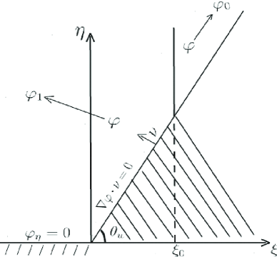
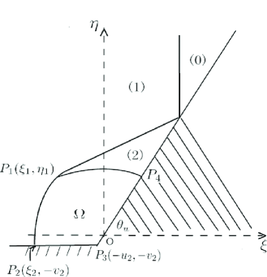
Problem 2 (Boundary Value Problem) (see Fig. 2). Seek a solution $\varphi$ of equation (1.8) in the self-similar domain $\Lambda$ with the slip boundary condition on the wedge boundary $\partial\Lambda$:

(1.17) $$D\varphi\cdot\nu|_{\partial\Lambda}=0$$

and the asymptotic boundary condition at infinity:

(1.18) $$\varphi\to\bar{\varphi}=\begin{cases}\varphi_{0}\qquad\mbox{for}\,\,\,\xi>\xi_{0},\eta>\xi\tan\theta_{w},\\ \varphi_{1}\qquad\mbox{for}\,\,\,\xi<\xi_{0},\eta>0,\end{cases}\qquad\mbox{when $\xi^{2}+\eta^{2}\to\infty$},$$

where (1.18) holds in the sense that $\displaystyle\lim_{R\to\infty}\|\varphi-\overline{\varphi}\|_{C(\Lambda\setminus B_{R}(0))}=0.$

Figure 2: Boundary value problem in the unbounded domain

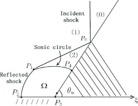
Since $\varphi_{1}$ does not satisfy the slip boundary condition (1.17), the solution must differ from $\varphi_{1}$ in $\{\xi<\xi_{0}\}\cap\Lambda$, thus a shock diffraction by the wedge occurs. In this paper, we first follow the von Neumann criterion to establish a local existence theory of regular shock reflection near the reflection point and show that the structure of solution is as in Fig. 3, when the wedge angle is large and close to $\pi/2$, in which the vertical line is the incident shock $S=\{\xi=\xi_{0}\}$ that hits the wedge at the point $P_{0}=(\xi_{0},\xi_{0}\tan\theta_{w})$, and state (0) and state (1) ahead of and behind $S$ are given by $\varphi_{0}$ and $\varphi_{1}$ defined in (1.14) and (1.15), respectively. The solutions $\varphi$ and $\varphi_{1}$ differ only in the domain $P_{0}{P_{1}}{P_{2}}{P_{3}}$ because of shock diffraction by the wedge vertex, where the curve $P_{0}{P_{1}}{P_{2}}$ is the reflected shock with the straight segment $P_{0}{P_{1}}$. State (2) behind $P_{0}{P_{1}}$ can be computed explicitly with the form:

(1.19) $$\varphi_{2}(\xi,\eta)=-\frac{1}{2}(\xi^{2}+\eta^{2})+u_{2}(\xi-\xi_{0})+(\eta-\xi_{0}\tan\theta_{w})u_{2}\tan\theta_{w},$$

which satisfies

$$D\varphi\cdot\nu=0\qquad\hbox{on }\,\partial\Lambda\cap\{\xi>0\};$$

the constant velocity $u_{2}$ and the angle $\theta_{s}$ between $P_{0}{P_{1}}$ and the $\xi$–axis are determined by $(\theta_{w},\rho_{0},\rho_{1},\gamma)$ from the two algebraic equations expressing (1.13) and continuous matching of state (1) and state (2) across $P_{0}{P_{1}}$, whose existence is exactly guaranteed by the condition on $(\theta_{w},\rho_{0},\rho_{1},\gamma)$ under which regular shock reflection is expected to occur.

Figure 3: Regular reflection

We develop a rigorous mathematical approach to extend the local theory to a global theory for solutions of regular shock reflection, which converge to the unique solution of the normal shock reflection when $\theta_{w}$ tends to $\pi/2$. The solution $\varphi$ is pseudo-subsonic within the sonic circle for state (2) with center $(u_{2},u_{2}\tan\theta_{w})$ and radius $c_{2}>0$ (the sonic speed) and is pseudo-supersonic outside this circle containing the arc ${P_{1}}{P_{4}}$ in Fig. 3, so that $\varphi_{2}$ is the unique solution in the domain $P_{0}{P_{1}}{P_{4}}$, as argued in [9, 45]. In the domain $\Omega$, the solution is expected to be pseudo-subsonic, smooth, and $C^{1}$-smoothly matching with state (2) across ${P_{1}}{P_{4}}$ and to satisfy $\varphi_{\eta}=0$ on ${P_{2}}{P_{3}}$; the transonic shock curve ${P_{1}}{P_{2}}$ matches up to second-order with $P_{0}{P_{1}}$ and is orthogonal to the $\xi$-axis at the point ${P_{2}}$ so that the standard reflection about the $\xi$–axis yields a global solution in the whole plane. Then the solution of Problem 2 can be shown to be the solution of Problem 1.

Main Theorem. There exist $\theta_{c}=\theta_{c}(\rho_{0},\rho_{1},\gamma)\in(0,\pi/2)$ and $\alpha=\alpha(\rho_{0},\rho_{1},\gamma)\in(0,1/2)$ such that, when $\theta_{w}\in[\theta_{c},\pi/2)$, there exists a global self-similar solution

$$\Phi({\bf x},t)=t\,\varphi(\frac{\bf x}{t})+\frac{|\bf x|^{2}}{2t}\qquad\mbox{for}\,\,\frac{\bf x}{t}\in\Lambda,\,t>0$$

with

$$\rho({\bf x},t)=(\rho_{0}^{\gamma-1}-\Phi_{t}-\frac{1}{2}|\nabla_{\bf x}\Phi|^{2})^{\frac{1}{\gamma-1}}$$

of Problem 1 (equivalently, Problem 2) for shock reflection by the wedge, which satisfies that, for $(\xi,\eta)={\bf x}/t$,

$$\varphi\in C^{\infty}(\Omega)\cap C^{1,\alpha}(\bar{\Omega}),$$

(1.20) $$\varphi=\left\{\begin{array}[]{ll}\varphi_{0}\qquad\mbox{for}\,\,\xi>\xi_{0}\mbox{ and }\eta>\xi\tan\theta_{w},\\ \varphi_{1}\qquad\mbox{for}\,\,\xi<\xi_{0}\mbox{ and above the reflection shock}\,\,P_{0}{P_{1}}{P_{2}},\\ \varphi_{2}\qquad\mbox{in}\,\,P_{0}{P_{1}}{P_{4}},\end{array}\right.$$

$\varphi$ is $C^{1,1}$ across the part ${P_{1}}{P_{4}}$ of the sonic circle including the endpoints ${P_{1}}$ and ${P_{4}}$, and the reflected shock $P_{0}{P_{1}}{P_{2}}$ is $C^{2}$ at ${P_{1}}$ and $C^{\infty}$ except ${P_{1}}$. Moreover, the solution $\varphi$ is stable with respect to the wedge angle in $W^{1,1}_{loc}(\overline{\Lambda})$ and converges in $W^{1,1}_{loc}(\overline{\Lambda})$ to the solution of the normal reflection described in §3 as $\theta_{w}\to\pi/2$.

One of the main difficulties for the global existence is that the ellipticity condition (1.12) for (1.8) is hard to control, in comparison to our earlier work on steady flow [10, 11]. The second difficulty is that the ellipticity degenerates at the sonic circle ${P_{1}}{P_{4}}$ (the boundary of the pseudo-subsonic flow). The third difficulty is that, on ${P_{1}}{P_{4}}$, we need to match the solution in $\Omega$ with $\varphi_{2}$ at least in $C^{1}$, that is, the two conditions on the fixed boundary ${P_{1}}{P_{4}}$: the Dirichlet and conormal conditions, which are generically overdetermined for an elliptic equation since the conditions on the other parts of boundary have been prescribed. Thus we have to prove that, if $\varphi$ satisfies (1.8) in $\Omega$, the Dirichlet continuity condition on the sonic circle, and the appropriate conditions on the other parts of $\partial\Omega$ derived from Problem 2, then the normal derivative $D\varphi\cdot\nu$ automatically matches with $D\varphi_{2}\cdot\nu$ along ${P_{1}}{P_{4}}$. We show that, in fact, this follows from the structure of elliptic degeneracy of (1.8) on ${P_{1}}{P_{4}}$ for the solution $\varphi$. Indeed, equation (1.8), written in terms of the function $u=\varphi-\varphi_{2}$ in the $(x,y)$–coordinates defined near ${P_{1}}{P_{4}}$ such that ${P_{1}}{P_{4}}$ becomes a segment on $\{x=0\}$, has the form:

(1.21) $$\big{(}2x-(\gamma+1)u_{x}\big{)}u_{xx}+\frac{1}{c_{2}^{2}}u_{yy}-u_{x}=0\qquad\,\,\mbox{in }x>0\mbox{ and near }x=0,$$

plus the “small” terms that are controlled by $\pi/2-\theta_{w}$ in appropriate norms. Equation (1.21) is elliptic if $u_{x}<2x/(\gamma+1)$. Thus, we need to obtain the $C^{1,1}$ estimates near ${P_{1}}{P_{4}}$ to ensure $|u_{x}|<2x/(\gamma+1)$ which in turn implies both the ellipticity of the equation in $\Omega$ and the match of normal derivatives $D\varphi\cdot\nu=D\varphi_{2}\cdot\nu$ along ${P_{1}}{P_{4}}$. Taking into account the “small” terms to be added to equation (1.21), we need to make the stronger estimate $|u_{x}|\leq 4x/\big{(}3(\gamma+1)\big{)}$ and assume that $\pi/2-\theta_{w}$ is appropriately small to control these additional terms. Another issue is the non-variational structure and nonlinearity of this problem which makes it hard to apply directly the approaches of Caffarelli [6] and Alt-Caffarelli-Friedman [1, 2]. Moreover, the elliptic degeneracy and geometry of the problem makes it difficult to apply the hodograph transform approach in Kinderlehrer-Nirenberg [28] and Chen-Feldman [12] to fix the free boundary.

For these reasons, one of the new ingredients in our approach is to further develop the iteration scheme in [10, 11] to a partially modified equation. We modify equation (1.8) in $\Omega$ by a proper cutoff that depends on the distance to the sonic circle, so that the original and modified equations coincide for $\varphi$ satisfying $|u_{x}|\leq 4x/\big{(}3(\gamma+1)\big{)}$, and the modified equation ${\mathcal{N}}\varphi=0$ is elliptic in $\Omega$ with elliptic degeneracy on ${P_{1}}{P_{4}}$. Then we solve a free boundary problem for this modified equation: The free boundary is the curve ${P_{1}}{P_{2}}$, and the free boundary conditions on ${P_{1}}{P_{2}}$ are $\varphi=\varphi_{1}$ and the Rankine-Hugoniot condition (1.13).

On each step, an “iteration free boundary” curve ${P_{1}}{P_{2}}$ is given, and a solution of the modified equation ${\mathcal{N}}\varphi=0$ is constructed in $\Omega$ with the boundary condition (1.13) on ${P_{1}}{P_{2}}$, the Dirichlet condition $\varphi=\varphi_{2}$ on the degenerate circle ${P_{1}}{P_{4}}$, and $D\varphi\cdot\nu=0$ on ${P_{2}}{P_{3}}$ and ${P_{3}}{P_{4}}$. Then we prove that $\varphi$ is in fact $C^{1,1}$ up to the boundary ${P_{1}}{P_{4}}$, especially $|{D}(\varphi-\varphi_{2})|\leq Cx$, by using the nonlinear structure of elliptic degeneracy near ${P_{1}}{P_{4}}$ which is modeled by equation (1.21) and a scaling technique similar to Daskalopoulos-Hamilton [17] and Lin-Wang [40]. Furthermore, we modify the “iteration free boundary” curve ${P_{1}}{P_{2}}$ by using the Dirichlet condition $\varphi=\varphi_{1}$ on ${P_{1}}{P_{2}}$. A fixed point $\varphi$ of this iteration procedure is a solution of the free boundary problem for the modified equation. Moreover, we prove the precise gradient estimate: $|u_{x}|<4x/\big{(}3(\gamma+1)\big{)}$, which implies that $\varphi$ satisfies the original equation (1.8).

Some efforts have been made mathematically for the reflection problem via simplified models. One of these models, the unsteady transonic small-disturbance (UTSD) equation, was derived and used in Keller-Blank [27], Hunter-Keller [26], Hunter [25], Morawetz [44], and the references cited therein for asymptotic analysis of shock reflection. Also see Zheng [50] for the pressure gradient equation and Canic-Keyfitz-Kim [7] for the UTSD equation and the nonlinear wave system. On the other hand, in order to deal with the reflection problem, some asymptotic methods have been also developed. Lighthill [38, 39] studied shock reflection under the assumption that the wedge angle is either very small or close to $\pi/2$. Keller-Blank [27], Hunter-Keller [26], and Harabetian [24] considered the problem under the assumption that the shock is so weak that its motion can be approximated by an acoustic wave. For a weak incident shock and a wedge with small angle in the context of potential flow, by taking the jump of the incident shock as a small parameter, the nature of the shock reflection pattern was explored in Morawetz [44] by a number of different scalings, a study of mixed equations, and matching the asymptotics for the different scalings. Also see Chen [14] for a linear approximation of shock reflection when the wedge angle is close to $\pi/2$ and Serre [45] for an apriori analysis of solutions of shock reflection and related discussions in the context of the Euler equations for isentropic and adiabatic fluids.

The organization of this paper is the following. In §2, we present the potential flow equation in self-similar coordinates and exhibit some basic properties of solutions to the potential flow equation. In §3, we discuss the normal reflection solution and then follow the von Neumann criterion to derive the necessary condition for the existence of regular reflection and show that the shock reflection can be regular locally when the wedge angle is large. In §4, the shock reflection problem is reformulated and reduced to a free boundary problem for a second-order nonlinear equation of mixed type in a convenient form. In §5, we develop an iteration scheme, along with an elliptic cutoff technique, to solve the free boundary problem and set up the ten detailed steps of the iteration procedure.

Finally, we complete the remaining steps in our iteration procedure in §6–§9: Step 2 for the existence of solutions of the boundary value problem to the degenerate elliptic equation via the vanishing viscosity approximation in §6; Steps 3–8 for the existence of the iteration map and its fixed point in §7; and Step 9 for the removal of the ellipticity cutoff in the iteration scheme by using appropriate comparison functions and deriving careful global estimates for some directional derivatives of the solution in §8. We complete the proof of Main Theorem in §9. Careful estimates of the solutions to both the “almost tangential derivative” and oblique derivative boundary value problems for elliptic equations are made in Appendix, which are applied in §6–§7.

2 Self-Similar Solutions of the Potential Flow Equation

In this section we present the potential flow equation in self-similar coordinates and exhibit some basic properties of solutions of the potential flow equation (also see Morawetz [44]).

The potential flow equation for self-similar solutions Equation (1.8) is a mixed equation of elliptic-hyperbolic type. It is elliptic if and only if (1.12) holds. The hyperbolic-elliptic boundary is the pseudo-sonic curve: $|D\varphi|=c_{*}(\varphi,\rho_{0},\gamma)$.

We first define the notion of weak solutions of (1.8)–(1.9). Essentially, we require the equation to be satisfied in the distributional sense.

Definition 2.1 (Weak Solutions)

A function $\varphi\in W^{1,1}_{loc}(\Lambda)$ is called a weak solution of (1.8)–(1.9) in a self-similar domain $\Lambda$ if

1. $\rho_{0}^{\gamma-1}-\varphi-\frac{1}{2}|D\varphi|^{2}\geq 0$ a.e. in $\Lambda$;

2. $(\rho(|D\varphi|^{2},\varphi),\rho(|D\varphi|^{2},\varphi)|{D}\varphi|)\in(L^{1}_{loc}(\Lambda))^{2}$;

3. For every $\zeta\in C^{\infty}_{c}(\Lambda)$,

   $$\int_{\Lambda}\Big{(}\rho(|D\varphi|^{2},\varphi){D}\varphi\cdot{D}\zeta-2\rho(|D\varphi|^{2},\varphi)\zeta\Big{)}\,d{\xi}d{\eta}=0.$$

It is straightforward to verify the equivalence between time-dependent self-similar solutions and weak solutions of (1.8) defined in Definition 2.1 in the weak sense. It can also be verified that, if $\varphi\in C^{1,1}(\Lambda)$ (and thus $\varphi$ is twice differentiable a.e. in $\Lambda$), then $\varphi$ is a weak solution of (1.8) in $\Lambda$ if and only if $\varphi$ satisfies equation (1.8) a.e. in $\Lambda$. Finally, it is easy to see that, if $\Lambda^{+}$ and $\Lambda^{-}=\Lambda\setminus\overline{\Lambda^{+}}$ are two nonempty open subsets of $\Lambda\subset{\bf R}^{2}$ and $S=\partial\Lambda^{+}\cap\Lambda$ is a $C^{1}$ curve where $D\varphi$ has a jump, then $\varphi\in W^{1,1}_{loc}(D)\cap C^{1}(\Lambda^{\pm}\cup S)\cap C^{1,1}(\Lambda^{\pm})$ is a weak solution of (1.8) in $\Lambda$ if and only if $\varphi$ is in $W^{1,\infty}_{loc}(\Lambda)$ and satisfies equation (1.8) a.e. in $\Lambda^{\pm}$ and the Rankine-Hugoniot condition (1.13) on $S$.

Note that, for $\varphi\in C^{1}(\Lambda^{\pm}\cup S)$, the condition $\varphi\in W^{1,\infty}_{loc}(\Lambda)$ implies

(2.1) $$[\varphi]_{S}=0.$$

Furthermore, the Rankine-Hugoniot conditions imply

(2.2) $$[\varphi_{\xi}][\rho\varphi_{\xi}]-[\varphi_{\eta}][\rho\varphi_{\eta}]=0\qquad\text{on }S$$

which is a useful identity.

A discontinuity of ${D}\varphi$ satisfying the Rankine-Hugoniot conditions (2.1) and (1.13) is called a shock if it satisfies the physical entropy condition: The density function $\rho$ increases across a shock in the pseudo-flow direction. The entropy condition indicates that the normal derivative function $\varphi_{\nu}$ on a shock always decreases across the shock in the pseudo-flow direction.

The states with constant density When the density $\rho$ is constant, (1.8)–(1.9) imply that $\varphi$ satisfies

$$\Delta\varphi+2=0,\qquad\frac{1}{2}|D\varphi|^{2}+\varphi=const.$$

This implies $(\Delta\varphi)_{\xi}=0,(\Delta\varphi)_{\eta}=0,$ and $(\varphi_{\xi\xi}+1)^{2}+\varphi_{\xi\eta}^{2}=0$. Thus, we have

$$\varphi_{\xi\xi}=-1,\quad\varphi_{\xi\eta}=0,\quad\varphi_{\eta\eta}=-1,$$

which yields

(2.3) $$\varphi(\xi,\eta)=-\frac{1}{2}(\xi^{2}+\eta^{2})+a\xi+b\eta+c,$$

where $a,b$, and $c$ are constants.

Location of the incident shock Consider state $(0)$: $(\rho_{0},u_{0},v_{0})=(\rho_{0},0,0)$ with $\rho_{0}>0$ and state $(1)$: $(\rho_{1},u_{1},v_{1})$ $=(\rho_{1},u_{1},0)$ with $\rho_{1}>\rho_{0}>0$ and $u_{1}>0$. The plane incident shock solution with state (0) and state (1) corresponds to a continuous weak solution $\varphi$ of (1.8) in the self-similar coordinates $(\xi,\eta)$ with form (1.14) and (1.15) for state (0) and state (1) respectively, where $\xi=\xi_{0}>0$ is the location of the incident shock.

The unit normal to the shock line is $\nu=(1,0)$. Using (2.2), we have

$$u_{1}=\frac{\rho_{1}-\rho_{0}}{\rho_{1}}\xi_{0}>0.$$

Then (1.9) implies

$$\rho_{1}^{\gamma-1}-\rho_{0}^{\gamma-1}=-\frac{1}{2}|D\varphi_{1}|^{2}-\varphi_{1}=\frac{1}{2}\frac{\rho_{1}^{2}-\rho_{0}^{2}}{\rho_{1}^{2}}\xi_{0}^{2}.$$

Therefore, we have

(2.4) $$u_{1}=(\rho_{1}-\rho_{0})\sqrt{\frac{2(\rho_{1}^{\gamma-1}-\rho_{0}^{\gamma-1})}{\rho_{1}^{2}-\rho_{0}^{2}}},$$

and the location of the incident shock in the self-similar coordinates is $\xi=\xi_{0}>u_{1}$ determined by (1.16).

3 The von Neumann Criterion and Local Theory for Shock Reflection

In this section, we first discuss the normal reflection solution. Then we follow the von Neumann criterion to derive the necessary condition for the existence of regular reflection and show that the shock reflection can be regular locally when the wedge angle is large, that is, when $\theta_{w}$ is close to $\pi/2$ and, equivalently, the angle between the incident shock and the wedge

(3.1) $$\sigma:=\pi/2-\theta_{w}$$

tends to zero.

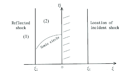
Normal shock reflection In this case, the wedge angle is $\pi/2$, i.e., $\sigma=0$, and the incident shock normally reflects (see Fig. 4). The reflected shock is also a plane at $\xi=\bar{\xi}<0$, which will be defined below. Then $\bar{u}_{2}=\bar{v}_{2}=0$, state (1) has form (1.15), and state (2) has the form:

(3.2) $$\varphi_{2}(\xi,\eta)=-\frac{1}{2}(\xi^{2}+\eta^{2})+u_{1}(\bar{\xi}-\xi_{0})\qquad\mbox{for}\,\,\xi\in(\bar{\xi},0),$$

where $\xi_{0}=\rho_{1}u_{1}/(\rho_{1}-\rho_{0})>0$ may be regarded to be the position of the incident shock.

Figure 4: Normal reflection

At the reflected shock $\xi=\bar{\xi}<0$, the Rankine-Hugoniot condition (2.2) implies

(3.3) $$\bar{\xi}=-\frac{\rho_{1}u_{1}}{\bar{\rho}_{2}-\rho_{1}}<0.$$

We use the Bernoulli law (1.7):

$$\rho_{0}^{\gamma-1}=\rho_{1}^{\gamma-1}+\frac{1}{2}u_{1}^{2}-u_{1}\xi_{0}=\bar{\rho}_{2}^{\gamma-1}+u_{1}(\bar{\xi}-\xi_{0})$$

to obtain

(3.4) $$\bar{\rho}_{2}^{\gamma-1}=\rho_{1}^{\gamma-1}+\frac{1}{2}u_{1}^{2}+\frac{\rho_{1}u_{1}^{2}}{\bar{\rho}_{2}-\rho_{1}}.$$

It can be shown that there is a unique solution $\bar{\rho}_{2}$ of (3.4) such that

$$\bar{\rho}_{2}>\rho_{1}.$$

Indeed, for fixed $\gamma>1$ and $\rho_{1},u_{1}>0$ and for $F(\bar{\rho}_{2})$ that is the right-hand side of (3.4), we have

$$\lim_{s\to\infty}F(s)=\rho_{1}^{\gamma-1}+\frac{1}{2}u_{1}^{2}>\rho_{1}^{\gamma-1},\quad\lim_{s\to\rho_{1}+}F(s)=\infty,$$

$$F^{\prime}(s)=-\frac{\rho_{1}u_{1}^{2}}{(s-\rho_{1})^{2}}<0\qquad\,\mbox{ for}\,\,s>\rho_{1}.$$

Thus there exists a unique $\bar{\rho}_{2}\in(\rho_{1},\infty)$ satisfying $\bar{\rho}_{2}^{\gamma-1}=F(\bar{\rho}_{2})$, i.e., (3.4). Then the position of the reflected shock $\xi=\bar{\xi}<0$ is uniquely determined by (3.3).

Moreover, for the sonic speed $\bar{c}_{2}=\sqrt{(\gamma-1)\bar{\rho}_{2}^{\gamma-1}}$ of state (2), we have

(3.5) $$|\bar{\xi}|<\bar{c}_{2}.$$

This can be seen as follows. First note that

(3.6) $$\bar{\rho}_{2}^{\gamma-1}-\rho_{1}^{\gamma-1}=\beta(\bar{\rho}_{2}-\rho_{1}),$$

where $\beta=(\gamma-1)\rho_{*}^{\gamma-2}>0$ for some $\rho_{*}\in(\rho_{1},\bar{\rho}_{2})$. We consider two cases, respectively.

Case 1. $\gamma\geq 2$. Then

(3.7) $$0<(\gamma-1)\rho_{1}^{\gamma-2}\leq\beta\leq(\gamma-1)\bar{\rho}_{2}^{\gamma-2}.$$

Since $\beta>0$ and $\bar{\rho}_{2}>\rho_{1}$, we use (3.4) and (3.6) to find

$$\bar{\rho}_{2}=\rho_{1}+\frac{u_{1}}{4\beta}\big{(}u_{1}+\sqrt{u_{1}^{2}+16\beta\rho_{1}}\big{)},$$

and hence

(3.8) $$\bar{\xi}=-\frac{4\beta\rho_{1}}{u_{1}+\sqrt{u_{1}^{2}+16\beta\rho_{1}}}.$$

Then using (3.7)–(3.8), $\bar{\rho}_{2}>\rho_{1}>0$, and $u_{1}>0$ yields

$$|\bar{\xi}|=\frac{4\beta\rho_{1}}{u_{1}+\sqrt{u_{1}^{2}+16\beta\rho_{1}}}<\sqrt{\beta\rho_{1}}\leq\sqrt{(\gamma-1)\bar{\rho}_{2}^{\gamma-2}\bar{\rho}_{2}}=\bar{c}_{2}.$$

Case 2. $1<\gamma<2$. Then, since $\bar{\rho}_{2}>\rho_{1}>0$,

(3.9) $$0<(\gamma-1)\bar{\rho}_{2}^{\gamma-2}\leq\beta\leq(\gamma-1)\rho_{1}^{\gamma-2}.$$

Since $\beta>0$, (3.8) holds by the calculation as in Case 1. Now we use (3.8)–(3.9), $\bar{\rho}_{2}>\rho_{1}>0$, $u_{1}>0$, and $1<\gamma<2$ to find again

$$|\bar{\xi}|<\sqrt{\beta\rho_{1}}\leq\sqrt{(\gamma-1)\rho_{1}^{\gamma-1}}\leq\sqrt{(\gamma-1)\bar{\rho}_{2}^{\gamma-1}}=\bar{c}_{2}.$$

This shows that (3.5) holds in general.

The von Neumann criterion and local theory for regular reflection In this subsection, we first follow the von Neumann criterion to derive the necessary condition for the existence of regular reflection and show that, when the wedge angle is large, there exists a unique state (2) with two-shock structure at the reflected point, which is close to the solution $(\bar{\rho}_{2},\bar{u}_{2},\bar{v}_{2})=(\bar{\rho}_{2},0,0)$ of normal reflection for which $\theta_{w}=\pi/2$ in §3.1.

For a possible two-shock configuration satisfying the corresponding boundary condition on the wedge $\eta=\xi\tan\theta_{w}$, the three state functions $\varphi_{j},j=0,1,2$, must be of form (1.14), (1.15), and (1.19) (cf. (2.3)).

Set the reflected point $P_{0}=(\xi_{0},\xi_{0}\tan\theta_{w})$ and assume that the line that coincides with the reflected shock in state (2) will intersect with the axis $\eta=0$ at the point $(\tilde{\xi},0)$ with the angle $\theta_{s}$ between the line and $\eta=0$.

Note that $\varphi_{1}(\xi,\eta)$ is defined by (1.15). The continuity of $\varphi$ at $(\tilde{\xi},0)$ yields

(3.10) $$\varphi_{2}(\xi,\eta)=-\frac{1}{2}(\xi^{2}+\eta^{2})+u_{2}\xi+v_{2}\eta+\big{(}u_{1}(\tilde{\xi}-\xi_{0})-u_{2}\tilde{\xi}\big{)}.$$

Furthermore, $\varphi_{2}$ must satisfy the slip boundary condition at $P_{0}$:

(3.11) $$v_{2}=u_{2}\tan\theta_{w}.$$

Also we have

(3.12) $$\tilde{\xi}=\xi_{0}-\xi_{0}\frac{\tan\theta_{w}}{\tan\theta_{s}}.$$

The Bernoulli law (1.7) becomes

(3.13) $$\rho_{0}^{\gamma-1}=\rho_{2}^{\gamma-1}+\frac{1}{2}(u_{2}^{2}+v_{2}^{2})+(u_{1}-u_{2})\tilde{\xi}-u_{1}\xi_{0}.$$

Moreover, the continuity of $\varphi$ on the shock implies that $D(\varphi_{2}-\varphi_{1})$ is orthogonal to the tangent direction of the reflected shock:

(3.14) $$(u_{2}-u_{1},v_{2})\cdot(\cos\theta_{s},\sin\theta_{s})=0,$$

that is,

(3.15) $$u_{2}=u_{1}\frac{\cos\theta_{w}\cos\theta_{s}}{\cos(\theta_{w}-\theta_{s})}.$$

The Rankine-Hugoniot condition (1.13) along the reflected shock is

$$[\rho\,D\varphi]\cdot(\sin\theta_{s},-\cos\theta_{s})=0,$$

that is,

(3.16) $$\rho_{1}(u_{1}-\tilde{\xi})\sin\theta_{s}=\rho_{2}\big{(}u_{2}\frac{\sin(\theta_{s}-\theta_{w})}{\cos\theta_{w}}-\tilde{\xi}\sin\theta_{s}\big{)}.$$

Combining (3.12)–(3.16), we obtain the following system for $(\rho_{2},\theta_{s},\tilde{\xi})$:

(3.17) $$(\tilde{\xi}-\xi_{0})\cos\theta_{w}+\xi_{0}\sin\theta_{w}\cot\theta_{s}=0,$$

(3.18) $$\rho_{2}^{\gamma-1}+\frac{u_{1}^{2}\cos^{2}\theta_{s}}{2\cos^{2}(\theta_{w}-\theta_{s})}+\frac{u_{1}\sin\theta_{w}\sin\theta_{s}}{\cos(\theta_{w}-\theta_{s})}\tilde{\xi}-u_{1}\xi_{0}-\rho_{0}^{\gamma-1}=0,$$

(3.19) $$\big{(}u_{1}\cos\theta_{s}\tan(\theta_{s}-\theta_{w})-\tilde{\xi}\sin\theta_{s}\big{)}\rho_{2}-\rho_{1}(u_{1}-\tilde{\xi})\sin\theta_{s}=0.$$

The condition for solvability of this system is the necessary condition for the existence of regular shock reflection.

Now we compute the Jacobian $J$ in terms of $(\rho_{2},\theta_{s},\tilde{\xi})$ at the normal reflection solution state $(\bar{\rho}_{2},\frac{\pi}{2},\bar{\xi})$ in §3.1 for state $(2)$ when $\theta_{w}=\pi/2$ to obtain

$$J=-\xi_{0}\big{(}(\gamma-1)\bar{\rho}_{2}^{\gamma-2}(\bar{\rho}_{2}-\rho_{1})-u_{1}\bar{\xi}\big{)}<0,$$

since $\bar{\rho}_{2}>\rho_{1}$ and $\bar{\xi}<0$. Then, by the Implicit Function Theorem, when $\theta_{w}$ is near $\pi/2$, there exists a unique solution $(\rho_{2},\theta_{s},\tilde{\xi})$ close to $(\bar{\rho}_{2},\frac{\pi}{2},\bar{\xi})$ of system (3.17)–(3.19). Moreover, $(\rho_{2},\theta_{s},\tilde{\xi})$ are smooth functions of $\sigma=\pi/2-\theta_{w}\in(0,\sigma_{1})$ for $\sigma_{1}>0$ depending only on $\rho_{0},\rho_{1}$, and $\gamma$. In particular,

(3.20) $$|\rho_{2}-\bar{\rho}_{2}|+|\pi/2-\theta_{s}|+|\tilde{\xi}-\bar{\xi}|+|c_{2}-\bar{c}_{2}|\leq C\sigma,$$

where $\displaystyle c_{2}=\sqrt{(\gamma-1)\rho_{2}^{\gamma-1}}$ is the sonic speed of state (2).

Reducing $\sigma_{1}>0$ if necessary, we find that, for any $\sigma\in(0,\sigma_{1})$,

(3.21) $$\tilde{\xi}<0$$

from (3.3) and (3.20). Since $\theta_{w}\in(\pi/2-\sigma_{1},\pi/2)$, then $\theta_{s}\in(\pi/4,3\pi/4)$ if $\sigma_{1}$ is small, which implies $\sin\theta_{s}>0$. We conclude from (3.17), (3.21), and $\xi_{0}>0$ that $\tan\theta_{w}>\tan\theta_{s}>0$. Thus,

(3.22) $$\pi/4<\theta_{s}<\theta_{w}<\pi/2.$$

Now, given $\theta_{w}$, we define $\varphi_{2}$ as follows: We have shown that there exists a unique solution $(\rho_{2},\theta_{s},\tilde{\xi})$ close to $(\bar{\rho}_{2},\frac{\pi}{2},\bar{\xi})$ of system (3.17)–(3.19). Define $u_{2}$ by (3.15), $v_{2}$ by (3.11), and $\varphi_{2}$ by (3.10). Then the shock connecting state (1) with state (2) is the straight line $S_{12}=\{({\xi},{\eta})\;:\,\varphi_{1}({\xi},{\eta})=\varphi_{2}({\xi},{\eta})\}$, which is $\xi={\eta}\cot\theta_{s}+\tilde{\xi}$ by (1.15), (3.10), and (3.15). Now (3.19) implies that the Rankine-Hugoniot condition (1.13) holds on $S_{12}$. Moreover, (3.11) and (3.15) imply (3.14). Thus the solution $(\theta_{s},\rho_{2},u_{2},v_{2})$ satisfies (3.11)–(3.19). Furthermore, (3.17) implies that the point $P_{0}$ lies on $S_{12}$, and (3.18) implies (3.13) that is the Bernoulli law:

(3.23) $$\rho_{2}^{\gamma-1}+{1\over 2}|{D}\varphi_{2}|^{2}+\varphi_{2}=\rho_{0}^{\gamma-1}.$$

Thus we have established the local existence of the two-shock configuration near the reflected point so that, behind the straight reflected shock emanating from the reflection point, state (2) is pseudo-supersonic up to the sonic circle of state (2). Furthermore, this local structure is stable in the limit $\theta_{w}\to\pi/2$, i.e., $\sigma\to 0$.

We also notice from (3.11) and (3.15) with the use of (3.20) and (3.22) that

(3.24) $$|u_{2}|+|v_{2}|\leq C\sigma.$$

Furthermore, from (3.5) and the continuity of $\rho_{2}$ and $\tilde{\xi}$ with respect to $\theta_{w}$ on $(\pi/2-\sigma_{1},\pi/2]$, it follows that, if $\sigma>0$ is small,

(3.25) $$|\tilde{\xi}|<c_{2}.$$

In §4–§9, we prove that this local theory for the existence of two shock configuration can be extended to a global theory for regular shock reflection.

4 Reformulation of the Shock Reflection Problem

We first assume that $\varphi$ is a solution of the shock reflection problem in the elliptic domain $\Omega$ in Fig. 3 and that $\varphi-\varphi_{2}$ is small in $C^{1}(\overline{\Omega})$. Under such assumptions, we rewrite the equation and boundary conditions for solutions of the shock reflection problem in the elliptic region.

Shifting coordinates It is more convenient to change the coordinates in the self-similar plane by shifting the origin to the center of sonic circle of state (2). Thus we define

$$({\xi},{\eta})_{new}:=({\xi},{\eta})-(u_{2},v_{2}).$$

For simplicity of notations, throughout this paper below, we will always work in the new coordinates without changing the notation $({\xi},{\eta})$, and we will not emphasize this again later.

In the new shifted coordinates, the domain $\Omega$ is expressed as

(4.1) $$\Omega=B_{c_{2}}(0)\cap\{{\eta}>-v_{2}\}\cap\{f({\eta})<{\xi}<{\eta}\cot\theta_{w}\},$$

where $f$ is the position function of the free boundary, i.e., the curved part of the reflected shock $\Gamma_{shock}:=\{{\xi}=f({\eta})\}$. The function $f$ in (4.1) will be determined below so that

(4.2) $$\|f-l\|\leq C\sigma$$

in an appropriate norm, specified later. Here $\xi=l({\eta})$ is the location of the reflected shock of state (2) which is a straight line, that is,

(4.3) $$l({\eta})={\eta}\cot\theta_{s}+\hat{\xi}$$

and

(4.4) $$\hat{\xi}=\tilde{\xi}-u_{2}+v_{2}\cot\theta_{s}<0,$$

if $\sigma=\pi/2-\theta_{w}>0$ is sufficiently small, since $u_{2}$ and $v_{2}$ are small and $\tilde{\xi}<0$ by (3.3) in this case. Also note that, since $u_{2}=v_{2}\cot\theta_{w}>0$, it follows from (3.22) that

(4.5) $$\hat{\xi}>\tilde{\xi}.$$

Another condition on $f$ comes from the fact that the curved part and straight part of the reflected shock should match at least up to first-order. Denote by $P_{1}=({\xi}_{1},{\eta}_{1})$ with ${\eta}_{1}>0$ the intersection point of the line ${\xi}=l({\eta})$ and the sonic circle ${\xi}^{2}+{\eta}^{2}=c_{2}^{2}$, i.e., $({\xi}_{1},{\eta}_{1})$ is the unique point for small $\sigma>0$ satisfying

(4.6) $$l({\eta}_{1})^{2}+{\eta}_{1}^{2}=c_{2}^{2},\qquad{\xi}_{1}=l({\eta}_{1}),\qquad{\eta}_{1}>0.$$

The existence and uniqueness of such point $({\xi}_{1},{\eta}_{1})$ follows from $-c_{2}<\tilde{\xi}<0$, which holds from (3.22), (3.25), (4.4), and the smallness of $u_{2}$ and $v_{2}$. Then $f$ satisfies

(4.7) $$f({\eta}_{1})=l({\eta}_{1}),\qquad f^{\prime}({\eta}_{1})=l^{\prime}({\eta}_{1})=\cot\theta_{s}.$$

Note also that, for small $\sigma>0$, we obtain from (3.25), (4.4)–(4.5), and $l^{\prime}(\eta)=\cot\theta_{s}>0$ that

(4.8) $$-c_{2}<\tilde{\xi}<\hat{\xi}<{\xi}_{1}<0,\qquad c_{2}-|\tilde{\xi}|\geq\frac{\bar{c}_{2}-|\bar{\xi}|}{2}>0.$$

Furthermore, equations (1.8)–(1.9) and the Rankine-Hugoniot conditions (1.13) and (2.1) on $\Gamma_{shock}$ do not change under the shift of coordinates. That is, we seek $\varphi$ satisfying (1.8)–(1.9) in $\Omega$ so that the equation is elliptic on $\varphi$ and satisfying the following boundary conditions on $\Gamma_{shock}$: The continuity of the pseudo-potential function across the shock:

(4.9) $$\varphi=\varphi_{1}\qquad\mbox{on }\;\Gamma_{shock}$$

and the gradient jump condition:

(4.10) $$\rho(|{D}\varphi|^{2},\varphi){D}\varphi\cdot\nu_{s}=\rho_{1}{D}\varphi_{1}\cdot\nu_{s}\qquad\mbox{on }\;\Gamma_{shock},$$

where $\nu_{s}$ is the interior unit normal to $\Omega$ on $\Gamma_{shock}$.

The boundary conditions on the other parts of $\partial\Omega$ are

(4.11) $$\varphi=\varphi_{2}\qquad\mbox{on }\;\Gamma_{sonic}=\partial\Omega\cap\partial B_{c_{2}}(0),$$

(4.12) $$\varphi_{\nu}=0\qquad\mbox{on }\;\Gamma_{wedge}=\partial\Omega\cap\{{\eta}={\xi}\tan\theta_{w}\},$$

(4.13) $$\varphi_{\nu}=0\qquad\mbox{on }\;\partial\Omega\cap\{{\eta}=-v_{2}\}.$$

Rewriting the background solutions in the shifted coordinates, we find

(4.14) $$\qquad\varphi_{0}({\xi},{\eta})=-\frac{1}{2}(\xi^{2}+\eta^{2})-(u_{2}{\xi}+v_{2}{\eta})-{1\over 2}q_{2}^{2},$$

(4.15) $$\qquad\varphi_{1}({\xi},{\eta})=-\frac{1}{2}(\xi^{2}+\eta^{2})+(u_{1}-u_{2}){\xi}-v_{2}{\eta}-{1\over 2}q_{2}^{2}+u_{1}(u_{2}-{\xi}_{0}),$$

(4.16) $$\qquad\varphi_{2}({\xi},{\eta})=-\frac{1}{2}(\xi^{2}+\eta^{2})-{1\over 2}q_{2}^{2}+(u_{1}-u_{2})\hat{\xi}+u_{1}(u_{2}-\xi_{0}),$$

where $q_{2}^{2}=u_{2}^{2}+v_{2}^{2}$.

Furthermore, substituting $\tilde{\xi}$ in (4.4) into equation (3.17) and using (3.11) and (3.14), we find

(4.17) $$\rho_{2}\hat{\xi}=\rho_{1}\big{(}\hat{\xi}-{(u_{1}-u_{2})^{2}+v_{2}^{2}\over u_{1}-u_{2}}\big{)},$$

which expresses the Rankine-Hugoniot conditions on the reflected shock of state (2) in terms of $\hat{\xi}$. We use this equality below.

Figure 5: Regular reflection in the new coordinates

The equations and boundary conditions in terms of $\psi=\varphi-\varphi_{2}$ It is convenient to study the problem in terms of the difference between our solution $\varphi$ and the function $\varphi_{2}$ that is a solution for state (2) given by (4.16). Thus we introduce a function

(4.18) $$\psi=\varphi-\varphi_{2}\qquad\mbox{in }\;\Omega.$$

Then it follows from (1.8)–(1.10), (3.23), and (4.16) by explicit calculation that $\psi$ satisfies the following equation in $\Omega$:

(4.19) $$\quad\big{(}c^{2}(D\psi,\psi,\xi,\eta)-(\psi_{\xi}-{\xi})^{2}\big{)}\psi_{{\xi}{\xi}}+\big{(}c^{2}(D\psi,\psi,\xi,\eta)-(\psi_{\eta}-{\eta})^{2}\big{)}\psi_{{\eta}{\eta}}$$

$$\qquad\quad-2(\psi_{\xi}-{\xi})(\psi_{\eta}-{\eta})\psi_{{\xi}{\eta}}=0,$$

and the expressions of the density and sound speed in $\Omega$ in terms of $\psi$ are

(4.20) $$\rho({D}\psi,\psi,\xi,\eta)=\Big{(}\rho_{2}^{\gamma-1}+{\xi}\psi_{\xi}+{\eta}\psi_{\eta}-\frac{1}{2}|{D}\psi|^{2}-\psi\Big{)}^{\frac{1}{\gamma-1}},$$

(4.21) $$c^{2}({D}\psi,\psi,\xi,\eta)=c_{2}^{2}+({\gamma-1})\Big{(}{\xi}\psi_{\xi}+{\eta}\psi_{\eta}-\frac{1}{2}|{D}\psi|^{2}-\psi\Big{)}.$$

where $\rho_{2}$ is the density of state (2). In the polar coordinates $(r,\theta)$ with $r=\sqrt{\xi^{2}+\eta^{2}}$, $\psi$ satisfies

(4.22) $$\big{(}c^{2}-(\psi_{r}-r)^{2}\big{)}\psi_{rr}-\frac{2}{r^{2}}(\psi_{r}-r)\psi_{\theta}\psi_{r\theta}+\frac{1}{r^{2}}(c^{2}-\frac{1}{r^{2}}\psi_{\theta}^{2})\psi_{\theta\theta}+\frac{c^{2}}{r}\psi_{r}+\frac{1}{r^{3}}(\psi_{r}-2r)\psi_{\theta}^{2}=0$$

with

(4.23) $$c^{2}=(\gamma-1)\Big{(}\rho_{2}^{\gamma-1}-\psi+r\psi_{r}-\frac{1}{2}\big{(}\psi_{r}^{2}+\frac{1}{r^{2}}\psi_{\theta}^{2}\big{)}\Big{)}.$$

Also, from (4.11)–(4.12) and (4.16)–(4.18), we obtain

(4.24) $$\psi=0\qquad\mbox{on }\;\Gamma_{sonic}=\partial\Omega\cap\partial B_{c_{2}}(0),$$

(4.25) $$\psi_{\nu}=0\qquad\mbox{on }\;\Gamma_{wedge}=\partial\Omega\cap\{{\eta}={\xi}\tan\theta_{w}\},$$

(4.26) $$\psi_{\eta}=-v_{2}\qquad\mbox{on }\;\partial\Omega\cap\{{\eta}=-v_{2}\}.$$

Using (4.15)–(4.16), the Rankine-Hugoniot conditions in terms of $\psi$ take the following form: The continuity of the pseudo-potential function across (4.9) is written as

(4.27) $$\psi-{1\over 2}q_{2}^{2}+\hat{{\xi}}(u_{1}-u_{2})+u_{1}(u_{2}-\xi_{0})={\xi}(u_{1}-u_{2})-{\eta}v_{2}-{1\over 2}q_{2}^{2}+u_{1}(u_{2}-\xi_{0})\quad\mbox{on }\;\Gamma_{shock},$$

that is,

(4.28) $${\xi}=\frac{\psi({\xi},{\eta})+v_{2}{\eta}}{u_{1}-u_{2}}+\hat{\xi},$$

where $\hat{\xi}$ is defined by (4.4); and the gradient jump condition (4.10) is

(4.29) $$\rho({D}\psi,\psi)\left({D}\psi-\left({\xi},{\eta}\right)\right)\cdot\nu_{s}=\rho_{1}\left(u_{1}-u_{2}-{\xi},-v_{2}-{\eta}\right)\cdot\nu_{s}\qquad\mbox{on }\;\Gamma_{shock},$$

where $\rho({D}\psi,\psi)$ is defined by (4.20) and $\nu_{s}$ is the interior unit normal to $\Omega$ on $\Gamma_{shock}$. If $|(u_{2},v_{2},{D}\psi)|<u_{1}/50$, the unit normal $\nu_{s}$ can be expressed as

(4.30) $$\nu_{s}=\frac{{D}(\varphi_{1}-\varphi)}{|{D}(\varphi_{1}-\varphi)|}=\frac{(u_{1}-u_{2}-\psi_{\xi},-v_{2}-\psi_{\eta})}{\sqrt{(u_{1}-u_{2}-\psi_{\xi})^{2}+(v_{2}+\psi_{\eta})^{2}}},$$

where we have used (4.15)–(4.16) and (4.18) to obtain the last expression.

Now we rewrite the jump condition (4.29) in a more convenient form for $\psi$ satisfying (4.9) when $\sigma>0$ and $\|\psi\|_{C^{1}(\bar{\Omega})}$ are sufficiently small.

We first discuss the smallness assumptions for $\sigma>0$ and $\|\psi\|_{C^{1}(\bar{\Omega})}$. By (2.4), (3.20), and (3.24), it follows that, if $\sigma$ is small depending only on the data, then

(4.31) $$\frac{5\bar{c}_{2}}{6}\leq c_{2}\leq\frac{6\bar{c}_{2}}{5},\quad\frac{5\bar{\rho}_{2}}{6}\leq\rho_{2}\leq\frac{6\bar{\rho}_{2}}{5},\quad\sqrt{u_{2}^{2}+v_{2}^{2}}\leq{u_{1}\over 50}.$$

We also require that $\|\psi\|_{C^{1}(\bar{\Omega})}$ is sufficiently small so that, if (4.31) holds, the expressions (4.20) and (4.30) are well-defined in $\Omega$, and ${\xi}$ defined by the right-hand side of (4.28) satisfies $|{\xi}|\leq 7\bar{c}_{2}/5$ for ${\eta}\in(-v_{2},c_{2})$, which is the range of ${\eta}$ on $\Gamma_{shock}$. Since (4.31) holds and $\Omega\subset B_{c_{2}}(0)$ by (4.1), it suffices to assume

(4.32) $$\|\psi\|_{C^{1}(\bar{\Omega})}\leq\min\big{(}{\bar{\rho}_{2}^{\gamma-1}\over 50(1+4\bar{c}_{2})},\min(1,\bar{c}_{2}){u_{1}\over 50}\big{)}=:\delta^{*}.$$

For the rest of this section, we assume that (4.31) and (4.32) hold.

Under these conditions, we can substitute the right-hand side of (4.30) for $\nu_{s}$ into (4.29). Thus, we rewrite (4.29) as

(4.33) $$F({D}\psi,\psi,u_{2},v_{2},{\xi},{\eta})=0\qquad\mbox{on}\;\Gamma_{shock},$$

where, denoting $p=(p_{1},p_{2})\in{\bf R}^{2}$ and $z\in{\bf R}$,

(4.34) $$F(p,z,u_{2},v_{2},{\xi},{\eta})=\big{(}\tilde{\rho}\left(p-\left({\xi},{\eta}\right)\right)-\rho_{1}\left(u_{1}-u_{2}-{\xi},-v_{2}-{\eta}\right)\big{)}\cdot\hat{\nu}$$

with $\tilde{\rho}:=\tilde{\rho}(p,z,{\xi},{\eta})$ and $\hat{\nu}:=\hat{\nu}(p,u_{2},v_{2})$ defined by

(4.35) $$\tilde{\rho}(p,z,{\xi},{\eta})=\left(\rho_{2}^{\gamma-1}+{\xi}p_{1}+{\eta}p_{2}-\frac{|p|^{2}}{2}-z\right)^{\frac{1}{\gamma-1}},$$

(4.36) $$\hat{\nu}(p,u_{2},v_{2})=\frac{(u_{1}-u_{2}-p_{1},-v_{2}-p_{2})}{\sqrt{(u_{1}-u_{2}-p_{1})^{2}+(v_{2}+p_{2})^{2}}}.$$

From the explicit definitions of $\tilde{\rho}$ and $\hat{\nu}$, it follows from (4.31) that

$$\tilde{\rho}\in C^{\infty}(\overline{B_{\delta^{*}}(0)\times(-\delta^{*},\delta^{*})\times B_{2\bar{c}_{2}}(0)}),\quad\hat{\nu}\in C^{\infty}(\overline{B_{\delta^{*}}(0)\times B_{u_{1}/50}(0)}),$$

where $B_{R}(0)$ denotes the ball in ${\bf R}^{2}$ with center $0$ and radius $R$ and, for $k\in{\bf N}$ (the set of nonnegative integers), the $C^{k}$–norms of $\tilde{\rho}$ and $\hat{\nu}$ over the regions specified above are bounded by the constants depending only on $\gamma,u_{1},\bar{\rho}_{2},\bar{c}_{2}$, and $k$, that is, by §3, the $C^{k}$–norms depend only on the data and $k$. Thus,

(4.37) $$F\in C^{\infty}(\overline{B_{\delta^{*}}(0)\times(-\delta^{*},\delta^{*})\times B_{u_{1}/50}(0)\times B_{2\bar{c}_{2}}(0)}),$$

with its $C^{k}$–norm depending only on the data and $k$.

Furthermore, since $\psi$ satisfies (4.9) and hence (4.28), we can substitute the right-hand side of (4.28) for ${\xi}$ into (4.33). Thus we rewrite (4.29) as

(4.38) $$\Psi({D}\psi,\psi,u_{2},v_{2},{\eta})=0\qquad\mbox{on}\;\Gamma_{shock},$$

where

(4.39) $$\Psi(p,z,u_{2},v_{2},{\eta})=F(p,z,u_{2},v_{2},(z+v_{2}{\eta})/(u_{1}-u_{2})+\hat{\xi},{\eta}).$$

If $\eta\in(-6\bar{c}_{2}/5,6\bar{c}_{2}/5)$ and $|z|\leq\delta^{*}$, then, from (4.8) and (4.31)–(4.32), it follows that $\big{|}(z+v_{2}{\eta})/(u_{1}-u_{2})+\hat{\xi}\big{|}\leq 7\bar{c}_{2}/5$. That is, $((z+v_{2}{\eta})/(u_{1}-u_{2})+\hat{\xi},\,\eta)\in B_{2\bar{c}_{2}}(0)$ if $\eta\in(-6\bar{c}_{2}/5,6\bar{c}_{2}/5)$ and $|z|\leq\delta^{*}$. Thus, from (4.37) and (4.39), $\Psi\in C^{\infty}(\overline{\mathcal{A}})$ with $\|\Psi\|_{C^{k}(\overline{\mathcal{A}})}$ depending only on the data and $k\in{\bf N}$, where ${\mathcal{A}}=B_{\delta^{*}}(0)\times(-\delta^{*},\delta^{*})\times B_{u_{1}/50}(0)\times(-6\bar{c}_{2}/5,6\bar{c}_{2}/5)$.

Using the explicit expression of $\Psi$ given by (4.34)–(4.36) and (4.39), we calculate

$$\Psi((0,0),0,u_{2},v_{2},{\eta})$$

$$=-{(u_{1}-u_{2})\rho_{2}\hat{\xi}\over\sqrt{(u_{1}-u_{2})^{2}+v_{2}^{2}}}-\rho_{1}\big{(}\sqrt{(u_{1}-u_{2})^{2}+v_{2}^{2}}-{(u_{1}-u_{2})\hat{\xi}\over\sqrt{(u_{1}-u_{2})^{2}+v_{2}^{2}}}\big{)}.$$

Now, using (4.17), we have

$$\Psi((0,0),0,u_{2},v_{2},{\eta})=0\qquad\text{for any }(u_{2},v_{2},{\eta})\in B_{u_{1}/50}(0)\times(-6\bar{c}_{2}/5,6\bar{c}_{2}/5).$$

Then, denoting $p_{0}=z$ and $\mathcal{X}=((p_{1},p_{2}),p_{0},u_{2},v_{2},{\eta})\in{\mathcal{A}}$, we have

(4.40) $$\Psi(\mathcal{X})=\sum_{i=0}^{2}p_{i}D_{p_{i}}\Psi((0,0),0,u_{2},v_{2},{\eta})+\sum_{i,j=0}^{2}p_{i}p_{j}g_{ij}(\mathcal{X}),$$

where $g_{ij}(\mathcal{X})=\int_{0}^{1}(1-t)D^{2}_{p_{i}p_{j}}\Psi((tp_{1},tp_{2}),tp_{0},u_{2},v_{2},{\eta})dt$ for $i,j=0,1,2$. Thus, $g_{ij}\in C^{\infty}(\overline{\mathcal{A}})$ and $\|g_{ij}\|_{C^{k}(\overline{\mathcal{A}})}\leq\|\Psi\|_{C^{k+2}(\overline{\mathcal{A}})}$ depending only on the data and $k\in{\bf N}$.

Next, denoting $\rho_{2}^{\prime}:=\hat{\rho}^{\prime}(\rho_{2}^{\gamma-1})=\rho_{2}/c_{2}^{2}>0,$ we compute from the explicit expression of $\Psi$ given by (4.34)–(4.36) and (4.39):

$$D_{(p,z)}\Psi((0,0),0,0,0,{\eta})=\big{(}\rho_{2}^{\prime}(c_{2}^{2}-{\hat{\xi}}^{2}),\;\big{(}\frac{\rho_{2}-\rho_{1}}{u_{1}}-\rho_{2}^{\prime}\hat{\xi}\big{)}{\eta},\,\;\rho_{2}^{\prime}\hat{\xi}-\frac{\rho_{2}-\rho_{1}}{u_{1}}\big{)}.$$

Note that, for $i=0,1,2$,

$$\partial_{p_{i}}\Psi((0,0),0,u_{2},v_{2},{\eta})=\partial_{p_{i}}\Psi((0,0),0,0,0,{\eta})+h_{i}(u_{2},v_{2},{\eta})$$

with $\|h_{i}\|_{C^{k}(\overline{B_{u_{1}/50}(0)\times(-6\bar{c}_{2}/5,6\bar{c}_{2}/5)})}\leq\|\Psi\|_{C^{k+2}(\overline{\mathcal{A}})}$ for $k\in{\bf N}$, and $|h_{i}(u_{2},v_{2},{\eta})|\leq C(|u_{2}|+|v_{2}|)$ with $C=\|D^{2}\Psi\|_{C(\overline{\mathcal{A}})}$. Then we obtain from (4.40) that, for all $\mathcal{X}=(p,z,u_{2},v_{2},{\eta})\in{\mathcal{A}}$,

(4.41) $$\Psi(\mathcal{X})=\rho_{2}^{\prime}(c_{2}^{2}-\hat{{\xi}}^{2})p_{1}+\big{(}\frac{\rho_{2}-\rho_{1}}{u_{1}}-\rho_{2}^{\prime}\hat{{\xi}}\big{)}({\eta}p_{2}-z)+\hat{E}_{1}(\mathcal{X})\cdot p+\hat{E}_{2}(\mathcal{X})z,$$

where $\hat{E}_{1}\in C^{\infty}(\overline{\mathcal{A}};{\bf R}^{2})$ and $\hat{E}_{2}\in C^{\infty}(\overline{\mathcal{A}})$ with

$$\|\hat{E}_{i}\|_{C^{k}(\overline{\mathcal{A}})}\leq\|\Psi\|_{C^{k+2}(\overline{\mathcal{A}})},\qquad i=1,2,\quad k\in{\bf N},$$

$$|\hat{E}_{i}(p,z,u_{2},v_{2},{\eta})|\leq C(|p|+|z|+|u_{2}|+|v_{2}|)\qquad\mbox{for all }(p,z,u_{2},v_{2},{\eta})\in{\mathcal{A}},$$

for $C$ depending only on $\|D^{2}\Psi\|_{C(\overline{\mathcal{A}})}$.

From now on, we fix $(u_{2},v_{2})$ to be equal to the velocity of state (2) obtained in §3 and write $E_{i}(p,z,{\eta})$ for $\hat{E}_{i}(p,z,u_{2},v_{2},{\eta})$. We conclude that, if (4.31) holds and $\psi\in C^{1}(\Omega)$ satisfies (4.32), then $\psi=\varphi-\varphi_{2}$ satisfies (4.9)–(4.10) on $\Gamma_{shock}$ if and only if $\psi$ satisfies conditions (4.28) on $\Gamma_{shock}$,

(4.42) $$\rho_{2}^{\prime}(c_{2}^{2}-\hat{{\xi}}^{2})\psi_{\xi}+\big{(}\frac{\rho_{2}-\rho_{1}}{u_{1}}-\rho_{2}^{\prime}\hat{{\xi}}\big{)}({\eta}\psi_{\eta}-\psi)+E_{1}({D}\psi,\psi,{\eta})\cdot{D}\psi+E_{2}({D}\psi,\psi,{\eta})\psi=0,$$

and the functions $E_{i}(p,z,{\eta}),i=1,2,$ are smooth on

$$\overline{B_{\delta^{*}}(0)\times(-\delta^{*},\delta^{*})\times(-6\bar{c}_{2}/5,6\bar{c}_{2}/5)}$$

and satisfy that, for all $(p,z,{\eta})\in B_{\delta^{*}}(0)\times(-\delta^{*},\delta^{*})\times(-6\bar{c}_{2}/5,6\bar{c}_{2}/5)$,

(4.43) $$|E_{i}(p,z,{\eta})|\leq C\left(|p|+|z|+\sigma\right)$$

and, for all $(p,z,{\eta})\in B_{\delta^{*}}(0)\times(-\delta^{*},\delta^{*})\times(-6\bar{c}_{2}/5,6\bar{c}_{2}/5)$,

(4.44) $$|({D}_{(p,z,{\eta})}E_{i},\;D^{2}_{(p,z,{\eta})}E_{i})|\leq C,$$

where we have used (3.24) in the derivation of (4.43) and $C$ depends only on the data.

Denote by $\nu_{0}$ the unit normal on the reflected shock to the region of state (2). Then $\nu_{0}=(\sin\theta_{s},-\cos\theta_{s})$ from the definition of $\theta_{s}$. We compute

(4.45) $$\big{(}\rho_{2}^{\prime}(c_{2}^{2}-\hat{{\xi}}^{2}),(\frac{\rho_{2}-\rho_{1}}{u_{1}}-\rho_{2}^{\prime}\hat{{\xi}}){\eta}\big{)}\cdot\nu_{0}$$

$$=\rho_{2}^{\prime}(c_{2}^{2}-\hat{{\xi}}^{2})\sin\theta_{s}-\big{(}\frac{\rho_{2}-\rho_{1}}{u_{1}}-\rho_{2}^{\prime}\hat{\xi}\big{)}{\eta}\cos\theta_{s}$$

$$\geq\frac{1}{2}\rho_{2}^{\prime}(c_{2}^{2}-\hat{{\xi}}^{2})>0,$$

if $\pi/2-\theta_{s}$ is small and ${\eta}\in Proj_{\eta}(\Gamma_{shock})$. From (3.14) and (4.30), we obtain $\|\nu_{s}-\nu_{0}\|_{L^{\infty}(\Gamma_{shock})}\leq C\|{D}\psi\|_{C(\overline{\Omega})}$. Thus, if $\sigma>0$ and $\|{D}\psi\|_{C(\overline{\Omega})}$ are small depending only on the data, then (4.42) is an oblique derivative condition on $\Gamma_{shock}$.

The equation and boundary conditions near the sonic circle For the shock reflection solution, equation (1.8) is expected to be elliptic in the domain $\Omega$ and degenerate on the sonic circle of state (2) which is the curve $\Gamma_{sonic}=\partial\Omega\cap\partial B_{c_{2}}(0)$. Thus we consider the subdomains:

(4.46) $$\begin{array}[]{l}\Omega^{\prime}:=\Omega\cap\{({\xi},{\eta})\;:\;\mbox{dist}(({\xi},{\eta}),\Gamma_{sonic})<2\varepsilon\},\\ \Omega^{\prime\prime}:=\Omega\cap\{({\xi},{\eta})\;:\;\mbox{dist}(({\xi},{\eta}),\Gamma_{sonic})>\varepsilon\},\end{array}$$

where the small constant $\varepsilon>0$ will be chosen later. Obviously, $\Omega^{\prime}$ and $\Omega^{\prime\prime}$ are open subsets of $\Omega$, and $\Omega=\Omega^{\prime}\cup\Omega^{\prime\prime}$. Equation (1.8) is expected to be degenerate elliptic in $\Omega^{\prime}$ and uniformly elliptic in $\Omega^{\prime\prime}$ on the solution of the shock reflection problem.

In order to display the structure of the equation near the sonic circle where the ellipticity degenerates, we introduce the new coordinates in $\Omega^{\prime}$ which flatten $\Gamma_{sonic}$ and rewrite equation (1.8) in these new coordinates. Specifically, denoting $(r,\theta)$ the polar coordinates in the $({\xi},{\eta})$–plane, i.e., $({\xi},{\eta})=(r\cos\theta,r\sin\theta)$, we consider the coordinates:

(4.47) $$x=c_{2}-r,\quad y=\theta-\theta_{w}\qquad\,\,\hbox{on }\Omega^{\prime}.$$

By §3, the domain ${\mathcal{D}}^{\prime}$ does not contain the point $({\xi},{\eta})=(0,0)$ if $\varepsilon$ is small. Thus, the change of coordinates $({\xi},{\eta})\to(x,y)$ is smooth and smoothly invertible on $\Omega^{\prime}$. Moreover, it follows from the geometry of domain $\Omega$ especially from (4.2)–(4.7) that, if $\sigma>0$ is small, then, in the $(x,y)$–coordinates,

$$\Omega^{\prime}=\{(x,y)\>:\;0<x<2\varepsilon,\,\,0<y<\pi+\mbox{arctan}\left({{\eta}(x)/f({\eta}(x))}\right)-\theta_{w}\},$$

where ${\eta}(x)$ is the unique solution, close to ${\eta}_{1}$, of the equation ${\eta}^{2}+f({\eta})^{2}=(c_{2}-x)^{2}$.

We write the equation for $\psi$ in the $(x,y)$–coordinates. As discussed in §5, $\psi$ satisfies equation (4.22)–(4.23) in the polar coordinates. Thus, in the $(x,y)$–coordinates in $\Omega^{\prime}$, the equation for $\psi$ is

(4.48) $$\big{(}2x-(\gamma+1)\psi_{x}+O_{1}\big{)}\psi_{xx}+O_{2}\psi_{xy}+({1\over c_{2}}+O_{3})\psi_{yy}-(1+O_{4})\psi_{x}+O_{5}\psi_{y}=0,$$

where

$$O_{1}({D}\psi,\psi,x) = -\frac{x^{2}}{c_{2}}+{\gamma+1\over 2c_{2}}(2x-\psi_{x})\psi_{x}-{\gamma-1\over c_{2}}\big{(}\psi+{1\over 2(c_{2}-x)^{2}}\psi_{y}^{2}\big{)},$$

$$O_{2}({D}\psi,\psi,x) = -{2\over c_{2}(c_{2}-x)^{2}}(\psi_{x}+c_{2}-x)\psi_{y},$$

$$O_{3}({D}\psi,\psi,x) = {1\over c_{2}(c_{2}-x)^{2}}\Big{(}x(2c_{2}-x)-(\gamma-1)(\psi+(c_{2}-x)\psi_{x}+{1\over 2}\psi_{x}^{2})$$

$$\qquad\qquad\qquad-\frac{\gamma+1}{2(c_{2}-x)^{2}}\psi_{y}^{2}\Big{)},$$

$$O_{4}({D}\psi,\psi,x) = \frac{1}{c_{2}-x}\Big{(}x-{\gamma-1\over c_{2}}\big{(}\psi+(c_{2}-x)\psi_{x}+{1\over 2}\psi_{x}^{2}+\frac{\psi_{y}^{2}}{2(c_{2}-x)^{2}}\big{)}\Big{)},$$

$$O_{5}({D}\psi,\psi,x) = -\frac{1}{c_{2}(c_{2}-x)^{3}}\big{(}\psi_{x}+2c_{2}-2x\big{)}\psi_{y}.$$

The terms $O_{k}({D}\psi,\psi,x)$ are small perturbations of the leading terms of equation (4.48) if the function $\psi$ is small in an appropriate norm considered below. In order to see this, we note the following properties: For any $(p,z,x)\in{\bf R}^{2}\times{\bf R}\times(0,c_{2}/2)$ with $|p|<1$,

$$|O_{1}(p,z,x)|\leq C(|p|^{2}+|z|+|x|^{2}),$$

(4.50) $$|O_{3}(p,z,x)|+|O_{4}(p,z,x)|\leq C(|p|+|z|+|x|),$$

$$|O_{2}(p,z,x)|+|O_{5}(p,z,x)|\leq C(|p|+|x|+1)|p|.$$

In particular, dropping the terms $O_{k}$, $k=1,\dots,5$, from equation (4.48), we obtain the transonic small disturbance equation (cf. [44]):

(4.51) $$\big{(}2x-(\gamma+1)\psi_{x}\big{)}\psi_{xx}+\frac{1}{c_{2}}\psi_{yy}-\psi_{x}=0.$$

Now we write the boundary conditions on $\Gamma_{sonic}$, $\Gamma_{shock}$, and $\Gamma_{wedge}$ in the $(x,y)$–coordinates. Conditions (4.24) and (4.25) become

(4.52) $$\psi=0\qquad\mbox{on }\;\Gamma_{sonic}=\partial\Omega\cap\{x=0\},$$

(4.53) $$\psi_{\nu}\equiv\psi_{y}=0\qquad\mbox{on }\;\Gamma_{wedge}=\partial\Omega\cap\{y=0\}.$$

It remains to write condition (4.42) on $\Gamma_{shock}$ in the $(x,y)$–coordinates. Expressing $\psi_{\xi}$ and $\psi_{\eta}$ in the polar coordinates $(r,\theta)$ and using (4.47), we write (4.42) on $\Gamma_{shock}\cap\{x<2\varepsilon\}$ in the form:

(4.54) $$\begin{array}[]{l}\left(-\rho_{2}^{\prime}(c_{2}^{2}-\hat{{\xi}}^{2})\cos(y+\theta_{w})-(\frac{\rho_{2}-\rho_{1}}{u_{1}}-\rho_{2}^{\prime}\hat{{\xi}})(c_{2}-x)\sin^{2}(y+\theta_{w})\right)\psi_{x}\displaystyle\\ \,\,+\sin(y+\theta_{w})\left(-\frac{\rho_{2}^{\prime}}{c_{2}-x}(c_{2}^{2}-\hat{{\xi}}^{2})+(\frac{\rho_{2}-\rho_{1}}{u_{1}}-\rho_{2}^{\prime}\hat{{\xi}})\cos(y+\theta_{w})\right)\psi_{y}\displaystyle\\ \,\,-\left(\frac{\rho_{2}-\rho_{1}}{u_{1}}-\rho_{2}^{\prime}\hat{{\xi}}\right)\psi+\tilde{E}_{1}({D}_{(x,y)}\psi,\psi,x,y)\cdot{D}_{(x,y)}\psi+\tilde{E}_{2}({D}_{(x,y)}\psi,\psi,x,y)\psi=0,\displaystyle\end{array}$$

where $\tilde{E}_{i}(p,z,x,y),i=1,2,$ are smooth functions of $(p,z,x,y)\in{\bf R}^{2}\times{\bf R}\times{\bf R}^{2}$ satisfying

$$|\tilde{E}_{i}(p,z,x,y)|\leq C\left(|p|+|z|+\sigma\right)\qquad\mbox{for }\,|p|+|z|+x\leq\varepsilon_{0}(u_{1},\bar{\rho}_{2}).$$

We now rewrite (4.54). We note first that, in the $({\xi},{\eta})$–coordinates, the point ${P_{1}}=\Gamma_{sonic}\cap\Gamma_{shock}$ has the coordinates $({\xi}_{1},{\eta}_{1})$ defined by (4.6). Using (3.20), (3.22), (4.3), and (4.6), we find

$$0\leq|\hat{\xi}|-|{\xi}_{1}|\leq C\sigma.$$

In the $(x,y)$–coordinates, the point ${P_{1}}$ is $(0,y_{1})$, where $y_{1}$ satisfies

(4.55) $$c_{2}\cos(y_{1}+\theta_{w})={\xi}_{1},\qquad c_{2}\sin(y_{1}+\theta_{w})={\eta}_{1},$$

from (4.6) and (4.47). Using this and noting that the leading terms of the coefficients of (4.54) near ${P_{1}}=(0,y_{1})$ are the coefficients at $(x,y)=(0,y_{1})$, we rewrite (4.54) as follows:

(4.56) $$\begin{array}[]{l}-\frac{\rho_{2}-\rho_{1}}{u_{1}c_{2}}{\eta}^{2}_{1}\psi_{x}-\left(\rho_{2}^{\prime}-\frac{\rho_{2}-\rho_{1}}{u_{1}c_{2}^{2}}{\xi}_{1}\right){\eta}_{1}\psi_{y}-\left(\frac{\rho_{2}-\rho_{1}}{u_{1}}-\rho_{2}^{\prime}{\xi}_{1}\right)\psi\displaystyle\\ +\hat{E}_{1}({D}_{(x,y)}\psi,\psi,x,y)\cdot{D}_{(x,y)}\psi+\hat{E}_{2}({D}_{(x,y)}\psi,\psi,x,y)\psi=0\,\,\mbox{on }\Gamma_{shock}\cap\{x<2\varepsilon\},\displaystyle\end{array}$$

where the terms $\hat{E}_{i}(p,z,x,y),i=1,2,$ satisfy

(4.57) $$|\hat{E}_{i}(p,z,x,y)|\leq C\left(|p|+|z|+x+|y-y_{1}|+\sigma\right)\qquad$$

for $(p,z,x,y)\in{\mathcal{T}}:=\{(p,z,x,y)\in{\bf R}^{2}\times{\bf R}\times{\bf R}^{2}:\;|p|+|z|\leq\varepsilon_{0}(u_{1},\bar{\rho}_{2})\}$ and

(4.58) $$\|({D}_{(p,z,x,y)}\hat{E}_{i},\;D^{2}_{(p,z,x,y)}\hat{E}_{i})\|_{L^{\infty}({\mathcal{T}})}\leq C.$$

We note that the left-hand side of (4.56) is obtained by expressing the left-hand side of (4.42) on $\Gamma_{shock}\cap\{c_{2}-r<2\varepsilon\}$ in the $(x,y)$–coordinates. Assume $\varepsilon<\bar{c}_{2}/4$. In this case, transformation (4.47) is smooth on $\{0<c_{2}-r<2\varepsilon\}$ and has nonzero Jacobian. Thus, condition (4.56) is equivalent to (4.42) and hence to (4.29) on $\Gamma_{shock}\cap\{x<2\varepsilon\}$ if $\sigma>0$ is small so that (4.31) holds and if $\|\psi\|_{C^{1}(\overline{\Omega})}$ is small depending only on the data such that (4.32) is satisfied.

5 Iteration Scheme

In this section, we develop an iteration scheme to solve the free boundary problem and set up the detailed steps of the iteration procedure in the shifted coordinates.

Iteration domains Fix $\theta_{w}<\pi/2$ close to $\pi/2$. Since our problem is a free boundary problem, the elliptic domain $\Omega$ of the solution is apriori unknown and thus we perform the iteration in a larger domain

(5.1) $${\mathcal{D}}\equiv{\mathcal{D}}_{\theta_{w}}:=B_{c_{2}}(0)\cap\{{\eta}>-v_{2}\}\cap\{l({\eta})<{\xi}<{\eta}\cos\theta_{w}\},$$

where $l({\eta})$ is defined by (4.3). We will construct a solution with $\Omega\subset{\mathcal{D}}$. Moreover, the reflected shock for this solution coincides with $\{{\xi}=l({\eta})\}$ outside the sonic circle, which implies $\partial{\mathcal{D}}\cap\partial B_{c_{2}}(0)=\partial\Omega\cap\partial B_{c_{2}}(0)=:\Gamma_{sonic}$. Then we decompose ${\mathcal{D}}$ similar to (4.46):

(5.2) $$\begin{array}[]{l}\displaystyle{\mathcal{D}}^{\prime}:={\mathcal{D}}\cap\{({\xi},{\eta})\;:\;\mbox{dist}(({\xi},{\eta}),\Gamma_{sonic})<2\varepsilon\},\\ \displaystyle{\mathcal{D}}^{\prime\prime}:={\mathcal{D}}\cap\{({\xi},{\eta})\;:\;\mbox{dist}(({\xi},{\eta}),\Gamma_{sonic})>{\varepsilon/2}\}.\end{array}$$

The universal constant $C>0$ in the estimates of this section depends only on the data and is independent on $\theta_{w}$.

We will work in the $(x,y)$–coordinates (4.47) in the domain ${\mathcal{D}}\cap\{c_{2}-r<\kappa_{0}\}$, where $\kappa_{0}\in(0,\bar{c}_{2})$ will be determined depending only on the data for the sonic speed $\bar{c}_{2}$ of state (2) for normal reflection (see §3). Now we determine $\kappa_{0}$ so that $\varphi_{1}-\varphi_{2}$ in the $(x,y)$–coordinates satisfies certain bounds independent of $\theta_{w}$ in ${\mathcal{D}}\cap\{c_{2}-r<\kappa_{0}\}$ if $\sigma=\pi/2-\theta_{w}$ is small.

We first consider the case of normal reflection $\theta_{w}=\pi/2$. Then, from (1.15) and (3.2) in the $(x,y)$–coordinates (4.47) with $c_{2}=\bar{c}_{2}$ and $\theta_{w}=\pi/2$, we obtain

$$\varphi_{1}-\varphi_{2}=-u_{1}(\bar{c}_{2}-x)\sin y-u_{1}\bar{\xi}\qquad\mbox{for }\;0<x<\bar{c}_{2},\;0<y<\pi/2.$$

Recall $\bar{\xi}<0$ and $|\bar{\xi}|<\bar{c}_{2}$ by (3.25). Then, in the region ${\mathcal{D}}_{0}:=\{0<x<\bar{c}_{2},\;0<y<\pi/2\}$, we have $\varphi_{1}-\varphi_{2}=0$ only on the line

$$y=\hat{f}_{0,0}(x):=\arcsin\big{(}\frac{|\bar{\xi}|}{\bar{c}_{2}-x}\big{)}\qquad\mbox{for }x\in(0,\bar{c}_{2}-|\bar{\xi}|).$$

Denote $\kappa_{0}:={(\bar{c}_{2}-|\bar{\xi}|)/2}$. Then $\kappa_{0}\in(0,\bar{c}_{2})$ by (3.5) and depends only on the data. Now we show that there exists $\sigma_{0}>0$ small, depending only on the data, such that, if $\theta_{w}\in(\pi/2-\sigma_{0},\pi/2)$, then

(5.3) $$C^{-1}\leq\partial_{x}(\varphi_{1}-\varphi_{2}),-\partial_{y}(\varphi_{1}-\varphi_{2})\leq C\;$$

$$\qquad\qquad\qquad\qquad\qquad\mbox{ on }[0,\kappa_{0}]\times[{\hat{f}_{0,0}(0)\over 2},{\hat{f}_{0,0}(\kappa_{0})+{\pi/2}\over 2}],$$

(5.4) $$\varphi_{1}-\varphi_{2}\geq C^{-1}>0\qquad\mbox{on }[0,\kappa_{0}]\times[0,\frac{\hat{f}_{0,0}(0)}{2}],$$

(5.5) $$\varphi_{1}-\varphi_{2}\leq-C^{-1}<0\qquad\mbox{on }[0,\kappa_{0}]\times\{\frac{\hat{f}_{0,0}(\kappa_{0})+\pi/2}{2}\},$$

where ${\hat{f}_{0,0}(\kappa_{0})+{\pi/2}\over 2}<{\pi/2}$.

We first prove (5.3)–(5.5) in the case of normal reflection $\theta_{w}=\pi/2$. We compute from the explicit expressions of $\varphi_{1}-\varphi_{2}$ and $\hat{f}_{0,0}$ given above to obtain

$$0<\arcsin\big{(}{2|\bar{\xi}|\over\bar{c}_{2}+|\bar{\xi}|}\big{)}<\hat{f}_{0,0}(x)<\arcsin\big{(}{|\bar{\xi}|\over\bar{c}_{2}}\big{)}<{\pi\over 2},\quad C^{-1}\leq\hat{f}_{0,0}^{\prime}(x)\leq C$$

$$\qquad\quad\mbox{for }x\in[0,\kappa_{0}],$$

$\partial_{x}(\varphi_{1}-\varphi_{2})=u_{1}\sin y$, and $\partial_{y}(\varphi_{1}-\varphi_{2})=-u_{1}(\bar{c}_{2}-x)\cos y$, which imply (5.3). Now, (5.4) is true since $\bar{\xi}=-\bar{c}_{2}\sin(\hat{f}_{0,0}(0))$ and thus $\varphi_{1}-\varphi_{2}=u_{1}\big{(}\bar{c}_{2}\sin(\hat{f}_{0,0}(0))-(\bar{c}_{2}-x)\sin y\big{)}$, and (5.5) follows from (5.3) since $(\varphi_{1}-\varphi_{2})(\kappa_{0},\hat{f}_{0,0}(\kappa_{0}))=0$ and ${(\hat{f}_{0,0}(\kappa_{0})+{\pi/2})/2}-\hat{f}_{0,0}(\kappa_{0})\geq C^{-1}$.

Now let $\theta_{w}<\pi/2$. Then, from (3.14)–(4.16) and (4.47), we have

$$\varphi_{1}-\varphi_{2}=-(c_{2}-x)\sin(y+\theta_{w}-\theta_{s})\sqrt{(u_{1}-u_{2})^{2}+v_{2}^{2}}-(u_{1}-u_{2})\hat{\xi}.$$

By §3, when $\theta_{w}\to\pi/2$, we know that $(u_{2},v_{2})\to(0,0)$, $\theta_{s}\to\pi/2$, $\tilde{\xi}\to\bar{\xi}$, and thus, by (4.4), we also have $\hat{\xi}\to\bar{\xi}$. This shows that, if $\sigma_{0}>0$ is small depending only on the data, then, for all $\theta_{w}\in(\pi/2-\sigma_{0},\pi/2)$, estimates (5.3)–(5.5) hold with $C$ that is equal to twice the constant $C$ from the respective estimates (5.3)–(5.5) for $\theta_{w}=\pi/2$.

From (5.3)–(5.5) for $\theta_{w}\in(\pi/2-\sigma_{0},\pi/2)$ and since

$${\mathcal{D}}\cap\{c_{2}-r<\kappa_{0}\}=\{\varphi_{1}>\varphi_{2}\}\cap\{0\leq x\leq\kappa_{0},0\leq y\leq{\hat{f}_{0,0}(\kappa_{0})+{\pi/2}\over 2}\},$$

there exists $\hat{f}_{0}:=\hat{f}_{0,\pi/2-\theta_{w}}\in C^{\infty}(\overline{{\bf R}_{+}})$ such that

(5.6) $${\mathcal{D}}\cap\{c_{2}-r<\kappa_{0}\}=\{0<x<\kappa_{0},\quad 0<y<\hat{f}_{0}(x)\},$$

(5.7) $$\hat{f}_{0}(0)=y_{{P_{1}}},\qquad C^{-1}\leq\hat{f}_{0}^{\prime}(x)\leq C\,\,\,\,\mbox{ on }[0,\kappa_{0}],$$

(5.8) $${\hat{f}_{0,0}(0)/2}\leq\hat{f}_{0}(0)<\hat{f}_{0}(\kappa_{0})\leq({\hat{f}_{0,0}(\kappa_{0})+{\pi/2})/2}.$$

In fact, the line $y=\hat{f}_{0}(x)$ is the line ${\xi}=l({\eta})$ expressed in the $(x,y)$–coordinates, and thus we obtain explicitly with the use of (3.14) that

(5.9) $$\hat{f}_{0}(x)=\arcsin\big{(}\frac{|\hat{\xi}|\sin\theta_{s}}{(c_{2}-x)}\big{)}-\theta_{w}+\theta_{s}\qquad\mbox{on }[0,\kappa_{0}].$$

Hölder norms in $\Omega$ For the elliptic estimates, we need the Hölder norms in $\Omega$ weighted by the distance to the corners ${P_{2}}=\Gamma_{shock}\cap\{{\eta}=-v_{2}\}$ and ${P_{3}}=(-u_{2},-v_{2})$, and with a “parabolic” scaling near the sonic circle.

More generally, we consider a subdomain $\Omega\subset{\mathcal{D}}$ of the form $\Omega:={\mathcal{D}}\cap\{{\xi}\geq f({\eta})\}$ with $f\in C^{1}({\bf R})$ and set the subdomains $\Omega^{\prime}:=\Omega\cap{\mathcal{D}}^{\prime}$ and $\Omega^{\prime\prime}:=\Omega\cap{\mathcal{D}}^{\prime\prime}$ defined by (4.46). Let $\Sigma\subset\partial\Omega^{\prime\prime}$ be closed. We now introduce the Hölder norms in $\Omega^{\prime\prime}$ weighted by the distance to $\Sigma$. Denote by $X=({\xi},{\eta})$ the points of $\Omega^{\prime\prime}$ and set

$$\delta_{X}:=\mbox{dist}(X,\Sigma),\quad\delta_{X,Y}:=\min(\delta_{X},\delta_{Y})\qquad\mbox{for }\,X,Y\in\Omega^{\prime\prime}.$$

Then, for $k\in{\bf R}$, $\alpha\in(0,1)$, and $m\in{\bf N}$, define

$$\qquad\,\,|u\|^{(k,\Sigma)}_{m,0,\Omega^{\prime\prime}}:=\sum_{0\leq|\beta|\leq m}\sup_{X\in\Omega^{\prime\prime}}\left(\delta_{X}^{\max(|\beta|+k,0)}|D^{\beta}u(X)|\right),$$

(5.10) $$\qquad\,\,[u]^{(k,\Sigma)}_{m,\alpha,\Omega^{\prime\prime}}:=\sum_{|\beta|=m}\sup_{X,Y\in\Omega^{\prime\prime},X\neq Y}\left(\delta_{X,Y}^{\max(m+\alpha+k,0)}{\frac{|D^{\beta}u(X)-D^{\beta}u(Y)|}{|X-Y|^{\alpha}}}\right),$$

$$\qquad\,\,\|u\|^{(k,\Sigma)}_{m,\alpha,\Omega^{\prime\prime}}:=\|u\|^{(k,\Sigma)}_{m,0,\Omega^{\prime\prime}}+[u]^{(k,\Sigma)}_{m,\alpha,\Omega^{\prime\prime}},$$

where $D^{\beta}=\partial_{{\xi}}^{\beta_{1}}\partial_{{\eta}}^{\beta_{2}}$, and $\beta=(\beta_{1},\beta_{2})$ is a multi-index with $\beta_{j}\in{\bf N}$ and $|\beta|=\beta_{1}+\beta_{2}$. We denote by $C^{(k,\Sigma)}_{m,\alpha,\Omega^{\prime\prime}}$ the space of functions with finite norm $\|\cdot\|^{(k,\Sigma)}_{m,\alpha,\Omega^{\prime\prime}}$.

Remark 5.1

If $m\geq-k\geq 1$ and $k$ is an integer, then any function $u\in C^{(k,\Sigma)}_{m,\alpha,\Omega^{\prime\prime}}$ is $C^{|k|-1,1}$ up to $\Sigma$, but not necessarily $C^{|k|}$ up to $\Sigma$.

In $\Omega^{\prime}$, the equation is degenerate elliptic, for which the Hölder norms with parabolic scaling are natural. We define the norm $\|\psi\|_{2,\alpha,\Omega^{\prime}}^{(par)}$ as follows: Denoting $z=(x,y)$ and $\tilde{z}=(\tilde{x},\tilde{y})$ with $x,\tilde{x}\in(0,2\varepsilon)$ and

$$\delta^{(par)}_{\alpha}(z,\tilde{z}):=\left(|x-\tilde{x}|^{2}+\min(x,\tilde{x})|y-\tilde{y}|^{2}\right)^{\alpha/2},$$

then, for $u\in C^{2}(\Omega^{\prime})\cap C^{1,1}(\overline{\Omega}^{\prime})$ written in the $(x,y)$–coordinates (4.47), we define

$$\qquad\,\,\|u\|^{(par)}_{2,0,\Omega^{\prime}}:=\sum_{0\leq k+l\leq 2}\sup_{z\in\Omega^{\prime}}\left(x^{k+l/2-2}|\partial_{x}^{k}\partial_{y}^{l}u(z)|\right),$$

(5.11) $$\qquad\,\,[u]^{(par)}_{2,\alpha,\Omega^{\prime}}:=\sum_{k+l=2}\sup_{z,\tilde{z}\in\Omega^{\prime},z\neq\tilde{z}}\bigg{(}\min(x,\tilde{x})^{\alpha-l/2}\frac{|\partial_{x}^{k}\partial_{y}^{l}u(z)-\partial_{x}^{k}\partial_{y}^{l}u(\tilde{z})|}{\delta^{(par)}_{\alpha}(z,\tilde{z})}\bigg{)},$$

$$\qquad\,\,\|u\|^{(par)}_{2,\alpha,\Omega^{\prime}}:=\|u\|^{(par)}_{2,0,\Omega^{\prime}}+[u]^{(par)}_{2,\alpha,\Omega^{\prime}}.$$

To motivate this definition, especially the parabolic scaling, we consider a scaled version of the function $u(x,y)$ in the parabolic rectangles:

(5.12) $$R_{(x,y)}=\Big{\{}(s,t)\;\;:\;\;|s-x|<\frac{x}{4},|t-y|<\frac{\sqrt{x}}{4}\Big{\}}\cap\Omega\qquad\mbox{for }\,z=(x,y)\in\Omega^{\prime}.$$

Denote $Q_{1}:=(-1,1)^{2}$. Then the rescaled rectangle (5.12) is

(5.13) $$Q_{1}^{(z)}:=\Big{\{}(S,T)\in Q_{1}\;:\;(x+\frac{x}{4}S,y+\frac{\sqrt{x}}{4}T)\in\Omega\Big{\}}.$$

Denote by $u^{(z)}(S,T)$ the following function in $Q_{1}^{(z)}$:

(5.14) $$u^{(z)}(S,T):=\frac{1}{x^{2}}u(x+\frac{x}{4}S,y+\frac{\sqrt{x}}{4}T)\qquad\mbox{for }(S,T)\in Q_{1}^{(z)}.$$

Then we have

$$C^{-1}\sup_{z\in\Omega^{\prime}\cap\{x<3\varepsilon/2\}}\|u^{(z)}\|_{C^{2,\alpha}\big{(}\overline{Q_{1}^{(z)}}\big{)}}\leq\|u\|^{(par)}_{2,\alpha,\Omega^{\prime}}\leq C\sup_{z\in\Omega^{\prime}}\|u^{(z)}\|_{C^{2,\alpha}\big{(}\overline{Q_{1}^{(z)}}\big{)}},$$

where $C$ depends only on the domain $\Omega$ and is independent of $\varepsilon\in(0,\kappa_{0}/2)$.

Iteration set We consider the wedge angle close to $\pi/2$, that is, $\sigma=\frac{\pi}{2}-\theta_{w}>0$ is small which will be chosen below. Set $\Sigma_{0}:=\partial{\mathcal{D}}\cap\{{\eta}=-v_{2}\}$. Let $\varepsilon,\sigma>0$ be the constants from (5.2) and (3.1). Let $M_{1},M_{2}\geq 1$. We define ${\mathcal{K}}\equiv{\mathcal{K}}(\sigma,\varepsilon,M_{1},M_{2})$ by

(5.15) $${\mathcal{K}}:=\bigg{\{}\phi\in C^{1,\alpha}(\overline{\mathcal{D}})\cap C^{2}({\mathcal{D}})\,:\,\|\phi\|_{2,\alpha,{\mathcal{D}}^{\prime}}^{(par)}\leq M_{1},\|\phi\|_{2,\alpha,{\mathcal{D}}^{\prime\prime}}^{(-1-\alpha,\Sigma_{0})}\leq M_{2}\sigma,\phi\geq 0\mbox{ in }{\mathcal{D}}\bigg{\}}\quad$$

for $\alpha\in(0,1/2)$. Then ${\mathcal{K}}$ is convex. Also, $\phi\in{\mathcal{K}}$ implies that

$$\|\phi\|_{C^{1,1}(\overline{\mathcal{D}}^{\prime})}\leq M_{1},\qquad\|\phi\|_{C^{1,\alpha}(\overline{\mathcal{D}}^{\prime\prime})}\leq M_{2}\sigma,$$

so that ${\mathcal{K}}$ is a bounded subset in $C^{1,\alpha}(\overline{\mathcal{D}})$. Thus, ${\mathcal{K}}$ is a compact and convex subset of $C^{1,\alpha/2}(\overline{\mathcal{D}})$.

We note that the choice of constants $M_{1},M_{2}\geq 1$ and $\varepsilon,\sigma>0$ below will guarantee the following property:

(5.16) $$\sigma\max(M_{1},M_{2})+\varepsilon^{1/4}M_{1}+\sigma M_{2}/\varepsilon^{2}\leq{\hat{C}}^{-1}$$

for some sufficiently large $\hat{C}>1$ depending only on the data. In particular, (5.16) implies that $\sigma\leq{\hat{C}}^{-1}$ since $\max(M_{1},M_{2})\geq 1$, which implies $\pi/2-\theta_{w}\leq{\hat{C}}^{-1}$ from (3.1). Thus, if we choose $\hat{C}$ large depending only on the data, then (4.31) holds. Also, for $\psi\in{\mathcal{K}}$, we have

$$|({D}\psi,\psi)(x,y)|\leq M_{1}x^{2}+M_{1}x\,\,\mbox{ in }\,{\mathcal{D}}^{\prime},\qquad\|\psi\|_{C^{1}(\bar{{\mathcal{D}}^{\prime\prime}})}\leq M_{2}\sigma.$$

Furthermore, $0<x<2\varepsilon$ in ${\mathcal{D}}^{\prime}$ by (4.47) and (5.2). Now it follows from (5.16) that $\|\psi\|_{C^{1}}\leq 2/{\hat{C}}$. Then (4.32) holds if $\hat{C}$ is large depending only on the data. Thus, in the rest of this paper, we always assume that (4.31) holds and that $\psi\in{\mathcal{K}}$ implies (4.32). Therefore, (4.29) is equivalent to (4.43)–(4.44) for $\psi\in{\mathcal{K}}$.

We also note the following fact.

Lemma 5.1

There exist $\hat{C}$ and $C$ depending only on the data such that, if $\sigma,\varepsilon>0$ and $M_{1},M_{2}\geq 1$ in (5.15) satisfy (5.16), then, for every $\phi\in{\mathcal{K}}$,

(5.17) $$\|\phi\|_{2,\alpha,{\mathcal{D}}}^{(-1-\alpha,\Sigma_{0}\cup\Gamma_{sonic})}\leq C(M_{1}\varepsilon^{1-\alpha}+M_{2}\sigma).$$

In this proof, $C$ denotes a universal constant depending only on the data. We use definitions (5.10)–(5.11) for the norms. We first show that

(5.18) $$\|\phi\|_{2,\alpha,{\mathcal{D}}^{\prime}}^{(-1-\alpha,\Gamma_{sonic})}\leq CM_{1}\varepsilon^{1-\alpha},$$

where $\delta_{(x,y)}:=\mbox{dist}((x,y),\Gamma_{sonic})$ in (5.10). First we show (5.18) in the $(x,y)$–coordinates. Using (5.6), we have ${\mathcal{D}}^{\prime}=\{0<x<2\varepsilon,\,0<y<\hat{f}_{0}(x)\}$ with $\Gamma_{sonic}=\{x=0,\;0<y<\hat{f}_{0}(x)\}$, where $\|f_{0}^{\prime}\|_{L^{\infty}((0,2\varepsilon))}$ depends only the data, and thus $\mbox{dist}((x,y),\Gamma_{sonic})\leq Cx$ in ${\mathcal{D}}^{\prime}$. Then, since $\|\phi\|_{2,\alpha,{\mathcal{D}}^{\prime}}^{(par)}\leq M_{1}$, we obtain that, for $(x,y)\in{\mathcal{D}}^{\prime}$,

$$|\phi(x,y)|\leq M_{1}x^{2}\leq M_{1}\varepsilon^{2},\qquad|D\phi(x,y)|\leq M_{1}x\leq M_{1}\varepsilon,$$

$$\delta_{(x,y)}^{1-\alpha}|D^{2}\phi(x,y)|=x^{1-\alpha}|D^{2}\phi(x,y)|\leq\varepsilon^{1-\alpha}M_{1}.$$

Furthermore, from (5.16) with $\hat{C}\geq 16$, we obtain $\varepsilon\leq 1/2$. Thus, denoting $z=(x,y)$ and $\tilde{z}=(\tilde{x},\tilde{y})$ with $x,\tilde{x}\in(0,2\varepsilon)$, we have

$$\delta^{(par)}_{\alpha}(z,\tilde{z}) := \left(|x-\tilde{x}|^{2}+\min(x,\tilde{x})|y-\tilde{y}|^{2}\right)^{\alpha/2}$$

$$\leq \left(|x-\tilde{x}|^{2}+2\varepsilon|y-\tilde{y}|^{2}\right)^{\alpha/2}\leq|z-\tilde{z}|^{\alpha},$$

and $\min(\delta_{z},\delta_{\tilde{z}})=\min(x,\tilde{x})$, which implies

$$\min(\delta_{z},\delta_{\tilde{z}}){|D^{2}\phi(z)-D^{2}\phi(\tilde{z})|\over|z-\tilde{z}|^{\alpha}} \leq C\varepsilon^{1-\alpha}\min(x,\tilde{x})^{\alpha}{|D^{2}\phi(z)-D^{2}\phi(\tilde{z})|\over\delta^{(par)}_{\alpha}(z,\tilde{z})}$$

$$\leq C\varepsilon^{1-\alpha}M_{1}.$$

Thus we have proved (5.18) in the $(x,y)$–coordinates. By (4.31) and (5.16), we have $\varepsilon\leq c_{2}/50$ if $\hat{C}$ is large depending only on the data. Then the change $({\xi},{\eta})\to(x,y)$ in ${\mathcal{D}}^{\prime}$ and its inverse have bounded $C^{3}$–norms in terms of the data. Thus, (5.18) holds in the $({\xi},{\eta})$–coordinates.

Since $\phi\in{\mathcal{K}}$, then $\|\phi\|_{2,\alpha,{\mathcal{D}}^{\prime\prime}}^{(-1-\alpha,\Sigma_{0})}\leq M_{2}\sigma$. Thus, in order to complete the proof of (5.1), it suffices to estimate $\{\min(\delta_{z},\delta_{\tilde{z}}){|D^{2}\phi(z)-D^{2}\phi(\tilde{z})|\over|z-\tilde{z}|^{\alpha}}\}$ in the case $z\in{\mathcal{D}}^{\prime}\setminus{\mathcal{D}}^{\prime\prime}$ and $\tilde{z}\in{\mathcal{D}}^{\prime\prime}\setminus{\mathcal{D}}^{\prime}$ for $\delta_{z}=\mbox{dist}(z,\Gamma_{sonic}\cup\Sigma_{0})$. From $z\in{\mathcal{D}}^{\prime}\setminus{\mathcal{D}}^{\prime\prime}$ and $\tilde{z}\in{\mathcal{D}}^{\prime\prime}\setminus{\mathcal{D}}^{\prime}$, we obtain $0<c_{2}-|z|<\varepsilon/2$ and $c_{2}-|\tilde{z}|\geq 2\varepsilon$, which implies that $|z-\tilde{z}|\geq 3\varepsilon/2$. We have $c_{2}-|z|\leq\mbox{dist}(z,\Gamma_{sonic})\leq C(c_{2}-|z|)$, where we have used (4.31) and (5.1). Thus, $\min(\delta_{z},\delta_{\tilde{z}})\leq C(c_{2}-|z|)\leq C\varepsilon$. Also we have $|D^{2}\phi(z)|\leq M_{1}$ by (5.11). If $\delta_{\tilde{z}}\geq\delta_{z}$, then $\delta_{\tilde{z}}\geq\varepsilon/2$ and thus $|D^{2}\phi(\tilde{z})|\leq(\varepsilon/2)^{-1+\alpha}M_{2}\sigma$ by (5.10). Then we have

$$\min(\delta_{z},\delta_{\tilde{z}}){|D^{2}\phi(z)-D^{2}\phi(\tilde{z})|\over|z-\tilde{z}|^{\alpha}}\leq C\varepsilon{M_{1}+(2\varepsilon)^{-1+\alpha}M_{2}\sigma\over(3\varepsilon/2)^{\alpha}}\leq C\big{(}\varepsilon^{1-\alpha}M_{1}+M_{2}\sigma\big{)}.$$

If $\delta_{\tilde{z}}\leq\delta_{z}$, then $\mbox{dist}(\tilde{z},\Sigma_{0})\leq\mbox{dist}(\tilde{z},\Gamma_{sonic})$, which implies by (4.8) that $|z-\tilde{z}|\geq 1/C$ if $\varepsilon$ is sufficiently small, depending only on the data. Then $|D^{2}\phi(\tilde{z})|\leq\delta_{\tilde{z}}^{-1+\alpha}M_{2}\sigma$ and

$$\min(\delta_{z},\delta_{\tilde{z}}){|D^{2}\phi(z)-D^{2}\phi(\tilde{z})|\over|z-\tilde{z}|^{\alpha}}\leq C\big{(}\delta_{z}M_{1}+\delta_{\tilde{z}}\delta_{\tilde{z}}^{-1+\alpha}M_{2}\sigma\big{)}\leq C\big{(}\varepsilon M_{1}+M_{2}\sigma\big{)}.$$

Construction of the iteration scheme and choice of $\alpha$ In this section, for simplicity of notations, the universal constant $C$ depends only on the data and may be different at each occurrence.

By (3.24), it follows that, if $\sigma$ is sufficiently small depending on the data, then

(5.19) $$q_{2}\leq u_{1}/10,$$

where $q_{2}=\sqrt{u_{2}^{2}+v_{2}^{2}}$. Let $\phi\in{\mathcal{K}}$. From (4.15)–(4.16) and (5.19), it follows that

(5.20) $$(\varphi_{1}-\varphi_{2}-\phi)_{{\xi}}({\xi},{\eta})\geq u_{1}/2>0\quad\mbox{in}\;\;{\mathcal{D}}.$$

Since $\varphi_{1}-\varphi_{2}=0$ on $\{{\xi}=l({\eta})\}$ and $\phi\geq 0$ in ${\mathcal{D}}$, we have $\phi\geq\varphi_{1}-\varphi_{2}$ on $\{{\xi}=l({\eta})\}\cap\partial{\mathcal{D}}$, where $l({\eta})$ is defined by (4.3). Then there exists $f_{\phi}\in C^{1,\alpha}({\bf R})$ such that

(5.21) $$\{\phi=\varphi_{1}-\varphi_{2}\}\cap{\mathcal{D}}=\{(f_{\phi}({\eta}),{\eta})\;:\;{\eta}\in(-v_{2},\eta_{2})\}.$$

It follows that $f_{\phi}({\eta})\geq l({\eta})$ for all ${\eta}\in[-v_{2},\eta_{2})$ and

(5.22) $$\Omega^{+}(\phi):=\{{\xi}>f_{\phi}({\eta})\}\cap{\mathcal{D}}=\{\phi<\varphi_{1}-\varphi_{2}\}\cap{\mathcal{D}}.$$

Moreover, $\partial\Omega^{+}(\phi)=\Gamma_{shock}\cup\Gamma_{sonic}\cup\Gamma_{wedge}\cup\Sigma_{0}$, where

(5.23) $$\begin{array}[]{l}\displaystyle\Gamma_{shock}(\phi):=\{{\xi}=f_{\phi}({\eta})\}\cap\partial\Omega^{+}(\phi),\qquad\displaystyle\Gamma_{sonic}:=\partial{\mathcal{D}}\cap\partial B_{c_{2}}(0),\\ \displaystyle\Gamma_{wedge}:=\partial{\mathcal{D}}\cap\{{\eta}={\xi}\tan\theta_{w}\},\qquad\displaystyle\Sigma_{0}(\phi):=\partial\Omega^{+}(\phi)\cap\{{\eta}=-v_{2}\}.\end{array}$$

We denote by $P_{j},1\leq j\leq 4$, the corner points of $\Omega^{+}(\phi)$. Specifically, ${P_{2}}=\Gamma_{shock}(\phi)\cap\Sigma_{0}(\phi)$ and ${P_{3}}=(-u_{2},-v_{2})$ are the corners on the symmetry line $\{{\eta}=-v_{2}\}$, and ${P_{1}}=\Gamma_{sonic}\cap\Gamma_{shock}(\phi)$ and ${P_{4}}=\Gamma_{sonic}\cap\Gamma_{wedge}$ are the corners on the sonic circle. Note that, since $\phi\in{\mathcal{K}}$ implies $\phi=0$ on $\Gamma_{sonic}$, it follows that ${P_{1}}$ is the intersection point $({\xi}_{1},{\eta}_{1})$ of the line ${\xi}=l({\eta})$ and the sonic circle ${\xi}^{2}+{\eta}^{2}=c_{2}^{2}$, where $({\xi}_{1},{\eta}_{1})$ is determined by (4.6).

We also note that $f_{0}=l$ for $0\in{\mathcal{K}}$. From $\phi\in{\mathcal{K}}$ and Lemma 5.1 with $\alpha\in(0,1/2)$, we obtain the following estimate of $f_{\phi}$ on the interval $(-v_{2},{\eta}_{1})$:

(5.24) $$\|f_{\phi}-l\|_{2,\alpha,(-v_{2},{\eta}_{1})}^{(-1-\alpha,\{-v_{2},{\eta}_{1}\})}\leq C\big{(}M_{1}\varepsilon^{1/2}+M_{2}\sigma\big{)}\leq\varepsilon^{1/4},$$

where the second inequality in (5.24) follows from (5.16) with sufficiently large $\hat{C}$.

We also work in the $(x,y)$–coordinates. Denote $\kappa:=\kappa_{0}/2$. Choosing $\hat{C}$ in (5.16) large depending only on the data, we conclude from (5.3)–(5.5) that, for every $\phi\in{\mathcal{K}}$, there exists a function $\hat{f}\equiv\hat{f}_{\phi}\in C^{(-2,\{0\})}_{2,\alpha,(0,\kappa)}$ such that

(5.25) $$\Omega^{+}(\phi)\cap\{c_{2}-r<\kappa\}=\{0<x<\kappa,\quad 0<y<\hat{f}_{\phi}(x)\},$$

with

(5.26) $$\hat{f}_{\phi}(0)=\hat{f}_{0}(0)>0,\quad\hat{f}_{\phi}^{\prime}>0\mbox{ on }(0,\kappa),\quad\|\hat{f}_{\phi}-\hat{f}_{0}\|^{(-1-\alpha,\{0\})}_{2,\alpha,(0,\kappa)}\leq C\big{(}M_{1}\varepsilon^{1-\alpha}+M_{2}\sigma\big{)},$$

where we have used Lemma 5.1. More precisely,

(5.27) $$\begin{array}[]{l}\displaystyle\sum_{k=0}^{2}\sup_{x\in(0,2\varepsilon)}\big{(}x^{k-2}|D^{k}(\hat{f}_{\phi}-\hat{f}_{0})(x)|\big{)}\\ \displaystyle\qquad+\sup_{x_{1}\neq x_{2}\in(0,2\varepsilon)}\Big{(}(\min(x_{1},x_{2}))^{\alpha}\,{|(\hat{f}_{\phi}^{\prime\prime}-\hat{f}_{0}^{\prime\prime})(x_{1})-(\hat{f}_{\phi}^{\prime\prime}-\hat{f}_{0}^{\prime\prime})(x_{2})|\over|x_{1}-x_{2}|^{\alpha}}\Big{)}\leq CM_{1},\\ \displaystyle\|\hat{f}_{\phi}-\hat{f}_{0}\|_{2,\alpha,({\varepsilon/2},\kappa)}\leq CM_{2}\sigma.\end{array}$$

Note that, in the $(\xi,\eta)$–coordinates, the angles $\theta_{{P_{2}}}$ and $\theta_{{P_{3}}}$ at the corners ${P_{2}}$ and ${P_{3}}$ of $\Omega^{+}(\phi)$ respectively satisfy

(5.28) $$|\theta_{P_{i}}-\frac{\pi}{2}|\leq\frac{\pi}{16}\qquad\mbox{for }i=2,3.$$

Indeed, $\theta_{{P_{3}}}=\pi/2-\theta_{w}$. The estimate for $\theta_{{P_{2}}}$ follows from (5.24) with (5.16) for large $\hat{C}$.

We now consider the following problem in the domain $\Omega^{+}(\phi)$:

(5.29) $${\mathcal{N}}(\psi):=A_{11}\psi_{{\xi}{\xi}}+2A_{12}\psi_{{\xi}{\eta}}+A_{22}\psi_{{\eta}{\eta}}=0\qquad\mbox{ in }\;\;\Omega^{+}(\phi),$$

(5.30) $${\mathcal{M}}(\psi):=\rho_{2}^{\prime}(c_{2}^{2}-\hat{{\xi}}^{2})\psi_{\xi}+\big{(}\frac{\rho_{2}-\rho_{1}}{u_{1}}-\rho_{2}^{\prime}\hat{\xi}\big{)}({\eta}\psi_{\eta}-\psi)$$

$$\qquad\qquad\,\,+E_{1}^{\phi}({\xi},{\eta})\cdot D\psi+E_{2}^{\phi}({\xi},{\eta})\psi=0\qquad\mbox{on }\;\Gamma_{shock}(\phi),$$

(5.31) $$\psi=0\qquad\,\,\mbox{on }\;\Gamma_{sonic},$$

(5.32) $$\psi_{\nu}=0\qquad\,\,\mbox{on }\;\Gamma_{wedge},$$

(5.33) $$\psi_{\eta}=-v_{2}\qquad\mbox{on }\;\partial\Omega^{+}(\phi)\cap\{{\eta}=-v_{2}\},$$

where $A_{ij}=A_{ij}({D}\psi,{\xi},{\eta})$ will be defined below, and equation (5.30) is obtained from (4.42) by substituting $\phi$ into $E_{i},i=1,2,$ i.e.,

(5.34) $$E_{i}^{\phi}({\xi},{\eta})=E_{i}({D}\phi({\xi},{\eta}),\phi({\xi},{\eta}),{\eta}).$$

Note that, for $\phi\in{\mathcal{K}}$ and $({\xi},{\eta})\in{\mathcal{D}}$, we have $({D}\phi({\xi},{\eta}),\phi({\xi},{\eta}),{\eta})\in B_{\delta^{*}}(0)\times(-\delta^{*},\delta^{*})\times(-6\bar{c}_{2}/5,6\bar{c}_{2}/5)$ by (4.31)–(4.32). Thus, the right-hand side of (5.34) is well-defined.

Also, we now fix $\alpha$ in the definition of ${\mathcal{K}}$. Note that the angles $\theta_{{P_{2}}}$ and $\theta_{{P_{3}}}$ at the corners ${P_{2}}$ and ${P_{3}}$ of $\Omega^{+}(\phi)$ satisfy (5.28). Near these corners, equation (5.29) is linear and its ellipticity constants near the corners are uniformly bounded in terms of the data. Moreover, the directions in the oblique derivative conditions on the arcs meeting at the corner ${P_{3}}$ (resp. ${P_{2}}$) are at the angles within the range $(7\pi/16,9\pi/16)$, since (5.30) can be written in the form $\psi_{\xi}+e\psi_{\eta}-d\psi=0$, where $|e|\leq C\sigma$ near ${P_{2}}$ from ${\eta}({P_{2}})=-v_{2}$, (3.24), (4.43)–(4.44), and (5.16). Then, by [35], there exists $\alpha_{0}\in(0,1)$ such that, for any $\alpha\in(0,\alpha_{0})$, the solution of (5.29)–(5.33) is in $C^{1,\alpha}$ near and up to ${P_{2}}$ and ${P_{3}}$ if the arcs are in $C^{1,\alpha}$ and the coefficients of the equation and the boundary conditions are in the appropriate Hölder spaces with exponent $\alpha$. We use $\alpha=\alpha_{0}/2$ in the definition of ${\mathcal{K}}$ for $\alpha_{0}=\alpha_{0}(9\pi/16,1/2)$, where $\alpha_{0}(\theta_{0},\varepsilon)$ is defined in [35, Lemma 1.3]. Note that $\alpha\in(0,1/2)$ since $\alpha_{0}\in(0,1)$.

An elliptic cutoff and the equation for the iteration In this subsection, we fix $\phi\in{\mathcal{K}}$ and define equation (5.29) such that

(i) It is strictly elliptic inside the domain $\Omega^{+}(\phi)$ with elliptic degeneracy at the sonic circle $\Gamma_{sonic}=\partial\Omega^{+}(\phi)\cap\partial B_{c_{2}}(0)$;

(ii) For a fixed point $\psi=\phi$ satisfying an appropriate smallness condition of $|{D}\psi|$, equation (5.29) coincides with the original equation (4.19).

We define the coefficients $A_{ij}$ of equation (5.29) in the larger domain ${\mathcal{D}}$. More precisely, we define the coefficients separately in the domains ${\mathcal{D}}^{\prime}$ and ${\mathcal{D}}^{\prime\prime}$ and then combine them.

In ${\mathcal{D}}^{\prime\prime}$, we define the coefficients of (5.29) by substituting $\phi$ into the coefficients of (4.19), i.e.,

(5.35) $$\begin{array}[]{ll}A^{1}_{11}({\xi},{\eta})=c^{2}({D}\phi,\phi,\xi,\eta)-(\phi_{\xi}-{\xi})^{2},\,\,A^{1}_{22}({\xi},{\eta})=c^{2}({D}\phi,\phi,\xi,\eta)-(\phi_{\eta}-{\eta})^{2},\\ A^{1}_{12}({\xi},{\eta})=A^{1}_{21}({\xi},{\eta})=-(\phi_{\xi}-{\xi})(\phi_{\eta}-{\eta}),\end{array}$$

where $\phi,\phi_{\xi}$, and $\phi_{\eta}$ are evaluated at $({\xi},{\eta})$. Thus, (5.29) in $\Omega^{+}(\phi)\cap{\mathcal{D}}^{\prime\prime}$ is a linear equation

$$A^{1}_{11}\psi_{{\xi}{\xi}}+2A^{1}_{12}\psi_{{\xi}{\eta}}+A^{1}_{22}\psi_{{\eta}{\eta}}=0\qquad\mbox{ in }\;\;\Omega^{+}(\phi)\cap{\mathcal{D}}^{\prime\prime}.$$

From the definition of ${\mathcal{D}}^{\prime\prime}$, it follows that $\sqrt{{\xi}^{2}+{\eta}^{2}}\leq c_{2}-\varepsilon$ in ${\mathcal{D}}^{\prime\prime}$. Then calculating explicitly the eigenvalues of matrix $(A^{1}_{ij})_{1\leq i,j\leq 2}$ defined by (5.35) and using (4.31) yield that there exists $C=C(\gamma,\bar{c}_{2})$ such that, if $\varepsilon<\min(1,\bar{c}_{2})/10$ and $\|\phi\|_{C^{1}}\leq\varepsilon/C$, then

(5.36) $${\varepsilon\bar{c}_{2}\over 8}|\mu|^{2}\leq\sum_{i,j=1}^{2}A^{1}_{ij}({\xi},{\eta})\mu_{i}\mu_{j}\leq 4\bar{c}_{2}^{2}|\mu|^{2}\qquad\mbox{for any $({\xi},{\eta})\in{\mathcal{D}}^{\prime\prime}$ and $\mu\in{\bf R}^{2}$.}$$

The required smallness of $\varepsilon$ and $\|\phi\|_{C^{1}}$ is achieved by choosing sufficiently large $\hat{C}$ in (5.16), since $\phi\in{\mathcal{K}}$.

In ${\mathcal{D}}^{\prime}$, we use (4.48) and substitute $\phi$ into the terms $O_{1},\dots,O_{5}$. However, it is essential that we do not substitute $\phi$ into the term $(\gamma+1)\psi_{x}$ of the coefficient of $\psi_{xx}$ in (4.48), since this nonlinearity allows us to obtain some crucial estimates (see Lemma 7.3 and Proposition 8.1). Thus, we make an elliptic cutoff of this term. In order to motivate our construction, we note that, if

$$|O_{k}|\leq\frac{x}{10\max(c_{2},1)(\gamma+1)},\qquad\psi_{x}<\frac{4x}{3(\gamma+1)}\qquad\quad\mbox{ in }\,{\mathcal{D}}^{\prime},$$

then equation (4.48) is strictly elliptic in ${\mathcal{D}}^{\prime}$. Thus we want to replace the term $(\gamma+1)\psi_{x}$ in the coefficient of $\psi_{xx}$ in (4.48) by $\displaystyle(\gamma+1)x\zeta_{1}\big{(}\frac{\psi_{x}}{x}\big{)}$, where $\zeta_{1}(\cdot)$ is a cutoff function. On the other hand, we also need to keep form (5.29) for the modified equation in the $(\xi,\eta)$–coordinates, i.e., the form without lower-order terms. This form is used in Lemma 8.1. Thus we perform a cutoff in equation (4.19) in the $(\xi,\eta)$–coordinates such that the modified equation satisfies the following two properties:

(i) Form (5.29) is preserved;

(ii) When written in the $(x,y)$–coordinates, the modified equation has the main terms as in (4.48) with the cutoff described above and corresponding modifications in the terms $O_{1},\dots,O_{5}$ of (4.48).

Also, since the equations in ${\mathcal{D}}^{\prime}$ and ${\mathcal{D}}^{\prime\prime}$ will be combined and the specific form of the equation is more important in ${\mathcal{D}}^{\prime}$, we define our equation in a larger domain ${\mathcal{D}}^{\prime}_{4\varepsilon}:={\mathcal{D}}\cap\{c_{2}-r<4\varepsilon\}$.

We first rewrite equation (4.19) in the form

$$I_{1}+I_{2}+I_{3}+I_{4}=0,$$

where

$$I_{1}:=\big{(}c^{2}(D\psi,\psi,\xi,\eta)-(\xi^{2}+\eta^{2})\big{)}\Delta\psi,$$

$$I_{2}:={\eta}^{2}\psi_{{\xi}{\xi}}+{\xi}^{2}\psi_{{\eta}{\eta}}-2{\xi}{\eta}\psi_{{\xi}{\eta}},$$

$$I_{3}:=2\big{(}{\xi}\psi_{\xi}\psi_{{\xi}{\xi}}+({\xi}\psi_{\eta}+{\eta}\psi_{\xi})\psi_{{\xi}{\eta}}+{\eta}\psi_{\eta}\psi_{{\eta}{\eta}}\big{)},$$

$$I_{4}:=-\frac{1}{2}\left(\psi_{\xi}(|{D}\psi|^{2})_{\xi}+\psi_{\eta}(|{D}\psi|^{2})_{\eta}\right).$$

Note that, in the polar coordinates, $I_{1},\dots,I_{4}$ have the following expressions:

$$I_{1}=\big{(}c_{2}^{2}-r^{2}+(\gamma-1)(r\psi_{r}-\frac{1}{2}|{D}\psi|^{2}-\psi)\big{)}\Delta\psi,$$

$$I_{2}=\psi_{\theta\theta}+r\psi_{r},$$

$$I_{3}=r(|{D}\psi|^{2})_{r}=2r\psi_{r}\psi_{rr}+\frac{2}{r^{2}}\psi_{\theta}\psi_{r\theta}-\frac{2}{r^{2}}\psi_{\theta}^{2},$$

$$I_{4}=-\frac{1}{2}\big{(}\psi_{r}(|{D}\psi|^{2})_{r}+\frac{1}{r^{2}}\psi_{\theta}(|{D}\psi|^{2})_{\theta}\big{)}$$

with $|{D}\psi|^{2}=\psi_{r}^{2}+\frac{1}{r^{2}}\psi_{\theta}^{2}$ and $\Delta\psi=\psi_{rr}+\frac{1}{r^{2}}\psi_{\theta\theta}+\frac{1}{r}\psi_{r}$.

From this, by (4.47), we see that the dominating terms of (4.48) come only from $I_{1},I_{2}$, and the term $2r\psi_{r}\psi_{rr}$ of $I_{3}$, i.e., the remaining terms of $I_{3}$ and $I_{4}$ affect only the terms $O_{1},\dots,O_{5}$ in (4.48). Moreover, the term $(\gamma+1)\psi_{x}$ in the coefficient of $\psi_{xx}$ in (4.48) is obtained as the leading term in the sum of the coefficient $(\gamma-1)r\psi_{r}$ of $\psi_{rr}$ in $I_{1}$ and the coefficient $2r\psi_{r}$ of $\psi_{rr}$ in $I_{3}$. Thus we modify the terms $I_{1}$ and $I_{3}$ by cutting off the $\psi_{r}$-component of first derivatives in the coefficients of second-order terms as follows. Let $\zeta_{1}\in C^{\infty}({\bf R})$ satisfy

(5.37) $$\zeta_{1}(s)=\left\{\begin{array}[]{ll}s,&\displaystyle\mbox{if }\;|s|<4/\big{(}3(\gamma+1)\big{)},\\ \displaystyle 5\,\mbox{sign}(s)/[3(\gamma+1)],&\displaystyle\mbox{if }\;|s|>2/(\gamma+1),\end{array}\right.$$

so that

(5.38) $$\zeta_{1}^{\prime}(s)\geq 0,\quad\zeta_{1}(-s)=-\zeta_{1}(s)\qquad\mbox{on }\;{\bf R};$$

(5.39) $$\zeta_{1}^{\prime\prime}(s)\leq 0\qquad\mbox{on }\;\{s\geq 0\}.$$

Obviously, such a smooth function $\zeta_{1}\in C^{\infty}({\bf R})$ exits. Property (5.39) will be used only in Proposition 8.1. Now we note that $\psi_{\xi}=\frac{{\xi}}{r}\psi_{r}-\frac{{\eta}}{r^{2}}\psi_{\theta}$ and $\psi_{\eta}=\frac{{\eta}}{r}\psi_{r}+\frac{{\xi}}{r^{2}}\psi_{\theta}$, and define

$$\hat{I}_{1} := \Big{(}c_{2}^{2}-r^{2}+(\gamma-1)r(c_{2}-r)\zeta_{1}(\frac{{\xi}\psi_{\xi}+{\eta}\psi_{\eta}}{r(c_{2}-r)})-(\gamma-1)(\frac{1}{2}|{D}\psi|^{2}+\psi)\Big{)}\Delta\psi,$$

$$\hat{I}_{3} := \;\;2\Big{(}\frac{{\xi}}{r}(c_{2}-r)\zeta_{1}(\frac{{\xi}\psi_{\xi}+{\eta}\psi_{\eta}}{r(c_{2}-r)})-\frac{{\eta}}{r^{2}}({\xi}\psi_{\eta}-{\eta}\psi_{\xi})\Big{)}({\xi}\psi_{{\xi}{\xi}}+{\eta}\psi_{{\xi}{\eta}})$$

$$+2\Big{(}\frac{{\eta}}{r}(c_{2}-r)\zeta_{1}(\frac{{\xi}\psi_{\xi}+{\eta}\psi_{\eta}}{r(c_{2}-r)})+\frac{{\xi}}{r^{2}}({\xi}\psi_{\eta}-{\eta}\psi_{\xi})\Big{)}({\xi}\psi_{{\xi}{\eta}}+{\eta}\psi_{{\eta}{\eta}}).$$

The modified equation in the domain ${\mathcal{D}}^{\prime}_{4\varepsilon}$ is

(5.40) $$\hat{I}_{1}+I_{2}+\hat{I}_{3}+I_{4}=0.$$

By (5.37), the modified equation (5.40) coincides with the original equation (4.19) if

$$\left|\frac{{\xi}}{r}\psi_{\xi}+\frac{{\eta}}{r}\psi_{\eta}\right|<\frac{4(c_{2}-r)}{3(\gamma+1)},$$

i.e., if $\displaystyle\left|\psi_{x}\right|<4x/\big{(}3(\gamma+1)\big{)}$ in the $(x,y)$–coordinates. Also, equation (5.40) is of form (5.29) in the $(\xi,\eta)$–coordinates.

Now we define (5.29) in ${\mathcal{D}}^{\prime}_{4\varepsilon}$ by substituting $\phi$ into the coefficients of (5.40) except for the terms involving $\displaystyle\zeta_{1}(\frac{{\xi}\psi_{\xi}+{\eta}\psi_{\eta}}{r(c_{2}-r)})$. Thus, we obtain an equation of form (5.29) with the coefficients:

(5.41) $$\begin{array}[]{ll}A^{2}_{11}({D}\psi,{\xi},{\eta})=&c_{2}^{2}-(\gamma-1)\Big{(}r(c_{2}-r)\zeta_{1}(\frac{{\xi}\psi_{\xi}+{\eta}\psi_{\eta}}{r(c_{2}-r)})+\frac{1}{2}|{D}\phi|^{2}+\phi\Big{)}\\ &-(\phi_{\xi}^{2}+{\xi}^{2})+2{\xi}\Big{(}\frac{{\xi}}{r}(c_{2}-r)\zeta_{1}(\frac{{\xi}\psi_{\xi}+{\eta}\psi_{\eta}}{r(c_{2}-r)})-\frac{{\eta}}{r^{2}}({\xi}\phi_{\eta}-{\eta}\phi_{\xi})\Big{)},\\ A^{2}_{22}({D}\psi,{\xi},{\eta})=&c_{2}^{2}-(\gamma-1)\Big{(}r(c_{2}-r)\zeta_{1}(\frac{{\xi}\psi_{\xi}+{\eta}\psi_{\eta}}{r(c_{2}-r)})+\frac{1}{2}|{D}\phi|^{2}+\phi\Big{)}\\ &-(\phi_{\eta}^{2}+{\eta}^{2})+2{\eta}\Big{(}\frac{{\eta}}{r}(c_{2}-r)\zeta_{1}(\frac{{\xi}\psi_{\xi}+{\eta}\psi_{\eta}}{r(c_{2}-r)})+\frac{{\xi}}{r^{2}}({\xi}\phi_{\eta}-{\eta}\phi_{\xi})\Big{)},\\ A^{2}_{12}({D}\psi,{\xi},{\eta})=&-(\phi_{\xi}\phi_{\eta}+{\xi}{\eta})+2\Big{(}\frac{{\xi}{\eta}}{r}(c_{2}-r)\zeta_{1}(\frac{{\xi}\psi_{\xi}+{\eta}\psi_{\eta}}{r(c_{2}-r)})+\frac{{\xi}^{2}-{\eta}^{2}}{r^{2}}({\xi}\phi_{\eta}-{\eta}\phi_{\xi})\Big{)},\\ A^{2}_{21}({D}\psi,{\xi},{\eta})=&A^{2}_{12}({D}\psi,{\xi},{\eta}),\end{array}$$

where $\phi,\phi_{\xi}$, and $\phi_{\eta}$ are evaluated at $({\xi},{\eta})$.

Now we write (5.40) in the $(x,y)$–coordinates. By calculation, the terms $\hat{I}_{1}$ and $\hat{I}_{3}$ in the polar coordinates are

$$\hat{I}_{1}=\Big{(}c_{2}-r^{2}+(\gamma-1)\big{(}r(c_{2}-r)\zeta_{1}(\frac{\psi_{r}}{c_{2}-r})-\frac{1}{2}|{D}\psi|^{2}-\psi\big{)}\Big{)}\Delta\psi,$$

$$\hat{I}_{3}=2r(c_{2}-r)\zeta_{1}(\frac{\psi_{r}}{c_{2}-r})\psi_{rr}+\frac{2}{r^{2}}\psi_{\theta}\psi_{r\theta}-\frac{2}{r^{2}}\psi_{\theta}^{2}.$$

Thus, equation (5.40) in the $(x,y)$–coordinates in ${\mathcal{D}}^{\prime}_{4\varepsilon}$ has the form

(5.42) $$\big{(}2x-(\gamma+1)x\zeta_{1}(\frac{\psi_{x}}{x})+O_{1}^{\phi}\big{)}\psi_{xx}+O_{2}^{\phi}\psi_{xy}+\left({1\over c_{2}}+O_{3}^{\phi}\right)\psi_{yy}-(1+O_{4}^{\phi})\psi_{x}+O_{5}^{\phi}\psi_{y}=0,$$

with $\tilde{O}_{k}^{\phi}(p,x,y)$ defined by

(5.43) $$\begin{array}[]{ll}&\tilde{O}_{1}^{\phi}(p,x,y)=-\frac{x^{2}}{c_{2}}+{\gamma+1\over 2c_{2}}\big{(}2x^{2}\zeta_{1}(\frac{p_{1}}{x})-\phi_{x}^{2}\big{)}-{\gamma-1\over c_{2}}\left(\phi+{1\over 2(c_{2}-x)^{2}}\phi_{y}^{2}\right),\\ &\tilde{O}_{k}^{\phi}(x,y)=\tilde{O}_{k}({D}\phi(x,y),\phi(x,y),x)\qquad\mbox{ for }\;i=2,5,\\ &\tilde{O}_{3}^{\phi}(p,x,y)={1\over c_{2}(c_{2}-x)^{2}}\Big{(}x(2c_{2}-x)-\frac{\gamma+1}{2(c_{2}-x)^{2}}\phi_{y}^{2}\\ &\qquad\qquad\qquad\qquad\qquad\,\,-(\gamma-1)\big{(}\phi+(c_{2}-x)x\zeta_{1}\left(\frac{p_{1}}{x}\right)+\frac{1}{2}\phi_{x}^{2}\big{)}\Big{)},\\ &\tilde{O}_{4}^{\phi}(p,x,y)=\frac{1}{c_{2}-x}\left(x-{\gamma-1\over c_{2}}\big{(}\phi+(c_{2}-x)x\zeta_{1}\left(\frac{p_{1}}{x}\right)+\frac{\phi_{x}^{2}}{2}+\frac{\phi_{y}^{2}}{2(c_{2}-x)^{2}}\big{)}\right),\end{array}$$

where $p=(p_{1},p_{2})$, and $({D}\phi,\phi)$ are evaluated at $(x,y)$. The estimates in (4), the definition of the cutoff function $\zeta_{1}$, and $\phi\in{\mathcal{K}}$ with (5.16) imply

(5.44) $$|\tilde{O}_{1}^{\phi}(p,x,y)|\leq C|x|^{3/2},\qquad|\tilde{O}_{k}^{\phi}(x,y)|\leq C|x|\qquad\mbox{for }\;k=2,\dots,5,$$

for all $p\in{\bf R}^{2}$ and $(x,y)\in{\mathcal{D}}^{\prime}_{4\varepsilon}$. Indeed, using that $\phi\in{\mathcal{K}}$ implies $\|\phi\|_{2,\alpha,{\mathcal{D}}^{\prime}}^{(par)}\leq M_{1}$, we find that, for all $p\in{\bf R}^{2}$ and $(x,y)\in{\mathcal{D}}^{\prime}\equiv{\mathcal{D}}^{\prime}_{2\varepsilon}$,

$$|\tilde{O}_{1}^{\phi}(p,x,y)|\leq C(M_{1}^{2}+1)|x|^{2}\leq C|x|^{3/2},$$

(5.45) $$|\tilde{O}_{k}^{\phi}(x,y)|\leq C(1+M_{1}|x|)M_{1}|x|^{3/2}\leq C|x|\qquad\mbox{for }\;k=2,5,$$

$$|\tilde{O}_{k}^{\phi}(p,x,y)|\leq C(|x|+M_{1}^{2}|x|^{2})\leq C|x|\qquad\mbox{for }\;k=3,4.$$

In order to obtain the corresponding estimates in the domain ${\mathcal{D}}^{\prime}_{4\varepsilon}\setminus{\mathcal{D}}^{\prime}_{2\varepsilon}$, we note that ${\mathcal{D}}^{\prime}_{4\varepsilon}\setminus{\mathcal{D}}^{\prime}_{2\varepsilon}\subset{\mathcal{D}}^{\prime\prime}$. Since $2\varepsilon\leq x\leq 4\varepsilon$ in ${\mathcal{D}}^{\prime}_{4\varepsilon}\setminus{\mathcal{D}}^{\prime}_{2\varepsilon}$ and $\phi\in{\mathcal{K}}$ implies $\|\phi\|_{2,\alpha,{\mathcal{D}}^{\prime\prime}}^{(-1-\alpha,\Sigma_{0})}\leq M_{2}\sigma$, we find that, for any $p\in{\bf R}^{2}$ and $(x,y)\in{\mathcal{D}}^{\prime}_{4\varepsilon}\setminus{\mathcal{D}}^{\prime}_{2\varepsilon}$,

$$\qquad\quad|\tilde{O}_{1}^{\phi}(p,x,y)|\leq C(1+M_{2}^{2}\sigma^{2}+M_{2}\sigma)\varepsilon^{2}\leq C\varepsilon^{2}\leq C|x|^{2},$$

(5.46) $$\qquad\quad|\tilde{O}_{k}^{\phi}(x,y)|\leq C(1+M_{2}\sigma)M_{2}\sigma\leq C\varepsilon^{2}\leq C|x|^{2}\qquad\mbox{for }\;k=2,5,$$

$$\qquad\quad|\tilde{O}_{k}^{\phi}(p,x,y)|\leq C(\varepsilon+M_{2}^{2}\sigma^{2}+M_{2}\sigma)\leq C\varepsilon\leq C|x|\qquad\mbox{for }\;k=3,4.$$

Estimates (5.45)–(5.46) imply (5.44).

The estimates in (5.44) imply that, if $\phi\in{\mathcal{K}}$ and $\varepsilon$ is sufficiently small depending only on the data (which is guaranteed by (5.16) with sufficiently large $\hat{C}$), equation (5.42) is nonuniformly elliptic in ${\mathcal{D}}^{\prime}$. First, in the $(x,y)$–coordinates, writing (5.42) as

$$a_{11}\psi_{xx}+2a_{12}\psi_{xy}+a_{22}\psi_{yy}+a_{1}\psi_{x}+a_{2}\psi_{y}=0,$$

with $a_{ij}=a_{ij}({D}\psi,x,y)=a_{ji}$ and $a_{i}=a_{i}({D}\psi,x,y)$, and using (4.31), we have

$$\frac{x}{6}|\mu|^{2}\leq\sum_{i,j=1}^{2}a_{ij}(p,x,y)\mu_{i}\mu_{j}\leq\frac{2}{\bar{c}_{2}}|\mu|^{2}\quad\mbox{for any }(p,x,y)\in{\bf R}^{2}\times{\mathcal{D}}^{\prime}_{4\varepsilon}\,\mbox{and}\,\mu\in{\bf R}^{2}.$$

In order to show similar ellipticity in the $({\xi},{\eta})$–coordinates, we note that, by (4.31), the change of coordinates $({\xi},{\eta})$ to $(x,y)$ in ${\mathcal{D}}^{\prime}_{4\varepsilon}$ and its inverse have $C^{1}$ norms bounded by a constant depending only on the data if $\varepsilon<\bar{c}_{2}/10$. Then there exists $\tilde{\lambda}>0$ depending only on the data such that, for any $(p,{\xi},{\eta})\in{\bf R}^{2}\times{\mathcal{D}}^{\prime}_{4\varepsilon}$ and $\mu\in{\bf R}^{2}$,

(5.47) $$\tilde{\lambda}(c_{2}-r)|\mu|^{2}\leq\sum_{i,j=1}^{2}A^{2}_{ij}(p,{\xi},{\eta})\mu_{i}\mu_{j}\leq\tilde{\lambda}^{-1}|\mu|^{2},$$

where $A^{2}_{ij}(p,{\xi},{\eta}),i,j=1,2,$ are defined by (5.41), and $r=\sqrt{{\xi}^{2}+{\eta}^{2}}$.

Next, we combine the equations introduced above by defining the coefficients of (5.29) in ${\mathcal{D}}$ as follows. Let $\zeta_{2}\in C^{\infty}({\bf R})$ satisfy

$$\zeta_{2}(s)=\left\{\begin{array}[]{ll}0,&\displaystyle\mbox{if }\;s\leq 2\varepsilon,\\ \displaystyle 1,&\displaystyle\mbox{if }\;s\geq 4\varepsilon,\end{array}\right.\qquad\mbox{and }\;\,\,0\leq\zeta_{2}^{\prime}(s)\leq 10/\varepsilon\quad\mbox{on }\;{\bf R}.$$

Then we define that, for $p\in{\bf R}^{2}$ and $({\xi},{\eta})\in{\mathcal{D}}$,

(5.48) $$A_{ij}(p,{\xi},{\eta})=\zeta_{2}(c_{2}-r)A_{ij}^{1}({\xi},{\eta})+\big{(}1-\zeta_{2}(c_{2}-r)\big{)}A_{ij}^{2}(p,{\xi},{\eta}).$$

Then (5.29) is strictly elliptic in ${\mathcal{D}}$ and uniformly elliptic in ${\mathcal{D}}^{\prime\prime}$ with ellipticity constant $\lambda>0$ depending only on the data and $\varepsilon$. We state this and other properties of $A_{ij}$ in the following lemma.

Lemma 5.2

There exist constants $\lambda>0$, $C$, and $\hat{C}$ depending only on the data such that, if $M_{1},M_{2},\varepsilon$, and $\sigma$ satisfy (5.16), then, for any $\phi\in{\mathcal{K}}$, the coefficients $A_{ij}(p,{\xi},{\eta})$ defined by (5.48), $i,j=1,2$, satisfy

1. For any $({\xi},{\eta})\in{\mathcal{D}}$ and $p,\mu\in{\bf R}^{2}$,

   $$\lambda(c_{2}-r)|\mu|^{2}\leq\sum_{i,j=1}^{2}A_{ij}(p,{\xi},{\eta})\mu_{i}\mu_{j}\leq\lambda^{-1}|\mu|^{2}\qquad\mbox{with}\,\,r=\sqrt{{\xi}^{2}+{\eta}^{2}};$$

2. $A_{ij}(p,{\xi},{\eta})=A^{1}_{ij}({\xi},{\eta})$ for any $({\xi},{\eta})\in{\mathcal{D}}\cap\{c_{2}-r>4\varepsilon\}$ and $p\in{\bf R}^{2}$, where $A^{1}_{ij}({\xi},{\eta})$ are defined by (5.35). Moreover,

   $$A^{1}_{ij}\in C^{1,\alpha}(\overline{{\mathcal{D}}\cap\{c_{2}-r>4\varepsilon\}})$$

   with $\|A^{1}_{ij}\|_{{1,\alpha}(\overline{{\mathcal{D}}\cap\{c_{2}-r>4\varepsilon\}})}\leq C;$

3. $|A_{ij}|+|D_{(p,{\xi},{\eta})}A_{ij}|\leq C$ for any $({\xi},{\eta})\in{\mathcal{D}}\cap\{0<c_{2}-r<12\varepsilon\}$ and $p\in{\bf R}^{2}$.

Property (i) follows from (5.36) and (5.47)–(5.48). Properties (ii)–(iii) follow from the explicit expressions (5.35) and (5.41) with $\phi\in{\mathcal{K}}$. In estimating these expressions in property (iii), we use that $|s\zeta_{1}^{\prime}(s)|\leq C$ which follows from the smoothness of $\zeta_{1}$ and (5.37).

Also, equation (5.29) coincides with equation (5.42) in the domain ${\mathcal{D}}^{\prime}$. Assume that $\varepsilon<\kappa_{0}/24$, which can be achieved by choosing $\hat{C}$ large in (5.16). Then, in the larger domain ${\mathcal{D}}\cap\{c_{2}-r<12\varepsilon\}$, equation (5.29) written in the $(x,y)$–coordinates has form (5.42) with the only difference that the term $x\zeta_{1}(\frac{\psi_{x}}{x})$ in the coefficient of $\psi_{xx}$ of (5.42) and in the terms $\tilde{O}_{1}^{\phi}$, $\tilde{O}_{3}^{\phi}$, and $\tilde{O}_{4}^{\phi}$ given by (5.43) is replaced by

$$x\Big{(}\zeta_{2}(x)\zeta_{1}(\frac{\phi_{x}}{x})+(1-\zeta_{2}(x))\zeta_{1}(\frac{\psi_{x}}{x})\Big{)}.$$

From this, we have

Lemma 5.3

There exist $C$ and $\hat{C}$ depending only on the data such that the following holds. Assume that $M_{1},M_{2},\varepsilon$, and $\sigma$ satisfy (5.16). Let $\phi\in{\mathcal{K}}$. Then equation (5.29) written in the $(x,y)$–coordinates in ${\mathcal{D}}\cap\{c_{2}-r<12\varepsilon\}$ has the form

(5.49) $$\hat{A}_{11}\psi_{xx}+2\hat{A}_{12}\psi_{xy}+\hat{A}_{22}\psi_{yy}+\hat{A}_{1}\psi_{x}+\hat{A}_{2}\psi_{y}=0,$$

where $\hat{A}_{ij}=\hat{A}_{ij}(\psi_{x},x,y)$, $\hat{A}_{i}=\hat{A}_{i}(\psi_{x},x,y)$, and $\hat{A}_{21}=\hat{A}_{12}$. Moreover, the coefficients $\hat{A}_{ij}(p,x,y)$ and $\hat{A}_{i}(p,x,y)$ with $p=(p_{1},p_{2})\in{\bf R}^{2}$ satisfy

1. For any $(x,y)\in{\mathcal{D}}\cap\{x<12\varepsilon\}$ and $p,\mu\in{\bf R}^{2}$,

   (5.50) $${x\over 6}|\mu|^{2}\leq\sum_{i,j=1}^{2}\hat{A}_{ij}(p,x,y)\mu_{i}\mu_{j}\leq\frac{2}{\bar{c}_{2}}|\mu|^{2};$$

2. For any $(x,y)\in{\mathcal{D}}\cap\{x<12\varepsilon\}$ and $p\in{\bf R}^{2}$,

   $$|(\hat{A}_{ij},D_{(p,x,y)}\hat{A}_{ij})|+|(\hat{A}_{i},D_{(p,x,y)}\hat{A}_{i})|\leq C;$$

3. $\hat{A}_{11}$, $\hat{A}_{22}$, and $\hat{A}_{1}$ are independent of $p_{2}$;

4. $\hat{A}_{12}$, $\hat{A}_{21}$, and $\hat{A}_{2}$ are independent of $p$, and

   $$|(\hat{A}_{12},\hat{A}_{21},\hat{A}_{2})(x,y)|\leq C|x|,\quad|D(\hat{A}_{12},\hat{A}_{21},\hat{A}_{2})(x,y)|\leq C|x|^{1/2}.$$

The last inequality in Lemma 5.3(iv) is proved as follows. Note that

$$(\hat{A}_{12},\hat{A}_{2})(x,y)=(O_{2},O_{5})(D\phi(x,y),\phi(x,y),x),$$

where $O_{2}$ and $O_{5}$ are given by (4). Then, by $\phi\in{\mathcal{K}}$ and (5.16), we find that, for $(x,y)\in{\mathcal{D}}^{\prime}$, i.e., $x\in(0,2\varepsilon)$,

$$|D(\hat{A}_{12},\hat{A}_{21},\hat{A}_{2})(x,y)| \leq C(1+M_{1}\varepsilon)|D\phi_{y}(x,y)|+(1+M_{1})|\phi_{y}(x,y)|$$

$$\leq C(1+M_{1}\varepsilon)M_{1}x^{1/2}+C(1+M_{1})M_{1}x^{3/2}\leq Cx^{1/2};$$

and, for $(x,y)\in{\mathcal{D}}\cap\{\varepsilon\leq x\leq 12\varepsilon\}\subset{\mathcal{D}}^{\prime\prime}$, we have $\mbox{dist}(x,\Sigma_{0})\geq c_{2}/2\geq\bar{c}_{2}/4$ so that

$$|D(\hat{A}_{12},\hat{A}_{21},\hat{A}_{2})(x,y)|\leq C(1+M_{2}\sigma)M_{2}\sigma\leq C\varepsilon\leq Cx.$$

The next lemma follows directly from both (5.37) and the definition of $A_{ij}$.

Lemma 5.4

Let $\Omega\subset{\mathcal{D}}$, $\psi\in C^{2}(\Omega)$, and $\psi$ satisfy equation (5.29) with $\phi=\psi$ in $\Omega$. Assume also that $\psi$, written in the $(x,y)$–coordinates, satisfies $|\psi_{x}|\leq 4x/\big{(}3(\gamma+1)\big{)}$ in $\Omega^{\prime}:=\Omega\cap\{c_{2}-r<4\varepsilon\}$. Then $\psi$ satisfies (4.19) in $\Omega$.

The iteration procedure and choice of the constants With the previous analysis, our iteration procedure will consist of the following ten steps, in which Steps 2–9 will be carried out in detail in §6–§8 and the main theorem is completed in §9.

Step 1. Fix $\phi\in{\mathcal{K}}$. This determines the domain $\Omega^{+}(\phi)$, equation (5.29), and condition (5.30) on $\Gamma_{shock}(\phi)$, as described in §5.1–§5.1 above.

Step 2. In §6, using the vanishing viscosity approximation of equation (5.29) via a uniformly elliptic equation

$${\mathcal{N}}(\psi)+\delta\Delta\psi=0\,\,\qquad\mbox{for }\;\delta\in(0,1)$$

and sending $\delta\to 0$, we establish the existence of a solution $\psi\in C(\overline{\Omega^{+}(\phi)})\cap C^{1}(\overline{\Omega^{+}(\phi)}\setminus\overline{\Gamma}_{sonic})\cap C^{2}(\Omega^{+}(\phi))$ to problem (5.29)–(5.33). This solution satisfies

(5.51) $$0\leq\psi\leq C\sigma\qquad\mbox{in }\;\Omega^{+}(\phi),$$

where $C$ depends only on the data.

Step 3. For every $s\in(0,c_{2}/2)$, set $\Omega^{\prime\prime}_{s}:=\Omega^{+}(\phi)\cap\{c_{2}-r>s\}$. By Lemma 5.2, if (5.16) holds with sufficiently large $\hat{C}$ depending only on the data, then equation (5.29) is uniformly elliptic in $\Omega^{\prime\prime}_{s}$ for every $s\in(0,c_{2}/2)$, the ellipticity constant depends only on the data and s, and the bounds of coefficients in the corresponding Hölder norms also depend only on the data and $s$. Furthermore, (5.29) is linear on $\{c_{2}-r>4\varepsilon\}$, which implies that it is also linear near the corners ${P_{2}}$ and ${P_{3}}$. Then, by the standard elliptic estimates in the interior and near the smooth parts of $\partial\Omega^{+}(\phi)\cap\overline{\Omega^{\prime\prime}_{s}}$ and using Lieberman’s estimates [35] for linear equations with the oblique derivative conditions near the corners $(-u_{2},-v_{2})$ and $\Gamma_{shock}(\phi)\cap\{\eta=-v_{2}\}$, we have

(5.52) $$\|\psi\|^{(-1-\alpha,\Sigma_{0})}_{2,\alpha,\Omega^{\prime\prime}_{s/2}}\leq C(s)(\|\psi\|_{L^{\infty}(\overline{\Omega^{\prime\prime}_{s}})}+|v_{2}|),$$

if $\|\psi\|_{L^{\infty}(\overline{\Omega^{\prime\prime}_{s}})}+|v_{2}|\leq 1$, where the second term in the right-hand side comes from the boundary condition (5.33), and the constant $C(s)$ depends only on the ellipticity constants, the angles at the corners ${P_{2}}=\Gamma_{shock}(\phi)\cap\{\eta=-v_{2}\}$ and ${P_{3}}=(-u_{2},-v_{2})$, the norm of $\Gamma_{shock}(\phi)$ in $C^{1,\alpha}$, and $s$, which implies that $C(s)$ depends only on the data and $s$.

Now, using (5.51) and (3.24), we obtain $\|\psi\|_{L^{\infty}(\overline{\Omega^{\prime\prime}_{s}})}+|v_{2}|\leq 1$ if $\sigma$ is sufficiently small, which is achieved by choosing $\hat{C}$ in (5.16) sufficiently large. Then, from (5.52), we obtain

(5.53) $$\|\psi\|^{(-1-\alpha,\Sigma_{0})}_{2,\alpha,\Omega^{\prime\prime}_{s/2}}\leq C(s)\sigma$$

for every $s\in(0,c_{2}/2)$, where $C$ depends only on the data and $s$.

Step 4. Estimates of $\psi$ in $\hat{\Omega}^{\prime}(\phi):=\Omega^{+}(\phi)\cap\{c_{2}-r<\varepsilon\}$. We work in the $(x,y)$–coordinates, and then equation (5.29) is equation (5.42) in $\Omega^{\prime}$.

Step 4.1. $L^{\infty}$ estimates of $\psi$ in $\Omega^{+}(\phi)\cap{\mathcal{D}}^{\prime}$. Since $\phi\in{\mathcal{K}}$, the estimates in (5.44) hold for large $\hat{C}$ in (5.16) depending only on the data. We also rewrite the boundary condition (5.30) in the $(x,y)$–coordinates and obtain (4.56) with $\hat{E}_{i}$ replaced by $\hat{E}_{i}^{\phi}(x,y):=\hat{E}_{i}(D\phi(x,y),\phi(x,y),x,y)$. Using $\phi\in{\mathcal{K}}$, (4.57), (4.58), and (5.27) with $\hat{f}_{\phi}(0)=\hat{f}_{0}(0)=y_{1}$, we obtain

(5.54) $$|\hat{E}_{i}^{\phi}(x,y)|\leq C(M_{1}\varepsilon+M_{2}\sigma)\leq C/\hat{C},\qquad i=1,2,$$

for $(x,y)\in\Gamma_{shock}(\phi)\cap\{0<x<2\varepsilon\}$. Then, if $\hat{C}$ in (5.16) is large, we find that the function

$$w(x,y)=\frac{3x^{2}}{5(\gamma+1)}$$

is a supersolution of equation (5.42) in $\Omega^{\prime}(\phi)$ with the boundary condition (5.30) on $\Gamma_{shock}(\phi)\cap\{0<x<2\varepsilon\}$. That is, the right-hand sides of (5.30) and (5.42) are negative on $w(x,y)$ in the domains given above. Also, $w(x,y)$ satisfies the boundary conditions (5.31)–(5.32) within $\Omega^{\prime}(\phi)$. Thus,

(5.55) $$0\leq\psi(x,y)\leq\frac{3x^{2}}{5(\gamma+1)}\qquad\mbox{in }\;\Omega^{\prime}(\phi),$$

if $w\geq\psi$ on $x=\varepsilon$. By (5.51), $w\geq\psi$ on $x=\varepsilon$ if

$$C\sigma\leq\varepsilon^{2},$$

where $C$ is a large constant depending only on the data, i.e., if (5.16) is satisfied with large $\hat{C}$. The details of the argument of Step 4.1 are in Lemma 7.3.

Step 4.2. Estimates of the norm $\|\psi\|_{2,\alpha,\hat{\Omega}^{\prime}(\phi)}^{(par)}$. We use the parabolic rescaling in the rectangle $R_{z}$ defined by (5.12) in which $\Omega^{\prime}$ is replaced by $\Omega^{\prime}(\phi)$. Note that $R_{z}\subset\Omega^{\prime}$ for every $z=(x,y)\in\hat{\Omega}^{\prime}(\phi)$. Thus, $\psi$ satisfies (5.42) in $R_{z}$. For every $z\in\hat{\Omega}^{\prime}(\phi)$, we define the functions $\psi^{(z)}$ and $\phi^{(z)}$ by (5.14) in the domain $Q_{1}^{(z)}$ defined by (5.13). Then equation (5.42) for $\psi$ yields the following equation for $\psi^{(z)}(S,T)$ in $Q_{1}^{(z)}$:

(5.56) $$\quad\big{(}(1+\frac{S}{4})\big{(}2-(\gamma+1)\zeta_{1}(\frac{4\psi^{(z)}_{S}}{1+S/4})\big{)}+xO_{1}^{(\phi,z)}\big{)}\psi^{(z)}_{SS}+xO_{2}^{(\phi,z)}\psi^{(z)}_{ST}$$

$$\qquad\quad+\big{(}{1\over c_{2}}+xO_{3}^{(\phi,z)}\big{)}\psi^{(z)}_{TT}-({1\over 4}+xO_{4}^{(\phi,z)})\psi^{(z)}_{S}+x^{2}O_{5}^{(\phi,z)}\psi^{(z)}_{T}=0,$$

where the terms $O_{k}^{(\phi,z)}(S,T,p)$, $k=1,\dots,5$, satisfy

(5.57) $$\|O_{k}^{(\phi,z)}\|_{C^{1,\alpha}(\overline{Q_{1}^{(z)}}\times{\bf R}^{2})}\leq C(1+M_{1}^{2}).$$

Estimate (5.57) follows from the explicit expressions of $O_{k}^{(\phi,z)}$ obtained from both (5.43) by rescaling and the fact that

$$\|\phi^{(z)}\|_{C^{2,\alpha}(\overline{Q_{1}^{(z)}})}\leq CM_{1},$$

which is true since $\|\phi\|_{2,\alpha,\Omega^{\prime}(\phi)}^{(par)}\leq M_{1}$. Now, since every term $O_{k}^{(\phi,z)}$ in (5.56) is multiplied by $x^{\beta_{k}}$ with $\beta_{k}\geq 1$ and $x\in(0,\varepsilon)$, condition (5.16) (possibly after increasing $\hat{C}$ depending only on the data) implies that equation (5.56) is uniformly elliptic in $Q_{1}^{(z)}$ and has the $C^{1,\alpha}$ bounds on the coefficients by a constant depending only on the data.

Now, if the rectangle $R_{z}$ does not intersect $\partial\Omega^{+}(\phi)$, then $Q_{1}^{(z)}=Q_{1}$, where $Q_{s}=(-s,s)^{2}$ for $s>0$. Thus, the interior elliptic estimates in Theorem A.1 in Appendix imply

(5.58) $$\|\psi^{(z)}\|_{C^{2,\alpha}(\overline{Q_{1/2}})}\leq C,$$

where $C$ depends only on the data and $\|\psi^{(z)}\|_{L^{\infty}(\overline{Q_{1}})}$. From (5.55), we have

$$\|\psi^{(z)}\|_{L^{\infty}(\overline{Q_{1}})}\leq 1/(\gamma+1).$$

Therefore, we obtain (5.58) with $C$ depending only on the data.

Now consider the case when the rectangle $R_{z}$ intersects $\partial\Omega^{+}(\phi)$. From its definition, $R_{z}$ does not intersect $\Gamma_{sonic}$. Thus, $R_{z}$ intersects either $\Gamma_{shock}$ or the wedge boundary $\Gamma_{wedge}$. On these boundaries, we have the homogeneous oblique derivative conditions (5.30) and (5.32). In the case when $R_{z}$ intersects $\Gamma_{wedge}$, the rescaled condition (5.32) remains the same form, thus oblique, and we use the estimates for the oblique derivative problem in Theorem A.3 to obtain

(5.59) $$\|\psi^{(z)}\|_{C^{2,\alpha}(\overline{Q^{(z)}_{1/2}})}\leq C,$$

where $C$ depends only on the data, since the $L^{\infty}$ bound of $\psi^{(y)}$ in $Q^{(z)}_{1}$ follows from (5.55). In the case when $R_{z}$ intersects $\Gamma_{shock}$, the obliqueness in the rescaled condition (5.30) is of order $x^{1/2}$, which is small since $x\in(0,2\varepsilon)$. Thus we use the estimates for the “almost tangential derivative” problem in Theorem A.2 to obtain (5.59).

Finally, rescaling back, we have

(5.60) $$\|\psi\|_{2,\alpha,\hat{\Omega}^{\prime}(\phi)}^{(par)}\leq C.$$

The details of the argument of Step 4.2 are in Lemma 7.4.

Step 5. In Lemma 7.5, we extend $\psi$ from the domain $\Omega^{+}(\phi)$ to ${\mathcal{D}}$ working in the $(x,y)$–coordinates (or, equivalently in the polar coordinates) near the sonic line and in the rest of the domain in the $({\xi},{\eta})$–coordinates, by using the procedure of [10]. If $\hat{C}$ is sufficiently large, the extension of $\psi$ satisfies

(5.61) $$\|\psi\|_{2,\alpha,{\mathcal{D}}^{\prime}}^{(par)}\leq C,$$

(5.62) $$\|\psi\|^{(-1-\alpha,\Sigma_{0})}_{2,\alpha,{\mathcal{D}}^{\prime\prime}}\leq C(\varepsilon)\sigma,$$

with $C$ depending only on the data in (5.61) and $C(\varepsilon)$ depending only on the data and $\varepsilon$ in (5.62). This is obtained by using (5.60) and (5.53) with $s>0$ determined by the data and $\varepsilon$, and by using the estimates of the functions $f_{\phi}$ and $\hat{f}_{\phi}$ in (5.22), (5.26), and (5.27).

Step 6. We fix $\hat{C}$ in (5.16) large depending only on the data, so that Lemmas 5.2–5.3 hold and the requirements on $\hat{C}$ stated in Steps 1–5 above are satisfied. Set $M_{1}=\max(2C,1)$ for the constant $C$ in (5.61) and choose

(5.63) $$\varepsilon=\frac{1}{10\max((\hat{C}M_{1})^{4},\hat{C})}.$$

This choice of $\varepsilon$ fixes $C$ in (5.62) depending only on the data and $\hat{C}$. Now set $M_{2}=\max(C,1)$ for $C$ from (5.62) and let

$$0<\sigma\leq\sigma_{0}:={({\hat{C}}^{-1}-\varepsilon-\varepsilon^{1/4}M_{1})\varepsilon^{2}\over 2\left(\varepsilon^{2}\max(M_{1},M_{2})+M_{2}\right)},$$

where $\sigma_{0}>0$ since $\varepsilon$ is defined by (5.63). Then (5.16) holds with constant $\hat{C}$ fixed above.

Note that the constants $\sigma_{0},\varepsilon,M_{1}$, and $M_{2}$ depend only on the data and $\hat{C}$.

Step 7. With the constants $\sigma,\varepsilon,M_{1}$, and $M_{2}$ chosen in Step 6, estimates (5.61)–(5.62) imply

$$\|\phi\|_{2,\alpha,{\mathcal{D}}^{\prime}}^{(par)}\leq M_{1},\qquad\|\psi\|^{(-1-\alpha,\Sigma_{0})}_{2,\alpha,{\mathcal{D}}^{\prime\prime}}\leq M_{2}\sigma.$$

Thus, $\psi\in{\mathcal{K}}(\sigma,\varepsilon,M_{1},M_{2})$. Then the iteration map $J:{\mathcal{K}}\to{\mathcal{K}}$ is defined.

Step 8. In Lemma 7.5 and Proposition 7.1, by the argument similar to [10] and the fact that ${\mathcal{K}}$ is a compact and convex subset of $C^{1,\alpha/2}(\overline{\mathcal{D}})$, we show that the iteration map $J$ is continuous, by uniqueness of the solution $\psi\in C^{1,\alpha}(\overline{\mathcal{D}})\cap C^{2}({\mathcal{D}})$ of (5.29)–(5.33). Then, by the Schauder Fixed Point Theorem, there exists a fixed point $\psi\in{\mathcal{K}}$. This is a solution of the free boundary problem.

Step 9. Removal of the cutoff: By Lemma 5.4, a fixed point $\psi=\phi$ satisfies the original equation (4.19) in $\Omega^{+}(\psi)$ if $|\psi_{x}|\leq 4x/\big{(}3(\gamma+1)\big{)}$ in $\Omega^{+}(\psi)\cap\{c_{2}-r<4\varepsilon\}$. We prove this estimate in §8 by choosing $\hat{C}$ sufficiently large depending only on the data.

Step 10. Since the fixed point $\psi\in{\mathcal{K}}$ of the iteration map $J$ is a solution of (5.29)–(5.33) for $\phi=\psi$, we conclude

1. $\psi\in C^{1,\alpha}(\overline{\Omega^{+}(\psi)})\cap C^{2,\alpha}(\Omega^{+}(\psi))$;

2. $\psi=0$ on $\Gamma_{sonic}$ by (5.31), and $\psi$ satisfies the original equation (4.19) in $\Omega^{+}(\psi)$ by Step 9;

3. $D\psi=0$ on $\Gamma_{sonic}$ since $\|\phi\|_{2,\alpha,{\mathcal{D}}^{\prime}}^{(par)}\leq M_{1}$;

4. $\psi=\varphi_{1}-\varphi_{2}$ on $\Gamma_{shock}(\psi)$ by (5.21)–(5.23) since $\phi=\psi$;

5. The Rankine-Hugoniot gradient jump condition (4.29) holds on $\Gamma_{shock}(\psi)$. Indeed, as we have showed in (iv) above, the function $\varphi=\psi+\varphi_{2}$ satisfies (4.9) on $\Gamma_{shock}(\psi)$. Since $\psi\in{\mathcal{K}}$, it follows that $\psi$ satisfies (4.28). Also, $\psi$ on $\Gamma_{shock}(\psi)$ satisfies (5.30) with $\phi=\psi$, which is (4.42). Since $\psi\in{\mathcal{K}}$ satisfies (4.28) and (4.42), it has been shown in §5 that $\varphi$ satisfies (4.10) on $\Gamma_{shock}(\psi)$, i.e., $\psi$ satisfies (4.29).

Extend the function $\varphi=\psi+\varphi_{2}$ from $\Omega:=\Omega^{+}(\psi)$ to the whole domain $\Lambda$ by using (1.20) to define $\varphi$ in $\Lambda\setminus\Omega$. Denote $\Lambda_{0}:=\{\xi>\xi_{0}\}\cap\Lambda$, $\Lambda_{1}$ the domain with $\xi<\xi_{0}$ and above the reflection shock $P_{0}{P_{1}}{P_{2}}$, and $\Lambda_{2}:=\Lambda\setminus(\overline{\Lambda}_{0}\cup\overline{\Lambda}_{1})$. Set $S_{0}:=\{\xi=\xi_{0}\}\cap\Lambda$ the incident shock and $S_{1}:=P_{0}{P_{1}}{P_{2}}\cap\Lambda$ the reflected shock. We show in §9 that $S_{1}$ is a $C^{2}$–curve. Then we conclude that the domains $\Lambda_{0}$, $\Lambda_{1}$, and $\Lambda_{2}$ are disjoint, $\partial\Lambda_{0}\cap\Lambda=S_{0}$, $\partial\Lambda_{1}\cap\Lambda=S_{0}\cup S_{1}$, and $\partial\Lambda_{2}\cap\Lambda=S_{1}$. Properties (i)–(v) above and the fact that $\psi$ satisfies (4.19) in $\Omega$ imply that

$$\varphi\in W^{1,\infty}_{loc}(\Lambda),\quad\varphi\in C^{1}(\overline{\Lambda_{i}})\cap C^{1,1}(\Lambda_{i})\quad\mbox{for }i=0,1,2,$$

$\varphi$ satisfies equation (1.8) a.e. in $\Lambda$ and the Rankine-Hugoniot condition (1.13) on the $C^{2}$-curves $S_{0}$ and $S_{1}$, which intersect only at $P_{0}\in\partial\Lambda$ and are transversal at the intersection point. Using this, Definition 2.1, and the remarks after Definition 2.1, we conclude that $\varphi$ is a weak solution of Problem 2, thus of Problem 1. Note that the solution is obtained for every $\sigma\in(0,\sigma_{0}]$, i.e., for every $\theta_{w}\in[\pi/2-\sigma_{0},\pi/2]$ by (3.1), and that $\sigma_{0}$ depends only on the data since $\hat{C}$ is fixed in Step 9.

6 Vanishing Viscosity Approximation and Existence of Solutions of
Problem (5.29)–(5.33)

In this section we perform Step 2 of the iteration procedure described in §5.4. Through this section, we keep $\phi\in{\mathcal{K}}$ fixed, denote by ${\mathcal{P}}:=\{P_{1},P_{2},P_{3},P_{4}\}$ the set of the corner points of $\Omega^{+}(\phi)$, and use $\alpha\in(0,1/2)$ defined in §5.1.

We regularize equation (5.29) by the vanishing viscosity approximation via the uniformly elliptic equations

$${\mathcal{N}}(\psi)+\delta\Delta\psi=0\qquad\mbox{for }\;\delta\in(0,1).$$

That is, we consider the equation

(6.1) $${\mathcal{N}}_{\delta}(\psi):=(A_{11}+\delta)\psi_{{\xi}{\xi}}+2A_{12}\psi_{{\xi}{\eta}}+(A_{22}+\delta)\psi_{{\eta}{\eta}}=0\qquad\mbox{ in }\;\;\Omega^{+}(\phi).$$

In the domain $\Omega^{\prime}$ in the $(x,y)$–coordinates defined by (4.47), this equation has the form

(6.2) $$\qquad\big{(}\delta+2x-(\gamma+1)x\zeta_{1}\big{(}\frac{\psi_{x}}{x}\big{)}+O_{1}^{\phi}\big{)}\psi_{xx}+O_{2}^{\phi}\,\psi_{xy}$$

$$\qquad\,\,+\big{(}{1\over c_{2}}+{\delta\over(c_{2}-x)^{2}}+O_{3}^{\phi}\big{)}\psi_{yy}-(1-{\delta\over c_{2}-x}+O_{4}^{\phi})\psi_{x}+O_{5}^{\phi}\,\psi_{y}=0$$

by using (5.42) and writing the Laplacian operator $\Delta$ in the $(x,y)$–coordinates, which is easily derived from the form of $\Delta$ in the polar coordinates. The terms $O_{k}^{\phi}$ in (6.2) are defined by (5.43).

We now study equation (6.1) in $\Omega^{+}(\phi)$ with the boundary conditions (5.30)–(5.33).

We first note some properties of the boundary condition (5.30). Using Lemma 5.1 with $\alpha\in(0,1/2)$ and (5.16), we find $\|\phi\|_{2,\alpha,{\mathcal{D}}}^{(-1-\alpha,\Sigma_{0}\cup\Gamma_{sonic})}\leq C$, where $C$ depends only on the data. Then, writing (5.30) as

(6.3) $${\mathcal{M}}(\psi)({\xi},{\eta}):=b_{1}({\xi},{\eta})\psi_{\xi}+b_{2}({\xi},{\eta})\psi_{\eta}+b_{3}({\xi},{\eta})\psi=0\qquad\mbox{on }\;\Gamma_{shock}(\phi)$$

and using (4.43)–(4.45), we obtain

(6.4) $$\|b_{i}\|^{(-\alpha,\{{P_{1}},{P_{2}}\})}_{1,\alpha,\Gamma_{shock}(\phi)}\leq C\qquad\mbox{for }\;i=1,2,3,$$

where $C$ depends only on the data.

Furthermore, $\phi\in{\mathcal{K}}$ with (5.16) implies that

$$\|\phi\|_{C^{1}}\leq M_{1}\varepsilon+M_{2}\sigma\leq\varepsilon^{3/4}/\hat{C}.$$

Then, using (4.43)–(4.45) and assuming that $\hat{C}$ in (5.16) is sufficiently large, we have

(6.5) $$\begin{array}[]{l}(b_{1}({\xi},{\eta}),b_{2}({\xi},{\eta}))\cdot\nu({\xi},{\eta})\geq\frac{1}{4}\rho_{2}^{\prime}(c_{2}^{2}-\hat{{\xi}}^{2})>0\qquad\mbox{for any }\;({\xi},{\eta})\in\Gamma_{shock}(\phi),\displaystyle\\ b_{1}({\xi},{\eta})\geq\frac{1}{2}\rho_{2}^{\prime}(c_{2}^{2}-\hat{{\xi}}^{2})>0\qquad\mbox{for any }\;({\xi},{\eta})\in\Gamma_{shock}(\phi),\displaystyle\\ \left|b_{2}({\xi},{\eta})-{\eta}\big{(}\frac{\rho_{2}-\rho_{1}}{u_{1}}-\rho_{2}^{\prime}\hat{\xi}\big{)}\right|\leq\varepsilon^{3/4}\qquad\mbox{for any }\;({\xi},{\eta})\in\Gamma_{shock}(\phi),\displaystyle\\ \left|b_{3}({\xi},{\eta})+\big{(}\frac{\rho_{2}-\rho_{1}}{u_{1}}-\rho_{2}^{\prime}\hat{\xi}\big{)}\right|\leq\varepsilon^{3/4}\qquad\mbox{for any }\;({\xi},{\eta})\in\Gamma_{shock}(\phi).\displaystyle\end{array}$$

Now we write condition (5.30) in the $(x,y)$–coordinates on $\Gamma_{shock}(\phi)\cap\overline{\mathcal{D}}^{\prime}$. Then we obtain the following condition of the form

(6.6) $${\mathcal{M}}(\psi)(x,y)=\hat{b}_{1}(x,y)\psi_{x}+\hat{b}_{2}(x,y)\psi_{y}+\hat{b}_{3}(x,y)\psi=0\qquad\mbox{on }\;\Gamma_{shock}(\phi)\cap\overline{\mathcal{D}}^{\prime},$$

where $\hat{b}_{1}(x,y)=b_{1}(\xi,\eta){\partial x\over\partial\xi}+b_{2}(\xi,\eta){\partial x\over\partial\eta},\hat{b}_{2}(x,y)=b_{1}(\xi,\eta){\partial y\over\partial\xi}+b_{2}(\xi,\eta){\partial y\over\partial\eta},$ and $\hat{b}_{3}(x,y)=b_{3}(\xi,\eta)$. Condition (5.30) is oblique, by the first inequality in (6.5). Then, since transformation (4.47) is smooth on $\{0<c_{2}-r<2\varepsilon\}$ and has nonzero Jacobian, it follows that (6.6) is oblique, that is,

(6.7) $$(\hat{b}_{1}(x,y),\hat{b}_{2}(x,y))\cdot\nu_{s}(x,y)\geq C^{-1}>0\qquad\mbox{ on }\;\Gamma_{shock}(\phi)\cap\overline{\mathcal{D}}^{\prime},$$

where $\hat{\nu}_{s}=\hat{\nu}_{s}(x,y)$ is the interior unit normal at $(x,y)\in\Gamma_{shock}(\phi)\cap{\mathcal{D}}^{\prime}$ to $\Omega(\phi)$.

As we have showed in §5, writing the left-hand side of (4.42) in the $(x,y)$–coordinates, we obtain the left-hand side of (4.56). Thus, (6.6) is obtained from (4.56) by substituting $\phi(x,y)$ into $\hat{E}_{1}$ and $\hat{E}_{2}$. Also, from (5.27) with $\hat{f}_{\phi}(0)=\hat{f}_{0}(0)=y_{1}$, we estimate $|y-y_{1}|=|\hat{f}_{\phi}(x)-\hat{f}_{\phi}(0)|\leq CM_{1}\varepsilon$ on $\Gamma_{shock}\cap\{x<2\varepsilon\}$. Then, using (4.56)–(4.58) and ${\xi}_{1}<0$, we find that, if $\hat{C}$ in (5.16) is sufficiently large depending only on the data, then

(6.8) $$\begin{array}[]{l}\|\hat{b}_{i}\|^{(-1,\{{P_{1}}\})}_{1,\alpha,\Gamma_{shock}(\phi)\cap\overline{\mathcal{D}}^{\prime}}\leq CM_{1}\qquad\mbox{for }\;i=1,2,3,\displaystyle\\ \hat{b}_{1}(x,y)\leq-\frac{1}{2}\frac{\rho_{2}-\rho_{1}}{u_{1}}\frac{{\eta}^{2}_{1}}{c_{2}}<0\qquad\mbox{for }\;(x,y)\in\Gamma_{shock}(\phi)\cap\overline{\mathcal{D}}^{\prime},\displaystyle\\ \hat{b}_{2}(x,y)\leq-\frac{1}{2}{\eta}_{1}\big{(}\rho_{2}^{\prime}+\frac{\rho_{2}-\rho_{1}}{u_{1}c_{2}^{2}}|{\xi}_{1}|\big{)}<0\qquad\mbox{for }\;(x,y)\in\Gamma_{shock}(\phi)\cap\overline{\mathcal{D}}^{\prime},\displaystyle\\ \hat{b}_{3}(x,y)\leq-\frac{1}{2}\big{(}\rho_{2}^{\prime}|{\xi}_{1}|+\frac{\rho_{2}-\rho_{1}}{u_{1}}\big{)}<0\qquad\mbox{for }\;(x,y)\in\Gamma_{shock}(\phi)\cap\overline{\mathcal{D}}^{\prime},\displaystyle\end{array}$$

where $C$ depends only on the data.

Now we state the main existence result for the regularized problem.

Proposition 6.1

There exist $\hat{C},C,\delta_{0}>0$ depending only on the data such that, if $\sigma,\varepsilon>0$ and $M_{1},M_{2}\geq 1$ in (5.15) satisfy (5.16), then, for every $\delta\in(0,\delta_{0})$, there exists a unique solution $\psi\in C^{(-1-\alpha,{\mathcal{P}})}_{2,\alpha,\Omega^{+}(\phi)}$ of (6.1) and (5.30)–(5.33), and this solution satisfies

(6.9) $$0\leq\psi({\xi},{\eta})\leq C\sigma\qquad\mbox{for }\;({\xi},{\eta})\in\Omega^{+}(\phi),$$

(6.10) $$|\psi(x,y)|\leq C{\sigma\over\varepsilon}x\qquad\mbox{for }\;(x,y)\in\Omega^{\prime},$$

where we have used coordinates (4.47) in (6.10). Moreover, for any $s\in(0,c_{2}/4)$, there exists $C(s)>0$ depending only on the data and $s$, but independent of $\delta\in(0,\delta_{0})$, such that

(6.11) $$\|\psi\|^{(-1-\alpha,\{{P_{2}},{P_{3}}\})}_{2,\alpha,\Omega^{+}_{s}(\phi)}\leq C(s)\sigma,$$

where $\Omega^{+}_{s}(\phi):=\Omega^{+}(\phi)\cap\{c_{2}-r>s\}$.

Note that equation (6.1) is nonlinear and the boundary conditions (5.30)–(5.33) are linear. We find a solution of (5.30)–(5.33) and (6.1) as a fixed point of the map

(6.12) $$\hat{J}:C^{1,\alpha/2}(\overline{\Omega^{+}(\phi)})\to C^{1,\alpha/2}(\overline{\Omega^{+}(\phi)})$$

defined as follows: For $\hat{\psi}\in C^{1,\alpha/2}(\overline{\Omega^{+}(\phi)})$, we consider the linear elliptic equation obtained by substituting $\hat{\psi}$ into the coefficients of equation (6.1):

(6.13) $$a_{11}\psi_{{\xi}{\xi}}+2a_{12}\psi_{{\xi}{\eta}}+a_{22}\psi_{{\eta}{\eta}}=0\qquad\mbox{ in }\;\;\Omega^{+}(\phi),$$

where

(6.14) $$a_{ij}({\xi},{\eta})=A_{ij}(D\hat{\psi}({\xi},{\eta}),{\xi},{\eta})+\delta\,\delta_{ij}\qquad\mbox{ for }\;({\xi},{\eta})\in\Omega^{+}(\phi),\,\,i,j=1,2,$$

with $\delta_{ij}=1$ for $i=j$ and $0$ for $i\neq j$, $i,j=1,2$. We establish below the existence of a unique solution $\psi\in C^{(-1-\alpha,{\mathcal{P}})}_{2,\alpha/2,\Omega^{+}(\phi)}$ to the linear elliptic equation (6.13) with the boundary conditions (5.30)–(5.33). Then we define $\hat{J}(\hat{\psi})=\psi$.

We first state some properties of equation (6.13).

Lemma 6.1

There exists $\hat{C}>0$ depending only on the data such that, if $\sigma,\varepsilon>0$ and $M_{1},M_{2}\geq 1$ in (5.15) satisfy (5.16), and $\delta\in(0,1)$, then, for any $\hat{\psi}\in C^{1,\alpha/2}(\overline{\Omega^{+}(\phi)})$, equation (6.13) is uniformly elliptic in $\Omega^{+}(\phi)$:

(6.15) $$\delta|\mu|^{2}\leq\sum_{i,j=1}^{2}a_{ij}({\xi},{\eta})\mu_{i}\mu_{j}\leq 2{\lambda}^{-1}|\mu|^{2}\qquad\mbox{for }({\xi},{\eta})\in\Omega^{+}(\phi),\,\mu\in{\bf R}^{2},$$

where $\lambda$ is from Lemma 5.2. Moreover, for any $s\in(0,c_{2}/2)$, the ellipticity constants depend only on the data and are independent of $\delta$ in $\Omega^{+}_{s}(\phi)=\Omega^{+}(\phi)\cap\{c_{2}-r>s\}$:

(6.16) $$\lambda(c_{2}-s)|\mu|^{2}\leq\sum_{i,j=1}^{2}a_{ij}({\xi},{\eta})\mu_{i}\mu_{j}\leq 2{\lambda}^{-1}|\mu|^{2}\qquad\mbox{for }z=({\xi},{\eta})\in\Omega^{+}_{s}(\phi),\,\mu\in{\bf R}^{2}.$$

Furthermore,

(6.17) $$a_{ij}\in C^{\alpha/2}(\overline{\Omega^{+}(\phi)}).$$

Facts (6.15)–(6.16) directly follow from the definition of $a_{ij}$ and both the definition and properties of $A_{ij}$ in §5.1 and Lemma 5.2.

Since $A_{ij}(p,{\xi},{\eta})$ are independent of $p$ in $\Omega^{+}(\phi)\cap\{c_{2}-r>4\varepsilon\}$, it follows from (5.35), (5.41), and $\phi\in{\mathcal{K}}$ that $a_{ij}\in C^{(-\alpha,\Sigma_{0})}_{1,\alpha/2,\Omega^{+}(\phi)\cap{\mathcal{D}}^{\prime\prime}}\subset C^{\alpha}(\overline{\Omega^{+}(\phi)\cap{\mathcal{D}}^{\prime\prime}})$.

To show $a_{ij}\in C^{\alpha/2}(\overline{\Omega^{+}(\phi)})$, it remains to prove that $a_{ij}\in C^{\alpha/2}(\overline{\Omega(\phi)\cap{\mathcal{D}}^{\prime}})$. To achieve this, we note that the nonlinear terms in the coefficients $A_{ij}(p,{\xi},{\eta})$ are only the terms

$$(c_{2}-r)\zeta_{1}(\frac{{\xi}\psi_{\xi}+{\eta}\psi_{\eta}}{r(c_{2}-r)}).$$

Since $\zeta_{1}$ is a bounded and $C^{\infty}$-smooth function on ${\bf R}$, and $\zeta^{\prime}_{1}$ has compact support, then there exists $C>0$ such that, for any $s>0$, $q\in{\bf R}$,

(6.18) $$\left|s\zeta_{1}(\frac{q}{s})\right|\leq\big{(}\sup_{t\in{\bf R}}|\zeta_{1}(t)|\big{)}s,\qquad\left|D_{(q,s)}\big{(}s\zeta_{1}(\frac{q}{s})\big{)}\right|\leq C.$$

Then it follows that the function

$$F(p,{\xi},{\eta})=(c_{2}-r)\zeta_{1}(\frac{{\xi}p_{1}+{\eta}p_{2}}{r(c_{2}-r)})$$

satisfies $|F(p,{\xi},{\eta})|\leq\|\zeta_{1}\|_{L^{\infty}({\bf R})}(c_{2}-r)$ for any $(p,{\xi},{\eta})\in{\bf R}^{2}\times{\mathcal{D}}^{\prime}$, and $|{D}_{(p,{\xi},{\eta})}F|$ is bounded on compact subsets of ${\bf R}^{2}\times\overline{\mathcal{D}}^{\prime}$. From this and $\hat{\psi}\in C^{1,\alpha/2}(\overline{\Omega^{+}(\phi)})$, we have $a_{ij}\in C^{\alpha/2}(\overline{\Omega^{+}(\phi)})$.

Now we state some properties of equation (6.13) written in the $(x,y)$–coordinates.

Lemma 6.2

There exist $\lambda>0$ and $C,\,\hat{C}>0$ depending only on the data such that, if $\sigma,\varepsilon>0$ and $M_{1},M_{2}\geq 1$ in (5.15) satisfy (5.16), and $\delta\in(0,1)$, then, for any $\hat{\psi}\in C^{1,\alpha/2}(\overline{\Omega^{+}(\phi)})$, equation (6.13) written in the $(x,y)$–coordinates has the structure

(6.19) $$\hat{a}_{11}\psi_{xx}+2\hat{a}_{12}\psi_{xy}+\hat{a}_{22}\psi_{yy}+\hat{a}_{1}\psi_{x}+\hat{a}_{2}\psi_{y}=0\quad\;\mbox{in }\;\Omega^{+}(\phi)\cap{\mathcal{D}}^{\prime}_{4\varepsilon},$$

where $\hat{a}_{ij}=\hat{a}_{ij}(x,y)$ and $\hat{a}_{i}=\hat{a}_{i}(x,y)$ satisfy

(6.20) $$\hat{a}_{ij},\hat{a}_{i}\in C^{\alpha/2}(\overline{\Omega^{+}(\phi)\cap{\mathcal{D}}^{\prime}_{4\varepsilon}})\qquad\mbox{for }\;i,j=1,2,$$

and the ellipticity condition

(6.21) $$\begin{array}[]{l}\displaystyle\delta\lambda|\mu|^{2}\leq\sum_{i,j=1}^{2}\hat{a}_{ij}({\xi},{\eta})\mu_{i}\mu_{j}\leq\lambda^{-1}|\mu|^{2}\quad\mbox{ for any }(x,y)\in\Omega^{+}(\phi)\cap{\mathcal{D}}^{\prime}_{4\varepsilon},\,\mu\in{\bf R}^{2}.\end{array}$$

Moreover,

$$\qquad\qquad\delta\leq\hat{a}_{11}(x,y)\leq\delta+2x,\,\,\,{1\over 2c_{2}}\leq\hat{a}_{22}(x,y)\leq{2\over c_{2}},\,\,\,-2\leq\hat{a}_{1}(x,y)\leq-{1\over 2},$$

(6.22) $$\qquad\qquad|(\hat{a}_{12},\hat{a}_{21},\hat{a}_{2})(x,y)|\leq C|x|,\qquad|D(\hat{a}_{12},\hat{a}_{21},\hat{a}_{2})(x,y)|\leq C|x|^{1/2},$$

$$\qquad\qquad|\hat{a}_{ii}(x,y)-\hat{a}_{ii}(0,\tilde{y})|\leq C\,|(x,y)-(0,\tilde{y})|^{\alpha}\qquad\mbox{for }\;i=1,2,$$

for all $(x,y),(0,\tilde{y})\in\Omega^{+}(\phi)\cap{\mathcal{D}}^{\prime}_{4\varepsilon}$.

By (4.31), if $\varepsilon\leq\bar{c}_{2}/10$, then the change of variables from $({\xi},{\eta})$ to $(x,y)$ in ${\mathcal{D}}^{\prime}_{4\varepsilon}$ is smooth and smoothly invertible with Jacobian bounded away from zero, where the norms and lower bound of the Jacobian depend only on the data. Now (6.21) follows from (6.16).

Equation (6.13) written in the $(x,y)$–coordinates can be obtained by substituting $\hat{\psi}$ into the term $\displaystyle x\zeta_{1}(\frac{\psi_{x}}{x})$ in the coefficients of equation (6.2). Using (6.18), the assertions in (6.20) and (6.22), except the last inequality, follow directly from (6.2) with (5.43) and (4), $\phi\in{\mathcal{K}}$ with (5.16), and $\hat{\psi}\in C^{1,\alpha/2}(\overline{\Omega^{+}(\phi)})$.

Then we prove the last inequality in (6.22). We note that, from (6.2) and (5.43), it follows that $\hat{a}_{ii}(x,y)=F_{ii}({D}\phi,\phi,x,y)+G_{ii}(x)x\zeta_{1}(\frac{\hat{\psi}_{x}}{x})$, where $F_{ii}$ and $G_{ii}$ are smooth functions, and $\phi$ and $\hat{\psi}$ are evaluated at $(x,y)$. In particular, since $\zeta_{1}(\cdot)$ is bounded, $\hat{a}_{ii}(0,y)=F_{ii}({D}\phi(0,y),\phi(0,y),0,y)$. Thus, assuming $x>0$, we use the boundedness of $\zeta_{1}$ and $G_{ii}$, smoothness of $F_{ii}$, and $\phi\in{\mathcal{K}}$ with Lemma 5.1 to obtain

$$|\hat{a}_{ii}(x,y)-\hat{a}_{ii}(0,\tilde{y})|$$

$$\leq|F_{ii}({D}\phi(x,y),\phi(x,y),x,y)-F_{ii}({D}\phi(0,\tilde{y}),\phi(0,\tilde{y}),0,\tilde{y})|$$

$$\quad+x|G_{ii}(x)\zeta_{1}(\frac{\hat{\psi}_{x}(x,y)}{x})|$$

$$\leq Cx+C(M_{1}\epsilon^{1-\alpha}+M_{2}\sigma)|(x,y)-(0,\tilde{y})|^{\alpha}\leq C|(x,y)-(0,\tilde{y})|^{\alpha},$$

where the last inequality holds since $\alpha\in(0,1/2)$ and (5.16). If $x=0$, the only difference is that the first term is dropped in the estimates.

Lemma 6.3 (Comparison Principle)

There exists $\hat{C}>0$ depending only on the data such that, if $\sigma,\varepsilon>0$ and $M_{1},M_{2}\geq 1$ in (5.15) satisfy (5.16), and $\delta\in(0,1)$, the following comparison principle holds: Let $\psi\in C(\overline{\Omega^{+}(\phi)})\cap C^{1}(\overline{\Omega^{+}(\phi)}\setminus\overline{\Gamma}_{sonic})\cap C^{2}(\Omega^{+}(\phi))$, let the left-hand sides of (6.13), (5.30), and (5.32)–(5.33) are nonpositive for $\psi$, and let $\psi\geq 0$ on $\Gamma_{sonic}$. Then

$$\psi\geq 0\qquad\mbox{in }\,\Omega^{+}(\phi).$$

We assume that $\hat{C}$ is large so that (5.19)–(5.22) hold.

We first note that the boundary condition (5.30) on $\Gamma_{shock}(\phi)$, written as (6.3), satisfies

$$(b_{1},b_{2})\cdot\nu>0,\qquad b_{3}<0\qquad\mbox{on $\Gamma_{shock}(\phi)$,}$$

by (6.5) combined with $\hat{\xi}<0$ and $\rho_{2}>\rho_{1}$. Thus, if $\psi$ is not a constant in $\Omega^{+}(\phi)$, a negative minimum of $\psi$ over $\overline{\Omega^{+}(\phi)}$ cannot be achieved:

1. In the interior of $\Omega^{+}(\phi)$, by the strong maximum principle for linear elliptic equations;

2. In the relative interiors of $\Gamma_{shock}(\phi)$, $\Gamma_{wedge}$, and $\partial\Omega^{+}(\phi)\cap\{{\eta}=-v_{2}\}$, by Hopf’s Lemma and the oblique derivative conditions (5.30) and (5.32)–(5.33);

3. In the corners ${P_{2}}$ and ${P_{3}}$, by the result in Lieberman [32, Lemma 2.2], via a standard argument as in [20, Theorem 8.19]. Note that we have to flatten the curve $\Gamma_{shock}$ in order to apply [32, Lemma 2.2] near ${P_{2}}$, and this flattening can be done by using the $C^{1,\alpha}$ regularity of $\Gamma_{shock}$.

Using that $\psi\geq 0$ on $\Gamma_{sonic}$, we conclude the proof.

Lemma 6.4

There exists $\hat{C}>0$ depending only on the data such that, if $\sigma,\varepsilon>0$ and $M_{1},M_{2}\geq 1$ in (5.15) satisfy (5.16), and $\delta\in(0,1)$, then any solution $\psi\in C(\overline{\Omega^{+}(\phi)})\cap C^{1}(\overline{\Omega^{+}(\phi)}\setminus\overline{\Gamma}_{sonic})\cap C^{2}(\Omega^{+}(\phi))$ of (6.13) and (5.30)–(5.33) satisfies (6.9)–(6.10) with the constant $C$ depending only on the data.

First we note that, since $\Omega^{+}(\phi)\subset\{{\eta}<c_{2}\}$, the function

$$w({\xi},{\eta})=-v_{2}({\eta}-c_{2})$$

is a nonnegative supersolution of (6.13) and (5.30)–(5.33): Indeed,

1. $w$ satisfies (6.13) and (5.33);

2. $w$ is a supersolution of (5.30). This can be seen by using (6.3), (6.5), $\rho_{2}>\rho_{1}$, $u_{1}>0$, $\rho^{\prime}_{2}>0$ $\hat{\xi}<0$, and $|{\eta}|\leq c_{2}$ to compute on $\Gamma_{shock}$:

   $${\mathcal{M}}(w)=-b_{2}v_{2}-b_{3}v_{2}({\eta}-c_{2})\leq-v_{2}\Big{(}\rho_{2}^{\prime}|\hat{\xi}|+\frac{\rho_{2}-\rho_{1}}{u_{1}}-\varepsilon^{3/4}(1+2c_{2})\Big{)}<0$$

   if $\varepsilon$ is small depending on the data, which is achieved by the choice of $\hat{C}$ in (5.16);

3. $w$ is a supersolution of (5.32). This follows from ${D}w\cdot\nu=-c_{2}\cos\theta_{w}<0$ since the interior unit normal on $\Gamma_{wedge}$ is $\nu=(-\sin\theta_{w},\cos\theta_{w})$;

4. $w\geq 0$ on $\Gamma_{sonic}$.

Similarly, $\tilde{w}\equiv 0$ is a subsolution of (6.13) and (5.30)–(5.33). Thus, by the Comparison Principle (Lemma 6.3), any solution $\psi\in C(\overline{\Omega^{+}(\phi)})\cap C^{1}(\overline{\Omega^{+}(\phi)}\setminus\overline{\Gamma}_{sonic})\cap C^{2}(\Omega^{+}(\phi))$ satisfies

$$0\leq\psi({\xi},{\eta})\leq w({\xi},{\eta})\qquad\mbox{for any }\;({\xi},{\eta})\in\Omega^{+}(\phi).$$

Since $|v_{2}|\leq C\sigma$, then (6.9) follows.

To prove (6.10), we work in the $(x,y)$–coordinates in ${\mathcal{D}}^{\prime}\cap\Omega^{+}(\phi)$ and assume that $\hat{C}$ in (5.16) is sufficiently large so that the assertions of Lemma 6.2 hold. Let $v(x,y)=L\sigma x$ for $L>0$. Then

(i) $v$ is a supersolution of equation (6.19) in $\Omega^{\prime}\cap\{x<\varepsilon\}$: Indeed, the left-hand side of (6.19) on $v(x,y)=L\sigma x$ is $\hat{a}_{1}(x,y)L\sigma$, which is negative in ${\mathcal{D}}^{\prime}\cap\Omega^{+}(\phi)$ by (6.22);

(ii) $v$ satisfies the boundary conditions (4.52) on $\partial\Omega^{+}(\phi)\cap\{x=0\}$ and (4.53) on $\partial\Omega^{+}(\phi)\cap\{y=0\}$;

(iii) The left-hand side of (6.6) is negative for $v$ on $\Gamma_{shock}\cap\{x<\varepsilon\}$: Indeed, ${\mathcal{M}}(v)(x,y)=L\sigma(\hat{b}_{1}+\hat{b}_{3}x)<0$ by (6.8) and since $x\geq 0$ in $\overline{\Omega}^{\prime}$.

Now, choosing $L$ large so that $L\varepsilon>C$ where $C$ is the constant in (6.9), we have by (6.9) that $v\geq\psi$ on $\{x=\varepsilon\}$. By the Comparison Principle, which holds since equation (6.19) is elliptic and condition (6.6) satisfies (6.7) and $\hat{b}_{3}<0$ where the last inequality follows from (6.8), we obtain $v\geq\psi$ in $\Omega^{+}(\phi)\cap\{x<\varepsilon\}$. Similarly, $-\psi\geq-v$ in $\Omega^{+}(\phi)\cap\{x<\varepsilon\}$. Then (6.10) follows.

Lemma 6.5

There exists $\hat{C}>0$ depending only on the data such that, if $\sigma,\varepsilon>0$ and $M_{1},M_{2}\geq 1$ in (5.15) satisfy (5.16), and $\delta\in(0,1)$, any solution $\psi\in C(\overline{\Omega^{+}(\phi)})\cap C^{1}(\overline{\Omega^{+}(\phi)}\setminus\overline{\Gamma}_{sonic})\cap C^{2}(\Omega^{+}(\phi))$ of (6.13) and (5.30)–(5.33) satisfies

(6.23) $$\|\psi\|^{(-1-\alpha,\{{P_{2}},{P_{3}}\})}_{2,\alpha/2,\Omega^{+}_{s}(\phi)}\leq C(s,\hat{\psi})\sigma$$

for any $s\in(0,c_{2}/2)$, where the constant $C(s,\hat{\psi})$ depends only on the data, $\|\hat{\psi}\|_{C^{1,\alpha/2}(\overline{\Omega^{+}(\phi)})}$, and $s$.

From (5.22), (5.24), (6.4)–(6.5), (6.16)–(6.17), and the choice of $\alpha$ in §5.1, it follows by [35, Lemma 1.3] that

(6.24) $$\|\psi\|^{(-1-\alpha,\Sigma_{0}\cup\Gamma_{shock}(\phi)\cup\Gamma_{wedge})}_{2,\alpha/2,\Omega^{+}_{s}(\phi)}\leq C(s,\hat{\psi})(\|\psi\|_{C(\Omega^{+}(\phi))}+|v_{2}|)\leq C(s,\hat{\psi})\sigma,$$

where we have used (3.24) and Lemma 6.4 in the second inequality.

In deriving (6.24), we have used (5.24) and (6.4) only to infer that $\Gamma_{shock}(\phi)$ is a $C^{1,\alpha}$–curve and $b_{i}\in C^{\alpha}(\overline{\Gamma_{shock}(\phi)})$. To improve (6.24) to (6.23), we use the higher regularity of $\Gamma_{shock}(\phi)$ and $b_{i}$, given by (5.24) and (6.4) (and a similar regularity for the boundary conditions (5.32)–(5.33), which are given on the flat segments and have constant coefficients), combined with rescaling from the balls $B_{d/2}(z)\cap\Omega^{+}(\phi)$ for any $z\in\overline{\Omega^{+}_{s}(\phi)}\setminus\{{P_{2}},{P_{3}}\}$ (with $d=\mbox{dist}(z,\{{P_{2}},{P_{3}}\}\cup\Sigma_{0})$) into the unit ball and the standard estimates for the oblique derivative problems for linear elliptic equations.

Now we show that the solution $\psi$ is $C^{2,\alpha/2}$ near the corner ${P_{4}}=\Gamma_{sonic}\cap\Gamma_{wedge}(\phi)$. We work in ${\mathcal{D}}^{\prime}$ in the $(x,y)$–coordinates.

Lemma 6.6

There exists $\hat{C}>0$ depending only on the data such that, if $\sigma,\varepsilon>0$ and $M_{1},M_{2}\geq 1$ in (5.15) satisfy (5.16), and $\delta\in(0,1)$, any solution $\psi\in C(\overline{\Omega^{+}(\phi)})\cap C^{1}(\overline{\Omega^{+}(\phi)}\setminus\overline{\Gamma}_{sonic})\cap C^{2}(\Omega^{+}(\phi))$ of (6.13) and (5.30)–(5.33) is in $C^{2,\alpha/2}(\overline{B_{\varrho}({P_{4}})\cap\Omega^{+}(\phi)})$ for sufficiently small $\varrho>0$.

In this proof, the constant $C$ depends only on the data, $\delta$, and $\|(\hat{a}_{ij},\hat{a}_{i})\|_{C^{\alpha/2}(\overline{\Omega^{+}(\phi)})}$ for $i,j=1,2$, i.e., $C$ is independent of $\varrho$.

Step 1. We work in the $(x,y)$–coordinates. Then ${P_{4}}=(0,0)$ and $\Omega^{+}(\phi)\cap B_{2\varrho}=\{x>0,y>0\})\cap B_{2\varrho}$ for $\varrho\in(0,\varepsilon)$. Denote

$$B_{\varrho}^{+}:=B_{\varrho}(0)\cap\{x>0\},\qquad B_{\varrho}^{++}:=B_{\varrho}(0)\cap\{x>0,y>0\}.$$

Then $\psi$ satisfies equation (6.19) in $B_{2\varrho}^{++}$ and

(6.25) $$\psi=0\qquad\mbox{on }\;\Gamma_{sonic}\cap B_{2\varrho}=B_{2\varrho}\cap\{x=0,y>0\},$$

(6.26) $$\psi_{\nu}\equiv\psi_{y}=0\qquad\mbox{on }\;\Gamma_{wedge}\cap B_{2\varrho}=B_{2\varrho}\cap\{y=0,x>0\}.$$

Rescale $\psi$ by

$$v(z)=\psi(\varrho z)\qquad\mbox{ for }z=(x,y)\in B_{2}^{++}.$$

Then $v\in C(\overline{B_{2}^{++}})\cap C^{1}(\overline{B_{2}^{++}}\setminus\overline{\{x=0\}})\cap C^{2}(B_{2}^{++})$ satisfies

(6.27) $$\|v\|_{L^{\infty}(B_{2}^{++})}=\|\psi\|_{L^{\infty}(B_{2\varrho}^{++})},$$

and $v$ is a solution of

(6.28) $$\hat{a}_{11}^{(\varrho)}v_{xx}+2\hat{a}_{12}^{(\varrho)}v_{xy}+\hat{a}_{22}^{(\varrho)}v_{yy}+\hat{a}_{1}^{(\varrho)}v_{x}+\hat{a}_{2}^{(\varrho)}v_{y}=0\qquad\mbox{in }\;B_{2}^{++},$$

(6.29) $$v=0\qquad\mbox{on }\;\partial B_{2}^{++}\cap\{x=0\},$$

(6.30) $$v_{\nu}\equiv v_{y}=0\qquad\mbox{on }\;\partial B_{2}^{++}\cap\{y=0\},$$

where

(6.31) $$\hat{a}_{ij}^{(\varrho)}(x,y)=\hat{a}_{ij}(\varrho x,\varrho y),\,\,\,\hat{a}_{i}^{(\varrho)}(x,y)=\varrho\,\hat{a}_{i}(\varrho x,\varrho y)\quad\mbox{for }\;(x,y)\in B_{2}^{++},\;i,j=1,2.$$

Thus, $\hat{a}_{ij}^{(\varrho)}$ satisfy (6.21) with the unchanged constant $\lambda>0$ and, since $\varrho\leq 1$,

(6.32) $$\|(\hat{a}_{ij}^{(\varrho)},\hat{a}_{i}^{(\varrho)})\|_{C^{\alpha/2}(\overline{B_{2}^{++}})}\leq\|(\hat{a}_{ij},\hat{a}_{i})\|_{C^{\alpha/2}(\overline{\Omega^{+}(\phi)})}\qquad\mbox{for }\;i,j=1,2.$$

Denote $Q:=\{z\in B_{2}^{++}\;:\;\mbox{dist}(z,\partial B_{2}^{++})>1/50\}$. The interior estimates for the elliptic equation (6.28) imply $\|v\|_{C^{2,\alpha/2}(\overline{Q})}\leq C\|v\|_{L^{\infty}(B_{2}^{++})}$. The local estimates for the Dirichlet problem (6.28)–(6.29) imply

(6.33) $$\|v\|_{C^{2,\alpha/2}(\overline{B_{1/10}(z)\cap B_{2}^{++}})}\leq C\|v\|_{L^{\infty}(B_{2}^{++})}$$

for every $z=(x,y)\in\{x=0,1/2\leq y\leq 3/2\}$. The local estimates for the oblique derivative problem (6.28) and (6.30) imply (6.33) for every $z\in\{1/2\leq x\leq 3/2,y=0\}$. Then we have

(6.34) $$\|v\|_{C^{2,\alpha/2}(\overline{B_{3/2}^{++}\setminus B_{1/2}^{++}})}\leq C\|v\|_{L^{\infty}(B_{2}^{++})}.$$

Step 2. We modify the domain $B_{1}^{++}$ by mollifying the corner at $(0,1)$ and denote the resulting domain by $D^{++}$. That is, $D^{++}$ denotes an open domain satisfying

$$D^{++}\subset B_{1}^{++},\qquad D^{++}\setminus B_{1/10}(0,1)=B_{1}^{++}\setminus B_{1/10}(0,1),$$

and

$$\partial D^{++}\cap B_{1/5}(0,1)\qquad\mbox{is a $C^{2,{\alpha/2}}$--curve}.$$

Then we prove the following fact: For any $g\in C^{\alpha/2}(\overline{D^{++}})$, there exists a unique solution $w\in C^{2,\alpha/2}(\overline{D^{++}})$ of the problem:

(6.35) $$\begin{array}[]{ll}&\hat{a}_{11}^{(\varrho)}w_{xx}+\hat{a}_{22}^{(\varrho)}w_{yy}+\hat{a}_{1}^{(\varrho)}w_{x}=g\qquad\mbox{in }\;D^{++},\\ &w=0\qquad\mbox{on }\;\partial D^{++}\cap\{x=0,y>0\},\\ &w_{\nu}\equiv w_{y}=0\qquad\mbox{on }\;\partial D^{++}\cap\{x>0,y=0\},\\ &w=v\qquad\mbox{on }\;\partial D^{++}\cap\{x>0,y>0\},\end{array}$$

with

(6.36) $$\|w\|_{C^{2,{\alpha/2}}(\overline{D^{++}})}\leq C(\|v\|_{L^{\infty}(B_{2}^{++})}+\|g\|_{C^{\alpha/2}(\overline{D^{++}})}).$$

This can be seen as follows. Denote by $D^{+}$ the even extension of $D^{++}$ from $\{x,y>0\}$ into $\{x>0\}$, i.e.,

$$D^{+}:=D^{++}\cup\{(x,0)\;:\;x\in(0,1)\}\cup D^{+-},$$

where $D^{+-}:=\{(x,y)\;:\;(x,-y)\in D^{++}\}$. Then $B^{+}_{7/8}\subset D^{+}\subset B^{+}_{1}$ and $\partial D^{+}$ is a $C^{2,{\alpha/2}}$–curve. Extend $F=(v,g,\hat{a}_{11}^{(\varrho)},\hat{a}_{22}^{(\varrho)},\hat{a}_{1}^{(\varrho)})$ from $\overline{B_{2}^{++}}$ to $\overline{B_{2}^{+}}$ by setting

$$F(x,-y)=F(x,y)\qquad\,\,\mbox{for }\;(x,y)\in\overline{B_{2}^{++}}.$$

Then it follows from (6.29)–(6.30) and (6.34) that, denoting by $\hat{v}$ the restriction of (extended) $v$ to $\partial D^{+}$, we have $\hat{v}\in C^{2,{\alpha/2}}(\partial D^{+})$ with

(6.37) $$\|\hat{v}\|_{C^{2,{\alpha/2}}(\partial D^{+})}\leq C\|v\|_{L^{\infty}(B_{2}^{++})}.$$

Also, the extended $g$ satisfies $g\in C^{\alpha/2}(\overline{D^{+}})$ with $\|g\|_{C^{\alpha/2}(\overline{D^{+}})}=\|g\|_{C^{\alpha/2}(\overline{D^{++}})}$. The extended $(\hat{a}_{11}^{(\varrho)},\hat{a}_{22}^{(\varrho)},\hat{a}_{1}^{(\varrho)})$ satisfy (6.21) and

$$\|(\hat{a}_{11}^{(\varrho)},\hat{a}_{22}^{(\varrho)},\hat{a}_{1}^{(\varrho)})\|_{C^{\alpha/2}(\overline{B_{2}^{+}})} = \|(\hat{a}_{11}^{(\varrho)},\hat{a}_{22}^{(\varrho)},\hat{a}_{1}^{(\varrho)})\|_{C^{\alpha/2}(\overline{B_{2}^{++}})}$$

$$\leq \sum_{i,j=1}^{2}\|(\hat{a}_{ij},\hat{a}_{i})\|_{C^{\alpha/2}(\overline{\Omega^{+}(\phi)})}.$$

Then, by [20, Theorem 6.8], there exists a unique solution $w\in C^{2,{\alpha/2}}(D^{+})$ of the Dirichlet problem

(6.38) $$\hat{a}_{11}^{(\varrho)}w_{xx}+\hat{a}_{22}^{(\varrho)}w_{yy}+\hat{a}_{1}^{(\varrho)}w_{x}=g\qquad\mbox{in }\;D^{+},$$

(6.39) $$w=\hat{v}\qquad\mbox{on }\;\partial D^{+},$$

and $w$ satisfies

(6.40) $$\|w\|_{C^{2,{\alpha/2}}(\overline{D^{+}})}\leq C(\|\hat{v}\|_{C^{2,{\alpha/2}}(\partial D^{+})}+\|g\|_{C^{\alpha/2}(\overline{D^{+}})}).$$

From the structure of equation (6.38) and the symmetry of the domain and the coefficients and right-hand sides obtained by the even extension, it follows that $\hat{w}$, defined by $\hat{w}(x,y)=w(x,-y)$ in $D^{+}$, is also a solution of (6.38)–(6.39). By uniqueness for (6.38)–(6.39), we find

$$w(x,y)=w(x,-y)\qquad\mbox{in }D^{+}.$$

Thus, $w$ restricted to $D^{++}$ is a solution of (6.35), where we use (6.29) to see that $w=0$ on $\partial D^{++}\cap\{x=0,y>0\}$. Moreover, (6.37) and (6.40) imply (6.36). The uniqueness of the solution $w\in C^{2,{\alpha/2}}(\overline{D^{++}})$ of (6.35) follows from the Comparison Principle (Lemma 6.3).

Step 3. Now we prove the existence of a solution $w\in C^{2,{\alpha/2}}(\overline{D^{++}})$ of the problem:

(6.41) $$\begin{array}[]{ll}&\hat{a}_{11}^{(\varrho)}w_{xx}+2\hat{a}_{12}^{(\varrho)}w_{xy}+\hat{a}_{22}^{(\varrho)}w_{yy}+\hat{a}_{1}^{(\varrho)}w_{x}+\hat{a}_{2}^{(\varrho)}w_{y}=0\qquad\mbox{in }\;D^{++},\\ &w=0\qquad\mbox{on }\;\partial D^{++}\cap\{x=0,y>0\},\\ &w_{\nu}\equiv w_{y}=0\qquad\mbox{on }\;\partial D^{++}\cap\{y=0,x>0\},\\ &w=v\qquad\mbox{on }\;\partial D^{++}\cap\{x>0,y>0\}.\end{array}$$

Moreover, we prove that $w$ satisfies

(6.42) $$\|w\|_{C^{2,{\alpha/2}}(\overline{D^{++}})}\leq C\|v\|_{L^{\infty}(B_{2}^{++})}.$$

We obtain such $w$ as a fixed point of map $K:C^{2,{\alpha/2}}(\overline{D^{++}})\to C^{2,{\alpha/2}}(\overline{D^{++}})$ defined as follows. Let $W\in C^{2,{\alpha/2}}(\overline{D^{++}})$. Define

(6.43) $$g=-2\hat{a}_{12}^{(\varrho)}W_{xy}-\hat{a}_{2}^{(\varrho)}W_{y}.$$

By (6.22) and (6.31) with $\varrho\in(0,1)$, we find

(6.44) $$\|(a_{12}^{(\varrho)},a_{2}^{(\varrho)})\|_{C^{\alpha/2}(\overline{D^{++}})}\leq C\varrho^{1/2},$$

which implies

$$g\in C^{\alpha/2}(\overline{D^{++}}).$$

Then, by the results of Step 2, there exists a unique solution $w\in C^{2,{\alpha/2}}(\overline{D^{++}})$ of (6.35) with $g$ defined by (6.43). We set $K[W]=w$.

Now we prove that, if $\varrho>0$ is sufficiently small, the map $K$ is a contraction map. Let $W^{(i)}\in C^{2,{\alpha/2}}(\overline{D^{++}})$ and $w^{(i)}:=K[W^{(i)}]$ for $i=1,2$. Then $w:=w^{(1)}-w^{(2)}$ is a solution of (6.35) with

$$g=-2\hat{a}_{12}^{(\varrho)}(W^{(1)}_{xy}-W^{(2)}_{xy})-\hat{a}_{2}^{(\varrho)}(W^{(1)}_{y}-W^{(2)}_{y}),$$

$$v\equiv 0.$$

Then $g\in C^{\alpha/2}(\overline{D^{++}})$ and, by (6.44),

$$\|g\|_{C^{\alpha/2}(\overline{D^{++}})}\leq C\varrho^{1/2}\|W^{(1)}-W^{(2)}\|_{C^{2,{\alpha/2}}(\overline{D^{++}})}.$$

Since $v\equiv 0$ satisfies (6.29)–(6.30), we can apply both (6.36) and the results of Step 2 to obtain

$$\|w^{(1)}-w^{(2)}\|_{C^{2,{\alpha/2}}(\overline{D^{++}})} \leq C\varrho^{1/2}\|W^{(1)}-W^{(2)}\|_{C^{2,{\alpha/2}}(\overline{D^{++}})}$$

$$\leq {1\over 2}\|W^{(1)}-W^{(2)}\|_{C^{2,{\alpha/2}}(\overline{D^{++}})},$$

where the last inequality holds if $\varrho>0$ is sufficiently small. We fix such $\varrho$. Then the map $K$ has a fixed point $w\in C^{2,{\alpha/2}}(\overline{D^{++}})$ which is a solution of (6.41).

Step 4. Since $v$ satisfies (6.28)–(6.30), it follows from the uniqueness of solutions in $C(\overline{D^{++}})\cap C^{1}(\overline{D^{++}}\setminus\overline{\{x=0\}})\cap C^{2}(D^{++})$ of problem (6.41) that $w=v$ in $D^{++}$. Thus $v\in C^{2,{\alpha/2}}(\overline{D^{++}})$ so that $\psi\in C^{2,{\alpha/2}}(\overline{B_{\varrho/2}({P_{4}})\cap\Omega^{+}(\phi)})$.

Now we prove that the solution $\psi$ is $C^{1,\alpha}$ near the corner ${P_{1}}=\Gamma_{sonic}\cap\Gamma_{shock}(\phi)$ if $\delta$ is small.

Lemma 6.7

There exist $\hat{C}>0$ and $\delta_{0}\in(0,1)$ depending only on the data such that, if $\sigma,\varepsilon>0$ and $M_{1},M_{2}\geq 1$ in (5.15) satisfy (5.16), and $\delta\in(0,\delta_{0})$, then any solution $\psi\in C(\overline{\Omega^{+}(\phi)})\cap C^{1}(\overline{\Omega^{+}(\phi)}\setminus\overline{\Gamma}_{sonic})\cap C^{2}(\Omega^{+}(\phi))$ of (6.13) and (5.30)–(5.33) is in $C^{1,{\alpha}}(\overline{B_{\varrho}({P_{1}})\cap\Omega^{+}(\phi)})\cap C^{2,{\alpha/2}}(B_{\varrho}({P_{1}})\cap\Omega^{+}(\phi))$, for sufficiently small $\varrho>0$ depending only on the data and $\delta$, and satisfies

(6.45) $$\|\psi\|^{(-1-\alpha,\{{P_{1}}\})}_{2,\alpha/2,\Omega^{+}(\phi)}\leq C(\delta,\hat{\psi})\sigma,$$

where $C$ depends only on the data, $\delta$, and $\|\hat{\psi}\|_{C^{1,\alpha/2}(\overline{\Omega^{+}(\phi)})}$. Moreover, for $\delta$ as above,

(6.46) $$|\psi(x)|\leq\tilde{C}(\delta)(\mbox{dist}(x,{P_{1}}))^{1+\alpha}\qquad\mbox{for any }\;x\in\Omega^{+}(\phi),$$

where $\tilde{C}$ depends only on the data and $\delta$, and is independent of $\hat{\psi}$.

In Steps 1–3 of this proof below, the positive constants $C$ and $L_{i},1\leq i\leq 4,$ depend only on the data.

Step 1. We work in the $(x,y)$–coordinates. Then the point ${P_{1}}$ has the coordinates $(0,y_{{P_{1}}})$ with $y_{{P_{1}}}=\pi/2+\arctan{(|{\xi}_{1}|/{\eta}_{1})}-\theta_{w}>0$. From (5.25)–(5.26), we have

$$\Omega^{+}(\phi)\cap B_{\kappa}({P_{1}})=\{x>0,y<\hat{f}_{\phi}(x)\}\cap B_{\varepsilon}({P_{1}}),$$

where $\hat{f}_{\phi}(0)=y_{{P_{1}}}$, $\hat{f}_{\phi}^{\prime}(0)>0$, and $\hat{f}_{\phi}>y_{{P_{1}}}$ on ${\bf R}_{+}$ by (5.7) and (5.26).

Step 2. We change the variables in such a way that ${P_{1}}$ becomes the origin and the second-order part of equation (6.13) at ${P_{1}}$ becomes the Laplacian. Denote

(6.47) $$\mu=\sqrt{\hat{a}_{11}({P_{1}})/\hat{a}_{22}({P_{1}})}.$$

Then, using (6.22) and $x_{{P_{1}}}=0$, we have

(6.48) $$\sqrt{c_{2}\delta/2}\leq\mu\leq\sqrt{2c_{2}\delta}.$$

Now we introduce the variables

$$(X,Y):=(x/\mu,y_{{P_{1}}}-y).$$

Then, for $\varrho=\varepsilon$, we have

(6.49) $$\Omega^{+}(\phi)\cap B_{\varrho}=\{X>0,\;Y>F(X)\}\cap B_{\varrho},$$

where $F(X)=y_{{P_{1}}}-\hat{f}_{\phi}(\mu X)$. By (5.26), we have $0<\hat{f}_{\phi}^{\prime}(X)\leq C$ for all $X\in[0,2\varepsilon]$ if $\hat{C}$ is sufficiently large in (5.16) so that $2\varepsilon\leq\kappa$. With this, we use $\hat{f}_{\phi}(0)=y_{{P_{1}}}$ and (6.48) to obtain

(6.50) $$F(0)=0,\qquad\quad-L_{1}\sqrt{\delta}\leq F^{\prime}(X)<0\quad\mbox{ for }\;X\in[0,\varrho].$$

We now write $\psi$ in the $(X,Y)$–coordinates. Introduce the function

$$v(X,Y):=\psi(x,y)=\psi(\mu X,y_{{P_{1}}}-Y).$$

Since $\psi$ satisfies equation (6.6) and the boundary conditions (5.32) and (6.19), then $v$ satisfies

(6.51) $$\qquad\,\,Av:={1\over\mu^{2}}\tilde{a}_{11}v_{XX}-{2\over\mu}\tilde{a}_{12}v_{XY}+\tilde{a}_{22}v_{YY}+{1\over\mu}\tilde{a}_{1}v_{X}-\tilde{a}_{2}v_{Y}=0$$

$$\qquad\qquad\qquad\qquad\qquad\qquad\qquad\qquad\quad\mbox{ in }\;\;\{X>0,\;Y>F(X)\}\cap B_{\varrho},$$

(6.52) $$\qquad\,\,Bv:={1\over\mu}\tilde{b}_{1}v_{X}-\tilde{b}_{2}v_{Y}+\tilde{b}_{3}v=0\qquad\mbox{on }\;\{X>0,\;Y=F(X)\}\cap B_{\varrho},$$

(6.53) $$\qquad\,\,v=0\qquad\mbox{on }\;\{X=0,\;Y>0\}\cap B_{\varrho},$$

where

$$\tilde{a}_{ij}(X,Y)=\hat{a}_{ij}(\mu X,y_{{P_{1}}}-Y),\,\,\tilde{a}_{i}(X,Y)=\hat{a}_{i}(\mu X,y_{{P_{1}}}-Y),$$

$$\tilde{b}_{i}(X,Y)=\hat{b}_{i}(\mu X,y_{{P_{1}}}-Y).$$

In particular, from (6.20), (6.22), and (6.47), we have

(6.54) $$\qquad\tilde{a}_{ij},\tilde{a}_{i}\in C^{\alpha/2}(\overline{\{X>0,\;Y>F(X)\}\cap B_{\varrho}}),$$

(6.55) $$\qquad\tilde{a}_{22}(0,0)={1\over\mu^{2}}\tilde{a}_{11}(0,0),\quad\tilde{a}_{12}(0,0)=\tilde{a}_{2}(0,0)=0,$$

(6.56) $$\qquad|\tilde{a}_{ii}(X,Y)-\tilde{a}_{ii}(0,0)|\leq C|(X,Y)|^{\alpha}\qquad\mbox{for }\;i=1,2,$$

(6.57) $$\qquad|\tilde{a}_{12}(X,Y)|+|\tilde{a}_{21}(X,Y)|+|\tilde{a}_{2}(X,Y)|\leq C|X|^{1/2},\quad|\tilde{a}_{1}(X,Y)|\leq C.$$

From (6.8), there exists $L_{2}>0$ such that

(6.58) $$-L_{2}^{-1}\leq\tilde{b}_{i}(X,Y)\leq-L_{2}\qquad\mbox{ for any }\;(X,Y)\in\{X>0,\;Y=F(X)\}\cap B_{\varrho}.$$

Moreover, (6.7) implies

(6.59) $$(\tilde{b}_{1},\tilde{b}_{2})\cdot\nu_{F}>0\qquad\mbox{ on }\;\{X>0,\;Y=F(X)\}\cap B_{\varrho},$$

where $\nu_{F}=\nu_{F}(X,Y)$ is the interior unit normal at $(X,Y)\in\{X>0,\;Y=F(X)\}\cap B_{\varrho}$. Thus condition (6.52) is oblique.

Step 3. We use the polar coordinates $(r,\theta)$ on the $(X,Y)$–plane, i.e.,

$$(X,Y)=(r\cos\theta,r\sin\theta).$$

From (6.50), we have $F,F^{\prime}<0$ on $(0,\varrho)$, which implies that $(X^{2}+F(X)^{2})^{\prime}>0$ on $(0,\varrho)$. Then it follows from (6.50) that, if $\delta>0$ is a small constant depending only on the data and $\varrho$ is a small constant depending only on the data and $\delta$, there exist a function $\theta_{F}\in C^{1}({\bf R}_{+})$ and a constant $L_{3}>0$ such that

(6.60) $$\{X>0,\;Y>F(X)\}\cap B_{\varrho}=\{0<r<\varrho,\;\theta_{F}(r)<\theta<\pi/2\}$$

with

(6.61) $$-L_{3}\sqrt{\delta}\leq\theta_{F}(r)\leq 0.$$

Choosing sufficiently small $\delta_{0}>0$, we show that, for any $\delta\in(0,\delta_{0})$, a function

(6.62) $$w(r,\theta)=r^{1+\alpha}\cos G(\theta),\qquad\mbox{with }G(\theta)={3+\alpha\over 2}(\theta-{\pi\over 4}),$$

is a positive supersolution of (6.51)–(6.53) in $\{X>0,\;Y>F(X)\}\cap B_{\varrho}$.

By (6.49) and (6.60)–(6.61), we find that, when $0<\delta\leq\delta_{0}\leq\big{(}\frac{(1-\alpha)\pi}{8(3+\alpha)L_{3}}\big{)}^{2},$

$$-{\pi\over 2}+{1-\alpha\over 16}\pi\leq G(\theta)\leq{\pi\over 2}-{1-\alpha\over 8}\pi\qquad\mbox{for all }(r,\theta)\in\Omega^{+}(\phi)\cap B_{\varrho}.$$

In particular,

(6.63) $$\cos(G(\theta))\geq\sin\big{(}{1-\alpha\over 16}\pi\big{)}>0\qquad\mbox{for all }(r,\theta)\in\overline{\Omega^{+}(\phi)\cap B_{\varrho}}\setminus\{X=Y=0\},$$

which implies

$$w>0\qquad\mbox{ in }\,\,\{X>0,\;Y>F(X)\}\cap B_{\varrho}.$$

By (6.60)–(6.61), we find that, for all $r\in(0,\varrho)$ and $\delta\in(0,\delta_{0})$ with small $\delta_{0}>0$,

$$\cos(\theta_{F}(r))\geq 1-C\delta_{0}>0,\qquad|\sin(\theta_{F}(r))|\leq C\sqrt{\delta}_{0}.$$

Now, possibly further reducing $\delta_{0}$, we show that $w$ is a supersolution of (6.52). Using (6.48), (6.52), (6.58), the above estimates of $(\theta_{F},G(\theta_{F}))$ derived above, and the fact that $\theta=\theta_{F}$ on $\{X>0,\;Y=F(X)\}\cap B_{\varrho}$, we have

$$Bw \leq {\tilde{b}_{1}\over\mu}r^{\alpha}\Big{(}(\alpha+1)\cos(\theta_{F})\cos(G(\theta_{F}))+{3+\alpha\over 2}\sin(\theta_{F})\sin(G(\theta_{F}))\Big{)}$$

$$+Cr^{\alpha}|\tilde{b}_{2}|+Cr^{\alpha+1}|\tilde{b}_{3}|$$

$$\leq -r^{\alpha}\Big{(}(1-C\delta_{0})({L_{2}\sin({1-\alpha\over 16}\pi)\over C\sqrt{\delta}_{0}}-{C\over L_{2}})-C\Big{)}<0,$$

if $\delta_{0}$ is sufficiently small. We now fix $\delta_{0}$ that satisfies all the smallness assumptions made above.

Finally, we show that $w$ is a supersolution of equation (6.51) in $(X,Y)\in\{X>0,\;Y>F(X)\}\cap B_{\varrho}$ if $\varrho$ is small. Denote by $A_{0}$ the operator obtained by fixing the coefficients of $A$ in (6.51) at $(X,Y)=(0,0)$. Then $A_{0}=\tilde{a}_{22}(0,0)\Delta$ by (6.55). By (6.22), we obtain $\tilde{a}_{22}(0,0)=\hat{a}_{22}(0,y_{{P_{1}}})\geq 1/(4\bar{c}_{2})>0$. Now, by an explicit calculation and using (6.48), (6.55)–(6.57), (6.60), and (6.63), we find that, for $\delta\in(0,\delta_{0})$ and $(X,Y)\in\{X>0,\;Y>F(X)\}\cap B_{\varrho}$,

$$Aw(r,\theta) = a_{2}(0,0)\Delta w(r,\theta)+(A-A_{0})w(r,\theta)$$

$$\leq \tilde{a}_{22}(0,0)r^{\alpha-1}\big{(}(\alpha+1)^{2}-({3+\alpha\over 2})^{2}\big{)}\cos(G(\theta))$$

$$+Cr^{\alpha-1}\bigg{(}{1\over\mu^{2}}|\tilde{a}_{11}(X,Y)-\tilde{a}_{11}(0,0)|+|\tilde{a}_{22}(X,Y)-\tilde{a}_{22}(0,0)|\bigg{)}$$

$$+{C\over\mu}r^{\alpha-1}|\tilde{a}_{12}(X,Y)|+{C\over\mu}r^{\alpha}|\tilde{a}_{1}(X,Y)|+Cr^{\alpha}|\tilde{a}_{2}(X,Y)|$$

$$\leq r^{\alpha-1}\left(-{(1-\alpha)(5+3\alpha)\over 8\bar{c}_{2}}\sin\big{(}{1-\alpha\over 16}\pi\big{)}+C{\varrho^{\alpha/2}\over\sqrt{\delta}}\right)<0$$

for sufficiently small $\varrho>0$ depending only on the data and $\delta$.

Thus, all the estimates above hold for small $\delta_{0}>0$ and $\varrho>0$ depending only on the data.

Now, since

$$\min_{\{X\geq 0,\;Y\geq F(X)\}\cap\partial B_{\varrho}}w(X,Y)=L_{4}>0,$$

we use the Comparison Principle (Lemma 6.3) (which holds since condition (6.52) satisfies (6.59) and $\tilde{b}_{3}<0$ by (6.58)) to obtain

$${\|\psi\|_{L^{\infty}(\Omega^{+}(\phi))}\over L_{4}}w\geq v\qquad\mbox{ in }\;\{X>0,\;Y>F(X)\}\cap B_{\varrho}.$$

Similar estimate can be obtained for $-v$. Thus, using (6.9), we obtain (6.46) in $B_{\varrho}$. Since $\varrho$ depends only on the data and $\delta>0$, then we use (6.9) to obtain the full estimate (6.46).

Step 4. Estimate (6.45) can be obtained from (6.8), (6.20), and (6.46), combined with rescaling from the balls $B_{d_{z}/L}(z)\cap\Omega^{+}(\phi)$ for $z\in\overline{\Omega^{+}_{s}(\phi)}\setminus\{{P_{1}}\}$ (with $d_{z}=\mbox{dist}(z,{P_{1}})$ and $L$ sufficiently large depending only on the data) into the unit ball and the standard interior estimates for the linear elliptic equations and the local estimates for the linear Dirichlet and oblique derivative problems in smooth domains. Specifically, from the definition of sets ${\mathcal{K}}$ and $\Omega^{+}(\phi)$ and by (5.16), there exists $L\geq 1$ depending only on the data such that

$$B_{d/L}(z)\cap(\partial\Omega^{+}(\phi)\setminus\Gamma_{shock})=\emptyset\qquad\mbox{for any }\,\,z\in\Gamma_{shock}\cap\Omega_{\varrho},$$

and

$$B_{d/L}(z)\cap(\partial\Omega^{+}(\phi)\setminus\Gamma_{sonic})=\emptyset\qquad\mbox{for any }z\in\Gamma_{sonic}\cap\Omega_{\varrho}.$$

Then, for any $z\in\Omega^{+}(\phi)\cap B_{\varrho}({P_{1}})$, we have at least one of the following three cases:

1. $B_{d\over 10L}(z)\subset\Omega^{+}(\phi)$;

2. $z\in B_{d_{z_{1}}\over 2L}(z_{1})$ and ${d_{z}\over d_{z_{1}}}\in({1\over 2},2)$ for some $z_{1}\in\Gamma_{sonic}$;

3. $z\in B_{d_{z_{1}}\over 2L}(z_{1})$ and ${d_{z}\over d_{z_{1}}}\in({1\over 2},2)$ for some $z_{1}\in\Gamma_{shock}$.

Thus, it suffices to make the $C^{2,\alpha}$–estimates of $\psi$ in the following subdomains for $z_{0}=(x_{0},y_{0})$:

1. $B_{d_{z_{0}}\over 20L}({z_{0}})$ when $B_{d_{z_{0}}\over 10L}({z_{0}})\subset\Omega^{+}(\phi)$;

2. $B_{d_{z_{0}}\over 2L}({z_{0}})\cap\Omega^{+}(\phi)$ for ${z_{0}}\in\Gamma_{sonic}\cap B_{\varrho}({P_{1}})$;

3. $B_{d_{z_{0}}\over 2L}({z_{0}})\cap\Omega^{+}(\phi)$ for ${z_{0}}\in\Gamma_{shock}\cap B_{\varrho}({P_{1}})$.

We discuss only case (iii), since the other cases are simpler and can be handled similarly.

Let ${z_{0}}\in\Gamma_{shock}\cap B_{\varrho}({P_{1}})$. Denote $\hat{d}={d_{z_{0}}\over 2L}>0$. Without loss of generality, we can assume that $\hat{d}\leq 1$.

We rescale $z=(x,y)$ near $z_{0}$:

$$Z=(X,Y):={1\over\hat{d}}(x-x_{0},y-y_{0}).$$

Since $B_{\hat{d}}(z_{0})\cap(\partial\Omega^{+}(\phi)\setminus\Gamma_{shock})=\emptyset$, then, for $\rho\in(0,1)$, the domain obtained by rescaling $\Omega^{+}(\phi)\cap B_{\rho\hat{d}}(z_{0})$ is

$$\hat{\Omega}^{z_{0}}_{\rho}:=B_{\rho}\cap\big{\{}Y<\hat{F}(X):={\hat{f}_{\phi}(x_{0}+\hat{d}X)-\hat{f}_{\phi}(x_{0})\over\hat{d}}\big{\}},$$

where $\hat{f}_{\phi}$ is the function in (5.25). Note that $y_{0}=\hat{f}_{\phi}(x_{0})$ since $(x_{0},y_{0})\in\Gamma_{shock}$. Since $L\geq 1$, we have

$$\|\hat{F}\|_{C^{2,\alpha}([-1,1])}\leq\|\hat{f}_{\phi}\|^{(-1-\alpha,\{0\})}_{2,\alpha,{\bf R}_{+}}$$

and $\|\hat{f}_{\phi}\|^{(-1-\alpha,\{0\})}_{2,\alpha,{\bf R}_{+}}$ is estimated in terms of the data by (5.26).

Define

(6.64) $$v(Z)={1\over\hat{d}^{1+\alpha}}\psi(z_{0}+\hat{d}Z)\qquad\mbox{for }\;Z\in\hat{\Omega}^{z_{0}}_{1}.$$

Then

(6.65) $$\|v\|_{L^{\infty}(\hat{\Omega}^{z_{0}}_{1})}\leq C$$

by (6.46) with $C$ depending only on the data.

Since $\psi$ satisfies equation (6.19) in $\Omega^{+}(\phi)\cap{\mathcal{D}}^{\prime}_{4\varepsilon}$ and the oblique derivative condition (6.6) on $\Gamma_{shock}\cap\overline{{\mathcal{D}}^{\prime}_{4\varepsilon}}$, then $v$ satisfies an equation and an oblique derivative condition of the similar form in $\hat{\Omega}^{z_{0}}_{1}$ and on $\partial\hat{\Omega}^{z_{0}}_{1}\cap\{Y=\hat{F}(X)\}$, respectively, whose coefficients satisfy properties (6.8) and (6.21) with the same constants as for the original equations, where we have used $\hat{d}\leq 1$ and the $C^{\alpha/2}$–estimates of the coefficients of the equation depending only on the data, $\delta$, and $\hat{\psi}$. Then, from the standard local estimates for linear oblique derivative problems, we have

$$\|v\|_{C^{2,{\alpha/2}}(\overline{\hat{\Omega}^{z_{0}}_{1/2}})}\leq C,$$

with $C$ depending only on the data, $\delta$, and $\hat{\psi}$.

We obtain similar estimates for cases (i)–(ii), by using the interior estimates for elliptic equations for case (i) and the local estimates for the Dirichlet problem for linear elliptic equations for case (ii).

Writing the above estimates in terms of $\psi$ and using the fact that the whole domain $\Omega^{+}(\phi)\cap B_{\varrho}({P_{1}})$ is covered by the subdomains in (i)–(iii), we obtain (6.45) by an argument similar to the proof of [20, Theorem 4.8] (see also the proof of Lemma A.3 below).

Lemma 6.8

There exist $\hat{C}>0$ and $\delta_{0}\in(0,1)$ depending only on the data such that, if $\sigma,\varepsilon>0$ and $M_{1},M_{2}\geq 1$ in (5.15) satisfy (5.16), and $\delta\in(0,\delta_{0})$, there exists a unique solution $\psi\in C^{(-1-\alpha,{\mathcal{P}})}_{2,{\alpha/2},\Omega^{+}(\phi)}$ of (6.13) and (5.30)–(5.33). The solution $\psi$ satisfies (6.9)–(6.10).

In this proof, for simplicity, we write $\Omega^{+}$ for $\Omega^{+}(\phi)$ and denote by $\Gamma_{1}$, $\Gamma_{2}$, $\Gamma_{3}$, and $\Gamma_{D}$ the relative interiors of the curves $\Gamma_{shock}(\phi)$, $\Sigma_{0}(\phi)$, $\Gamma_{wedge}$, and $\Gamma_{sonic}$ respectively.

We first prove the existence of a solution for a general problem ${\mathcal{P}}$ of the form

$$\sum_{i,j=1}^{2}a_{ij}D^{2}_{ij}\psi=f\;\;\mbox{in }\Omega^{+};\quad\sum_{i=1}^{2}b^{(k)}_{i}D_{i}\psi=g_{i}\;\;\mbox{on }\Gamma_{k},\;k=1,2,3;\quad\psi=0\;\;\mbox{on }\Gamma_{D},$$

where the equation is uniformly elliptic in $\Omega^{+}$ and the boundary conditions on $\Gamma_{k}$, $k=1,2,3,$ are uniformly oblique, i.e., there exist constants $\lambda_{1},\lambda_{2},\lambda_{3}>0$ such that

$$\lambda_{1}|\mu|^{2}\leq\sum_{i,j=1}^{2}a_{ij}({\xi},{\eta})\mu_{i}\mu_{j}\leq\lambda_{1}^{-1}|\mu|^{2}\qquad\mbox{for all}\,\,({\xi},{\eta})\in\Omega^{+},\mu\in{\bf R}^{2},$$

$$\sum_{i=1}^{2}b^{(k)}_{i}({\xi},{\eta})\nu_{i}({\xi},{\eta})\geq\lambda_{2},$$

$$\displaystyle\left|{(b^{(k)}_{1},b^{(k)}_{2})\over|(b^{(k)}_{1},b^{(k)}_{2})|}(P_{k})-{(b^{(k-1)}_{1},b^{(k-1)}_{2})\over|(b^{(k-1)}_{1},b^{(k-1)}_{2})|}(P_{k})\right|\geq\lambda_{3}\qquad\mbox{for }\;k=2,3,$$

and $\|a_{ij}\|_{C^{\alpha}(\overline{\Omega^{+}})}+\|b^{(k)}_{i}\|_{C^{1,\alpha}(\overline{\Gamma_{k}})}\leq L$ for some $L>0$.

First we derive an apriori estimate of a solution of problem ${\mathcal{P}}$. For that, we define the following norm for $\psi\in C^{k,\beta}(\Omega^{+})$, $k=0,1,2,\dots$, and $\beta\in(0,1)$:

$$\|\psi\|_{*,k,\beta}:=\sum_{i=2}^{3}\|\psi\|^{-k+1-\beta,\{P_{i}\}}_{k,\beta,B_{2\varrho}(P_{i})\cap\Omega^{+}}+\sum_{i=1,4}\|\psi\|^{-k+2-\beta,\{P_{i}\}}_{k,\beta,B_{2\varrho}(P_{i})\cap\Omega^{+}}+\|\psi\|_{C^{k,\beta}(\overline{\Omega^{+}\setminus(\cup_{i=1}^{4}B_{\varrho}(P_{i}))})},$$

where $\varrho>0$ is chosen small so that the balls $B_{2\varrho}(P_{i})$ for $i=1,\dots,4$ are disjoint. Denote $C^{*,k,\beta}:=\{\psi\in C^{*,k,\beta}\;:\;\|\psi\|_{*,k,\beta}<\infty\}$. Then $C^{*,k,\beta}$ with norm $\|\cdot\|_{*,k,\beta}$ is a Banach space. Similarly, define

$$\|g_{k}\|_{*,\beta}:=\sum_{i=2}^{3}\|g_{k}\|^{-\beta,\{P_{i}\}}_{k,\beta,B_{2\varrho}(P_{i})\cap\Gamma_{k}}+\sum_{i=1,4}\|g_{k}\|^{1-\beta,\{P_{i}\}}_{k,\beta,B_{2\varrho}(P_{i})\cap\Gamma_{k}}+\|g_{k}\|_{C^{1,\beta}(\overline{\Gamma_{k}\setminus(\cup_{i=1}^{4}B_{\varrho}(P_{i}))})},$$

where the respective terms are zero if $B_{2\varrho}(P_{i})\cap\Gamma_{k}=\emptyset$. Using the regularity of boundary of $\Omega^{+}$, from the localized version of the estimates of [33, Theorem 2] applied in $B_{2r}(P_{i})\cap\Omega^{+}$, $i=1,4$, and of the estimates of [35, Lemma 1.3] applied in $B_{2r}(P_{i})\cap\Omega^{+}$, $i=2,3$, and the standard local estimates for the Dirichlet and oblique derivative problems of elliptic equations in smooth domains applied similarly to Step 4 in the proof of Lemma 6.7, we obtain that there exists $\beta=\beta(\Omega^{+},\lambda_{2},\lambda_{3})\in(0,1)$ such that any solution $\psi\in C^{\beta}(\overline{\Omega^{+}})\cap C^{1,\beta}(\overline{\Omega^{+}}\setminus\overline{\Gamma}_{D})\cap C^{2}(\Omega^{+})$ of problem ${\mathcal{P}}$ satisfies

(6.66) $$\|\psi\|_{*,2,\beta}\leq C\big{(}\|f\|_{*,0,\beta}+\sum_{k=1}^{3}\|g_{k}\|_{*,\beta}+\|\psi\|_{0,\Omega^{+}}\big{)}$$

for $C=C(\Omega^{+},\lambda_{1},\lambda_{2},\lambda_{3},L)$. Next, we show that $\psi$ satisfies

(6.67) $$\|\psi\|_{*,2,\beta}\leq C(\|f\|_{*,0,\beta}+\sum_{k=1}^{3}\|g_{k}\|_{*,\beta})$$

for $C=C(\Omega^{+},\lambda_{1},\lambda_{2},\lambda_{3},L)$. By (6.66), it suffices to estimate $\|\psi\|_{0,\Omega^{+}}$ by the right-hand side of (6.67). Suppose such an estimate is false. Then there exists a sequence of problems ${\mathcal{P}}^{m}$ for $m=1,2,\dots$ with coefficients $a_{ij}^{m}$ and $b_{i}^{(k),m}$, the right-hand sides $f^{m}$ and $g_{k}^{m}$, and solutions $\psi^{m}\in C^{*,2,\beta}$, where the assumptions on $a_{ij}^{m}$ and $b_{i}^{(k),m}$ stated above are satisfied with uniform constants $\lambda_{1},\lambda_{2},\lambda_{3}$, and $L$, and $\|f^{m}\|_{*,0,\beta}+\sum_{k=1}^{3}\|g^{m}_{k}\|_{*,\beta}\to 0$ as $m\to\infty$, but $\|\psi^{m}\|_{0,\Omega^{+}}=1$ for $m=1,2,\dots$. Then, from (6.66), we obtain $\|\psi^{m}\|_{*,2,\beta}\leq C$ with $C$ independent of $m$. Thus, passing to a subsequence (without change of notation), we find $a_{ij}^{m}\to a_{ij}^{0}$ in $C^{\beta/2}(\overline{\Omega^{+}})$, $b_{i}^{(k),m}\to b_{i}^{(k),0}$ in $C^{1,\beta/2}(\overline{\Gamma_{k}})$, and $\psi^{m}\to\psi^{0}$ in $C^{*,2,\beta/2}$, where $\|\psi^{0}\|_{0,\Omega^{+}}=1$, and $a_{ij}^{0}$ and $b_{i}^{(k),0}$ satisfy the same ellipticity, obliqueness, and regularity conditions as $a_{ij}^{m}$ and $b_{i}^{(k),m}$. Moreover, $\psi^{0}$ is a solution of the homogeneous Problem ${\mathcal{P}}$ with coefficients $a_{ij}^{0}$ and $b_{i}^{(k),0}$. Since $\|\psi^{0}\|_{0,\Omega^{+}}=1$, this contradicts the uniqueness of a solution in $C^{*,2,\beta}$ of problem ${\mathcal{P}}$ (the uniqueness for problem ${\mathcal{P}}$ follows by the same argument as in Lemma 6.3). Thus (6.67) is proved.

Now we show the existence of a solution for problem ${\mathcal{P}}$ if $\hat{C}$ in (5.16) is sufficiently large. We first consider problem ${\mathcal{P}}_{0}$ defined as follows:

$$\Delta\psi=f\;\;\mbox{in }\Omega^{+};\quad D_{\nu}\psi=g_{k}\;\;\mbox{on }\Gamma_{k},\;k=1,2,3;\quad\psi=0\;\;\mbox{on }\Gamma_{D}.$$

Using the fact that $\Gamma_{2}$ and $\Gamma_{3}$ lie on $\eta=0$ and $\eta=\xi\tan\theta_{w}$ respectively, and using (3.1) and (5.24), it is easy to construct a diffemorphism

$$F:\,\,\Omega^{+}\to Q:=\{(X,Y)\in(0,1)^{2}\}$$

satisfying

$$\|F\|_{C^{1,\alpha}(\overline{\Omega}^{+})}\leq C,\qquad\|F^{-1}\|_{C^{1,\alpha}(\overline{Q})}\leq C,$$

$$F(\Gamma_{D})=\Sigma_{D}:=\{X=1,Y\in(0,1)\},$$

and

(6.68) $$\|DF^{-1}-Id\|_{C^{\alpha}(Q\cap\{X<\eta_{1}/2\})}\leq C\varepsilon^{1/4},$$

where $C$ depends only on the data, and $(\xi_{1},\eta_{1})$ are the coordinates of ${P_{1}}$ defined by (4.6) with $\eta_{1}>0$. The mapping $F$ transforms problem ${\mathcal{P}}_{0}$ into the following problem $\tilde{\mathcal{P}}_{0}$:

$$\sum_{i,j=1}^{2}D_{i}(\tilde{a}_{ij}D_{j}u)=\tilde{f}\;\qquad\mbox{in }Q;$$

$$\sum_{i,j=1}^{2}\tilde{a}_{ij}D_{j}u\,\nu_{i}=\tilde{g}_{k}\;\qquad\mbox{on }I_{k},\;k=1,2,3;$$

$$u=0\;\qquad\mbox{on }\Sigma_{D},$$

where $I_{k}=F(G_{k})$ are the respective sides of $\partial Q$, $\nu$ is the unit normal on $I_{k}$, $\|\tilde{a}_{ij}\|_{C^{\alpha}(\overline{Q})}\leq C$, and $\tilde{a}_{ij}$ satisfy the uniform ellipticity in $\overline{Q}$ with elliptic constant $\tilde{\lambda}>0$. Using (6.68), we obtain

(6.69) $$\|\tilde{a}_{ij}-\delta_{i}^{j}\|_{C^{\alpha}(Q\cap\{X<\eta_{1}/2\})}\leq C\varepsilon^{1/4},$$

where $\delta_{i}^{i}=1$ and $\delta_{i}^{j}=0$ for $i\neq j$, and $C$ depends only on the data. If $\varepsilon>0$ is sufficiently small depending only on the data, then, by [13, Theorem 3.2, Proposition 3.3], there exists $\beta\in(0,1)$ such that, for any $\tilde{f}\in C^{\beta}(\overline{Q})$ and $\tilde{g}_{k}\in C^{\beta}(\overline{I_{k}})$ with $k=1,2,3$, there exists a unique weak solution $u\in H^{1}(Q)$ of problem $\tilde{\mathcal{P}}_{0}$, and this solution satisfies $u\in C^{\beta}(\overline{Q})\cap C^{1,\beta}(\overline{Q}\setminus\overline{\Sigma}_{D})$. We note that, in [13, Theorem 3.2, Proposition 3.3], condition (6.69) is stated in the whole $Q$, but in fact this condition was used only in a neighborhood of $I_{2}=\{0\}\times(0,1)$, i.e., the results can be applied to the present case. We can assume that $\beta\leq\alpha$. Then, mapping back to $\Omega^{+}$, we obtain the existence of a solution $\psi\in C^{\beta}(\overline{\Omega^{+}})\cap C^{1,\beta}(\overline{\Omega^{+}}\setminus\overline{\Gamma}_{D})\cap C^{2}(\Omega^{+})$ of problem ${\mathcal{P}}_{0}$ for any $f\in C^{\beta}(\overline{\Omega^{+}})$ and $g_{k}\in C^{\beta}(\overline{\Gamma_{k}})$, $k=1,2,3$. Now, reducing $\beta$ if necessary and using (6.67), we conclude that, for any $(f,g_{1},g_{2},g_{3})\in{\mathcal{Y}}^{\beta}:=\{(f,g_{1},g_{2},g_{3})\;:\;\|f\|_{*,0,\beta}+\sum_{k=1}^{3}\|g_{k}\|_{*,\beta}<\infty\}$, there exists a unique solution $\psi\in C^{*,2,\beta}$ of problem ${\mathcal{P}}_{0}$, and $\psi$ satisfies (6.67).

Now the existence of a unique solution $\psi\in C^{*,2,\beta}$ of problem ${\mathcal{P}}$, for any $(f,g_{1},g_{2},g_{3})\in{\mathcal{Y}}^{\beta}$ with sufficiently small $\beta\in(0,1)$, follows by the method of continuity, applied to the family of problems $t{\mathcal{P}}+(1-t){\mathcal{P}}_{0}$ for $t\in[0,1]$. This proves the existence of a solution $\psi\in C^{*,2,\beta}$ of problem (6.13) and (5.30)–(5.33).

Estimates (6.9)–(6.10) then follow from Lemma 6.4. The higher regularity $\psi\in C^{(-1-\alpha,{\mathcal{P}})}_{2,{\alpha/2},\Omega^{+}(\phi)}$ follows from Lemmas 6.5–6.7 and the standard estimates for the Dirichlet problem near the flat boundary, applied in a neighborhood of $\Gamma_{sonic}\setminus(B_{\varrho/2}({P_{1}})\cup B_{\varrho/2}({P_{4}}))$ in the $(x,y)$–coordinates, where $\varrho>0$ may be smaller than the constant $\varrho$ in Lemmas 6.6–6.7. In fact, from Lemma 6.6, we obtain even a higher regularity than that in the statement of Lemma 6.8: $\psi\in C^{(-1-\alpha,\{{P_{2}},{P_{3}},{P_{4}}\})}_{2,{\alpha/2},\Omega^{+}(\phi)}$. The uniqueness of solutions follows from the Comparison Principle (Lemma 6.3).

Lemma 6.8 justifies the definition of map $\hat{J}$ in (6.12) defined by $\hat{J}(\hat{\psi}):=\psi$. In order to apply the Leray-Schauder Theorem, we make the following apriori estimates for solutions of the nonlinear equation.

Lemma 6.9

There exist $\hat{C}>0$ and $\delta_{0}\in(0,1)$ depending only on the data such that the following holds. Let $\sigma,\varepsilon>0$ and $M_{1},M_{2}\geq 1$ in (5.15) satisfy (5.16). Let $\delta\in(0,\delta_{0})$ and $\mu\in[0,1]$. Let $\psi\in C^{(-1-\alpha,{\mathcal{P}})}_{2,{\alpha/2},\Omega^{+}(\phi)}$ be a solution of (6.1), (5.30)–(5.32), and

(6.70) $$\psi_{\eta}=-\mu v_{2}\qquad\mbox{on }\;\Sigma_{0}(\phi):=\partial\Omega^{+}(\phi)\cap\{{\eta}=-v_{2}\}.$$

Then

1. There exists $C>0$ independent of $\psi$ and $\mu$ such that

   $$\|\psi\|_{C^{1,\alpha}(\overline{\Omega^{+}(\phi)})}\leq C;$$

2. $\psi$ satisfies (6.9)–(6.10) with constant $C$ depending only on the data;

3. $\psi\in C^{(-1-\alpha,{\mathcal{P}})}_{2,\alpha,\Omega^{+}(\phi)}$. Moreover, for every $s\in(0,{c_{2}/2})$, estimate (6.11) holds with constant $C$ depending only on the data and $s$;

4. Solutions of problem (6.1), (5.30)–(5.32), and (6.70) satisfy the following comparison principle: Denote by ${\mathcal{N}}_{\delta}(\psi)$, $B_{1}(\psi)$, $B_{2}(\psi)$, and $B_{3}(\psi)$ the left-hand sides of (6.1), (5.30), (5.32), and (6.70) respectively. If $\psi_{1},\psi_{2}\in C^{(-1-\alpha,{\mathcal{P}})}_{2,\alpha,\Omega^{+}(\phi)}$ satisfy

   $${\mathcal{N}}_{\delta}(\psi_{1})\leq{\mathcal{N}}_{\delta}(\psi_{2})\qquad\mbox{ in }\Omega^{+}(\phi),$$

   $$B_{k}(\psi_{1})\leq B_{k}(\psi_{2})\qquad\mbox{on }\Gamma_{shock}(\phi),\,\Gamma_{wedge},\,\mbox{and }\,\Sigma_{0}(\phi)\mbox{ for }k=1,2,3,$$

   $$\psi_{1}\geq\psi_{2}\qquad\mbox{ on }\,\Gamma_{sonic},$$

   then

   $$\psi_{1}\geq\psi_{2}\qquad\mbox{ in }\,\Omega^{+}(\phi).$$

   In particular, problem (6.1), (5.30)–(5.32), and (6.70) has at most one solution $\psi\in C^{(-1-\alpha,{\mathcal{P}})}_{2,\alpha,\Omega^{+}(\phi)}$.

The proof consists of six steps.

Step 1. Since a solution $\psi\in C^{(-1-\alpha,{\mathcal{P}})}_{2,\alpha,\Omega^{+}(\phi)}$ of (6.1), (5.30)–(5.32), and (6.70) with $\mu\in[0,1]$ is the solution of the linear problem for equation (6.13) with $\hat{\psi}:=\psi$ and boundary conditions (5.30)–(5.32) and (6.70). Thus, estimates (6.9)–(6.10) with constant $C$ depending only on the data follow directly from Lemma 6.4.

Step 2. Now, from Lemma 5.2(ii), equation (6.1) is linear in $\Omega^{+}(\phi)\cap\{c_{2}-r>4\varepsilon\}$, i.e., (6.1) is (6.13) in $\Omega^{+}(\phi)\cap\{c_{2}-r>4\varepsilon\}$, with coefficients $a_{ij}({\xi},{\eta})=A^{1}_{ij}({\xi},{\eta})+\delta\delta_{ij}$ for $A^{1}_{ij}$ defined by (5.35). Then, by Lemma 5.2(ii), $a_{ij}\in C^{\alpha}(\overline{\Omega^{+}(\phi)\cap\{c_{2}-r>4\varepsilon\}})$ with the norm estimated in terms of the data. Also, $\Gamma_{shock}(\phi)$ and the coefficients $b_{i}$ of (6.3) satisfy (5.24) and (6.4)–(6.5). Then, repeating the proof of Lemma 6.5 with the use of the $L^{\infty}$ estimates of $\psi$ obtained in Step 1 of the present proof, we conclude that $\psi\in C^{(-1-\alpha,\{{P_{2}},{P_{3}}\})}_{2,\alpha,\Omega^{+}(\phi)\cap\{c_{2}-r>6\varepsilon\}}$ with

(6.71) $$\|\psi\|^{(-1-\alpha,\{{P_{2}},{P_{3}}\})}_{2,\alpha,\Omega^{+}(\phi)\cap\{c_{2}-r>6\varepsilon\}}\leq C\sigma$$

for $C$ depending only on the data.

Step 3. Now we prove (6.11) for all $s\in(0,{c_{2}/2})$. If $s\geq 6\varepsilon$, then (6.11) follows from (6.71). Thus, it suffices to consider the case $s\in(0,6\varepsilon)$ and show that

(6.72) $$\|\psi\|_{C^{2,\alpha}(\overline{\Omega^{+}(\phi)\cap\{{s/2}<c_{2}-r<6\varepsilon+{s/4}\}})}\leq C(s)\sigma,$$

with $C$ depending only on the data and $s$. Indeed, (6.71)–(6.72) imply (6.11).

In order to prove (6.72), it suffices to prove the existence of $C(s)$ depending only on the data and $s$ such that

(6.73) $$\|\psi\|_{C^{2,\alpha}(\overline{B_{s/16}(z)})}\leq C(s)\|\psi\|_{L^{\infty}(B_{s/8}(z))}$$

for all $z:=({\xi},{\eta})\in\Omega^{+}(\phi)\cap\{{s/2}<c_{2}-r<6\varepsilon+{s/4}\}$ with $\mbox{dist}(z,\partial\Omega^{+}(\phi))>{s/8}$ and that

(6.74) $$\|\psi\|_{C^{2,\alpha}(\overline{B_{s/8}(z)\cap\Omega^{+}(\phi)})}\leq C(s)\|\psi\|_{L^{\infty}(B_{s/4}(z)\cap\Omega^{+}(\phi))}$$

for all $z\in(\Gamma_{shock}(\phi)\cup\Gamma_{wedge})\cap\{{s/2}<c_{2}-r<6\varepsilon+{s/4}\}$. Note that all the domains in (6.73) and (6.74) lie within $\Omega^{+}(\phi)\cap\{{s/4}<c_{2}-r<12\varepsilon\}$. We can assume that $\varepsilon<c_{2}/24$. Since equation (6.1) is uniformly elliptic in $\Omega^{+}(\phi)\cap\{{s/4}<c_{2}-r<12\varepsilon\}$ by Lemma 5.2(i), and the boundary conditions (5.30) and (5.32) are linear and oblique with $C^{1,\alpha}$–coefficients estimated in terms of the data, then (6.73) follows from Theorem A.1 and (6.74) follows from Theorem A.4 (in Appendix A). Since $\|\psi\|_{L^{\infty}(\Omega^{+}(\varphi))}\leq 1$ by (6.9), the constants in the local estimates depend only on the ellipticity, the constants in Lemma 5.2(iii), and, for the case of (6.74), also on the $C^{2,\alpha}$–norms of the boundary curves and the obliqueness and $C^{1,\alpha}$–bounds of the coefficients in the boundary conditions (which, for condition (5.30), follow from (5.24) and (6.4) since our domain is away from the points ${P_{1}}$ and ${P_{2}}$). All these quantities depend only on the data and $s$. Thus, the constant $C(s)$ in (6.73)–(6.74) depends only on the data and $s$.

Step 4. In this step, the universal constant $C$ depends only on the data and $\delta$, unless specified otherwise. We prove that $\psi\in C^{2,\alpha}(\overline{B_{\varrho}({P_{4}})\cap\Omega^{+}(\phi)})$ for sufficiently small $\varrho>0$, depending only on the data and $\delta$, and

(6.75) $$\|\psi\|_{C^{2,\alpha}(\overline{B_{\varrho}({P_{4}})\cap\Omega^{+}(\phi)})}\leq C.$$

We follow the proof of Lemma 6.6. Since $B_{\varrho}({P_{4}})\cap\Omega^{+}(\phi)\subset{\mathcal{D}}^{\prime}$ for small $\varrho$, we work in the $(x,y)$–coordinates. We use the notations $B^{+}_{\varrho}$ and $B^{++}_{\varrho}$, introduced in Step 1 of Lemma 6.6, and consider the function

$$v(x,y)={1\over\varrho}\psi(\varrho x,\varrho y).$$

Then, by (6.10), $v$ satisfies

(6.76) $$\|v\|_{L^{\infty}(B_{2}^{++})}\leq 2C{\sigma\over\varepsilon}\leq 1,$$

where the last inequality holds if $\hat{C}$ in (5.16) is sufficiently large. Moreover, $v$ is a solution of

(6.77) $$\qquad\hat{A}_{11}^{(\varrho)}v_{xx}+2\hat{A}_{12}^{(\varrho)}v_{xy}+\hat{A}_{22}^{(\varrho)}v_{yy}+\hat{A}_{1}^{(\varrho)}v_{x}+\hat{A}_{2}^{(\varrho)}v_{y}=0\qquad\mbox{in }\;B_{2}^{++},$$

(6.78) $$\qquad v=0\qquad\mbox{on }\;B_{2}\cap\{x=0,y>0\},$$

(6.79) $$\qquad v_{\nu}\equiv v_{y}=0\qquad\mbox{on }\;B_{2}\cap\{y=0,x>0\},$$

with $(A_{ij}^{(\varrho)},A_{i}^{(\varrho)})=(A_{ij}^{(\varrho)},A_{i}^{(\varrho)})(Dv,x,y)$, where we use (6.2) to find that, for $(x,y)\in B_{2}^{++}$, $p\in{\bf R}^{2}$, $i,j=1,2,$

(6.80) $$\begin{array}[]{l}\displaystyle\hat{A}_{11}^{(\varrho)}(p,x,y)=\hat{A}_{11}(p,\varrho x,\varrho y)+\delta,\\ \displaystyle\hat{A}_{12}^{(\varrho)}(p,x,y)=\hat{A}_{21}^{(\varrho)}(p,x,y)=\hat{A}_{12}(p,\varrho x,\varrho y),\\ \displaystyle\hat{A}_{22}^{(\varrho)}(p,x,y)=\hat{A}_{22}(p,\varrho x,\varrho y)+{\delta\over(c_{2}-\varrho x)^{2}},\\ \displaystyle\hat{A}_{1}^{(\varrho)}(p,x,y)=\varrho\hat{A}_{1}(p,\varrho x,\varrho y)+{\delta\over(c_{2}-\varrho x)},\quad\hat{A}_{2}^{(\varrho)}(p,x,y)=\varrho\hat{A}_{2}(p,\varrho x,\varrho y),\end{array}$$

with $\hat{A}_{ij}$ and $\hat{A}_{i}$ as in Lemma (5.3). Since $\varrho\leq 1$, $\hat{A}_{ij}^{(\varrho)}$ and $\hat{A}_{i}^{(\varrho)}$ satisfy the assertions of Lemma 5.3(i)–(ii) with the unchanged constants. Moreover, $\hat{A}_{11}^{(\varrho)}$, $\hat{A}_{22}^{(\varrho)}$, and $\hat{A}_{1}^{(\varrho)}$ satisfy the property in Lemma 5.3(iii). The property in Lemma 5.3(iv) is now improved to

(6.81) $$|(\hat{A}_{12}^{(\varrho)},\hat{A}_{21}^{(\varrho)},\hat{A}_{2}^{(\varrho)})(x,y)|\leq C\varrho|x|,\,\quad|D(\hat{A}_{12}^{(\varrho)},\hat{A}_{21}^{(\varrho)},\hat{A}_{2}^{(\varrho)})(x,y)|\leq C|\varrho x|^{1/2}.$$

Combining the estimates in Theorems A.1 and A.3–A.4 with the argument that has led to (6.34), we have

(6.82) $$\|v\|_{C^{2,\alpha}(\overline{B_{3/2}^{++}\setminus B_{1/2}^{++}})}\leq C,$$

where $C$ depends only on the data and $\delta>0$ by (6.76), since $\hat{A}_{ij}^{(\varrho)}$ and $\hat{A}_{i}^{(\varrho)}$ satisfy (A.2)–(A.3) with the constants depending only on the data and $\delta$. In particular, $C$ in (6.82) is independent of $\varrho$.

We now use the domain $D^{++}$ introduced in Step 2 of the proof of Lemma 6.6. We prove that, for any $g\in C^{\alpha}(\overline{D^{++}})$ with $\|g\|_{C^{\alpha}(\overline{D^{++}})}\leq 1,$ there exists a unique solution $w\in C^{2,\alpha}(\overline{D^{++}})$ of the problem:

(6.83) $$\hat{A}_{11}^{(\varrho)}w_{xx}+\hat{A}_{22}^{(\varrho)}w_{yy}+\hat{A}_{1}^{(\varrho)}w_{x}=g\qquad\mbox{in }\;D^{++},$$

(6.84) $$w=0\qquad\mbox{on }\;\partial D^{++}\cap\{x=0,y>0\},$$

(6.85) $$w_{\nu}\equiv w_{y}=0\qquad\mbox{on }\;\partial D^{++}\cap\{x>0,y=0\},$$

(6.86) $$w=v\qquad\mbox{on }\;\partial D^{++}\cap\{x>0,y>0\},$$

with $(A_{ii}^{(\varrho)},A_{1}^{(\varrho)})=(A_{ii}^{(\varrho)},A_{1}^{(\varrho)})(Dw,x,y)$. Moreover, we show

(6.87) $$\|w\|_{C^{2,{\alpha}}(\overline{D^{++}})}\leq C,$$

where $C$ depends only on the data and is independent of $\varrho$. For that, similar to Step 2 of the proof of Lemma 6.6, we consider the even reflection $D^{+}$ of the set $D^{++}$, and the even reflection of $(v,g,\hat{A}_{11}^{(\varrho)},\hat{A}_{22}^{(\varrho)},\hat{A}_{1}^{(\varrho)})$ from $\overline{B_{2}^{++}}$ to $\overline{B_{2}^{+}}$, without change of notation, where the even reflection of $(\hat{A}_{11}^{(\varrho)},\hat{A}_{22}^{(\varrho)},\hat{A}_{1}^{(\varrho)})$, which depends on $(p,x,y)$, is defined by

$$\hat{A}_{ii}^{(\varrho)}(p,x,-y)=\hat{A}_{ii}^{(\varrho)}(p,x,y),\,\,\,\hat{A}_{1}^{(\varrho)}(p,x,-y)=\hat{A}_{1}^{(\varrho)}(p,x,y)\quad\,\,\mbox{for }\;(x,y)\in\overline{B_{2}^{++}}.$$

Also, denote by $\hat{v}$ the restriction of (the extended) $v$ to $\partial D^{+}$. It follows from (6.78)–(6.79) and (6.82) that $\hat{v}\in C^{2,{\alpha}}(\partial D^{+})$ with

(6.88) $$\|\hat{v}\|_{C^{2,\alpha}(\partial D^{+})}\leq C,$$

depending only on the data and $\delta$. Furthermore, the extended $g$ satisfies $g\in C^{\alpha}(\overline{D^{+}})$ with $\|g\|_{C^{\alpha}(\overline{D^{+}})}=\|g\|_{C^{\alpha/2}(\overline{D^{++}})}\leq 1$. The extended $\hat{A}_{11}^{(\varrho)},\hat{A}_{22}^{(\varrho)}$, and $\hat{A}_{1}^{(\varrho)}$ satisfy (A.2)–(A.3) in $D^{+}$ with the same constants as the estimates satisfied by $A_{ii}$ and $A_{i}$ in $\Omega^{+}(\phi)$. We consider the Dirichlet problem

(6.89) $$\hat{A}_{11}^{(\varrho)}w_{xx}+\hat{A}_{22}^{(\varrho)}w_{yy}+\hat{A}_{1}^{(\varrho)}w_{x}=g\qquad\mbox{in }\;D^{+},$$

(6.90) $$w=\hat{v}\qquad\mbox{on }\;\partial D^{+},$$

with $(A_{ii}^{(\varrho)},A_{1}^{(\varrho)}):=(A_{ii}^{(\varrho)},A_{1}^{(\varrho)})(Dw,x,y)$. By the Maximum Principle,

$$\|w\|_{L^{\infty}(D^{+})}\leq\|\hat{v}\|_{L^{\infty}(D^{+})}.$$

Thus, using (6.88), we obtain an estimate of $\|w\|_{L^{\infty}(D^{+})}$. Now, using Theorems A.1 and A.3 and the estimates of $\|g\|_{C^{\alpha}(\overline{D^{+}})}$ and $\|\hat{v}\|_{C^{2,\alpha}(\partial D^{+})}$ discussed above, we obtain the a-priori estimate for the $C^{2,\alpha}$–solution $w$ of (6.89)–(6.90):

(6.91) $$\|w\|_{C^{2,\alpha}(\overline{D^{+}})}\leq C,$$

where $C$ depends only on the data and $\delta$. Moreover, for every $\hat{w}\in C^{1,{\alpha}}(\overline{D^{+}})$, the existence of a unique solution $w\in C^{2,{\alpha}}(\overline{D^{+}})$ of the linear Dirichlet problem, obtained by substituting $\hat{w}$ into the coefficients of (6.89), follows from [20, Theorem 6.8]. Now, by a standard application of the Leray-Schauder Theorem, there exists a unique solution $w\in C^{2,{\alpha}}(\overline{D^{+}})$ of the Dirichlet problem (6.89)–(6.90) which satisfies (6.91).

From the structure of equation (6.89), especially the fact that $\hat{A}_{11}^{(\varrho)}$, $\hat{A}_{22}^{(\varrho)}$, and $\hat{A}_{1}^{(\varrho)}$ are independent of $p_{2}$ by Lemma 5.3 (iii), and from the symmetry of the domain and the coefficients and right-hand sides obtained by the even extension, it follows that $\hat{w}$, defined by $\hat{w}(x,y)=w(x,-y)$, is also a solution of (6.89)–(6.90). By uniqueness for problem (6.89)–(6.90), we find $w(x,y)=w(x,-y)$ in $D^{+}$. Thus, $w$ restricted to $D^{++}$ is a solution of (6.83)–(6.86), where (6.84) follows from (6.78) and (6.90). Moreover, (6.91) implies (6.87).

The uniqueness of a solution $w\in C^{2,{\alpha}}(\overline{D^{++}})$ of (6.83)–(6.86) follows from the Comparison Principle (Lemma 6.3).

Now we prove the existence of a solution $w\in C^{2,{\alpha}}(\overline{D^{++}})$ of the problem:

(6.92) $$\begin{array}[]{ll}&\hat{A}_{11}^{(\varrho)}w_{xx}+2\hat{A}_{12}^{(\varrho)}w_{xy}+\hat{A}_{22}^{(\varrho)}w_{yy}+\hat{A}_{1}^{(\varrho)}w_{x}+\hat{A}_{2}^{(\varrho)}w_{y}=0\qquad\mbox{in }\;D^{++},\\ &w=0\qquad\mbox{on }\;\partial D^{++}\cap\{x=0,y>0\},\\ &w_{\nu}\equiv w_{y}=0\qquad\mbox{on }\;\partial D^{++}\cap\{y=0,x>0\},\\ &w=v\qquad\mbox{on }\;\partial D^{++}\cap\{x>0,y>0\},\end{array}$$

where $(A_{ij}^{(\varrho)},A_{i}^{(\varrho)}):=(A_{ij}^{(\varrho)},A_{i}^{(\varrho)})(Dw,x,y)$. Moreover, we prove that $w$ satisfies

(6.93) $$\|w\|_{C^{2,{\alpha}}(\overline{D^{++}})}\leq C$$

for $C>0$ depending only on the data and $\delta$.

Let $N$ be chosen below. Define

(6.94) $${\mathcal{S}}(N):=\left\{W\in C^{2,\alpha}(\overline{D^{++}})\,\,:\,\,\|W\|_{C^{2,\alpha}(\overline{D^{++}})}\leq N\right\}.$$

We obtain such $w$ as a fixed point of the map $K:{\mathcal{S}}(N)\to{\mathcal{S}}(N)$ defined as follows (if $R$ is small and $N$ is large, as specified below). For $W\in{\mathcal{S}}(N)$, define

(6.95) $$g=-2\hat{A}_{12}^{(\varrho)}(x,y)W_{xy}-\hat{A}_{2}^{(\varrho)}(x,y)W_{y}.$$

By (6.81),

$$\|g\|_{C^{\alpha}(\overline{D^{++}})}\leq CN\sqrt{\varrho}\leq 1,$$

if $\varrho\leq\varrho_{0}$ with $\varrho_{0}={1\over CN^{2}}$, for $C$ depending only on the data and $\delta$. Then, as we have proved above, there exists a unique solution $w\in C^{2,\alpha}(\overline{D^{++}})$ of (6.83)–(6.86) with $g$ defined by (6.95). Moreover, $w$ satisfies (6.87). Then, if we choose $N$ to be the constant $C$ in (6.87), we get $w\in{\mathcal{S}}(N)$. Thus, $N$ is chosen depending only on the data and $\delta$. Now our choice of $\varrho_{0}={1\over CN^{2}}$ and $\varrho\leq\varrho_{0}$ (and the other smallness conditions stated above) determines $\varrho$ in terms of the data and $\delta$. We define $K[W]:=w$ and thus obtain $K:{\mathcal{S}}(N)\to{\mathcal{S}}(N)$.

Now the existence of a fixed point of $K$ follows from the Schauder Fixed Point Theorem in the following setting: From its definition, ${\mathcal{S}}(N)$ is a compact and convex subset in $C^{2,{\alpha/2}}(\overline{D^{++}})$. The map $K:{\mathcal{S}}(N)\to{\mathcal{S}}(N)$ is continuous in $C^{2,{\alpha/2}}(\overline{D^{++}})$: Indeed, if $W_{k}\in{\mathcal{S}}(N)$ for $k=1,\dots$, and $W_{k}\to W$ in $C^{2,{\alpha/2}}(\overline{D^{++}})$, then it is easy to see that $W\in{\mathcal{S}}(N)$. Define $g_{k}$ and $g$ by (6.95) for $W_{k}$ and $W$ respectively. Then $g_{k}\to g$ in $C^{{\alpha/2}}(\overline{D^{++}})$ since $(\hat{A}_{12},\hat{A}_{2})=(\hat{A}_{12},\hat{A}_{2})(x,y)$ by Lemma 5.3(iv). Let $w_{k}=K[W_{k}]$. Then $w_{k}\in{\mathcal{S}}(N)$, and ${\mathcal{S}}(N)$ is bounded in $C^{2,\alpha}(\overline{D^{++}})$. Thus, for any subsequence $w_{k_{l}}$, there exists a further subsequence $w_{k_{l_{m}}}$ converging in $C^{2,{\alpha/2}}(\overline{D^{++}})$. Then the limit $\tilde{w}$ is a solution of (6.83)–(6.86) with the limiting function $g$ in the right-hand side of (6.83). By uniqueness of solutions in ${\mathcal{S}}(N)$ to (6.83)–(6.86), we have $\tilde{w}=K[W]$. Then it follows that the whole sequence $K[W_{k}]$ converges to $K[W]$. Thus $K:{\mathcal{S}}(N)\to{\mathcal{S}}(N)$ is continuous in $C^{2,{\alpha/2}}(\overline{D^{++}})$. Therefore, there exists $w\in{\mathcal{S}}(N)$ which is a fixed point of $K$. This function $w$ is a solution of (6.92).

Since $v$ satisfies (6.77)–(6.79), it follows from the uniqueness of solutions in $C(\overline{D^{++}})\cap C^{1}(\overline{D^{++}}\setminus\overline{\{x=0\}})\cap C^{2}(D^{++})$ of problem (6.92) that $w=v$ in $D^{++}$. Thus, $v\in C^{2,\alpha}(\overline{D^{++}})$ and satisfies (6.75).

Step 5. It remains to make the following estimate near the corner ${P_{1}}$:

(6.96) $$\|\psi\|^{(-1-\alpha,\{{P_{1}}\})}_{2,\alpha,\Omega^{+}(\phi)}\leq C,$$

where $C$ depends only on the data, $\sigma$, and $\delta$.

Since $\psi$ is a solution of the linear equation (6.13) for $\hat{\psi}=\psi$ and satisfies the boundary conditions (5.30)–(5.33), it follows from Lemma 6.7 that $\psi$ satisfies (6.46) with constant $\hat{C}$ depending only on the data and $\delta$.

Now we follow the argument of Lemma 6.7 (Step 4): We consider cases (i)–(iii) and define the function $v(X,Y)$ by (6.64). Then $\psi$ is a solution of the nonlinear equation (6.2). We apply the estimates in Appendix A. From Lemma 5.3 and the properties of the Laplacian in the polar coordinates, the coefficients of (6.2) satisfy (A.2)–(A.3) with $\lambda$ depending only on the data and $\delta$. It is easy to see that $v$ defined by (6.64) satisfies an equation of the similar structure and properties (A.2)–(A.3) with the same $\lambda$, where we use that $0\leq\hat{d}\leq 1$. Also, $v$ satisfies the same boundary conditions as in the proof of Lemma 6.7 (Step 4). Furthermore, since $\psi$ satisfies (6.46), we obtain the $L^{\infty}$ estimates of $v$ in terms of the data and $\delta$, e.g., $v$ satisfies (6.65) in case (iii). Now we obtain the $C^{2,\alpha}$–estimates of $v$ by using Theorem A.1 for case (i), Theorem A.3 for case (ii), and Theorem A.4 for case (iii). Writing these estimates in terms of $\psi$, we obtain (6.96), similar to the proof of Lemma 6.7 (Step 4).

Step 6. Finally, we prove the comparison principle, assertion (iv). The function $u=\psi_{1}-\psi_{2}$ is a solution of a linear problem of form (6.13), (5.30), (5.32), and (5.33) with right-hand sides ${\mathcal{N}}_{\delta}(\psi_{1})-{\mathcal{N}}_{\delta}(\psi_{2})$ and $B_{k}(\psi_{1})-B_{k}(\psi_{2})$ for $k=1,2,3$, respectively, and $u\geq 0$ on $\Gamma_{sonic}$. Now the comparison principle follows from Lemma 6.3.

Using Lemma 6.8 and the definition of map $\hat{J}$ in (6.12), and using Lemma 6.9 and the Leray-Schauder Theorem, we conclude the proof of Proposition 6.1.

Using Proposition 6.1 and sending $\delta\to 0$, we establish the existence of a solution of problem (5.29)–(5.33).

Proposition 6.2

Let $\sigma,\varepsilon,M_{1},$ and $M_{2}$ be as in Proposition 6.1. Then there exists a solution $\psi\in C(\overline{\Omega^{+}(\phi)})\cap C^{1}(\overline{\Omega^{+}(\phi)}\setminus\overline{\Gamma}_{sonic})\cap C^{2}(\Omega^{+}(\phi))$ of problem (5.29)–(5.33) so that the solution $\psi$ satisfies (6.9)–(6.11).

Let $\delta\in(0,\delta_{0})$. Let $\psi_{\delta}$ be a solution of (6.1) and (5.30)–(5.33) obtained in Proposition 6.1. Using (6.11), we can find a sequence $\delta_{j}$ for $j=1,\dots$ and $\psi\in C^{1}(\overline{\Omega^{+}(\phi)}\setminus\overline{\Gamma}_{sonic})\cap C^{2}(\Omega^{+}(\phi))$ such that, as $j\to\infty$, we have

1. $\delta_{j}\to 0$;

2. $\psi_{\delta_{j}}\to\psi$ in $C^{1}(\overline{\Omega^{+}_{s}(\phi)})$ for every $s\in(0,c_{2}/2)$, where $\Omega^{+}_{s}(\phi)=\Omega^{+}(\phi)\cap\{c_{2}-r>s\}$;

3. $\psi_{\delta_{j}}\to\psi$ in $C^{2}(K)$ for every compact $K\subset\Omega^{+}(\phi)$.

Then, since each $\psi_{\delta_{j}}$ satisfies (6.1), (5.30), and (5.32)–(5.33), it follows that $\psi$ satisfies (5.29)–(5.30) and (5.32)–(5.33). Also, since each $\psi_{\delta_{j}}$ satisfies (6.9)–(6.11), $\psi$ also satisfies these estimates. From (6.10), we conclude that $\psi\in C(\overline{\Omega^{+}(\phi)})$ and satisfies (5.31).

7 Existence of the Iteration Map and Its Fixed Point

In this section we perform Steps 4–8 of the procedure described in §5.4. In the proofs of this section, the universal constant $C$ depends only on the data.

We assume that $\phi\in{\mathcal{K}}$ and the coefficients in problem (5.29)–(5.33) are determined by $\phi$. Then the existence of a solution $\psi\in C(\overline{\Omega^{+}(\phi)})\cap C^{1}(\overline{\Omega^{+}(\phi)}\setminus\overline{\Gamma}_{sonic})\cap C^{2}(\Omega^{+}(\phi))$ of (5.29)–(5.33) follows from Proposition 6.2.

We first show that a comparison principle holds for (5.29)–(5.33). We use the operators ${\mathcal{N}}$ and ${\mathcal{M}}$ introduced in (5.29) and (5.30). Also, for $\mu>0$, we denote

$$\Omega^{+,\mu}(\phi):=\Omega^{+}(\phi)\cap\{c_{2}-r<\mu\},\quad\Gamma_{shock}^{\mu}(\phi):=\Gamma_{shock}(\phi)\cap\{c_{2}-r<\mu\},$$

$$\Gamma_{wedge}^{\mu}:=\Gamma_{wedge}\cap\{c_{2}-r<\mu\}.$$

Lemma 7.1

Let $\sigma,\varepsilon,M_{1}$, and $M_{2}$ be as in Proposition 6.2, and $\mu\in(0,\kappa)$, where $\kappa$ is defined in § 5. Then the following comparison principle holds: If $\psi_{1},\psi_{2}\in C(\overline{\Omega^{+,\mu}(\phi)})\cap C^{1}(\overline{\Omega^{+,\mu}(\phi)}\setminus\overline{\Gamma}_{sonic})\cap C^{2}(\Omega^{+,\mu}(\phi))$ satisfy that

$${\mathcal{N}}(\psi_{1})\leq{\mathcal{N}}(\psi_{2})\qquad\text{in}\,\,\Omega^{+,\mu}(\phi),$$

$${\mathcal{M}}(\psi_{1})\leq{\mathcal{M}}(\psi_{2})\qquad\text{on}\,\,\Gamma_{shock}^{\mu}(\phi),$$

$$\partial_{\nu}\psi_{1}\leq\partial_{\nu}\psi_{2}\qquad\mbox{on}\,\,\Gamma_{wedge}^{\mu},$$

$$\psi_{1}\geq\psi_{2}\qquad\mbox{on}\,\,\Gamma_{sonic}\,\mbox{and }\,\,\Omega^{+}(\phi)\cap\{c_{2}-r=\mu\},$$

then

$$\psi_{1}\geq\psi_{2}\qquad\mbox{in }\,\Omega^{+,\mu}.$$

Denote $\Sigma_{\mu}:=\Omega^{+}(\phi)\cap\{c_{2}-r=\mu\}$. If $\mu\in(0,\kappa)$, then $\partial\Omega^{+,\mu}(\phi)=\Gamma_{shock}^{\mu}(\phi)\cup\Gamma_{wedge}^{\mu}\cup\overline{\Gamma}_{sonic}\cup\overline{\Sigma_{\mu}}$.

From ${\mathcal{N}}(\psi_{1})\leq{\mathcal{N}}(\psi_{2})$, the difference $\psi_{1}-\psi_{2}$ is a supersolution of a linear equation of form (6.13) in $\Omega^{+,\mu}(\phi)$ and, by Lemma 5.2 (i), this equation is uniformly elliptic in $\Omega^{+,\mu}(\phi)\cap\{c_{2}-r>s\}$ for any $s\in(0,\mu)$. Then the argument of Steps (i)–(ii) in the proof of Lemma 6.3 implies that $\psi_{1}-\psi_{2}$ cannot achieve a negative minimum in the interior of $\Omega^{+,\mu}(\phi)\cap\{c_{2}-r>s\}$ and in the relative interiors of $\Gamma_{shock}^{\mu}(\phi)\cap\{c_{2}-r>s\}$ and $\Gamma_{wedge}^{\mu}\cap\{c_{2}-r>s\}$. Sending $s\to 0+$, we conclude the proof.

Lemma 7.2

A solution $\psi\in C(\overline{\Omega^{+}(\phi)})\cap C^{1}(\overline{\Omega^{+}(\phi)}\setminus\overline{\Gamma}_{sonic})\cap C^{2}(\Omega^{+}(\phi))$ of (5.29)–(5.33) is unique.

If $\psi_{1}$ and $\psi_{2}$ are two solutions, then we repeat the proof of Lemma 7.1 to show that $\psi_{1}-\psi_{2}$ cannot achieve a negative minimum in $\Omega^{+}(\phi)$ and in the relative interiors of $\Gamma_{shock}(\phi)$ and $\Gamma_{wedge}$. Now equation (5.29) is linear, uniformly elliptic near $\Sigma_{0}$ (by Lemma 5.2), and the function $\psi_{1}-\psi_{2}$ is $C^{1}$ up to the boundary in a neighborhood of $\Sigma_{0}$. Then the boundary condition (5.33) combined with Hopf’s Lemma yields that $\psi_{1}-\psi_{2}$ cannot achieve a minimum in the relative interior of $\Sigma_{0}$. By the argument of Step (iii) in the proof of Lemma 6.3, $\psi_{1}-\psi_{2}$ cannot achieve a negative minimum at the points ${P_{2}}$ and ${P_{3}}$. Thus, $\psi_{1}\geq\psi_{2}$ in $\Omega^{+}(\phi)$ and, by symmetry, the opposite is also true.

Lemma 7.3

There exists $\hat{C}>0$ depending only on the data such that, if $\sigma,\varepsilon,M_{1}$, and $M_{2}$ satisfy (5.16), the solution $\psi\in C(\overline{\Omega^{+}(\phi)})\cap C^{1}(\overline{\Omega^{+}(\phi)}\setminus\overline{\Gamma}_{sonic})\cap C^{2}(\Omega^{+}(\phi))$ of (5.29)–(5.33) satisfies

(7.1) $$0\leq\psi(x,y)\leq\frac{3}{5(\gamma+1)}x^{2}\qquad\mbox{in }\;\Omega^{\prime}(\phi):=\Omega^{+,2\varepsilon}(\phi).$$

We first notice that $\psi\geq 0$ in $\Omega^{+}(\phi)$ by Proposition 6.2. Now we make estimate (7.1). Set

$$w(x,y):=\frac{3}{5(\gamma+1)}x^{2}.$$

We first show that $w$ is a supersolution of equation (5.29). Since (5.29) rewritten in the $(x,y)$–coordinates in $\Omega^{\prime}(\phi)$ has form (5.42), we write it as

$${\mathcal{N}}_{1}(\psi)+{\mathcal{N}}_{2}(\psi)=0,$$

where

$${\mathcal{N}}_{1}(\psi)=\big{(}2x-(\gamma+1)x\zeta_{1}(\frac{\psi_{x}}{x})\big{)}\psi_{xx}+{1\over c_{2}}\psi_{yy}-\psi_{x},$$

$${\mathcal{N}}_{2}(\psi)=O_{1}^{\phi}\psi_{xx}+O_{2}^{\phi}\psi_{xy}+O_{3}^{\phi}\psi_{yy}-O_{4}^{\phi}\psi_{x}+O_{5}^{\phi}\psi_{y}.$$

Now we substitute $w(x,y)$. By (5.37),

$$\zeta_{1}\big{(}\frac{w_{x}}{x}\big{)}=\zeta_{1}\big{(}\frac{6}{5(\gamma+1)}\big{)}=\frac{6}{5(\gamma+1)},$$

thus

$${\mathcal{N}}_{1}(w)=-\frac{6}{25(\gamma+1)}x.$$

Using (5.44), we have

$$|{\mathcal{N}}_{2}(w)|=\Big{|}\frac{6}{5(\gamma+1)}O_{1}^{\phi}(Dw,x,y)+\frac{6x}{5(\gamma+1)}O_{4}^{\phi}(Dw,x,y)\Big{|}\leq Cx^{3/2}\leq C\varepsilon^{1/2}x,$$

where the last inequality holds since $x\in(0,2\varepsilon)$ in $\Omega^{\prime}(\phi)$. Thus, if $\varepsilon$ is small, we find

$${\mathcal{N}}(w)<0\qquad\mbox{ in }\;\Omega^{\prime}(\phi).$$

The required smallness of $\varepsilon$ is achieved if (5.16) is satisfied with large $\hat{C}$.

Also, $w$ is a supersolution of (5.30): Indeed, since (5.30) rewritten in the $(x,y)$–coordinates has form (6.6), estimates (6.8) hold, and $x>0$, we find

$${\mathcal{M}}(w)=\hat{b}_{1}(x,y)\frac{6}{5(\gamma+1)}x+\hat{b}_{3}(x,y)\frac{3}{5(\gamma+1)}x^{2}<0\qquad\mbox{on }\,\,\Gamma_{shock}(\phi)\cap\overline{\mathcal{D}}^{\prime}.$$

Moreover, on $\Gamma_{wedge}$, $w_{\nu}\equiv w_{y}=0=\psi_{\nu}$. Furthermore, $w=0=\psi$ on $\Gamma_{sonic}$ and, by (6.9), $\psi\leq w$ on $\{x=2\varepsilon\}$ if

$$C\sigma\leq\varepsilon^{2},$$

where $C$ is a large constant depending only on the data, i.e., if (5.16) is satisfied with large $\hat{C}$. Thus, $\psi\leq w$ in $\Omega^{\prime}(\phi)$ by Lemma 7.1.

We now estimate the norm $\|\psi\|_{2,\alpha,\hat{\Omega}^{\prime}(\phi)}^{(par)}$ in the subdomain $\hat{\Omega}^{\prime}(\phi):=\Omega^{+}(\phi)\cap\{c_{2}-r<\varepsilon\}$ of $\Omega^{\prime}(\phi):=\Omega^{+}(\phi)\cap\{c_{2}-r<2\varepsilon\}$.

Lemma 7.4

There exist $\hat{C},C>0$ depending only on the data such that, if $\sigma,\varepsilon,M_{1}$, and $M_{2}$ satisfy (5.16), the solution $\psi\in C(\overline{\Omega^{+}(\phi)})\cap C^{1}(\overline{\Omega^{+}(\phi)}\setminus\overline{\Gamma}_{sonic})\cap C^{2}(\Omega^{+}(\phi))$ of (5.29)–(5.33) satisfies

(7.2) $$\|\psi\|_{2,\alpha,\hat{\Omega}^{\prime}(\phi)}^{(par)}\leq C.$$

We assume $\hat{C}$ in (5.16) is sufficiently large so that $\sigma,\varepsilon,M_{1}$, and $M_{2}$ satisfy the conditions of Lemma 7.3.

Step 1. We work in the $(x,y)$–coordinates and, in particular, we use (5.25)–(5.26). We can assume $\varepsilon<\kappa/20$, which can be achieved by increasing $\hat{C}$ in (5.16).

For $z:=(x,y)\in\hat{\Omega}^{\prime}(\phi)$ and $\rho\in(0,1)$, define

(7.3) $$\quad\tilde{R}_{z,\rho}:=\left\{(s,t)\;\;:\;\;|s-x|<\frac{\rho}{4}x,|t-y|<\frac{\rho}{4}\sqrt{x}\right\},\quad R_{z,\rho}:=\tilde{R}_{z,\rho}\cap\Omega^{+}(\phi).$$

Since $\Omega^{\prime}(\phi)=\Omega^{+}(\phi)\cap\{c_{2}-r<2\varepsilon\}$, then, for any $z\in\hat{\Omega}^{\prime}(\phi)$ and $\rho\in(0,1)$,

(7.4) $$R_{z,\rho}\subset\Omega^{+}(\phi)\cap\{(s,t)\;\;:\;\;\frac{3}{4}x<s<\frac{5}{4}x\}\subset\Omega^{\prime}(\phi).$$

For any $z\in\hat{\Omega}^{\prime}(\phi)$, we have at least one of the following three cases:

1. $R_{z,1/10}=\tilde{R}_{z,1/10}$;

2. $z\in R_{z_{w},1/2}$ for $z_{w}=(x,0)\in\Gamma_{wedge}$;

3. $z\in R_{z_{s},1/2}$ for $z_{s}=(x,\hat{f}_{\phi}(x))\in\Gamma_{shock}(\phi)$.

Thus, it suffices to make the local estimates of $D\psi$ and $D^{2}\psi$ in the following rectangles with $z_{0}:=(x_{0},y_{0})$:

1. $R_{z_{0},{1/20}}$ for $z_{0}\in\hat{\Omega}^{\prime}(\phi)$ and $R_{z_{0},1/10}=\tilde{R}_{z_{0},1/10}$;

2. $R_{z_{0},{1/2}}$ for ${z_{0}}\in\Gamma_{wedge}\cap\{x<\varepsilon\}$;

3. $R_{z_{0},{1/2}}$ for ${z_{0}}\in\Gamma_{shock}(\phi)\cap\{x<\varepsilon\}$.

Step 2. We first consider case (i) in Step 1. Then

$$R_{z_{0},{1/10}}=\big{\{}(x_{0}+\frac{x_{0}}{4}S,y_{0}+\frac{\sqrt{x_{0}}}{4}T)\;:\;(S,T)\in Q_{1/10}\big{\}},$$

where $Q_{\rho}:=(-\rho,\rho)^{2}$ for $\rho>0$.

Rescale $\psi$ in $R_{z_{0},{1/10}}$ by defining

(7.5) $$\psi^{(z_{0})}(S,T):=\frac{1}{x_{0}^{2}}\psi(x_{0}+\frac{x_{0}}{4}S,y_{0}+\frac{\sqrt{x_{0}}}{4}T)\qquad\mbox{for }\,\,(S,T)\in Q_{1/10}.$$

Then, by (7.1) and (7.4),

(7.6) $$\|\psi^{(z_{0})}\|_{C(\overline{Q_{1/10}})}\leq 1/(\gamma+1).$$

Moreover, since $\psi$ satisfies equation (5.42)–(5.43) in $R_{z_{0},{1/10}}$, then $\psi^{(z_{0})}$ satisfies

(7.7) $$\qquad\Big{(}(1+\frac{1}{4}S)\big{(}2-(\gamma+1)\zeta_{1}(\frac{4\psi^{(z_{0})}_{S}}{1+S/4})\big{)}+x_{0}O_{1}^{(\phi,z_{0})}\Big{)}\psi^{(z_{0})}_{SS}+x_{0}O_{2}^{(\phi,z_{0})}\psi^{(z_{0})}_{ST}$$

$$\qquad\qquad+\big{(}{1\over c_{2}}+x_{0}O_{3}^{(\phi,z_{0})}\big{)}\psi^{(z_{0})}_{TT}-({1\over 4}+x_{0}O_{4}^{(\phi,z_{0})})\psi^{(z_{0})}_{S}+x_{0}^{2}O_{5}^{(\phi,z_{0})}\psi^{(z_{0})}_{T}=0$$

in $Q_{1/10}$, where

(7.8) $$\begin{array}[]{ll}\tilde{O}_{1}^{\phi,z_{0}}(p,S,T)=-\frac{(1+{S/4})^{2}}{c_{2}}+{\gamma+1\over 2c_{2}}\Big{(}2(1+{S/4})^{2}\zeta_{1}\big{(}\frac{4p_{1}}{1+{S/4}}\big{)}-16|\phi^{(z_{0})}_{S}|^{2}\Big{)}\\ \quad\qquad\qquad\qquad-{\gamma-1\over c_{2}}\Big{(}\phi^{(z_{0})}+{8x_{0}\over(c_{2}-x_{0}(1+{S/4}))^{2}}|\phi^{(z_{0})}_{T}|^{2}\Big{)},\\ \tilde{O}_{2}^{\phi,z_{0}}(p,S,T)=-{8\over c_{2}(c_{2}-x_{0}(1+{S/4}))^{2}}\big{(}4x_{0}\phi^{(z_{0})}_{S}+c_{2}-x_{0}(1+{S/4})\big{)}\phi^{(z_{0})}_{T},\\ \tilde{O}_{3}^{\phi,z_{0}}(p,S,T)\\ \quad={1\over c_{2}(c_{2}-x_{0}(1+{S/4}))^{2}}\bigg{\{}(1+{S/4})\big{(}2c_{2}-x_{0}(1+{S/4})\big{)}\\ \qquad-(\gamma-1)\Big{(}x_{0}\phi^{(z_{0})}+(c_{2}-x_{0}(1+{S/4}))(1+{S/4})\zeta_{1}\big{(}\frac{4p_{1}}{1+{S/4}}\big{)}+8x_{0}|\phi^{(z_{0})}_{S}|^{2}\Big{)}\\ \qquad-\frac{8(\gamma+1)}{(c_{2}-x_{0}(1+{S/4}))^{2}}x_{0}^{2}|\phi^{(z_{0})}_{T}|^{2}\bigg{\}},\\ \tilde{O}_{4}^{\phi,z_{0}}(p,S,T)=\frac{1}{c_{2}-x_{0}(1+{S/4})}\bigg{\{}1+{S/4}-{\gamma-1\over c_{2}}\bigg{(}x_{0}\phi^{(z_{0})}+8x_{0}|\phi^{(z_{0})}_{S}|^{2}\\ \qquad\qquad\qquad\quad+\big{(}c_{2}-x_{0}(1+{S/4})\big{)}(1+{S/4})\zeta_{1}\big{(}\frac{4p_{1}}{1+{S/4}}\big{)}+\frac{8|x_{0}\phi^{(z_{0})}_{T}|^{2}}{(c_{2}-x_{0}(1+{S/4}))^{2}}\bigg{)}\bigg{\}},\\ \tilde{O}_{5}^{\phi,z_{0}}(p,S,T)={8\over c_{2}(c_{2}-x_{0}(1+{S/4}))^{2}}\big{(}4x_{0}\phi^{(z_{0})}_{S}+2c_{2}-2x_{0}(1+{S/4})\big{)}\phi^{(z_{0})}_{T},\end{array}$$

where $\phi^{(z_{0})}$ is the rescaled $\phi$ as in (7.5). By (7.4) and $\phi\in{\mathcal{K}}$, we have

$$\|\phi^{(z_{0})}\|_{C^{2,\alpha}(\overline{Q_{1/10}})}\leq CM_{1},$$

and thus

(7.9) $$\|\tilde{O}_{k}^{\phi,z_{0}}\|_{C^{1}(\overline{Q_{1/10}^{(z)}}\times{\bf R}^{2})}\leq C(1+M_{1}^{2}),\quad k=1,\dots,5.$$

Now, since every term $O_{k}^{(\phi,z_{0})}$ in (7.7) is multiplied by $x_{0}^{\beta_{k}}$ with $\beta_{k}\geq 1$ and $x_{0}\in(0,\varepsilon)$, condition (5.16) (possibly after increasing $\hat{C}$) depending only on the data implies that equation (7.7) satisfies conditions (A.2)–(A.3) in $Q_{1/10}$ with $\lambda>0$ depending only on $c_{2}$, i.e., on the data by (4.31). Then, using Theorem A.1 and (7.6), we find

(7.10) $$\|\psi^{(z_{0})}\|_{C^{2,\alpha}(\overline{Q_{1/20}})}\leq C.$$

Step 3. We then consider case (ii) in Step 1. Let ${z_{0}}\in\Gamma_{wedge}\cap\{x<\varepsilon\}$. Using (5.25) and assuming that $\sigma$ and $\varepsilon$ are sufficiently small depending only on the data, we have $\overline{R_{z_{0},1}}\cap\partial\Omega^{+}(\phi)\subset\Gamma_{wedge}$ and thus, for any $\rho\in(0,1]$,

$$R_{z_{0},\rho}=\bigg{\{}(x_{0}+\frac{x_{0}}{4}S,y_{0}+\frac{\sqrt{x_{0}}}{4}T)\;:\;(S,T)\in Q_{\rho}\cap\{T>0\}\bigg{\}}.$$

The choice of parameters for that can be made as follows: First choose $\sigma$ small so that $|\bar{\xi}-{\xi}_{1}|\leq|\bar{\xi}|/10$, where $\bar{\xi}$ is defined by (3.3), which is possible since ${\xi}_{1}\to\bar{\xi}$ as $\theta_{w}\to\pi/2$, and then choose $\varepsilon<(|\bar{\xi}|/10)^{2}$.

Define $\psi^{(z_{0})}(S,T)$ by (7.5) for $(S,T)\in Q_{1}\cap\{T>0\}$. Then, by (7.1) and (7.4),

(7.11) $$\|\psi^{(z_{0})}\|_{C(\overline{Q_{1}}\cap\{T\geq 0\})}\leq 1/(\gamma+1).$$

Moreover, similar to Step 2, $\psi^{(z_{0})}$ satisfies equation (7.7) in $Q_{1}\cap\{T>0\}$, and the terms $\tilde{O}_{k}^{\phi,z_{0}}$ satisfy estimate (7.9) in $Q_{1}\cap\{T>0\}$. Then, as in Step 2, we conclude that (7.7) satisfies conditions (A.2)–(A.3) in $Q_{1}\cap\{T>0\}$ if (5.16) holds with sufficiently large $\hat{C}$. Moreover, since $\psi$ satisfies (5.32), it follows that

$$\partial_{T}\psi^{(z_{0})}=0\qquad\mbox{on }\{T=0\}\cap Q_{1/2}.$$

Then, from Theorem A.4,

(7.12) $$\|\psi^{(z_{0})}\|_{C^{2,\alpha}(\overline{Q_{1/2}}\cap\{T\geq 0\})}\leq C.$$

Step 4. We now consider case (iii) in Step 1. Let ${z_{0}}\in\Gamma_{shock}(\phi)\cap\{x<\varepsilon\}$. Using (5.25) and the fact that $y_{0}=\hat{f}_{\phi}(x_{0})$ for $z_{0}\in\Gamma_{shock}(\phi)\cap\{x<\varepsilon\}$, and assuming that $\sigma$ and $\varepsilon$ are small as in Step 3, we have $\overline{R_{z_{0},1}}\cap\partial\Omega^{+}(\phi)\subset\Gamma_{shock}(\phi)$ and thus, for any $\rho\in(0,1]$,

$$R_{z_{0},\rho}=\bigg{\{}(x_{0}+\frac{x_{0}}{4}S,y_{0}+\frac{\sqrt{x_{0}}}{4}T)\;:\;(S,T)\in Q_{\rho}\cap\{T<\varepsilon^{1/4}F_{(z_{0})}(S)\}\bigg{\}}$$

with

$$F_{(z_{0})}(S)=4\frac{\hat{f}_{\phi}(x_{0}+\frac{x_{0}}{4}S)-\hat{f}_{\phi}(x_{0})}{\varepsilon^{1/4}\sqrt{x_{0}}}.$$

Then we use (5.27) and $x_{0}\in(0,2\varepsilon)$ to obtain

$$F_{(z_{0})}(0)=0,$$

$$\|F_{(z_{0})}\|_{C^{1}([-{1/2},{1/2}])}\leq{\|\hat{f}^{\prime}_{\phi}\|_{L^{\infty}([0,2\varepsilon])}x_{0}\over\varepsilon^{1/4}\sqrt{x_{0}}}\leq C(1+M_{1}\varepsilon)\varepsilon^{1/4},$$

$$\|F_{(z_{0})}^{\prime\prime}\|_{C^{\alpha}([-{1/2},{1/2}])}\leq{\|\hat{f}^{\prime\prime}_{\phi}\|_{L^{\infty}([0,2\varepsilon])}x_{0}^{2}+[\hat{f}_{\phi}^{\prime\prime}]_{\alpha,(x_{0}/2,\varepsilon)}x_{0}^{2+\alpha}\over 4\varepsilon^{1/4}\sqrt{x_{0}}}\leq C(1+M_{1})\varepsilon^{5/4},$$

and thus, from (5.16),

(7.13) $$\|F_{(z_{0})}\|_{C^{2,\alpha}([-{1/2},{1/2}])}\leq C/\hat{C}\leq 1$$

if $\hat{C}$ is large. Define $\psi^{(z_{0})}(S,T)$ by (7.5) for $(S,T)\in Q_{1}\cap\{T<\varepsilon^{1/4}F_{(z_{0})}(S)\}$. Then, by (7.1) and (7.4),

(7.14) $$\|\psi^{(z_{0})}\|_{C(\overline{Q_{1}}\cap\{T\leq F_{(z_{0})}(S)\})}\leq 1/(\gamma+1).$$

Similar to Steps 2–3, $\psi^{(z_{0})}$ satisfies equation (7.7) in $Q_{1}\cap\{T<\varepsilon^{1/4}F_{(z_{0})}(S)\}$ and the terms $\tilde{O}_{k}^{\phi,z_{0}}$ satisfy estimate (7.9) in $Q_{1}\cap\{T<\varepsilon^{1/4}F_{(z_{0})}(S)\}$. Then, as in Steps 2–3, we conclude that (7.7) satisfies conditions (A.2)–(A.3) in $Q_{1}\cap\{T<\varepsilon^{1/4}F_{(z_{0})}(S)\}$ if (5.16) holds with sufficiently large $\hat{C}$. Moreover, $\psi$ satisfies (5.30) on $\Gamma_{shock}(\phi)$, which can be written in form (6.6) on $\Gamma_{shock}(\phi)\cap{\mathcal{D}}^{\prime}$. This implies that $\psi^{(z_{0})}$ satisfies

$$\partial_{S}\psi^{(z_{0})}=\varepsilon^{1/4}\left(B_{2}\partial_{T}\psi^{(z_{0})}+B_{3}\psi^{(z_{0})}\right)\qquad\mbox{on }\{T=\varepsilon^{1/4}F_{(z_{0})}(S)\}\cap Q_{1/2},$$

where

$$B_{2}(S,T)=-{\sqrt{x_{0}}\over\varepsilon^{1/4}}{\hat{b}_{2}\over\hat{b}_{1}}(x_{0}+\frac{x_{0}}{4}S,y_{0}+\frac{\sqrt{x_{0}}}{4}T),$$

$$B_{3}(S,T)=-{x_{0}\over 4\varepsilon^{1/4}}{\hat{b}_{3}\over\hat{b}_{1}}(x_{0}+\frac{x_{0}}{4}S,y_{0}+\frac{\sqrt{x_{0}}}{4}T).$$

From (6.8),

$$\|(B_{2},B_{3})\|_{1,\alpha,\overline{Q_{1}}\cap\{T\leq\varepsilon^{1/4}F_{(z_{0})}(S)\}}\leq C\varepsilon^{1/4}M_{1}\leq C/\hat{C}\leq 1.$$

Now, if $\varepsilon$ is sufficiently small, it follows from Theorem A.2 that

(7.15) $$\|\psi^{(z_{0})}\|_{C^{2,\alpha}(\overline{Q_{1/2}}\cap\{T\leq\varepsilon^{1/4}F_{(z_{0})}(S)\})}\leq C.$$

The required smallness of $\varepsilon$ is achieved by choosing large $\hat{C}$ in (5.16).

Step 5. Combining (7.10), (7.12), and (7.15) with an argument similar to the proof of [20, Theorem 4.8] (see also the proof of Lemma A.3 below), we obtain (7.2).

Now we define the extension of solution $\psi$ from the domain $\Omega^{+}(\phi)$ to the domain ${\mathcal{D}}$.

Lemma 7.5

There exist $\hat{C},C_{1}>0$ depending only on the data such that, if $\sigma,\varepsilon,M_{1}$, and $M_{2}$ satisfy (5.16), there exists $C_{2}(\varepsilon)$ depending only on the data and $\varepsilon$ and, for any $\phi\in{\mathcal{K}}$, there exists an extension operator

$${\mathcal{P}}_{\phi}:C^{1,\alpha}(\overline{\Omega^{+}(\phi)})\cap C^{2,\alpha}(\overline{\Omega^{+}(\phi)}\setminus\overline{\Gamma_{sonic}\cup\Sigma_{0}})\to C^{1,\alpha}(\overline{\mathcal{D}})\cap C^{2,\alpha}({\mathcal{D}})$$

satisfying the following two properties:

1. If $\psi\in C^{1,\alpha}(\overline{\Omega^{+}(\phi)})\cap C^{2,\alpha}(\overline{\Omega^{+}(\phi)}\setminus\overline{\Gamma_{sonic}\cup\Sigma_{0}})$ is a solution of problem (5.29)–(5.33), then

   (7.16) $$\|{\mathcal{P}}_{\phi}\psi\|_{2,\alpha,{\mathcal{D}}^{\prime}}^{(par)}\leq C_{1},$$

   (7.17) $$\|{\mathcal{P}}_{\phi}\psi\|^{(-1-\alpha,\Sigma_{0})}_{2,\alpha,{\mathcal{D}}^{\prime\prime}}\leq C_{2}(\varepsilon)\sigma;$$

2. Let $\beta\in(0,\alpha)$. If a sequence $\phi_{k}\in{\mathcal{K}}$ converges to $\phi$ in $C^{1,\beta}(\overline{{\mathcal{D}}})$, then $\phi\in{\mathcal{K}}$. Furthermore, if $\psi_{k}\in C^{1,\alpha}(\overline{\Omega^{+}(\phi_{k})})\cap C^{2,\alpha}(\overline{\Omega^{+}(\phi_{k})}\setminus\overline{\Gamma_{sonic}\cup\Sigma_{0}})$ and $\psi\in C^{1,\alpha}(\overline{\Omega^{+}(\phi)})\cap C^{2,\alpha}(\overline{\Omega^{+}(\phi)}\setminus\overline{\Gamma_{sonic}\cup\Sigma_{0}})$ are the solutions of problems (5.29)–(5.33) for $\phi_{k}$ and $\phi$ respectively, then ${\mathcal{P}}_{\phi_{k}}\psi_{k}\rightarrow{\mathcal{P}}_{\phi}\psi$ in $C^{1,\beta}(\overline{{\mathcal{D}}})$.

Let $\kappa>0$ be the constant in (5.25) and $\varepsilon<\kappa/20$. For any $\phi\in{\mathcal{K}}$, we first define the extension operator separately on the domains $\Omega_{1}:=\Omega^{+}(\phi)\cap\{c_{2}-r<\kappa\}$ and $\Omega_{2}:=\Omega^{+}(\phi)\cap\{c_{2}-r>\kappa/2\}$ and then combine them to obtain the operator ${\mathcal{P}}_{\phi}$ globally.

In the argument below, we will state various smallness requirements on $\sigma$ and $\varepsilon$, which will depend only on the data, and can be achieved by choosing $\hat{C}$ sufficiently large in (5.16). Also, the constant $C$ in this proof depends only on the data.

Step 1. First we discuss some properties on the domains $\Omega^{+}(\phi)$ and ${\mathcal{D}}$ to be used below. Recall $\bar{\xi}<0$ defined by (3.3), and the coordinates $({\xi}_{1},{\eta}_{1})$ of the point ${P_{1}}$ defined by (4.6). We assume $\sigma$ small so that $|\bar{\xi}-{\xi}_{1}|\leq|\bar{\xi}|/10$, which is possible since ${\xi}_{1}\to\bar{\xi}$ as $\theta_{w}\to\pi/2$. Then ${\xi}_{1}<0$. By (5.24) and ${P_{1}}\in\Gamma_{shock}(\phi)$, it follows that

(7.18) $$\Gamma_{shock}(\phi)\subset\overline{\mathcal{D}}\cap\{{\xi}<{\xi}_{1}+\varepsilon^{1/4}\}.$$

Also, choosing $\varepsilon^{1/4}<|\bar{\xi}|/10$, we have

(7.19) $${\xi}_{1}+\varepsilon^{1/4}<\bar{\xi}/2<0.$$

Furthermore, when $\sigma$ is sufficiently small,

(7.20) if $$({\xi},{\eta})\in{\mathcal{D}}\cap\{{\xi}<{\xi}_{1}+\varepsilon^{1/4}\} ({\xi}^{\prime},{\eta})\in{\mathcal{D}} {\xi}^{\prime}>{\xi} |{\xi}^{\prime}|<|{\xi}|$$, , and , then .

Indeed, from the conditions in (7.20), we have

$$-c_{2}<{\xi}<{\xi}_{1}+\varepsilon^{1/4}<\bar{\xi}/2<0.$$

Thus, $|{\xi}^{\prime}|<|{\xi}|$ if ${\xi}^{\prime}<0$. It remains to consider the case ${\xi}^{\prime}>0$. Since ${\mathcal{D}}\subset B_{c_{2}}(0)\cap\{{\xi}<{\eta}\cot\theta_{w}\}$, it follows that $|{\xi}^{\prime}|\leq c_{2}\cos\theta_{w}$. Thus $|{\xi}^{\prime}|<|{\xi}|$ if $c_{2}\cos\theta_{w}\leq|\bar{\xi}|/2$. Using (4.31) and (3.1), we see that the last inequality holds if $\sigma>0$ is small depending only on the data. Then (7.20) is proved.

Now we define the extensions.

Step 2. First, on $\Omega_{1}$, we work in the $(x,y)$–coordinates. Then $\Omega_{1}=\{0<x<\kappa,\,0<y<\hat{f}_{\phi}(x)\}$ by (5.25). Denote $Q_{(a,b)}:=(0,\kappa)\times(a,b)$. Define the mapping $\Phi:Q_{(-\infty,\infty)}\to Q_{(-\infty,\infty)}$ by

$$\Phi(x,y)=(x,1-{y/\hat{f}_{\phi}(x)}).$$

The mapping $\Phi$ is invertible with the inverse $\Phi^{-1}(x,y)=(x,\hat{f}_{\phi}(x)(1-y))$. By definition of $\Phi$,

$$\Phi(\Omega_{1})=Q_{(0,1)},\qquad\Phi(\Gamma_{shock}(\phi)\cap\{0<x<\kappa\})=(0,\kappa)\times\{0\},$$

(7.21) $$\Phi({\mathcal{D}}\cap\{0<x<\kappa\})\subset Q_{(-1,1)},$$

where the last property can be seen as follows: First we note that $\hat{f}_{\phi}(x)\geq{\hat{f}_{0,0}(0)\over 2}>0$ for $x\in(0,\kappa)$ by (5.8) and (5.26), then we use ${\mathcal{D}}\cap\{0<x<\kappa\}=\{0<x<\kappa,\,0<y<\hat{f}_{0}(x)\}$ and (5.27) to obtain ${y\over\hat{f}_{\phi}(x)}>0$ on ${\mathcal{D}}\cap\{0<x<\kappa\}$ and

$$\sup_{(x,y)\in{\mathcal{D}}\cap\{0<x<\kappa\}}{y\over\hat{f}_{\phi}(x)} = \sup_{x\in(0,\kappa)}{\hat{f}_{0}(x)\over\hat{f}_{\phi}(x)}\leq 1+{2\over\hat{f}_{0,0}(0)}\|\hat{f}_{\phi}-\hat{f}_{0}\|_{C(0,\kappa)}$$

$$< 1+C(M_{1}\varepsilon+M_{2}\sigma)<2,$$

if $M_{1}\varepsilon$ and $M_{2}\sigma$ are small, which can be achieved by choosing $\hat{C}$ in (5.16) sufficiently large.

We first define the extension operator:

$${{\mathcal{E}}_{2}}:C^{1,\beta}(\overline{Q_{(0,1)}})\cap C^{2,\beta}(\overline{Q_{(0,1)}}\setminus\{x=0\})\to C^{1,\beta}(\overline{Q_{(-1,1)}})\cap C^{2,\beta}(\overline{Q_{(-1,1)}}\setminus\{x=0\})$$

for any $\beta\in(0,1]$. Let $v\in C^{1,\beta}(\overline{Q_{(0,1)}})\cap C^{2,\beta}(\overline{Q_{(0,1)}}\setminus\{x=0\})$. Define ${{\mathcal{E}}_{2}}v=v$ in $Q_{(0,1)}$. For $(x,y)\in Q_{(-1,0)}$, define

(7.22) $${{\mathcal{E}}_{2}}v(x,y)=\sum_{i=1}^{3}a_{i}v(x,-\frac{y}{i}),$$

where $a_{1}=6$, $a_{2}=-32$, and $a_{3}=27$, which are determined by $\sum_{i=1}^{3}a_{i}\left(-\frac{1}{i}\right)^{m}=1$ for $m=0,1,2$.

Now let $\psi\in C^{1,\alpha}(\overline{\Omega^{+}(\phi)})\cap C^{2,\alpha}(\overline{\Omega^{+}(\phi)}\setminus\overline{\Gamma_{sonic}\cup\Sigma_{0}})$. Let

$$v=\psi|_{\Omega_{1}}\circ\Phi^{-1}.$$

Then $v\in C^{1,\beta}(\overline{Q_{(0,1)}})\cap C^{2,\beta}(\overline{Q_{(0,1)}}\setminus\{x=0\})$. By (7.21), we have ${\mathcal{D}}\cap\{c_{2}-r<\kappa\}\subset\Phi^{-1}(Q_{(-1,1)})$. Thus, we define an extension operator on $\Omega_{1}$ by

$${\mathcal{P}}_{\phi}^{1}\psi=({{\mathcal{E}}_{2}}v)\circ\Phi\qquad\mbox{ on }\;{\mathcal{D}}\cap\{c_{2}-r<\kappa\}.$$

Then ${\mathcal{P}}_{\phi}^{1}\psi\in C^{1,\alpha}(\overline{{\mathcal{D}}_{1}})\cap C^{2,\alpha}(\overline{{\mathcal{D}}_{1}}\setminus\overline{\Gamma_{sonic}})$ with ${\mathcal{D}}_{1}:={\mathcal{D}}\cap\{c_{2}-r<\kappa\}$.

Next we estimate ${\mathcal{P}}_{\phi}^{1}$ separately on the domains ${\mathcal{D}}^{\prime}={\mathcal{D}}\cap\{c_{2}-r<2\varepsilon\}$ and ${\mathcal{D}}_{1}\cap\{c_{2}-r>\varepsilon/2\}$.

In order to estimate the Hölder norms of ${\mathcal{P}}_{\phi}^{1}$ on ${\mathcal{D}}^{\prime}$, we note that $\Phi(\Omega^{\prime}(\phi))=(0,2\varepsilon)\times(0,1)$ and ${\mathcal{D}}^{\prime}\subset\Phi^{-1}((0,2\varepsilon)\times(-1,1))$ in the $(x,y)$–coordinates. We first show the following estimates, in which the sets are defined in the $(x,y)$–coordinates:

(7.23) $$\qquad\quad\|\psi\circ\Phi^{-1}\|_{2,\alpha,(0,2\varepsilon)\times(0,1)}^{(par)}\leq C\|\psi\|_{2,\alpha,\Omega^{\prime}(\phi)}^{(par)}\quad\mbox{for any }\psi\in C_{2,\alpha,(0,2\varepsilon)\times(0,1)}^{(par)},$$

(7.24) $$\qquad\quad\|w\circ\Phi\|_{2,\alpha,{\mathcal{D}}^{\prime}}^{(par)}\leq C\|w\|_{2,\alpha,(0,2\varepsilon)\times(-1,1)}^{(par)}\quad\mbox{for any }w\in C_{2,\alpha,(0,\varepsilon)\times(-1,1)}^{(par)},$$

(7.25) $$\qquad\quad\|{{\mathcal{E}}_{2}}v\|_{2,\alpha,(0,2\varepsilon)\times(-1,1)}^{(par)}\leq C\|v\|_{2,\alpha,(0,2\varepsilon)\times(0,1)}^{(par)}\,\,\,\mbox{for any }v\in C_{2,\alpha,(0,2\varepsilon)\times(-1,1)}^{(par)}.$$

To show (7.23), we denote $v=\psi\circ\Phi^{-1}$ and estimate every term in definition (5.11) for $v$. Note that $v(x,y)=\psi(x,\hat{f}_{\phi}(x)(1-y))$. In the calculations below, we denote $(v,Dv,D^{2}v)=(v,Dv,D^{2}v)(x,y)$, $(\psi,D\psi,D^{2}\psi)=(\psi,D\psi,D^{2}\psi)(x,\hat{f}_{\phi}(x)(1-y))$, and $(\hat{f}_{\phi},\hat{f}_{\phi}^{\prime},\hat{f}_{\phi}^{\prime\prime})=(\hat{f}_{\phi},\hat{f}_{\phi}^{\prime},\hat{f}_{\phi}^{\prime\prime})(x)$. We use that, for $x\in(0,2\varepsilon)$, $0<M_{1}x<2M_{1}\varepsilon<{2/\hat{C}}$ by (5.16). Then, for any $(x,y)\in(0,2\varepsilon)\times(0,1)$, we have

$$|v| = |\psi|\leq\|\psi\|_{2,\alpha,\Omega^{\prime}(\phi)}^{(par)}x^{2},$$

$$|v_{x}| = |\psi_{x}+(1-y)\psi_{y}\hat{f}_{\phi}^{\prime}|\leq\|\psi\|_{2,\alpha,\Omega^{\prime}(\phi)}^{(par)}\left(x+x^{3/2}(1+M_{1}x)\right)\leq C\|\psi\|_{2,\alpha,\Omega^{\prime}(\phi)}^{(par)}x,$$

$$|v_{xx}| = |\psi_{xx}+2(1-y)\psi_{xy}\hat{f}_{\phi}^{\prime}+(1-y)^{2}\psi_{yy}(\hat{f}_{\phi}^{\prime})^{2}+(1-y)\psi_{y}\hat{f}_{\phi}^{\prime\prime}|$$

$$\leq \|\psi\|_{2,\alpha,\Omega^{\prime}(\phi)}^{(par)}\left(1+x^{1/2}(1+M_{1}x)+x(1+M_{1}x)^{2}+M_{1}x^{3/2}\right)$$

$$\leq C\|\psi\|_{2,\alpha,\Omega^{\prime}(\phi)}^{(par)}.$$

The estimates of the other terms in (5.11) for $v$ follow from similar straightforward (but lengthy) calculations. Thus, (7.23) is proved. The proof of (7.24) is similar by using that $\hat{f}_{\phi}(x)\geq{\hat{f}_{0,0}(0)/2}>0$ for $x\in(0,\kappa)$ from (5.8) and (5.26) and that $\hat{f}_{0,0}(0)$ depends only on the data. Finally, estimate (7.25) follows readily from (7.22).

Now, let $\psi\in C^{1,\alpha}(\overline{\Omega^{+}(\phi)})\cap C^{2,\alpha}(\overline{\Omega^{+}(\phi)}\setminus\overline{\Gamma_{sonic}\cup\Sigma_{0}})$ be a solution of (5.29)–(5.33). Then

$$\|{\mathcal{P}}_{\phi}^{1}\psi\|_{2,\alpha,{\mathcal{D}}^{\prime}}^{(par)} = \|{{\mathcal{E}}_{2}}(\psi|_{\Omega_{1}}\circ\Phi^{-1})\circ\Phi\|_{2,\alpha,{\mathcal{D}}^{\prime}}^{(par)}\;\leq\;C\|{{\mathcal{E}}_{2}}(\psi|_{\Omega_{1}}\circ\Phi^{-1})\|_{2,\alpha,(0,2\varepsilon)\times(-1,1)}^{(par)}$$

$$\leq C\|\psi|_{\Omega_{1}}\circ\Phi^{-1}\|_{2,\alpha,(0,2\varepsilon)\times(0,1)}^{(par)}\;\leq\;C\|\psi\|_{2,\alpha,\Omega^{\prime}(\phi)}^{(par)}\;\leq\;C,$$

where the first inequality is obtained from (7.24), the second inequality from (7.25), the third inequality from (7.23), and the last inequality from (7.2). Thus, (7.16) holds for ${\mathcal{P}}_{\phi}^{1}$.

Furthermore, using the second estimate in (5.27), noting that $M_{2}\sigma\leq 1$ by (5.16), and using the definition of ${\mathcal{P}}_{\phi}^{1}$ and the fact that the change of coordinates $(x,y)\to({\xi},{\eta})$ is smooth and invertible in ${\mathcal{D}}\cap\{{\varepsilon/2}<x<\kappa\}$, we find that, in the $({\xi},{\eta})$–coordinates,

(7.26) $$\|{\mathcal{P}}_{\phi}^{1}\psi\|_{C^{2,\alpha}(\overline{\mathcal{D}}\cap\{{\varepsilon/2}\leq c_{2}-r\leq\kappa\})}\leq C\|\psi\|_{C^{2,\alpha}(\overline{\Omega^{+}(\phi)}\cap\{{\varepsilon/2}\leq c_{2}-r\leq\kappa\})}.$$

Step 3. Now we define an extension operator in the $({\xi},{\eta})$–coordinates. Let

$$\tilde{{\mathcal{E}}_{2}} \,:\, C^{1}([0,1]\times[-v_{2},{\eta}_{1}])\cap C^{2}([0,1]\times(-v_{2},{\eta}_{1}])$$

$$\to C^{1}([-1,1]\times[-v_{2},{\eta}_{1}])\cap C^{2}([-1,1]\times(-v_{2},{\eta}_{1}])$$

be defined by

$$\tilde{{\mathcal{E}}_{2}}v(X,Y):=\sum_{i=1}^{3}a_{i}v(-\frac{X}{i},Y)\qquad\mbox{for }\;(X,Y)\in(-1,0)\times(-v_{2},{\eta}_{1}),$$

where $a_{1},a_{2}$, and $a_{3}$ are the same as in (7.22).

Let $\hat{\Omega}_{2}:=\Omega^{+}(\phi)\cap\{0\leq{\eta}\leq{\eta}_{1}\}$. Define the mapping $\Psi:\hat{\Omega}_{2}\to(0,1)\times(-v_{2},{\eta}_{1})$ by

$$\Psi({\xi},{\eta}):=({{\xi}-f_{\phi}({\eta})\over{\eta}\cot\theta_{w}-f_{\phi}({\eta})},{\eta}),$$

where $f_{\phi}(\cdot)$ is the function from (5.21)–(5.22). Then the inverse of $\Psi$ is

$$\Psi^{-1}(X,Y)=(f_{\phi}(Y)+X(Y\cot\theta_{w}-f_{\phi}(Y)),Y),$$

and thus, from (5.24),

(7.27) $$\|\Psi\|^{(-1-\alpha,[0,1]\times\{-v_{2},{\eta}_{1}\})}_{2,\alpha,\hat{\Omega}_{2}}+\|\Psi^{-1}\|^{(-1-\alpha,[0,1]\times\{-v_{2},{\eta}_{1}\})}_{2,\alpha,(0,1)\times(-v_{2},{\eta}_{1})}\leq C.$$

Moreover, by (5.24), for sufficiently small $\varepsilon$ and $\sigma$ (which are achieved by choosing large $\hat{C}$ in (5.16)), we have ${\mathcal{D}}\cap\{-v_{2}<{\eta}<{\eta}_{1}\}\subset\Psi^{-1}([-1,1]\times[-v_{2},{\eta}_{1}])$. Define

$${\mathcal{P}}_{\phi}^{2}\psi:=\tilde{{\mathcal{E}}_{2}}(\psi\circ\Psi^{-1})\circ\Psi\qquad\mbox{ on }\;{\mathcal{D}}\cap\{-v_{2}<{\eta}<{\eta}_{1}\}.$$

Then ${\mathcal{P}}_{\phi}^{2}\psi\in C^{1,\alpha}(\overline{{\mathcal{D}}})\cap C^{2,\alpha}(\overline{{\mathcal{D}}}\setminus\overline{\Gamma_{sonic}\cup\Sigma_{0}})$ since ${\mathcal{D}}\setminus\Omega^{+}(\phi)\subset{\mathcal{D}}\cap\{-v_{2}<{\eta}<{\eta}_{1}\}$. Furthermore, using (7.27) and the definition of ${\mathcal{P}}_{\phi}^{2}$, we find that, for any $s\in(-v_{2},{\eta}_{1}]$,

(7.28) $$\|{\mathcal{P}}_{\phi}^{2}\psi\|^{(-1-\alpha,\Sigma_{0})}_{2,\alpha,{\mathcal{D}}\cap\{{\eta}\leq s\}}\leq C({\eta}_{1}-s)\|\psi\|^{(-1-\alpha,\{{P_{2}},{P_{3}}\})}_{2,\alpha,\Omega^{+}(\phi)\cap\{{\eta}\leq s\}},$$

where $C({\eta}_{1}-s)$ depends only on the data and ${\eta}_{1}-s>0$.

Choosing $\hat{C}$ large in (5.16), we have $\varepsilon<\kappa/100$. Then (5.25) implies that there exists a unique point $P^{\prime}=\Gamma_{shock}(\phi)\cap\{c_{2}-r=\kappa/8\}$. Let $P^{\prime}=({\xi}^{\prime},{\eta}^{\prime})$ in the $({\xi},{\eta})$–coordinates. Then ${\eta}^{\prime}>0$. Using (7.18) and (7.20), we find

$$({\mathcal{D}}\setminus\Omega^{+}(\phi))\cap\{c_{2}-r>\kappa/8\}\subset{\mathcal{D}}\cap\{{\eta}\leq{\eta}^{\prime}\},$$

$$\Omega^{+}(\phi)\cap\{{\eta}\leq{\eta}^{\prime}\}\subset\Omega^{+}(\phi)\cap\{c_{2}-r>\kappa/8\}.$$

Also, $\kappa/C\leq{\eta}_{1}-{\eta}^{\prime}\leq C\kappa$ by (5.22), (5.24), and (4.3). These facts and (7.28) with $s={\eta}^{\prime}$ imply

(7.29) $$\|{\mathcal{P}}_{\phi}^{2}\psi\|^{(-1-\alpha,\Sigma_{0})}_{2,\alpha,{\mathcal{D}}\cap\{c_{2}-r>\kappa/8\}}\leq C\|\psi\|^{(-1-\alpha,\{{P_{2}},{P_{3}}\})}_{2,\alpha,\Omega^{+}(\phi)\cap\{c_{2}-r>\kappa/8\}}.$$

Step 4. Finally, we choose a cutoff function $\zeta\in C^{\infty}({\bf R})$ satisfying

$$\zeta\equiv 1\mbox{ on }(-\infty,\kappa/4),\quad\zeta\equiv 0\mbox{ on }(3\kappa/4,\infty),\quad\zeta^{\prime}\leq 0\,\,\mbox{ on }{\bf R},$$

and define

$${\mathcal{P}}_{\phi}\psi:=\zeta(c_{2}-r){\mathcal{P}}_{\phi}^{1}\psi+(1-\zeta(c_{2}-r)){\mathcal{P}}_{\phi}^{2}\psi\qquad\mbox{in }{\mathcal{D}}.$$

Since ${\mathcal{P}}_{\phi}^{k}\psi=\psi$ on $\Omega^{+}(\phi)$ for $k=1,2$, so is ${\mathcal{P}}_{\phi}\psi$. Also, from the properties of ${\mathcal{P}}_{\phi}^{k}$ above, ${\mathcal{P}}_{\phi}\psi\in C^{1,\alpha}(\overline{\mathcal{D}})\cap C^{2,\alpha}({\mathcal{D}})$ if $\psi\in C^{1,\alpha}(\overline{\Omega^{+}(\phi)})\cap C^{2,\alpha}(\overline{\Omega^{+}(\phi)}\setminus\overline{\Gamma_{sonic}\cup\Sigma_{0}})$. If such $\psi$ is a solution of (5.29)–(5.33), then we prove (7.16)–(7.17): ${\mathcal{P}}_{\phi}\psi\equiv{\mathcal{P}}_{\phi}^{1}\psi$ on ${\mathcal{D}}^{\prime}$ by the definition of $\zeta$ and by $\varepsilon<\kappa/100$. Thus, since (7.16) has been proved in Step 2 for ${\mathcal{P}}_{\phi}^{1}\psi$, we obtain (7.16) for ${\mathcal{P}}_{\phi}\psi$. Also, $\psi$ satisfies (6.11) by Proposition 6.2. Using (6.11) with $s={\varepsilon/2}$, (7.26), and (7.29), we obtain (7.17). Assertion (i) is then proved.

Step 5. Finally we prove assertion (ii). Let $\phi_{k}\in{\mathcal{K}}$ converge to $\phi$ in $C^{1,\beta}(\overline{{\mathcal{D}}})$. Then obviously $\phi\in{\mathcal{K}}$. By (5.20)–(5.22), it follows that

(7.30) $$f_{\phi_{k}}\to f_{\phi}\qquad\mbox{in }C^{1,\beta}([-v_{2},{\eta}_{1}]),$$

where $f_{\phi_{k}},f_{\phi}\in C^{(-1-\alpha,\{-v_{2},{\eta}_{1}\})}_{2,\alpha,(-v_{2},{\eta}_{1})}$ are the functions from (5.21) corresponding to $\phi_{k},\phi$, respectively. Let $\psi_{k},\psi\in C^{1,\alpha}(\overline{\Omega^{+}(\phi_{k})})\cap C^{2,\alpha}(\overline{\Omega^{+}(\phi_{k})}\setminus\overline{\Gamma_{sonic}\cup\Sigma_{0}})$ be the solutions of problems (5.29)–(5.33) for $\phi_{k},\phi$. Let $\{\psi_{k_{m}}\}$ be any subsequence of $\{\psi_{k}\}$. By (7.16)–(7.17), it follows that there exist a further subsequence $\{\phi_{k_{m_{n}}}\}$ and a function $\bar{\psi}\in C^{1,\alpha}(\overline{\mathcal{D}})\cap C^{2,\alpha}({\mathcal{D}})$ such that

$${\mathcal{P}}_{\phi_{k_{m_{n}}}}\psi_{k_{m_{n}}}\to\bar{\psi}\qquad\mbox{in $C^{2,{\alpha/2}}$ on compact subsets of ${\mathcal{D}}$ and in $C^{1,{\alpha/2}}(\overline{\mathcal{D}})$}.$$

Then, using (7.30) and the convergence $\phi_{k}\to\phi$ in $C^{1,\beta}(\overline{{\mathcal{D}}})$, we prove (by the argument as in [10, page 479]) that $\bar{\psi}$ is a solution of problem (5.29)–(5.33) for $\phi$. By uniqueness in Lemma 7.2, $\bar{\psi}=\psi$ in $\Omega^{+}(\phi)$. Now, using (7.30) and the explicit definitions of extensions ${\mathcal{P}}_{\phi}^{1}$ and ${\mathcal{P}}_{\phi}^{2}$, it follows by the argument as in [10, pp. 477–478] that

$$\zeta{\mathcal{P}}_{\phi_{k_{m_{n}}}}^{1}(\psi_{k_{m_{n}}})\to\zeta{\mathcal{P}}_{\phi}^{1}(\bar{\psi}_{|\Omega^{+}(\phi)})\qquad\mbox{ in }C^{1,\beta}(\overline{\mathcal{D}}),$$

$$(1-\zeta){\mathcal{P}}_{\phi_{k_{m_{n}}}}^{2}(\psi_{k_{m_{n}}})\to(1-\zeta){\mathcal{P}}_{\phi}^{2}(\bar{\psi}_{|\Omega^{+}(\phi)})\qquad\mbox{ in }C^{1,\beta}(\overline{\mathcal{D}}).$$

Therefore, $\bar{\psi}=\psi$ in ${\mathcal{D}}$. Since a convergent subsequence $\{\psi_{k_{m_{n}}}\}$ can be extracted from any subsequence $\{\psi_{k_{m}}\}$ of $\{\psi_{k}\}$ and the limit $\bar{\psi}=\psi$ is independent of the choice of subsequences $\{\psi_{k_{m}}\}$ and $\{\psi_{k_{m_{n}}}\}$, it follows that the whole sequence $\psi_{k}$ converges to $\psi$ in $C^{1,\beta}(\overline{\mathcal{D}})$. This completes the proof.

Now we denote by $\hat{C}_{0}$ the constant in (5.16) sufficiently large to satisfy the conditions of Proposition 6.2 and Lemma 7.5. Fix $\hat{C}\geq\hat{C}_{0}$. Choose $M_{1}=\max(2C_{1},1)$ for the constant $C_{1}$ in (7.16) and define $\varepsilon$ by (5.63). This choice of $\varepsilon$ fixes the constant $C_{2}(\varepsilon)$ in (7.17). Define $M_{2}=\max(C_{2}(\varepsilon),1)$. Finally, let

$$\sigma_{0}={{\hat{C}}^{-1}-\varepsilon-\varepsilon^{1/4}M_{1}\over 2\left(M_{2}^{2}+\varepsilon^{2}\max(M_{1},M_{2})\right)}\varepsilon^{2}.$$

Then $\sigma_{0}>0$, since $\varepsilon$ is defined by (5.63). Moreover, $\sigma_{0}$, $\varepsilon$, $M_{1}$, and $M_{2}$ depend only on the data and $\hat{C}$. Furthermore, for any $\sigma\in[0,\sigma_{0}]$, the constants $\sigma$, $\varepsilon$, $M_{1}$, and $M_{2}$ satisfy (5.16) with $\hat{C}$ fixed above. Also, $\psi\geq 0$ on $\Omega^{+}(\phi)$ by (6.9) and thus

(7.31) $${\mathcal{P}}_{\phi}\psi\geq 0\qquad\mbox{on }{\mathcal{D}}$$

by the explicit definitions of ${\mathcal{P}}_{\phi}^{1},{\mathcal{P}}_{\phi}^{2}$, and ${\mathcal{P}}_{\phi}$. Now we define the iteration map $J$ by $J(\phi)={\mathcal{P}}_{\phi}\psi$. By (7.16)–(7.17) and (7.31) and the choice of $\sigma$, $\varepsilon$, $M_{1}$, and $M_{2}$, we find that $J:{\mathcal{K}}\to{\mathcal{K}}$. Now, ${\mathcal{K}}$ is a compact and convex subset of $C^{1,{\alpha/2}}(\overline{\mathcal{D}})$. The map $J:{\mathcal{K}}\to{\mathcal{K}}$ is continuous in $C^{1,{\alpha/2}}(\overline{\mathcal{D}})$ by Lemma 7.5(ii). Thus, by the Schauder Fixed Point Theorem, there exists a fixed point $\phi\in{\mathcal{K}}$ of the map $J$. By definition of $J$, such $\psi$ is a solution of (5.29)–(5.33) with $\phi=\psi$. Therefore, we have

Proposition 7.1

There exists $\hat{C}_{0}\geq 1$ depending only on the data such that, for any $\hat{C}\geq\hat{C}_{0}$, there exist $\sigma_{0},\varepsilon>0$ and $M_{1},M_{2}\geq 1$ satisfying (5.16) so that, for any $\sigma\in(0,\sigma_{0}]$, there exists a solution $\psi\in{\mathcal{K}}(\sigma,\varepsilon,M_{1},M_{2})$ of problem (5.29)–(5.33) with $\phi=\psi$ (i.e., $\psi$ is a “fixed point” solution). Moreover, $\psi$ satisfies (6.11) for all $s\in(0,c_{2}/2)$ with $C(s)$ depending only on the data and $s$.

8 Removal of the Ellipticity Cutoff

In this section we assume that $\hat{C}_{0}\geq 1$ is as in Proposition 7.1 which depends only on the data, $\hat{C}\geq\hat{C}_{0}$, and assume that $\sigma_{0},\varepsilon>0$ and $M_{1},M_{2}\geq 1$ are defined by $\hat{C}$ as in Proposition 7.1 and $\sigma\in(0,\sigma_{0}]$. We fix a “fixed point” solution $\psi$ of problem (5.29)–(5.33), that is, $\psi\in{\mathcal{K}}(\sigma,\varepsilon,M_{1},M_{2})$ satisfying (5.29)–(5.33) with $\phi=\psi$. Its existence is established in Proposition 7.1. To simplify notations, in this section we write $\Omega^{+}$, $\Gamma_{shock}$, and $\Sigma_{0}$ for $\Omega^{+}(\psi)$, $\Gamma_{shock}(\psi)$, and $\Sigma_{0}(\psi)$, respectively, and the universal constant $C$ depends only on the data.

We now prove that the “fixed point” solution $\psi$ satisfies $|\psi_{x}|\leq 4x/\big{(}3(\gamma+1)\big{)}$ in $\Omega^{+}\cap\{c_{2}-r<4\varepsilon\}$ for sufficiently large $\hat{C}$, depending only on the data, so that $\psi$ is a solution of the regular reflection problem; see Step 10 of §5.4.

We also note the higher regularity of $\psi$ away from the corners and the sonic circle. Since equation (5.29) is uniformly elliptic in every compact subset of $\Omega^{+}$ (by Lemma 5.2) and the coefficients $A_{ij}(p,{\xi},{\eta})$ of (5.29) are $C^{1,\alpha}$ functions of $(p,{\xi},{\eta})$ in every compact subset of ${\bf R}^{2}\times\Omega^{+}$ (which follows from the explicit expressions of $A_{ij}(p,{\xi},{\eta})$ given by (5.35), (5.41), and (5.48)), then substituting $p={D}\psi({\xi},{\eta})$ with $\psi\in{\mathcal{K}}$ into $A_{ij}(p,{\xi},{\eta})$, rewriting (5.29) as a linear equation with coefficients being $C^{1,\alpha}$ in compact subsets of $\Omega^{+}$, and using the interior regularity results for linear, uniformly elliptic equations yield

(8.1) $$\psi\in C^{3,\alpha}\left(\Omega^{+}\right).$$

First we bound $\psi_{x}$ from above. We work in the $(x,y)$–coordinates in $\Omega^{+}\cap\{c_{2}-r<4\varepsilon\}$. By (5.25),

(8.2) $$\Omega^{+}(\phi)\cap\{c_{2}-r<4\varepsilon\}=\{0<x<\kappa,\,\,0<y<\hat{f}_{\phi}(x)\},$$

where $\hat{f}_{\phi}$ satisfies (5.26).

Proposition 8.1

For sufficiently large $\hat{C}$ depending only on the data,

(8.3) $$\psi_{x}\leq{4\over 3(\gamma+1)}x\qquad\mbox{ in }\;\Omega^{+}\cap\{x\leq 4\varepsilon\}.$$

To simplify notations, we denote $A=\frac{4}{3(\gamma+1)}$ and

$$\Omega^{+}_{s}:=\Omega^{+}\cap\{x\leq s\}\qquad\mbox{for}\,\,s>0.$$

Define a function

(8.4) $$v(x,y):=Ax-\psi_{x}(x,y)\qquad\mbox{on }\Omega^{+}_{4\varepsilon}.$$

From $\psi\in{\mathcal{K}}$ and (8.1), it follows that

(8.5) $$v\in C^{0,1}\big{(}\overline{\Omega^{+}_{4\varepsilon}}\big{)}\cap C^{1}\big{(}\overline{\Omega^{+}_{4\varepsilon}}\setminus\{x=0\}\big{)}\cap C^{2}\left(\Omega^{+}_{4\varepsilon}\right).$$

Since $\psi\in{\mathcal{K}}$, we have $|\psi_{x}(x,y)|\leq M_{1}x$ in $\Omega^{+}_{4\varepsilon}$. Thus

(8.6) $$v=0\qquad\mbox{on }\,\partial\Omega^{+}_{4\varepsilon}\cap\{x=0\}.$$

We now use the fact that $\psi$ satisfies (5.30), which can be written as (6.6) in the $(x,y)$–coordinates, and (6.8) holds. Since $\psi\in{\mathcal{K}}$ implies that

$$|\psi(x,y)|\leq M_{1}x^{2},\qquad|\psi_{y}(x,y)|\leq M_{1}x^{3/2},$$

it follows from (6.6) and (6.8) that

$$|\psi_{x}|\leq C(|\psi_{y}|+|\psi|)\leq CM_{1}x^{3/2}\qquad\mbox{ on }\Gamma_{shock}\cap\{x<2\varepsilon\},$$

and hence, by (5.16), if $\hat{C}$ is large depending only on the data, then

$$|\psi_{x}|<Ax\qquad\mbox{ on }\Gamma_{shock}\cap\{0<x<2\varepsilon\}.$$

Thus we have

(8.7) $$v\geq 0\qquad\mbox{on }\Gamma_{shock}\cap\{0<x<2\varepsilon\}.$$

Furthermore, condition (5.32) on $\Gamma_{wedge}$ in the $(x,y)$–coordinates is

$$\psi_{y}=0\qquad\mbox{ on }\;\{0<x<2\varepsilon,\,y=0\}.$$

Since $\psi\in{\mathcal{K}}$ implies that $\psi$ is $C^{2}$ up to $\Gamma_{wedge}$, then differentiating the condition on $\Gamma_{wedge}$ with respect to $x$, i.e., in the tangential direction to $\Gamma_{wedge}$, yields $\psi_{xy}=0$ on $\{0<x<2\varepsilon,\,y=0\}$, which implies

(8.8) $$v_{y}=0\qquad\mbox{on }\Gamma_{wedge}\cap\{0<x<2\varepsilon\}.$$

Furthermore, since $\psi\in{\mathcal{K}}$,

(8.9) $$|\psi_{x}|\leq M_{2}\sigma\leq A\varepsilon\qquad\mbox{on }\;\Omega^{+}\cap\{\varepsilon/2\leq x\leq 4\varepsilon\},$$

where the second inequality holds by (5.16) if $\hat{C}$ is large, depending only on the data. Thus, for such $\hat{C}$,

(8.10) $$v\geq 0\qquad\mbox{on }\Omega^{+}_{4\varepsilon}\cap\{x=2\varepsilon\}.$$

Now we show that, for large $\hat{C}$, $v$ is a supersolution of a linear homogeneous elliptic equation on $\Omega^{+}_{2\varepsilon}$. Since $\psi$ satisfies equation (5.42) with (5.43) in $\Omega^{+}_{4\varepsilon}$, we differentiate the equation with respect to $x$ and use the regularity of $\psi$ in (8.1) and the definition $v$ in (8.4) to obtain

(8.11) $$\begin{array}[]{l}\displaystyle a_{11}v_{xx}+a_{12}v_{xx}+a_{22}v_{yy}\\ \quad+\left(A-v_{x}\right)\big{(}-1+(\gamma+1)\big{(}\zeta_{1}(A-{v\over x})+\zeta_{1}^{\prime}(A-{v\over x})({v\over x}-v_{x})\big{)}\big{)}=E(x,y),\end{array}$$

where

(8.12) $$a_{11}=2x-(\gamma+1)x\zeta_{1}\big{(}{\psi_{x}\over x}\big{)}+\hat{O}_{1},\quad a_{12}=\hat{O}_{2},\quad a_{22}={1\over c_{2}}+\hat{O}_{3},$$

(8.13) $$E(x,y)=\psi_{xx}\partial_{x}\hat{O}_{1}+\psi_{xy}\partial_{x}\hat{O}_{2}+\psi_{yy}\partial_{x}\hat{O}_{3}-\psi_{xx}\hat{O}_{4}-\psi_{x}\partial_{x}\hat{O}_{4}$$

$$\qquad\qquad+\psi_{xy}\hat{O}_{5}+\psi_{y}\partial_{x}\hat{O}_{5},$$

with

(8.14) $$\hat{O}_{k}(x,y)=O_{k}^{\psi}(D\psi(x,y),x,y)\qquad\mbox{ for }\;k=1,\dots,5,$$

for $O_{k}^{\psi}$ defined by (5.43) with $\phi=\psi$. From (5.37), we have

$$\zeta_{1}\left(A\right)=A.$$

Thus we can rewrite (8.11) in the form

(8.15) $$a_{11}v_{xx}+a_{12}v_{xx}+a_{22}v_{yy}+bv_{x}+cv=-A\big{(}(\gamma+1)A-1\big{)}+E(x,y),$$

with

(8.16) $$b(x,y)=1-(\gamma+1)\big{(}\zeta_{1}(A-{v\over x})+\zeta_{1}^{\prime}(A-{v\over x})({v\over x}-v_{x}-A)\big{)},$$

(8.17) $$c(x,y)=(\gamma+1){A\over x}\big{(}\zeta_{1}^{\prime}(A-{v\over x})-\int_{0}^{1}\zeta_{1}^{\prime}(A-s{v\over x})ds\big{)},$$

where $v$ and $v_{x}$ are evaluated at the point $(x,y)$.

Since $\psi\in{\mathcal{K}}$ and $v$ is defined by (8.4), we have

$$a_{ij},b,c\in C\big{(}\overline{\Omega^{+}_{4\varepsilon}}\setminus\{x=0\}\big{)}.$$

Combining (8.12) with (5.16), (5.37), (5.45), and (8.14), we obtain that, for sufficiently large $\hat{C}$ depending only on the data,

$$a_{11}\geq{1\over 6}x,\qquad a_{22}\geq{1\over 2c_{2}},\qquad|a_{12}|\leq{1\over 3\sqrt{c_{2}}}x^{1/2}\qquad\mbox{on }\,\Omega^{+}_{2\varepsilon}.$$

Thus, $4a_{11}a_{22}-(a_{12})^{2}\geq{2\over 9c_{2}}x$ on $\Omega^{+}_{2\varepsilon}$, which implies that equation (8.15) is elliptic on $\Omega^{+}_{2\varepsilon}$ and uniformly elliptic on every compact subset of $\overline{\Omega^{+}_{2\varepsilon}}\setminus\{x=0\}$.

Furthermore, using (5.39) and (8.17) and noting $A>0$ and $x>0$, we have

(8.18) $$c(x,y)\leq 0\qquad\mbox{for every }\;(x,y)\in\Omega^{+}_{2\varepsilon}\;\mbox{ such that }v(x,y)\leq 0.$$

Now we estimate $E(x,y)$. Using (8.14), (5.43), (4), and $\psi\in{\mathcal{K}}$, we find that, on $\Omega^{+}_{2\varepsilon}$,

$$|\partial_{x}\hat{O}_{1}| \leq C\big{(}x+|\psi|+|D\psi|+x|\psi_{xx}|+|\psi_{x}\psi_{xx}|+|\psi_{y}\psi_{xy}|+|D\psi|^{2}\big{)}\leq CM_{1}^{2}x,$$

$$|\partial_{x}\hat{O}_{2,5}| \leq C\big{(}|D\psi|+|D\psi|^{2}+|\psi_{y}\psi_{xx}|+(1+|\psi_{x}|)|\psi_{xy}|\big{)}\leq CM_{1}x^{1/2}(1+M_{1}x),$$

$$|\partial_{x}\hat{O}_{3,4}| \leq C\big{(}1+|\psi|+\big{|}{\psi_{x}\over x}\zeta_{1}^{\prime}\big{(}{\psi_{x}\over x}\big{)}\big{|}+(1+|D\psi|)|D^{2}\psi|+|D\psi|^{2}\big{)}$$

$$\leq CM_{1}(1+M_{1}x),$$

where we have used the fact that $|s\zeta_{1}^{\prime}(s)|\leq C$ on ${\bf R}$. Combining these estimates with (8.13)–(8.14), (5.44), and $\psi\in{\mathcal{K}}$, we obtain from (8.13) that

$$|E(x,y)|\leq CM_{1}^{2}x(1+M_{1}x)\leq{C/\hat{C}}\qquad\mbox{ on }\Omega^{+}_{2\varepsilon}.$$

From this and $(\gamma+1)A>1$, we conclude that the right-hand side of (8.15) is strictly negative in $\Omega^{+}_{2\varepsilon}$ if $\hat{C}$ is sufficiently large, depending only on the data.

We fix $\hat{C}$ satisfying all the requirements above (thus depending only on the data). Then we have

(8.19) $$a_{11}v_{xx}+a_{12}v_{xx}+a_{22}v_{yy}+bv_{x}+cv<0\qquad\mbox{on }\Omega^{+}_{2\varepsilon},$$

the equation is elliptic in $\Omega^{+}_{2\varepsilon}$ and uniformly elliptic on compact subsets of $\overline{\Omega^{+}_{2\varepsilon}}\setminus\{x=0\}$, and (8.18) holds. Moreover, $v$ satisfies (8.5) and the boundary conditions (8.6)–(8.8) and (8.10). Then it follows that

$$v\geq 0\qquad\mbox{ on }\,\Omega^{+}_{2\varepsilon}.$$

Indeed, let $z_{0}:=(x_{0},y_{0})\in\overline{\Omega^{+}_{2\varepsilon}}$ be a minimum point of $v$ over $\overline{\Omega^{+}_{2\varepsilon}}$ and $v(z_{0})<0$. Then, by (8.6)–(8.7) and (8.10), either $z_{0}$ is an interior point of $\Omega^{+}_{2\varepsilon}$ or $z_{0}\in\Gamma_{wedge}\cap\{0<x<2\varepsilon\}$. If $z_{0}$ is an interior point of $\Omega^{+}_{2\varepsilon}$, then (8.19) is violated since (8.19) is elliptic, $v(z_{0})<0$, and $c(z_{0})\leq 0$ by (8.18). Thus, the only possibility is $z_{0}\in\Gamma_{wedge}\cap\{0<x<2\varepsilon\}$, i.e., $z_{0}=(x_{0},0)$ with $x_{0}>0$. Then, by (8.2), there exists $\rho>0$ such that $B_{\rho}(z_{0})\cap\Omega^{+}_{2\varepsilon}=B_{\rho}(z_{0})\cap\{y>0\}$. Equation (8.19) is uniformly elliptic in $\overline{B_{\rho/2}(z_{0})\cap\{y\geq 0\}}$, with the coefficients $a_{ij},b,c\in C(\overline{B_{\rho/2}(z_{0})\cap\{y\geq 0\}})$. Since $v(z_{0})<0$ and $v$ satisfies (8.5), then, reducing $\rho>0$ if necessary, we have $v<0$ in $B_{\rho}(z_{0})\cap\{y>0\}$. Thus, $c\leq 0$ on $B_{\rho}(z_{0})\cap\{y>0\}$ by (8.18). Moreover, $v(x,y)$ is not a constant in $\overline{B_{x_{0}/2}(x_{0})\cap\{y\geq 0\}}$ since its negative minimum is achieved at $(x_{0},0)$ and cannot be achieved in any interior point, as we have showed above. Thus, $\partial_{y}v(z_{0})>0$ by Hopf’s Lemma, which contradicts (8.8). Therefore, $v\geq 0$ on $\Omega^{+}_{2\varepsilon}$ so that (8.3) holds on $\Omega^{+}_{2\varepsilon}$. Then, using (8.9), we obtain (8.3) on $\Omega^{+}_{4\varepsilon}$.

Now we bound $\psi_{x}$ from below. We first prove the following lemma in the $({\xi},{\eta})$–coordinates.

Lemma 8.1

If $\hat{C}$ in (5.16) is sufficiently large, depending only on the data, then

(8.20) $$\psi_{{\eta}}\leq 0\qquad\mbox{in }\Omega^{+}.$$

We divide the proof into six steps.

Step 1. Set $w=\psi_{{\eta}}.$ From $\psi\in{\mathcal{K}}$ and (8.1),

(8.21) $$w\in C^{0,\alpha}\big{(}\overline{\Omega^{+}}\big{)}\cap C^{1}\big{(}\overline{\Omega^{+}}\setminus\overline{\Gamma_{sonic}\cup\Sigma_{0}}\big{)}\cap C^{2}\left(\Omega^{+}\right).$$

In the next steps, we derive the equation and boundary conditions for $w$ in $\Omega^{+}$. To achieve this, we use the following facts:

(i) If $\hat{C}$ in (5.16) is sufficiently large, then the coefficient $A_{11}$ of (5.29) satisfies

(8.22) $$|A_{11}\left({D}\psi({\xi},{\eta}),{\xi},{\eta}\right)|\geq{{\bar{c}_{2}}^{2}-\bar{\xi}^{2}\over 2}>0\qquad\mbox{in }\Omega^{+},$$

where $\bar{c}_{2}$ and $\bar{\xi}$ are defined in §3. Indeed, since $\bar{c}_{2}>|\bar{\xi}|$ by (3.5) and $(c_{2},\tilde{\xi})\to(\bar{c}_{2},\bar{\xi})$ as $\theta_{w}\to\pi/2$ by §3, we have $\displaystyle c_{2}^{2}-\tilde{\xi}^{2}\geq{9({\bar{c}_{2}}^{2}-\bar{\xi}^{2})/10}>0$ if $\sigma$ is small. Furthermore, for any $({\xi},{\eta})\in{\mathcal{D}}$, we have $c_{2}\cos\theta_{w}\geq{\xi}\geq\tilde{\xi}$ and thus, assuming that $\sigma$ is small so that $|\tilde{\xi}|\leq 2|\bar{\xi}|$ and $c_{2}\leq 2\bar{c}_{2}$, we obtain $|{\xi}|\leq C$. Now, since $\psi\in{\mathcal{K}}$, it follows that, if $\hat{C}$ in (5.16) is sufficiently large, then $A_{11}^{1}$ defined in (5.35) with $\phi=\psi$ implies $A_{11}^{1}\geq{({\bar{c}_{2}}^{2}-\bar{\xi}^{2})/2}$ on ${\mathcal{D}}$, and $A_{11}^{2}$ in (5.41) with $\phi=\psi$ implies $A_{11}^{2}\geq{({\bar{c}_{2}}^{2}-\bar{\xi}^{2})/2}$ on ${\mathcal{D}}\cap\{c_{2}-r<4\varepsilon\}$. Then (8.22) follows from (5.48).

(ii) Since $\psi$ satisfies equation (5.29) in $\Omega^{+}$ with (8.22), we have

(8.23) $$\psi_{{\xi}{\xi}}=-{2\hat{A}_{12}\psi_{{\xi}{\eta}}+\hat{A}_{22}\psi_{{\eta}{\eta}}\over\hat{A}_{11}}\qquad\mbox{ in }\Omega^{+},$$

where $\hat{A}_{ij}({\xi},{\eta})=A_{ij}\left({D}\psi({\xi},{\eta}),{\xi},{\eta}\right)$ in $\Omega^{+}$.

Step 2. We differentiate equation (5.29) with respect to ${\eta}$ and substitute the right-hand side of (8.23) for $\psi_{{\xi}{\xi}}$ to obtain the following equation for $w$:

(8.24) $$\hat{A}_{11}w_{{\xi}{\xi}}+2\hat{A}_{12}w_{{\xi}{\eta}}+\hat{A}_{22}w_{{\eta}{\eta}}+2\big{(}\partial_{\eta}\hat{A}_{12}-{\partial_{\eta}\hat{A}_{11}\over\hat{A}_{11}}\hat{A}_{12}\big{)}w_{\xi}+\big{(}\partial_{\eta}\hat{A}_{22}-{\partial_{\eta}\hat{A}_{11}\over\hat{A}_{11}}\hat{A}_{22}\big{)}w_{\eta}=0.$$

By Lemma 5.2, (8.22), and $\psi\in{\mathcal{K}}$, the coefficients of (8.24) are continuous in $\overline{\Omega^{+}}\setminus\overline{\Gamma_{sonic}\cup\Sigma_{0}}$, and the equation is uniformly elliptic on compact subsets of $\overline{\Omega^{+}}\setminus\overline{\Gamma_{sonic}}$.

Step 3. By (5.33), we have

(8.25) $$w=-v_{2}\qquad\mbox{on }\;\Sigma_{0}:=\partial\Omega^{+}\cap\{{\eta}=-v_{2}\}.$$

Since $\psi\in{\mathcal{K}}$, it follows that $|{D}\psi({\xi},{\eta})|\leq CM_{1}(c_{2}-r)$ for all $({\xi},{\eta})\in\Omega^{+}\cap\{c_{2}-r\leq 2\varepsilon\}$. Thus,

(8.26) $$w=0\qquad\mbox{on }\;\Gamma_{sonic}.$$

Step 4. We derive the boundary condition for $\psi$ on $\Gamma_{wedge}$. Then $\psi$ satisfies (5.32), which can be written as

(8.27) $$-\sin\theta_{w}\,\psi_{\xi}+\cos\theta_{w}\,\psi_{\eta}=0\qquad\,\,\mbox{on }\;\Gamma_{wedge}.$$

Since $\psi\in{\mathcal{K}}$, we have $\psi\in C^{2}(\overline{\Omega^{+}}\setminus\overline{\Gamma_{sonic}\cup\Sigma_{0}})$. Thus we can differentiate (8.27) in the direction tangential to $\Gamma_{wedge}$, i.e., apply $\partial_{\tau}:=\cos\theta_{w}\,\partial_{\xi}+\sin\theta_{w}\,\partial_{\eta}$ to (8.27). Differentiating and substituting the right-hand side of (8.23) for $\psi_{{\xi}{\xi}}$, we have

(8.28) $$\big{(}\cos(2\theta_{w})+{\hat{A}_{12}\over\hat{A}_{11}}\sin(2\theta_{w})\big{)}w_{\xi}+\frac{1}{2}\sin(2\theta_{w})\big{(}1+{\hat{A}_{22}\over\hat{A}_{11}}\big{)}w_{\eta}=0\qquad\mbox{on }\;\Gamma_{wedge}.$$

This condition is oblique if $\sigma$ is small: Indeed, since the unit normal on $\Gamma_{wedge}$ is $(-\sin\theta_{w},\cos\theta_{w})$, we use (3.1) and (8.22) to find

$$(\cos(2\theta_{w})+{\hat{A}_{12}\over\hat{A}_{11}}\sin(2\theta_{w}),\frac{1}{2}\sin(2\theta_{w})(1+{\hat{A}_{22}\over\hat{A}_{11}}))\cdot(-\sin\theta_{w},\cos\theta_{w}))\geq 1-C\sigma\geq{1\over 2}.$$

Step 5. In this step, we derive the condition for $w$ on $\Gamma_{shock}$. Since $\psi$ is a solution of (5.29)–(5.33) for $\phi=\psi$, the Rankine-Hugoniot conditions hold on $\Gamma_{shock}$: Indeed, the continuous matching of $\psi$ with $\varphi_{1}-\varphi_{2}$ across $\Gamma_{shock}$ holds by (5.21)–(5.23) since $\phi=\psi$. Then (4.28) holds and the gradient jump condition (4.29) can be written in form (4.42). On the other hand, $\psi$ on $\Gamma_{shock}$ satisfies (5.30) with $\phi=\psi$, which is (4.42). Thus, $\psi$ satisfies (4.29).

Since $\psi\in{\mathcal{K}}$ which implies $\psi\in C^{2}(\overline{\Omega}^{+}\setminus\overline{\Gamma_{sonic}\cup\Sigma_{0}})$, we can differentiate (4.29) in the direction tangential to $\Gamma_{shock}$. The unit normal $\nu_{s}$ on $\Gamma_{shock}$ is given by (4.30). Then the vector

(8.29) $$\tau_{s}\equiv(\tau_{s}^{1},\tau_{s}^{2}):=({v_{2}+\psi_{\eta}\over u_{1}-u_{2}},\;1-{\psi_{\xi}\over u_{1}-u_{2}})$$

is tangential to $\Gamma_{shock}$. Note that $\tau_{s}\neq 0$ if $\hat{C}$ in (5.16) is sufficiently large, since

(8.30) $$|{D}\psi|\leq C(\sigma+\varepsilon)\quad\mbox{ in }\;\overline{\Omega^{+}},\qquad|u_{2}|+|v_{2}|\leq C\sigma,$$

and $u_{1}>0$ from $\psi\in{\mathcal{K}}$ and §3. Thus, we can apply the differential operator $\partial_{\tau_{s}}=\tau_{s}^{1}\partial_{\xi}+\tau_{s}^{2}\partial_{\eta}$ to (4.29).

In the calculation below, we use the notation in §5. We have showed in §5 that condition (4.29) can be written in form (4.33), where $F(p,z,u_{2},v_{2},{\xi},{\eta})$ is defined by (4.34)–(4.36) and satisfies (4.37). Also, we denote

(8.31) $$\hat{\tau}(p,u_{2},v_{2})\equiv(\hat{\tau}^{1},\hat{\tau}^{2})(p,u_{2},v_{2}):=({v_{2}+p_{2}\over u_{1}-u_{2}},\;1-{p_{1}\over u_{1}-u_{2}}),$$

where $p=(p_{1},p_{2})\in{\bf R}^{2}$ and $z\in{\bf R}$. Then $\hat{\tau}\in C^{\infty}(\overline{B_{\delta^{*}}(0)\times B_{u_{1}/50}(0)})$. Now, applying the differential operator $\partial_{\tau_{s}}$, we obtain that $\psi$ satisfies

(8.32) $$\Phi(D^{2}\psi,{D}\psi,\psi,u_{2},v_{2},{\xi},{\eta})=0\qquad\mbox{on}\;\Gamma_{shock},$$

where

(8.33) $$\Phi(R,p,z,u_{2},v_{2},{\xi},{\eta})=\sum_{i,j=1}^{2}\hat{\tau}^{i}F_{p_{j}}R_{ij}+\sum_{i=1}^{2}\hat{\tau}^{i}(F_{z}p_{i}+F_{\xi_{i}})\qquad\mbox{for}\,\,R=(R_{ij})_{i,j=1}^{2},$$

and, in both (8.33) and the calculation below, $D_{(\xi_{1},\xi_{2})}F$ denotes as $D_{(\xi,\eta)}F$, $\;(F_{p_{j}},F_{z},F_{\xi_{i}})$ as $(F_{p_{j}},F_{z},F_{\xi_{i}})(p,z,u_{2},v_{2},{\xi},{\eta})$, $\;(\hat{\tau},\hat{\nu})$ as $(\hat{\tau},\hat{\nu})(p,u_{2},v_{2})$, and $\tilde{\rho}$ as $\tilde{\rho}(p,z,{\xi},{\eta})$, with $\tilde{\rho}(\cdot)$ and $\hat{\nu}(\cdot)$ defined by (4.35) and (4.36), respectively. By explicit calculation, we apply (4.34)–(4.36) and (8.31) to obtain that, for every $(p,z,u_{2},v_{2},{\xi},{\eta})$,

(8.34) $$\sum_{i=1}^{2}\hat{\tau}^{i}\,(F_{z}p_{i}+F_{\xi_{i}})=(\rho_{1}-\tilde{\rho})\,\hat{\tau}\cdot\hat{\nu}=0.$$

We note that (4.28) holds on $\Gamma_{shock}$. Using (8.32) and (8.34) and expressing $\xi$ from (4.28), we see that $\psi$ satisfies

(8.35) $$\tilde{\Phi}(D^{2}\psi,{D}\psi,\psi,u_{2},v_{2},{\eta})=0\qquad\mbox{on}\;\Gamma_{shock},$$

where

(8.36) $$\tilde{\Phi}(R,p,z,u_{2},v_{2},{\eta})=\sum_{i,j=1}^{2}\hat{\tau}^{i}\Psi_{p_{j}}(p,z,u_{2},v_{2},{\eta})R_{ij},$$

$\Psi$ is defined by (4.39) and satisfies $\Psi\in C^{\infty}(\overline{\mathcal{A}})$ with $\|\Psi\|_{C^{k}(\overline{\mathcal{A}})}$ depending only on the data and $k\in{\bf N}$, and ${\mathcal{A}}=B_{\delta^{*}}(0)\times(-\delta^{*},\delta^{*})\times B_{u_{1}/50}(0)\times(-6\bar{c}_{2}/5,6\bar{c}_{2}/5)$.

Now, from (4.34)–(4.36), (4.39), and (8.31), we find

$$\hat{\tau}((0,0),0,0)=(0,\,1),\quad D_{p}\Psi((0,0),0,0,0,{\eta})=\big{(}\rho_{2}^{\prime}(c_{2}^{2}-{\hat{\xi}}^{2}),\;\big{(}\frac{\rho_{2}-\rho_{1}}{u_{1}}-\rho_{2}^{\prime}\hat{\xi}\big{)}{\eta}\big{)}.$$

Thus, by (8.36), we obtain that, on ${\bf R}^{2\times 2}\times{\mathcal{A}}$,

(8.37) $$\qquad\tilde{\Phi}(R,p,z,u_{2},v_{2},{\eta})$$

$$\qquad=\rho_{2}^{\prime}(c_{2}^{2}-{\hat{\xi}}^{2})R_{21}+\big{(}\frac{\rho_{2}-\rho_{1}}{u_{1}}-\rho_{2}^{\prime}\hat{\xi}\big{)}{\eta}R_{22}+\sum_{i.j=1}^{2}\hat{E}_{ij}(p,z,u_{2},v_{2},{\eta})R_{ij},$$

where $\hat{E}_{ij}\in C^{\infty}(\overline{\mathcal{A}})$ and

$$|\hat{E}_{ij}(p,z,u_{2},v_{2},{\eta})|\leq C(|p|+|z|+|u_{2}|+|v_{2}|)\qquad\mbox{for any }(p,z,u_{2},v_{2},{\eta})\in{\mathcal{A}},$$

with $C$ depending only on $\|D^{2}\Psi\|_{C^{0}(\overline{\mathcal{A}})}$.

From now on, we fix $(u_{2},v_{2})$ to be equal to the velocity of state (2) obtained in §3 and write $E_{ij}(p,z,{\eta})$ for $\hat{E}_{ij}(p,z,u_{2},v_{2},{\eta})$. Then, from (8.35) and (8.37), we conclude that $\psi$ satisfies

(8.38) $$\rho_{2}^{\prime}(c_{2}^{2}-{\hat{\xi}}^{2})\psi_{{\xi}{\eta}}+\big{(}\frac{\rho_{2}-\rho_{1}}{u_{1}}-\rho_{2}^{\prime}\hat{\xi}\big{)}{\eta}\psi_{{\eta}{\eta}}+\sum_{i,j=1}^{2}E_{ij}(D\psi,\psi,{\eta})D_{ij}\psi=0\qquad\mbox{on }\;\Gamma_{shock},$$

and $E_{ij}=E_{ij}(p,z,{\eta}),i,j=1,2,$ are smooth on

$${\mathcal{B}}:=\overline{B_{\delta^{*}}(0)\times(-\delta^{*},\delta^{*})\times(-6\bar{c}_{2}/5,6\bar{c}_{2}/5)}$$

and satisfy (4.43) with $C$ depending only on the data. Note that

$$({D}\psi({\xi},{\eta}),\,\psi({\xi},{\eta}),\,{\eta})\in{\mathcal{B}}\qquad\mbox{on }\Gamma_{shock},$$

since $\psi\in{\mathcal{K}}$ and (5.16) holds with sufficiently large $\hat{C}$. Expressing $\psi_{{\xi}{\xi}}$ from (8.23) and using (8.22), we can rewrite (8.38) in the form

$$\big{(}\rho_{2}^{\prime}(c_{2}^{2}-{\hat{\xi}}^{2})+E_{1}(D\psi,\psi,{\eta})\big{)}\psi_{{\xi}{\eta}}+\big{(}\big{(}\frac{\rho_{2}-\rho_{1}}{u_{1}}-\rho_{2}^{\prime}\hat{\xi}\big{)}{\eta}+E_{2}(D\psi,\psi,{\eta})\big{)}\psi_{{\eta}{\eta}}=0$$

on $\Gamma_{shock}$, where the functions $E_{i}=E_{i}(p,z,{\eta}),i=1,2,$ are smooth on ${\mathcal{B}}$ and satisfy (4.43). Thus, $w$ satisfies

(8.39) $$\big{(}\rho_{2}^{\prime}(c_{2}^{2}-{\hat{\xi}}^{2})+E_{1}(D\psi,\psi,{\eta})\big{)}w_{{\xi}}+\big{(}(\frac{\rho_{2}-\rho_{1}}{u_{1}}-\rho_{2}^{\prime}\hat{\xi}){\eta}+E_{2}(D\psi,\psi,{\eta})\big{)}w_{{\eta}}=0$$

on $\Gamma_{shock}$. Condition (8.39) is oblique if $\hat{C}$ is sufficiently large in (5.16). Indeed, we have $c_{2}\geq{9\over 10}\bar{c}_{2}$, which implies $c_{2}^{2}-|\hat{\xi}|^{2}\geq\bar{c}_{2}\frac{\bar{c}_{2}-|\bar{\xi}|}{4}>0$ by using (4.8). Now, combining (4.30) and (4.43) with $\psi\in{\mathcal{K}}$ and (3.24), we find that, on $\Gamma_{shock}$,

$$(\rho_{2}^{\prime}(c_{2}^{2}-{\hat{\xi}}^{2})+E_{1}(D\psi,\psi,{\eta}),\big{(}\frac{\rho_{2}-\rho_{1}}{u_{1}}-\rho_{2}^{\prime}\hat{\xi}\big{)}{\eta}+E_{2}(D\psi,\psi,{\eta}))\cdot\nu_{s}$$

$$\quad\geq\rho_{2}^{\prime}\bar{c}_{2}\frac{\bar{c}_{2}-|\bar{\xi}|}{4}-C(M_{1}\varepsilon+M_{2}\sigma)\geq\rho_{2}^{\prime}\bar{c}_{2}\frac{\bar{c}_{2}-|\bar{\xi}|}{8}>0.$$

Also, the coefficients of (8.39) are continuous with respect to $({\xi},{\eta})\in\Gamma_{shock}$.

Step 6. Both the regularity of $w$ in (8.21) and the fact that $w$ satisfies equation (8.24) that is uniformly elliptic on compact subsets of $\overline{\Omega^{+}}\setminus\overline{\Gamma_{sonic}}$ imply that the maximum of $w$ cannot be achieved in the interior of $\Omega^{+}$, unless $w$ is constant on $\Omega^{+}$, by the Strong Maximum Principle. Since $w$ satisfies the oblique derivative conditions (8.28) and (8.39) on the straight segment $\Gamma_{wedge}$ and on the curve $\Gamma_{shock}$ that is $C^{2,\alpha}$ in its relative interior, and since equation (8.24) is uniformly elliptic in a neighborhood of any point from the relative interiors of $\Gamma_{wedge}$ and $\Gamma_{shock}$, it follows from Hopf’s Lemma that the maximum of $w$ cannot be achieved in the relative interiors of $\Gamma_{wedge}$ and $\Gamma_{shock}$, unless $w$ is constant on $\Omega^{+}$. Now conditions (8.25)–(8.26) imply that $w\leq 0$ on $\Omega^{+}$. This completes the proof.

Using Lemma 8.1 and working in the $(x,y)$–coordinates, we have

Proposition 8.2

If $\hat{C}$ in (5.16) is sufficiently large, depending only on the data, then

(8.40) $$\psi_{x}\geq-{4\over 3(\gamma+1)}x\quad\mbox{ in }\;\Omega^{+}\cap\{x\leq 4\varepsilon\}.$$

By definition of the $(x,y)$–coordinates in (4.47), we have

(8.41) $$\psi_{\eta}=-\sin\theta\,\psi_{x}+{\cos\theta\over r}\psi_{y},$$

where $(r,\theta)$ are the polar coordinates in the $({\xi},{\eta})$–plane.

From (7.20), it follows that, for sufficiently small $\sigma$ and $\varepsilon$, depending only on the data,

$${\eta}\geq{\eta}^{*}\qquad\mbox{for all }\,\,({\xi},{\eta})\in{\mathcal{D}}\cap\{c_{2}-r<4\varepsilon\},$$

where $(l({\eta}^{*}),{\eta}^{*})$ is the unique intersection point of the segment $\{(l({\eta}),{\eta})\ :\,{\eta}\in(0,{\eta}_{1}]\}$ with the circle $\partial B_{c_{2}-4\varepsilon}(0)$. Let $\bar{\eta}^{*}$ be the corresponding point for the case of normal reflection, i.e., $\bar{\eta}^{*}=\sqrt{(\bar{c}_{2}-4\varepsilon)^{2}-\bar{\xi}^{2}}$. By (3.5), $\bar{\eta}^{*}\geq\sqrt{\bar{c}_{2}^{2}-\bar{\xi}^{2}}/2>0$ if $\varepsilon$ is sufficiently small. Also, from (4.3)–(4.4) and (3.24), and using the convergence $(\theta_{s},c_{2},\tilde{\xi})\to(\pi/2,\bar{c}_{2},\bar{\xi})$ as $\theta_{w}\to\pi/2$, we obtain ${\eta}^{*}\geq\bar{\eta}^{*}/2$ and $c_{2}\leq 2\bar{c}_{2}$ if $\sigma$ and $\varepsilon$ are sufficiently small. Thus, we conclude that, if $\hat{C}$ in (5.16) is sufficiently large depending only on the data, then, for every $({\xi},{\eta})\in{\mathcal{D}}\cap\{c_{2}-r<4\varepsilon\}$, the polar angle $\theta$ satisfies

(8.42) $$\sin\theta=\frac{{\eta}}{\sqrt{{\xi}^{2}+{\eta}^{2}}}>0,\qquad|\cot\theta|=\left|\frac{{\xi}}{{\eta}}\right|\leq{8\bar{c}_{2}\over\sqrt{\bar{c}_{2}^{2}-\bar{\xi}^{2}}}\leq C.$$

From (8.41)–(8.42) and Lemma 8.1, we find that, on $\Omega^{+}\cap\{c_{2}-r<4\varepsilon\}$,

(8.43) $$\psi_{x}=-{1\over\sin\theta}\psi_{\eta}+{\cot\theta\over r}\psi_{y}\geq{\cot\theta\over r}\psi_{y}\geq-C|\psi_{y}|.$$

Note that $\psi\in{\mathcal{K}}$ implies $|\psi_{y}(x,y)|\leq M_{1}x^{3/2}$ for all $(x,y)\in\Omega^{+}\cap\{c_{2}-r<2\varepsilon\}$. Then, using (8.43) and (5.16) and choosing large $\hat{C}$, we have

$$\psi_{x}\geq-{4\over 3(\gamma+1)}x\qquad\mbox{ in }\;\Omega^{+}\cap\{x\leq 2\varepsilon\}.$$

Also, $\psi\in{\mathcal{K}}$ implies

$$|\psi_{x}|\leq M_{2}\sigma\leq{4\over 3(\gamma+1)}(2\varepsilon)\qquad\mbox{on }\;\Omega^{+}\cap\{2\varepsilon\leq x\leq 4\varepsilon\},$$

where the second inequality holds by (5.16) if $\hat{C}$ is sufficiently large depending only on the data. Thus, (8.40) holds on $\Omega^{+}_{4\varepsilon}$.

9 Proof of Main Theorem

Let $\hat{C}$ be sufficiently large to satisfy the conditions in Propositions 7.1 and 8.1–8.2. Then, by Proposition 7.1, there exist $\sigma_{0},\varepsilon>0$ and $M_{1},M_{2}\geq 1$ such that, for any $\sigma\in(0,\sigma_{0}]$, there exists a solution $\psi\in{\mathcal{K}}(\sigma,\varepsilon,M_{1},M_{2})$ of problem (5.29)–(5.33) with $\phi=\psi$. Fix $\sigma\in(0,\sigma_{0}]$ and the corresponding “fixed point” solution $\psi$, which, by Propositions 8.1–8.2, satisfies

$$|\psi_{x}|\leq{4\over 3(\gamma+1)}x\qquad\mbox{ in }\;\Omega^{+}\cap\{x\leq 4\varepsilon\}.$$

Then, by Lemma 5.4, $\psi$ satisfies equation (4.19) in $\Omega^{+}(\psi)$. Moreover, $\psi$ satisfies properties (i)–(v) in Step 10 of §5.4 by following the argument in Step 10 of §5.4. Then, extending the function $\varphi=\psi+\varphi_{2}$ from $\Omega:=\Omega^{+}(\psi)$ to the whole domain $\Lambda$ by using (1.20) to define $\varphi$ in $\Lambda\setminus\Omega$, we obtain

$$\varphi\in W^{1,\infty}_{loc}(\Lambda)\cap\left(\cup_{i=0}^{2}C^{1}(\Lambda_{i}\cup S)\cap C^{1,1}(\Lambda_{i})\right),$$

where the domains $\Lambda_{i}$, $i=0,1,2$, are defined in Step 10 of §5.4. From the argument in Step 10 of §5.4, it follows that $\varphi$ is a weak solution of Problem 2, provided that the reflected shock $S_{1}=P_{0}{P_{1}}{P_{2}}\cap\Lambda$ is a $C^{2}$-curve.

Thus, it remains to show that $S_{1}=P_{0}{P_{1}}{P_{2}}\cap\Lambda$ is a $C^{2}$-curve. By definition of $\varphi$ and since $\psi\in{\mathcal{K}}(\sigma,\varepsilon,M_{1},M_{2})$, the reflected shock $S_{1}=P_{0}{P_{1}}{P_{2}}\cap\Lambda$ is given by $S_{1}=\{{\xi}=f_{S_{1}}({\eta})\;:\;{\eta}_{{P_{2}}}<{\eta}<{\eta}_{P_{0}}\}$, where ${\eta}_{{P_{2}}}=-v_{2}$, ${\eta}_{P_{0}}=|\hat{\xi}|{\sin\theta_{s}\sin\theta_{w}\over\sin(\theta_{w}-\theta_{s})}>0$, and

(9.1) $$f_{S_{1}}({\eta})=\left\{\begin{array}[]{ll}f_{\psi}({\eta})&\mbox{if }{\eta}\in({\eta}_{{P_{2}}},{\eta}_{{P_{1}}}),\\ l({\eta})&\mbox{if }{\eta}\in({\eta}_{{P_{1}}},{\eta}_{P_{0}}),\end{array}\right.$$

where $l({\eta})$ is defined by (4.3), ${\eta}_{{P_{1}}}={\eta}_{1}>0$ is defined by (4.6), and ${\eta}_{P_{0}}>{\eta}_{{P_{1}}}$ if $\sigma$ is sufficiently small, which follows from the explicit expression of ${\eta}_{P_{0}}$ given above and the fact that $(\theta_{s},c_{2},\hat{\xi})\to(\pi/2,\bar{c}_{2},\bar{\xi})$ as $\theta_{w}\to\pi/2$. The function $f_{\psi}$ is defined by (5.21) for $\phi=\psi$.

Thus we need to show that $f_{S_{1}}\in C^{2}([{\eta}_{{P_{2}}},{\eta}_{P_{0}}])$. By (4.3) and (5.24), it suffices to show that $f_{S_{1}}$ is twice differentiable at the points ${\eta}_{{P_{1}}}$ and ${\eta}_{{P_{2}}}$.

First, we consider $f_{S_{1}}$ near ${\eta}_{{P_{1}}}$. We change the coordinates to the $(x,y)$–coordinates in (4.47). Then, for sufficiently small $\varepsilon_{1}>0$, the curve $\{{\xi}=f_{S_{1}}({\eta})\}\cap\{c_{2}-\varepsilon_{1}<r<c_{2}+\varepsilon_{1}\}$ has the form $\{y=\hat{f}_{S_{1}}(x)\;:\;-\varepsilon_{1}<x<\varepsilon_{1}\}$, where

(9.2) $$\hat{f}_{S_{1}}(x)=\left\{\begin{array}[]{ll}\hat{f}_{\psi}(x)&\mbox{if }x\in(0,\varepsilon_{1}),\\ \hat{f}_{0}(x)&\mbox{if }x\in(-\varepsilon_{1},0),\end{array}\right.$$

with $\hat{f}_{0}$ and $\hat{f}_{\psi}$ defined by (5.9) and (5.25) for $\phi=\psi$. In order to show that $f_{S_{1}}$ is twice differentiable at ${\eta}_{{P_{1}}}$, it suffices to show that $\hat{f}_{S_{1}}$ is twice differentiable at $x=0$.

From (5.26)–(5.27) and (5.9), it follows that $\hat{f}_{S_{1}}\in C^{1}((-\varepsilon_{1},\varepsilon_{1}))$. Moreover, from (5.3), (5.6), (5.22), and (5.27), we write $\varphi_{1},\varphi_{2},$ and $\psi$ in the $(x,y)$–coordinates to obtain that

(9.3) $$\hat{f}_{S_{1}}^{\prime}(x)=\left\{\begin{array}[]{ll}\displaystyle-{\partial_{x}(\varphi_{1}-\varphi_{2}-\psi)\over\partial_{y}(\varphi_{1}-\varphi_{2}-\psi)}(x,\hat{f}_{S_{1}}(x))&\mbox{if }x\in(0,\varepsilon_{1}),\\ \displaystyle-{\partial_{x}(\varphi_{1}-\varphi_{2})\over\partial_{y}(\varphi_{1}-\varphi_{2})}(x,\hat{f}_{S_{1}}(x))&\mbox{if }x\in(-\varepsilon_{1},0],\end{array}\right.$$

and that $\hat{f}_{0}^{\prime}(x)$ is given for $x\in(-\varepsilon_{1},\varepsilon_{1})$ by the second line of the right-hand side of (9.3). Using (5.3) and $\psi\in{\mathcal{K}}$ with (5.16) for sufficiently large $\hat{C}$, we have

(9.4) $$|\hat{f}_{S_{1}}^{\prime}(x)-\hat{f}_{0}^{\prime}(x)|\leq C|D_{(x,y)}\psi(x,\hat{f}_{\psi}(x))|\qquad\mbox{for all }x\in(0,\varepsilon_{1}).$$

Since $\psi$ satisfies (5.30) with $\phi=\psi$, it follows that, in the $(x,y)$–coordinates, $\psi$ satisfies (6.6) on $\{y=\hat{f}_{\psi}(x)\;:\;x\in(0,\varepsilon_{1})\}$, and (6.8) holds. Then it follows that

$$|\psi_{x}(x,\hat{f}_{\psi}(x))|\leq C(|\psi_{y}(x,\hat{f}_{\psi}(x))|+|\psi(x,\hat{f}_{\psi}(x))|)\leq Cx^{3/2},$$

where the last inequality follows from $\psi\in{\mathcal{K}}$. Combining this with (9.2), (9.4), and $\hat{f}_{S_{1}},\hat{f}_{0}\in C^{1}((-\varepsilon_{1},\varepsilon_{1}))$ yields

$$|\hat{f}_{S_{1}}^{\prime}(x)-\hat{f}_{0}^{\prime}(x)|\leq Cx^{3/2}\qquad\mbox{for all }x\in(-\varepsilon_{1},\varepsilon_{1}).$$

Then it follows that $\hat{f}_{S_{1}}^{\prime}(x)-\hat{f}_{0}^{\prime}(x)$ is differentiable at $x=0$. Since $\hat{f}_{0}\in C^{\infty}((-\varepsilon_{1},\varepsilon_{1}))$, we conclude that $\hat{f}_{S_{1}}$ is twice differentiable at $x=0$. Thus, $f_{S_{1}}$ is twice differentiable at ${\eta}_{{P_{1}}}$.

In order to prove the $C^{2}$–smoothness of $f_{S_{1}}$ up to ${\eta}_{{P_{2}}}=-v_{2}$, we extend the solution $\phi$ and the free boundary function $f_{S_{1}}$ into $\{{\eta}<-v_{2}\}$ by the even reflection about the line $\Sigma_{0}\subset\{{\eta}=-v_{2}\}$ so that ${P_{2}}$ becomes an interior point of the shock curve. Note that we continue to work in the shifted coordinates defined in §4, that is, for $({\xi},{\eta})$ such that ${\eta}<-v_{2}$ and $({\xi},-2v_{2}-{\eta})\in\overline{\Omega^{+}(\psi)}$, we define $(\varphi,\varphi_{1})({\xi},{\eta})=(\varphi,\varphi_{1})({\xi},-2v_{2}-{\eta})$ and $f_{S_{1}}({\eta})=-2v_{2}-{\eta}$ for $\varphi_{1}$ given by (4.15). Denote $\Omega^{+}_{\varepsilon_{1}}({P_{2}}):=B_{\varepsilon_{1}}({P_{2}})\cap\{{\xi}>f_{S_{1}}({\eta})\}$ for sufficiently small $\varepsilon_{1}>0$. From $\varphi\in C^{1,\alpha}(\overline{\Omega^{+}(\psi)})\cap C^{2,\alpha}(\Omega^{+}(\psi))$ and (4.13), we have

$$\varphi\in C^{1,\alpha}(\overline{\Omega^{+}_{\varepsilon_{1}}({P_{2}})})\cap C^{2,\alpha}(\Omega^{+}_{\varepsilon_{1}}({P_{2}})).$$

Also, the extended function $\varphi_{1}$ is in fact given by (4.15). Furthermore, from (5.20) and (5.22), we can see that the same is true for the extended functions and hence

$$\{{\xi}>f_{S_{1}}({\eta})\}\cap B_{\varepsilon_{1}}({P_{2}})=\{\varphi<\varphi_{1}\}\cap B_{\varepsilon_{1}}({P_{2}}),\quad f_{S_{1}}\in C^{1,\alpha}((-v_{2}-{\varepsilon_{1}\over 2},-v_{2}+{\varepsilon_{1}\over 2})).$$

Furthermore, from (1.8)–(1.9) and (4.13), it follows that the extended $\varphi$ satisfies equation (1.8) with (1.9) in $\Omega^{+}_{\varepsilon_{1}}({P_{2}})$, where we have used the form of equation, i.e., the fact that there is no explicit dependence on $({\xi},{\eta})$ in the coefficients and that the dependence of $D\varphi$ is only through $|D\varphi|$. Finally, the boundary conditions (4.9) and (4.10) are satisfied on $\Gamma_{\varepsilon_{1}}({P_{2}}):=\{{\xi}=f_{S_{1}}({\eta})\}\cap B_{\varepsilon_{1}}({P_{2}})$. Equation (1.8) is uniformly elliptic in $\Omega^{+}_{\varepsilon_{1}}({P_{2}})$ for $\varphi$, which follows from $\varphi=\varphi_{2}+\psi$ and Lemmas 5.2 and 5.4. Condition (4.10) is uniformly oblique on $\Gamma_{\varepsilon_{1}}({P_{2}})$ for $\varphi$, which follows from §5.

Next, we rewrite equation (1.8) in $\Omega^{+}_{\varepsilon_{1}}({P_{2}})$ and the boundary conditions (4.9)–(4.10) on $\Gamma_{\varepsilon_{1}}({P_{2}})$ in terms of $u:=\varphi_{1}-\varphi$. Substituting $u+\varphi_{1}$ for $\varphi$ into (1.8) and (4.10), we obtain that $u$ satisfies

$$F(D^{2}u,Du,u,{\xi},{\eta})=0\quad\mbox{in }\Omega^{+}_{\varepsilon_{1}}({P_{2}}),\qquad\;u=G(Du,u,{\xi},{\eta})=0\quad\mbox{on }\Gamma_{\varepsilon_{1}}({P_{2}}),$$

where the equation is quasilinear and uniformly elliptic, the second boundary condition is oblique, and the functions $F$ and $G$ are smooth. Also, from (5.20) which holds for the even extensions as well, we find that $\partial_{\xi}u>0$ on $\Gamma_{\varepsilon_{1}}({P_{2}})$. Then, applying the hodograph transform of [28, §3], i.e., changing $({\xi},{\eta})\to(X,Y)=(u({\xi},{\eta}),{\eta})$, and denoting the inverse transform by $(X,Y)\to({\xi},{\eta})=(v(X,Y),Y)$, we obtain

$$v\in C^{1,\alpha}(\overline{B^{+}_{\delta}((0,-v_{2}))})\cap C^{2,\alpha}(B^{+}_{\delta}((0,-v_{2}))),$$

where $B_{\delta}^{+}((0,-v_{2})):=B_{\delta}((0,-v_{2}))\cap\{X>0\}$ for small $\delta>0$, $v(X,Y)$ satisfies a uniformly elliptic quasilinear equation

$$\tilde{F}(D^{2}v,Dv,v,X,Y)=0\qquad\mbox{in }B_{\delta}^{+}((0,-v_{2}))$$

and the oblique derivative condition

$$\tilde{G}(Dv,v,Y)=0\qquad\mbox{on }\partial B_{\delta}^{+}((0,-v_{2}))\cap\{X=0\},$$

and the functions $\tilde{F}$ and $\tilde{G}$ are smooth. Then, from the local estimates near the boundary in the proof of [31, Theorem 2], $v\in C^{2,\alpha}(\overline{B^{+}_{\delta/2}((0,-v_{2}))})$. Since $f_{S_{1}}(\eta)=v(0,\eta)$, it follows that $f_{S_{1}}$ is $C^{2,\alpha}$ near ${\eta}_{{P_{2}}}=-v_{2}$.

It remains to prove the convergence of the solutions to the normal reflection solution as $\theta_{w}\to\pi/2$. Let $\theta_{w}^{i}\to\pi/2$ as $i\to\infty$. Denote by $\varphi^{i}$ and $f^{i}$ the corresponding solution and the free-boundary function respectively, i.e., $P_{0}{P_{1}}{P_{2}}\cap\Lambda$ for each $i$ is given by $\{{\xi}=f^{i}({\eta})\;:\;{\eta}\in({\eta}_{{P_{2}}},{\eta}_{P_{0}})\}$. Denote by $\varphi^{\infty}$ and $f^{\infty}(\eta)=\bar{\xi}$ the solution and the reflected shock for the normal reflection respectively. For each $i$, we find that $\varphi^{i}-\varphi_{2}^{i}=\psi^{i}$ in the subsonic domain $\Omega^{+}_{i}$, where $\psi^{i}$ is the corresponding “fixed point solution” from Proposition 7.1 and $\psi^{i}\in{\mathcal{K}}(\pi/2-\theta_{w}^{i},\varepsilon^{i},M_{1}^{i},M_{2}^{i})$ with (5.16). Moreover, $f^{i}$ satisfies (5.24). We also use the convergence of state (2) to the corresponding state of the normal reflection obtained in §3. Then we conclude that, for a subsequence, $f^{i}\to f^{\infty}$ in $C^{1}_{loc}$ and $\varphi^{i}\to\varphi^{\infty}$ in $C^{1}$ on compact subsets of $\{{\xi}>\bar{\xi}\}$ and $\{{\xi}<\bar{\xi}\}$. Also, we obtain $\|(D\varphi^{i},\varphi^{i})\|_{L^{\infty}(K)}\leq C(K)$ for every compact set K. Then $\varphi^{i}\to\varphi_{\infty}$ in $W^{1,1}_{loc}(\overline{\Lambda})$ by the Dominated Convergence Theorem. Since such a converging subsequence can be extracted from every sequence $\theta_{w}^{i}\to\pi/2$, it follows that $\varphi_{\theta_{w}}\to\varphi_{\infty}$ as $\theta_{w}\to\pi/2$.

Appendix A Appendix: Estimates of Solutions to Elliptic Equations

In this appendix, we make some careful estimates of solutions of boundary value problems for elliptic equations in ${\bf R}^{2}$, which are applied in §6–§7. Throughout the appendix, we denote by $(x,y)$ or $(X,Y)$ the coordinates in ${\bf R}^{2}$, by ${\bf R}^{2}_{+}:=\{y>0\}$, and, for $z=(x,0)$ and $r>0$, denote $B_{r}^{+}(z):=B_{r}(z)\cap{\bf R}^{2}_{+}$ and $\Sigma_{r}(z):=B_{r}(z)\cap\{y=0\}$. We also denote $B_{r}:=B_{r}(0)$, $B_{r}^{+}:=B_{r}^{+}(0)$, and $\Sigma_{r}:=\Sigma_{r}(0)$.

We consider an elliptic equation of the form

(A.1) $$A_{11}u_{xx}+2A_{12}u_{xy}+A_{22}u_{yy}+A_{1}u_{x}+A_{2}u_{y}=f,$$

where $A_{ij}=A_{ij}(Du,x,y)$, $A_{i}=A_{i}(Du,x,y)$, and $f=f(x,y)$. We study the following three types of boundary conditions: (i) the Dirichlet condition, (ii) the oblique derivative condition, (iii) the “almost tangential derivative” condition.

One of the new ingredients in our estimates below is that we do not assume that the equation satisfies the “natural structure conditions”, which are used in the earlier related results; see, e.g., [20, Chapter 15] for the interior estimates for the Dirichlet problem and [37] for the oblique derivative problem. For equation (A.1), the natural structure conditions include the requirement that $|p||D_{p}A_{ij}|\leq C$ for all $p\in{\bf R}^{2}$. Note that equations (5.42) and (5.49) do not satisfy this condition because of the term $x\zeta_{1}(\frac{\psi_{x}}{x})$ in the coefficient of $\psi_{xx}$. Thus we have to derive the estimates for the equations without the “natural structure conditions”. We consider only the two-dimensional case here.

The main point at which the “natural structure conditions” are needed is the gradient estimates. The interior gradient estimates and global gradient estimates for the Dirichlet problem, without requiring the natural structure conditions, were obtained in the earlier results in the two-dimensional case; see Trudinger [47] and references therein. However, it is not clear how this approach can be extended to the oblique and “almost tangential” derivative problems. We also note a related result by Lieberman [34] for fully nonlinear equations and the boundary conditions without obliqueness assumption in the two-dimensional case, in which the Hölder estimates for the gradient of a solution depend on both the bounds of the solution and its gradient.

In this appendix, we present the $C^{2,\alpha}$–estimates of the solution only in terms of its $C$–norm. For simplicity, we restrict to the case of quasilinear equation (A.1) and linear boundary conditions, which is the case for the applications in this paper. Below, we first present the interior estimate in the form that is used in the other parts of this paper. Then we give a proof of the $C^{2,\alpha}$–estimates for the “almost tangential” derivative problem. Since the proofs for the Dirichlet and oblique derivative problems are similar to that for the “almost tangential” derivative problem, we just sketch these proofs.

Theorem A.1

Let $u\in C^{2}(B_{2})$ be a solution of equation (A.1) in $B_{2}$. Let $A_{ij}(p,x,y)$, $A_{i}(p,x,y)$, and $f(x,y)$ satisfy that there exist constants $\lambda>0$ and $\alpha\in(0,1)$ such that

(A.2) $$\qquad\lambda|\mu|^{2}\leq\sum_{i,j=1}^{n}A_{ij}\mu_{i}\mu_{j}\leq\lambda^{-1}|\mu|^{2}\qquad\mbox{for all }(x,y)\in B_{2},\,\,p,\mu\in{\bf R}^{2},$$

(A.3) $$\qquad\|(A_{ij},\,A_{i})\|_{C^{\alpha}({\bf R}^{2}\times\overline{B_{2}})}+\|D_{p}(A_{ij},\,A_{i})\|_{C({\bf R}^{2}\times\overline{B_{2}})}+\|f\|_{C^{\alpha}(\overline{B_{2}})}\leq\lambda^{-1}.$$

Assume that $\|u\|_{C(\overline{B_{2}})}\leq M$. Then there exists $C>0$ depending only on $(\lambda,M)$ such that

(A.4) $$\|u\|_{C^{2,\alpha}(\overline{B_{1}})}\leq C(\|u\|_{C(\overline{B_{2}})}+\|f\|_{C^{\alpha}(\overline{B_{2}})}).$$

We use the standard interior Hölder seminorms and norms as defined in [20, Eqs. (4.17), (6.10)]. By [20, Theorem 12.4], there exists $\beta\in(0,1)$ depending only on $\lambda$ such that

$$[u]^{*}_{1,\beta,B_{2}} \leq C(\lambda)(\|u\|_{0,B_{2}}+\|f-A_{1}D_{1}u-A_{2}D_{2}u\|^{(2)}_{0,B_{2}})$$

$$\leq C(\lambda,M)(1+\|f\|^{(2)}_{0,B_{2}}+\|Du\|^{(2)}_{0,B_{2}}).$$

Then, applying the interpolation inequality [20, (6.82)] with the argument similar to that for the proof of [20, Theorem 12.4], we obtain

$$\|u\|^{*}_{1,\beta,B_{2}}\leq C(\lambda,M)(1+\|f\|^{(2)}_{0,B_{2}}).$$

Now we consider (A.1) as a linear elliptic equation

$$\sum_{i,j=1}^{n}a_{ij}(x)u_{x_{i}x_{j}}+\sum_{i=1}^{n}a_{i}(x)u_{x_{i}}=f(x)\qquad\mbox{in }\,\,B_{3/2}$$

with coefficients $a_{ij}(x)=A_{ij}(Du(x),x)$ and $a_{i}=A_{i}(Du(x),x)$ in $C^{\beta}(\overline{B_{3/2}})$ satisfying

$$\|(a_{ij},a_{i})\|_{C^{\beta}(\overline{B_{3/2}})}\leq C(\lambda,M).$$

We can assume $\beta\leq\alpha$. Then the local estimates for linear elliptic equations yield

$$\|u\|_{C^{2,\beta}(\overline{B_{5/4}})}\leq C(\lambda,M)(\|u\|_{C(\overline{B_{3/2}})}+\|f\|_{C^{\beta}(\overline{B_{3/2}})}).$$

With this estimate, we have $\|(a_{ij},a_{i})\|_{C^{\alpha}(\overline{B_{5/4}})}\leq C(\lambda,M).$ Then the local estimates for linear elliptic equations in $B_{5/4}$ yield (A.4).

Now we make the estimates for the “almost tangential derivative” problem.

Theorem A.2

Let $\lambda>0$, $\alpha\in(0,1)$, and $\varepsilon\geq 0$. Let $\Phi\in C^{2,\alpha}({\bf R})$ satisfy

(A.5) $$\|\Phi\|_{C^{2,\alpha}({\bf R})}\leq\lambda^{-1},$$

and denote $\Omega_{R}^{+}:=B_{R}\cap\{y>\varepsilon\Phi(x)\}$ for $R>0$. Let $u\in C^{2}(B_{2}^{+})\cap C^{1}(\overline{B_{2}^{+}})$ satisfy (A.1) in $\Omega_{2}^{+}$ and

(A.6) $$u_{x}=\varepsilon b(x,y)u_{y}+c(x,y)u\qquad\mbox{ on }\;\Gamma_{\Phi}:=B_{2}\cap\{y=\varepsilon\Phi(x)\}.$$

Let $A_{ij}(p,x,y)$, $A_{i}(p,x,y)$, $a(x,y)$, $b(x,y)$, and $f(x,y)$ satisfy that there exist constants $\lambda>0$ and $\alpha\in(0,1)$ such that

(A.7) $$\qquad\lambda|\mu|^{2}\leq\sum_{i,j=1}^{n}A_{ij}\mu_{i}\mu_{j}\leq\lambda^{-1}|\mu|^{2}\qquad\mbox{for }(x,y)\in\Omega_{2}^{+},\,\,p,\mu\in{\bf R}^{2},$$

(A.8) $$\qquad\|(A_{ij},\,A_{i})\|_{C^{\alpha}(\overline{\Omega_{2}^{+}}\times{\bf R}^{2})}+\|D_{p}(A_{ij},\,A_{i})\|_{C(\overline{\Omega_{2}^{+}}\times{\bf R}^{2})}+\|f\|_{C^{\alpha}(\overline{\Omega_{2}^{+}})}\leq\lambda^{-1},$$

(A.9) $$\qquad\|(b,c)\|_{C^{1,\alpha}(\overline{\Omega_{2}^{+}})}\leq\lambda^{-1}.$$

Assume that $\|u\|_{C(\overline{\Omega_{2}^{+}})}\leq M$. Then there exist $\varepsilon_{0}(\lambda,M,\alpha)>0$ and $C(\lambda,M,\alpha)>0$ such that, if $\varepsilon\in(0,\varepsilon_{0})$, we have

(A.10) $$\|u\|_{C^{2,\alpha}(\overline{\Omega_{1}^{+}})}\leq C(\|u\|_{C(\overline{\Omega_{2}^{+}})}+\|f\|_{C^{\alpha}(\overline{\Omega_{2}^{+}})}).$$

To prove this theorem, we first flatten the boundary part $\Gamma_{\Phi}$ by defining the variables $(X,Y)=\Psi(x,y)$ with $(X,Y)=(x,y-\varepsilon\Phi(x))$. Then $(x,y)=\Psi^{-1}(X,Y)=(X,Y+\varepsilon\Phi(X))$. From (A.5), we have

(A.11) $$\|\Psi-Id\|_{C^{2,\alpha}(\overline{\Omega_{2}^{+}})}+\|\Psi^{-1}-Id\|_{C^{2,\alpha}(\overline{B_{2}^{+}})}\leq\varepsilon\lambda^{-1}.$$

Then, for sufficiently small $\varepsilon$ depending only on $\lambda$, the transformed domain ${\mathcal{D}}_{2}^{+}:=\Psi(\Omega_{2}^{+})$ satisfies

(A.12) $$\begin{array}[]{l}\displaystyle B_{2-2\varepsilon/\lambda}^{+}\subset{\mathcal{D}}_{2}^{+}\subset B_{2+2\varepsilon/\lambda}^{+},\quad{\mathcal{D}}_{2}^{+}\subset{\bf R}^{2}_{+}:=\{Y>0\},\quad\partial{\mathcal{D}}_{2}^{+}\cap\{Y=0\}=\Psi(\Gamma_{\Phi});\end{array}$$

the function

$$v(X,Y)=u(x,y):=u(\Psi^{-1}(X,Y))$$

satisfies an equation of form (A.1) in ${\mathcal{D}}_{2}^{+}$ with (A.7)–(A.8) and the corresponding elliptic constants $\lambda/2$; and the boundary condition for $v$ by an explicit calculation is

(A.13) $$v_{X}=\varepsilon(b(\Psi^{-1}(X,0))+\Phi^{\prime}(X))v_{Y}+c(\Psi^{-1}(X,0))v\qquad\mbox{on }\;{\mathcal{D}}_{2}^{+}\cap\{Y=0\},$$

i.e., it is of form (A.6) with (A.9) satisfied on $\overline{{\mathcal{D}}_{2}^{+}}$ with elliptic constant $\lambda/4$. Moreover, by (A.11)–(A.12), it suffices for this theorem to show the following estimate for $v(X,Y)$:

(A.14) $$\|v\|_{2,\alpha,B_{6/5}^{+}}\leq C(\lambda,M,\alpha)\big{(}\|v\|_{0,B_{2-2\varepsilon/\lambda}^{+}}+\|f\|_{\alpha,B_{2-2\varepsilon/\lambda}^{+}}\big{)}.$$

That is, we can consider the equation in $B_{2-2\varepsilon/\lambda}^{+}$ and condition (A.13) on $\Sigma_{2-2\varepsilon/\lambda}$ or, by rescaling, we can simply consider our equation in $B_{2}^{+}$ and condition (A.13) on $\Sigma_{2}:=B_{2}\cap\{Y=0\}$. In other words, without loss of generality, we can assume $\Phi\equiv 0$ in the original problem.

For simplicity, we use the original notation $(x,y,u(x,y))$ to replace the notation $(X,Y,v(X,Y))$. Then we assume that $\Phi\equiv 0$. Thus, equation (A.1) is satisfied in the domain $B_{2}^{+}$, the boundary condition (A.6) is prescribed on $\Sigma_{2}=B_{2}\cap\{y=0\}$, and conditions (A.7)–(A.9) hold in $B_{2}^{+}$. Also, we use the partially interior norms [20, Eq. 4.29] in the domain $B_{2}^{+}\cup\Sigma_{2}$ with the related distance function $d_{z}=\mbox{dist}(z,\partial B_{2}^{+}\setminus\Sigma_{2})$. The universal constant $C$ in the argument below depends only on $\lambda$ and $M$, unless otherwise specified.

As in [20, §13.2], we introduce the functions $w_{i}=D_{i}u$ for $i=1,2$. Then we conclude from equation (A.1) that $w_{1}$ and $w_{2}$ are weak solutions of the following equations of divergence form:

(A.15) $$D_{1}\big{(}{A_{11}\over A_{22}}D_{1}w_{1}+{2A_{12}\over A_{22}}D_{2}w_{1}\big{)}+D_{22}w_{1}=D_{1}\big{(}{f\over A_{22}}-{A_{1}\over A_{22}}D_{1}u-{A_{2}\over A_{22}}D_{2}u\big{)},$$

(A.16) $$D_{11}w_{2}+D_{2}\big{(}{2A_{12}\over A_{11}}D_{1}w_{2}+{A_{22}\over A_{11}}D_{2}w_{2}\big{)}=D_{2}\big{(}{f\over A_{11}}-{A_{1}\over A_{11}}D_{1}u-{A_{2}\over A_{11}}D_{2}u\big{)}.$$

From (A.6), we have

(A.17) $$w_{1}=g\qquad\mbox{ on }\Sigma_{2},$$

where

(A.18) $$g:=\varepsilon bw_{2}+cu\qquad\mbox{for }\;B_{2}^{+}.$$

We first obtain the following Hölder estimates of $D_{1}u$.

Lemma A.1

There exist $\beta\in(0,\alpha]$ and $C>0$ depending only on $\lambda$ such that, for any $z_{0}\in B_{2}^{+}\cup\Sigma_{2}$,

(A.19) $$d_{z_{0}}^{\beta}[w_{1}]_{0,\beta,B_{d_{z_{0}}/16}({z_{0}})\cap B_{2}^{+}}\leq C(\|(Du,f)\|_{0,0,B_{d_{z_{0}}/2}({z_{0}})\cap B_{2}^{+}}+d_{z_{0}}^{\beta}[g]_{0,\beta,B_{d_{z_{0}}/2}(z_{0})\cap B_{2}^{+}}).$$

We first prove that, for $z_{1}\in\Sigma_{2}$ and $B_{2R}^{+}(z_{1})\subset B_{2}^{+}$,

(A.20) $$R^{\beta}[w_{1}]_{0,\beta,B_{R}^{+}({z_{1}})}\leq C(\|(Du,Rf)\|_{0,0,B_{2R}^{+}({z_{1}})}+R^{\beta}[g]_{0,\beta,B_{2R}^{+}(z_{1})}).$$

We rescale $u$, $w_{1}$, and $f$ in $B_{2R}^{+}(z_{1})$ by defining

(A.21) $$\hat{u}(Z)={1\over 2R}u(z_{1}+2RZ),\quad\hat{f}(Z)={2R}f(z_{1}+2RZ)\qquad\mbox{ for }\;Z\in B_{1}^{+},$$

and $\hat{w}_{i}=D_{Z_{i}}\hat{u}$. Then $\hat{w}_{1}$ satisfies an equation of form (A.15) in $B_{1}^{+}$ with $u$ replaced by $\hat{u}$ whose coefficients $\hat{A}_{ij}$ and $\hat{A}_{i}$ satisfy (A.7)–(A.8) with unchanged constants (this holds for (A.8) since $R\leq 1$). Then, by the elliptic version of [36, Theorem 6.33] stated in the parabolic setting (it can also be obtained by using [36, Lemma 4.6] instead of [20, Lemma 8.23] in the proofs of [20, Theorem 8.27, 8.29] to achieve $\alpha=\alpha_{0}$ in [20, Theorem 8.29]), we find constants $\tilde{\beta}(\lambda)\in(0,1)$ and $C(\lambda)$ such that

$$[\hat{w}_{1}]_{0,\beta,B_{1/2}^{+}}\leq C(\|(D\hat{u},\hat{f})\|_{0,0,B_{1}^{+}}+[\hat{w}_{1}]_{0,\beta,B_{1}\cap\{y=0\}})$$

for $\beta=\min(\tilde{\beta},\alpha)$. Rescaling back and using (A.17), we have (A.20).

If $z_{1}\in B_{2}^{+}$ and $B_{2R}(z_{1})\subset B_{2}^{+}$, then an argument similar to the proof of (A.20) by using the interior estimates [20, Theorem 8.24] yields

(A.22) $$R^{\beta}[w_{1}]_{0,\beta,B_{R}({z_{1}})}\leq C\|(Du,Rf)\|_{0,0,B_{2R}({z_{1}})}.$$

Now let $z_{0}=(x_{0},y_{0})\in B_{2}^{+}\cup\Sigma_{2}$. When $y_{0}\leq d_{z_{0}}/8$, then, denoting $z_{0}^{\prime}=(x_{0},0)$ and noting that $d_{z_{0}^{\prime}}\geq d_{z_{0}}$, it is easy to check that

$$B_{d_{z_{0}}/16}(z_{0})\cap B_{2}^{+}\subset B^{+}_{d_{z_{0}}/8}(z_{0}^{\prime})\subset B_{2}^{+},\quad B^{+}_{d_{z_{0}}/8}(z_{0}^{\prime})\subset B_{d_{z_{0}}/2}(z_{0})\cap B_{2}^{+},$$

and then applying (A.20) with $z_{1}=z_{0}^{\prime}$ and $R={d_{z_{0}}/8}\leq 1$ and using the inclusions stated above yield (A.19). When $y_{0}\geq d_{z_{0}}/8$, $B_{d_{z_{0}}/8}(z_{0})\subset B_{2}^{+}$. Then applying (A.22) with $z_{1}=z_{0}$ and $R={d_{z_{0}}/16}\leq 1$ yields (A.19).

Next, we make the Hölder estimates for $Du$. We first note that, by (A.9) and (A.18), $g$ satisfies

(A.23) $$\qquad|Dg|\leq C(\varepsilon|D^{2}u|+|Du|+|u|)\qquad\mbox{in }\;B_{2}^{+},$$

(A.24) $$\qquad[g]_{0,\beta,B_{d_{z}/2}(z)\cap B_{2}^{+}}\leq C\left(\varepsilon[Du]_{0,\beta,B_{d_{z}/2}(z)\cap B_{2}^{+}}+\|u\|_{1,0,B_{d_{z}/2}(z)\cap B_{2}^{+}}\right).$$

Lemma A.2

Let $\beta$ be as in Lemma A.1. Then there exist $\varepsilon_{0}(\lambda)>0$ and $C(\lambda)>0$ such that, if $0\leq\varepsilon\leq\varepsilon_{0}$,

(A.25) $$d_{z_{0}}^{\beta}[Du]_{0,\beta,B_{d_{z_{0}}/32}({z_{0}})\cap B_{2}^{+}} \leq C(\|u\|_{1,0,B_{d_{z_{0}}/2}({z_{0}})\cap B_{2}^{+}}+\varepsilon d_{z_{0}}^{\beta}[Du]_{0,\beta,B_{d_{z_{0}}/2}(z_{0})\cap B_{2}^{+}}$$

$$\qquad+\|f\|_{0,0,B_{d_{z_{0}}/2}({z_{0}})\cap B_{2}^{+}})$$

for any $z_{0}\in B_{2}^{+}\cup\Sigma_{2}$.

The Hölder norm of $D_{1}u$ has been estimated in Lemma A.1. It remains to estimate $D_{2}u$. We follow the proof of [20, Theorem 13.1].

Fix $z_{0}\in B_{2}^{+}\cup\Sigma_{2}$. In order to prove (A.25), it suffices to show that, for every $\hat{z}\in B_{d_{z_{0}}/32}({z_{0}})\cap B_{2}^{+}$ and every $R>0$ such that $B_{R}(\hat{z})\subset B_{d_{z_{0}}/16}({z_{0}})$, we have

(A.26) $$\int_{B_{R}(\hat{z})\cap B_{2}^{+}}|D^{2}u|^{2}dz\leq{L^{2}\over d_{z_{0}}^{2\beta}}R^{2\beta},$$

where $L$ is the right-hand side of (A.25) (cf. [20, Theorem 7.19] and [36, Lemma 4.11]).

In order to prove (A.26), we consider separately case (i) $B_{2R}(\hat{z})\cap\Sigma_{2}\neq\emptyset$ and case (ii) $B_{2R}(\hat{z})\cap\Sigma_{2}=\emptyset$.

We first consider case (i). Let $B_{2R}(\hat{z})\cap\Sigma_{2}\neq\emptyset$. Since $B_{R}(\hat{z})\subset B_{d_{z_{0}}/32}({z_{0}})$, then $B_{2R}(\hat{z})\subset B_{d_{z_{0}}/16}({z_{0}})$ so that

(A.27) $$2R\leq d_{z_{0}}.$$

Let $\eta\in C^{1}_{0}(B_{2R}(\hat{z}))$ and $\zeta=\eta^{2}(w_{1}-g)$. Note that $\zeta\in W^{1,2}_{0}(B_{2R}(\hat{z})\cap B_{2}^{+})$ by (A.17). We use $\zeta$ as a test function in the weak form of (A.15):

(A.28) $$\int_{B_{2}^{+}}{1\over A_{22}}\sum_{i,j=1}^{2}A_{ij}D_{i}w_{1}D_{j}\zeta dz=\int_{B_{2}^{+}}{1\over A_{22}}\big{(}\sum_{i=1}^{2}A_{i}D_{i}u+f\big{)}D_{1}\zeta dz,$$

and apply (A.7)–(A.8) and (A.23) to obtain

(A.29)

$$\int_{B_{2}^{+}}|Dw_{1}|^{2}\eta^{2}dz\leq C\int_{B_{2}^{+}}\bigg{(}\Big{(}(\delta+\varepsilon)|Dw_{1}|^{2}+\varepsilon|D^{2}u|^{2}\Big{)}\eta^{2}$$

$$\qquad\qquad\qquad\qquad+({1\over\delta}+1)\left((|D\eta|^{2}+|f|\eta^{2})(w_{1}-g)^{2}+(|Du|^{2}+|u|^{2})\eta^{2}\right)\bigg{)}dz,$$

where $C$ depends only on $\lambda$, and the sufficiently small constant $\delta>0$ will be chosen below. Since

(A.30) $$|Dw_{1}|^{2}=(D_{11}u)^{2}+(D_{12}u)^{2},$$

it remains to estimate $|D_{22}u|^{2}$. Using the ellipticity property (A.7), we can express $D_{22}u$ from equation (A.1) to obtain

$$\int_{B_{2}^{+}}|D_{22}u|^{2}\eta^{2}dz\leq C(\lambda)\int_{B_{2}^{+}}(|D_{11}u|^{2}+|D_{12}u|^{2}+|Du|^{2})\eta^{2}dz.$$

Combining this with (A.29)–(A.30) and using (A.8) to estimate $|f|$ yield

$$\int_{B_{2}^{+}}|D^{2}u|^{2}\eta^{2}dz \leq C\int_{B_{2}^{+}}\Big{(}(\varepsilon+\delta)|D^{2}u|^{2}\eta^{2}$$

$$\quad\,+({1\over\delta}+1)\left((|D\eta|^{2}+\eta^{2})(w_{1}-g)^{2}+(|Du|^{2}+|u|^{2})\eta^{2}\right)\Big{)}dz.$$

Choose $\varepsilon_{0}=\delta=(4C)^{-1}$. Then, when $\varepsilon\in(0,\varepsilon_{0})$, we have

(A.32) $$\int_{B_{2}^{+}}|D^{2}u|^{2}\eta^{2}dz\leq C\int_{B_{2}^{+}}\left((|D\eta|^{2}+\eta^{2})(w_{1}-g)^{2}+(|Du|^{2}+|u|^{2})\eta^{2}\right)\,dz.$$

Now we make a more specific choice of $\eta$: In addition to $\eta\in C^{1}_{0}(B_{2R}(\hat{z}))$, we assume that $\eta\equiv 1$ on $B_{R}(\hat{z})$, $0\leq\eta\leq 1$ on ${\bf R}^{2}$, and $|D\eta|\leq{10/R}$. Also, since $B_{2R}(\hat{z})\cap\Sigma_{2}\neq\emptyset$, then, for any fixed $z^{*}\in B_{2R}(\hat{z})\cap\Sigma_{2}$, we have $|z-z^{*}|\leq 2R$ for any $z\in B_{2R}(\hat{z})$. Moreover, $(w_{1}-g)(z^{*})=0$ by (A.17). Then, since $B_{2R}(\hat{z})\subset B_{d_{z_{0}}/16}({z_{0}})$, we find from (A.19), (A.24), and (A.27) that, for any $z\in B_{2R}(\hat{z})\cap B_{2}^{+}$,

$$|(w_{1}-g)(z)| = |(w_{1}-g)(z)-(w_{1}-g)(z^{*})|\leq|w_{1}(z)-w_{1}(z^{*})|+|g(z)-g(z^{*})|$$

$$\leq {C\over d_{z_{0}}^{\beta}}\big{(}\|(Du,f)\|_{0,0,B_{d_{z_{0}}/2}({z_{0}})\cap B_{2}^{+}}+d_{z_{0}}^{\beta}[g]_{0,\beta,B_{d_{z_{0}}/2}(z_{0})\cap B_{2}^{+}}\big{)}|z-z^{*}|^{\beta}$$

$$+[g]_{0,\beta,B_{d_{z_{0}}/2}(z_{0})\cap B_{2}^{+}}|z-z^{*}|^{\beta}$$

$$\leq C\big{(}{1\over d_{z_{0}}^{\beta}}\|(Du,f)\|_{0,0,B_{d_{z_{0}}/2}({z_{0}})\cap B_{2}^{+}}+\varepsilon[Du]_{0,\beta,B_{d_{z_{0}}/2}(z_{0})\cap B_{2}^{+}}$$

$$\qquad+\|u\|_{0,0,B_{d_{z_{0}}/2}({z_{0}})\cap B_{2}^{+}}\big{)}R^{\beta}.$$

Using this estimate and our choice of $\eta$, we obtain from (A.32) that

$$\int_{B_{R}(\hat{z})\cap B_{2}^{+}}|D^{2}u|^{2}dz$$

$$\leq C\big{(}{1\over d_{z_{0}}^{2\beta}}\|(Du,f)\|_{0,0,B_{d_{z_{0}}/2}({z_{0}})\cap B_{2}^{+}}^{2}+\varepsilon^{2}[Du]_{0,\beta,B_{d_{z_{0}}/2}(z_{0})\cap B_{2}^{+}}^{2}\big{)}R^{2\beta}$$

$$\quad+C\|u\|_{1,0,B_{d_{z_{0}}/2}({z_{0}})\cap B_{2}^{+}}^{2}(R^{2\beta}+R^{2}),$$

which implies (A.26) for case (i).

Now we consider case (ii): $\hat{z}\in B_{2}^{+}$ and $R>0$ satisfy $B_{R}(\hat{z})\subset B_{d_{z_{0}}/32}({z_{0}})$ and $B_{2R}(\hat{z})\cap\Sigma_{2}=\emptyset$. Then $B_{2R}(\hat{z})\subset B_{d_{z_{0}}/16}({z_{0}})\cap B_{2}^{+}$. Let $\eta\in C^{1}_{0}(B_{2R}(\hat{z}))$ and $\zeta=\eta^{2}(w_{1}-w_{1}(\hat{z}))$. Note that $\zeta\in W^{1,2}_{0}(B_{2}^{+})$ since $B_{2R}(\hat{z})\subset B_{2}^{+}$. Thus we can use $\zeta$ as a test function in (A.28). Performing the estimates similar to those that have been done to obtain (A.32), we have

(A.33) $$\int_{B_{2}^{+}}|D^{2}u|^{2}\eta^{2}dz\leq C(\lambda)\int_{B_{2}^{+}}\big{(}(|D\eta|^{2}+\eta^{2})(w_{1}-w_{1}(\hat{z}))^{2}+|Du|^{2}\eta^{2}\big{)}\,dz.$$

Choose $\eta\in C^{1}_{0}(B_{2R}(\hat{z}))$ so that $\eta\equiv 1$ on $B_{R}(\hat{z})$, $0\leq\eta\leq 1$ on ${\bf R}^{2}$, and $|D\eta|\leq{10/R}$. Note that, for any $z\in B_{2R}(\hat{z})$,

$$|w_{1}(z)-w_{1}(\hat{z})|\leq C\big{(}{1\over d_{z_{0}}^{\beta}}\|(Du,f)\|_{0,0,B_{d_{z_{0}}/2}({z_{0}})\cap B_{2}^{+}}+\varepsilon[Du]_{0,\beta,B_{d_{z_{0}}/2}(z_{0})\cap B_{2}^{+}}\big{)}R^{\beta}$$

by (A.19) since $B_{2R}(\hat{z})\subset B_{d_{z_{0}}/16}({z_{0}})\cap B_{2}^{+}$. Now we obtain (A.26) from (A.33) similar to that for case (i). Then Lemma A.2 is proved.

Lemma A.3

Let $\beta$ and $\varepsilon_{0}$ be as in Lemma A.2. Then, for $\varepsilon\in(0,\varepsilon_{0})$, there exists $C(\lambda)$ such that

(A.34) $$[u]_{1,\beta,B_{2}^{+}\cup\Sigma_{2}}^{*}\leq C(\|u\|_{1,0,B_{2}^{+}\cup\Sigma_{2}}^{*}+\varepsilon[u]_{1,\beta,B_{2}^{+}\cup\Sigma_{2}}^{*}+\|f\|_{0,0,B_{2}^{+}}),$$

where $[\cdot]^{*}$ and $\|\cdot\|^{*}$ denote the standard partially interior seminorms and norms [20, Eq. 4.29].

Estimate (A.34) follows directly from Lemma A.2 and an argument similar to the proof of [20, Theorem 4.8]. Let $z_{1},z_{2}\in B_{2}^{+}$ with $d_{z_{1}}\leq d_{z_{2}}$ (thus $d_{z_{1},z_{2}}=d_{z_{1}}$) and let $|z_{1}-z_{2}|\leq d_{z_{1}}/64$. Then $z_{2}\in B_{d_{z_{0}}/32}({z_{0}})\cap B_{2}^{+}$ and, by Lemma A.2 applied to $z_{0}=z_{1}$, we find

$$d_{z_{1},z_{2}}^{1+\beta}{|Du(z_{1})-Du(z_{2})|\over|z_{1}-z_{2}|^{\beta}} \leq C(d_{z_{1}}\|u\|_{1,0,B_{d_{z_{1}}/2}({z_{1}})\cap B_{2}^{+}}+\varepsilon d_{z_{1}}^{1+\beta}[Du]_{0,\beta,B_{d_{z_{1}}/2}(z_{1})\cap B_{2}^{+}}$$

$$\qquad+\|f\|_{0,0,B_{d_{z_{1}}/2}({z_{1}})\cap B_{2}^{+}})$$

$$\leq C(\|u\|_{1,0,B_{2}^{+}\cup\Sigma_{2}}^{*}+\varepsilon[u]_{1,\beta,B_{2}^{+}\cup\Sigma_{2}}^{*}+\|f\|_{0,0,B_{2}^{+}}),$$

where the last inequality holds since $2d_{z}\geq d_{z_{1}}$ for all $z\in B_{d_{z_{1}}/2}(z_{1})\cap B_{2}^{+}$. If $z_{1},z_{2}\in B_{2}^{+}$ with $d_{z_{1}}\leq d_{z_{2}}$ and $|z_{1}-z_{2}|\geq d_{z_{1}}/64$, then

$$d_{z_{1},z_{2}}^{1+\beta}{|Du(z_{1})-Du(z_{2})|\over|z_{1}-z_{2}|^{\beta}}\leq 64(d_{z_{1}}|Du(z_{1})|+d_{z_{2}}|Du(z_{2})|)\leq 64\,\|u\|_{1,0,B_{2}^{+}\cup\Sigma_{2}}^{*}.$$

This completes the proof.

Now we can complete the proof of Theorem A.2. For sufficiently small $\varepsilon_{0}>0$ depending only on $\lambda$, when $\varepsilon\in(0,\varepsilon_{0})$, we use Lemma A.3 to obtain

(A.35) $$[u]_{1,\beta,B_{2}^{+}\cup\Sigma_{2}}^{*}\leq C(\lambda)(\|u\|_{1,0,B_{2}^{+}\cup\Sigma_{2}}^{*}+\|f\|_{0,0,B_{2}^{+}}).$$

We use the interpolation inequality [20, Eq. (6.89)] to estimate

$$\|u\|_{1,0,B_{2}^{+}\cup\Sigma_{2}}^{*}\leq C(\beta,\delta)\|u\|_{0,B_{2}^{+}}+\delta[u]_{1,\beta,B_{2}^{+}\cup\Sigma_{2}}^{*}$$

for $\delta>0$. Since $\beta=\beta(\lambda)$, we choose sufficiently small $\delta(\lambda)>0$ to find

(A.36) $$\|u\|_{1,\beta,B_{2}^{+}\cup\Sigma_{2}}^{*}\leq C(\lambda)(\|u\|_{0,0,B_{2}^{+}}+\|f\|_{0,0,B_{2}^{+}})$$

from (A.35). In particular, we obtain a global estimate in a smaller half-ball:

(A.37) $$\|u\|_{1,\beta,B_{9/5}^{+}}\leq C(\lambda)(\|u\|_{0,0,B_{2}^{+}}+\|f\|_{0,0,B_{2}^{+}}).$$

We can assume $\beta\leq\alpha$. Now we consider (A.15) as a linear elliptic equation

(A.38) $$\sum_{i,j=1}^{2}D_{i}(a_{ij}(x,y)D_{j}w_{1})=D_{1}F\qquad\mbox{in }B_{9/5}^{+},$$

where $a_{ij}(x,y)=(A_{ij}/A_{22})(Du(x,y),x,y)$ for $i+j<4$, $a_{22}=1$, and $F(x,y)=\big{(}{A_{1}}D_{1}u+{A_{2}}D_{2}u+f\big{)}/A_{22}$ with $(A_{ij},A_{i})=(A_{ij},A_{i})(Du(x,y),x,y)$. Then (A.36), combined with (A.8), implies

(A.39) $$\|a_{ij}\|_{0,\beta,B_{9/5}^{+}}\leq C(\lambda,M).$$

From now on, $d_{z}$ denotes the distance related to the partially interior norms in $B_{9/5}^{+}\cup\Sigma_{9/5}$, i.e., for $z\in B_{9/5}^{+}$, $d_{z}:=\mbox{dist}(z,\partial B_{9/5}^{+}\setminus\Sigma_{9/5})$. Now, similar to the proof of Lemma A.1, we rescale equation (A.38) and the Dirichlet condition (A.17) from the balls $B^{+}_{R}(z^{\prime}_{1})\subset B_{9/5}^{+}$ and $B_{R}(z_{1})\subset B_{9/5}^{+}$ with $R\leq 1$ to $B=B_{1}^{+}$ or $B=B_{1}$, respectively, by defining

$$(\hat{w}_{1},\hat{g},\hat{a}_{ij})(Z)=(w_{1},g,a_{ij})(z_{1}+RZ),\quad\hat{F}(Z)=RF(z_{1}+RZ)\qquad\mbox{for }Z\in B.$$

Then $\sum_{i,j=1}^{2}D_{i}(\hat{a}_{ij}(x,y)D_{j}\hat{w}_{1})=D_{1}\hat{F}$ in $B$, the ellipticity of this rescaled equation is the same as that for (A.38), and $\|\hat{a}_{ij}\|_{0,\beta,B}\leq C$ for $C=C(\lambda,M)$ in (A.39), where we have used $R\leq 1$. This allows us to apply the local $C^{1,\beta}$ interior and boundary estimates for the Dirichlet problem [20, Theorem 8.32, Corollary 8.36] to the rescaled problems in the balls $B^{+}_{3d_{z_{0}}/8}(z_{0}^{\prime})$ and $B_{d_{z_{0}}/8}(z_{0})$ as in Lemma A.1. Then, scaling back and multiplying by $d_{z_{0}}$, applying the covering argument as in Lemma A.1, and recalling the definition of $F$, we obtain that, for any $z_{0}\in B_{9/5}^{+}\cup\Sigma_{9/5}$,

(A.40) $$\begin{array}[]{ll}d_{z_{0}}^{2+\beta}[w_{1}]_{1,\beta,B_{d_{z_{0}}/16}({z_{0}})\cap B_{9/5}^{+}}+d_{z_{0}}^{2}[w_{1}]_{1,0,B_{d_{z_{0}}/16}({z_{0}})\cap B_{9/5}^{+}}\\ \displaystyle\quad\leq C\Big{(}d_{z_{0}}\|Du\|_{0,0,B_{d_{z_{0}}/2}({z_{0}})\cap B_{9/5}^{+}}+d_{z_{0}}^{1+\beta}[u]_{1,\beta,B_{d_{z_{0}}/2}(z_{0})\cap B_{9/5}^{+}}+\|f\|_{0,\beta,B_{d_{z_{0}}/2}(z_{0})\cap B_{9/5}^{+}}\\ \displaystyle\qquad\,\,\,\,\,\,\,\,+d_{z_{0}}^{2+\beta}[g]_{1,\beta,B_{d_{z_{0}}/2}(z_{0})\cap B_{9/5}^{+}}+\sum_{k=0,1}d_{z_{0}}^{k+1}[g]_{k,0,B_{d_{z_{0}}/2}(z_{0})\cap B_{9/5}^{+}}\Big{)},\end{array}$$

where we have used $d_{z_{0}}<2$. Recall that $Dw_{1}=(D_{11}u,D_{12}u)$. Expressing $D_{22}u$ from equation (A.1) by using (A.7)–(A.8) and (A.36) to estimate the Hölder norms of $D_{22}u$, in terms of the norms of $D_{11}u,D_{22}u$, and $Du$, and by using (A.18) and (A.9) to estimate the terms involving $g$ in (A.40), we obtain from (A.40) that, for every $z_{0}\in B_{9/5}^{+}\cup\Sigma_{2}$,

$$\begin{array}[]{l}\displaystyle d_{z_{0}}^{2+\beta}[D^{2}u]_{0,\beta,B_{d_{z_{0}}/16}({z_{0}})\cap B_{9/5}^{+}}+d_{z_{0}}^{2}[D^{2}u]_{0,0,B_{d_{z_{0}}/16}({z_{0}})\cap B_{9/5}^{+}}\\ \displaystyle\leq C\Big{(}d_{z_{0}}\|Du\|_{C(B_{d_{z_{0}}/2}({z_{0}})\cap B_{9/5}^{+})}+d_{z_{0}}^{1+\beta}[u]_{1,\beta,B_{d_{z_{0}}/2}(z_{0})\cap B_{9/5}^{+}}\\ \qquad\,\,+d_{z_{0}}\|u\|_{1,0,B_{d_{z_{0}}/2}(z_{0})\cap B_{9/5}^{+}}+\|f\|_{0,\beta,B_{d_{z_{0}}/2}(z_{0})\cap B_{9/5}^{+}}\\ \qquad\,\,+\varepsilon\big{(}d_{z_{0}}^{2+\beta}[D^{2}u]_{0,\beta,B_{d_{z_{0}}/2}(z_{0})\cap B_{9/5}^{+}}+d_{z_{0}}^{2}[D^{2}u]_{0,0,B_{d_{z_{0}}/2}(z_{0})\cap B_{9/5}^{+}}\big{)}\Big{)}.\end{array}$$

From this estimate, the argument of Lemma A.3 implies

(A.41) $$\|u\|_{2,\beta,B_{9/5}^{+}\cup\Sigma_{9/5}}^{*}\leq C\big{(}\|u\|_{1,\beta,B_{9/5}^{+}\cup\Sigma_{9/5}}^{*}+\varepsilon\|u\|_{2,\beta,B_{9/5}^{+}\cup\Sigma_{9/5}}^{*}+\|f\|_{0,\beta,B_{9/5}^{+}}\big{)}.$$

Thus, reducing $\varepsilon_{0}$ if necessary and using (A.37), we conclude

(A.42) $$\|u\|_{2,\beta,B_{9/5}^{+}\cup\Sigma_{9/5}}^{*}\leq C(\lambda,M)(\|u\|_{0,B_{2}^{+}}+\|f\|_{0,\beta,B_{2}^{+}}).$$

Estimate (A.42) implies a global estimate in a smaller ball and, in particular, $\|u\|_{1,\alpha,B_{8/5}^{+}}\leq C(\lambda,M)(\|u\|_{0,B_{2}^{+}}+\|f\|_{0,\beta,B_{2}^{+}}).$ Now we can repeat the argument, which leads from (A.37) to (A.42) with $\beta$ replaced by $\alpha$, in $B_{8/5}^{+}$ (and, in particular, further reducing $\varepsilon_{0}$ depending only on $(\lambda,M,\alpha)$) to obtain

$$\|u\|_{2,\alpha,B_{8/5}^{+}\cup\Sigma_{8/5}}^{*}\leq C(\lambda,M,\alpha)(\|u\|_{0,B_{2}^{+}}+\|f\|_{0,\alpha,B_{2}^{+}}),$$

which implies (A.14) and hence (A.10) for the original problem. Theorem A.2 is proved.

Now we show that the estimates also hold for the Dirichlet problem.

Theorem A.3

Let $\lambda>0$ and $\alpha\in(0,1)$. Let $\Phi\in C^{2,\alpha}({\bf R})$ satisfy (A.5) and $\Omega_{R}^{+}:=B_{R}\cap\{y>\Phi(x)\}$ for $R>0$. Let $u\in C^{2}(\Omega_{2}^{+})\cap C(\overline{\Omega_{2}^{+}})$ satisfy (A.1) in $\Omega_{2}^{+}$ and

(A.43) $$u=g\qquad\mbox{ on }\;\Gamma_{\Phi}:=B_{2}\cap\{y=\Phi(x)\},$$

where $A_{ij}=A_{ij}(Du,x,y)$ and $A_{i}=A_{i}(Du,x,y)$, $i,j=1,2$, and $f=f(x,y)$ satisfy (A.7)–(A.8), and $g=g(x,y)$ satisfies

(A.44) $$\|g\|_{C^{2,\alpha}(\overline{\Omega_{2}^{+}})}\leq\lambda^{-1},$$

with $(\lambda,\alpha)$ defined above. Assume that $\|u\|_{C(\Omega_{2}^{+})}\leq M$. Then

(A.45) $$\|u\|_{C^{2,\alpha}(\overline{\Omega_{1}^{+}})}\leq C(\lambda,M)(\|u\|_{C(\overline{\Omega_{2}^{+}})}+\|f\|_{C^{\alpha}(\overline{\Omega_{2}^{+}})}+\|g\|_{C^{2,\alpha}(\overline{\Omega_{2}^{+}})}).$$

By replacing $u$ with $u-g$, we can assume without loss of generality that $g\equiv 0$. Also, by flattening the boundary as in the proof of Theorem A.2, we can assume $\Phi\equiv 0$. That is, we have reduced to the case when (A.1) holds in $B_{2}^{+}$ and $u=0$ on $\Sigma_{2}$. Thus, $u_{x}=0$ on $\Sigma_{2}$. Then estimate (A.45) follows from Theorem A.2.

We now derive the estimates for the oblique derivative problem.

Theorem A.4

Let $\lambda>0$ and $\alpha\in(0,1)$. Let $\Phi\in C^{2,\alpha}({\bf R})$ satisfy (A.5) and $\Omega_{R}^{+}:=B_{R}\cap\{y>\Phi(x)\}$ for $R>0$. Let $u\in C^{2}(\Omega_{2}^{+})\cap C^{1}(\overline{\Omega_{2}^{+}})$ satisfy

(A.46) $$A_{11}u_{xx}+2A_{12}u_{xy}+A_{22}u_{yy}+A_{1}u_{x}+A_{2}u_{y}=0\qquad\mbox{ in }\;\Omega_{2}^{+},$$

(A.47) $$b_{1}u_{x}+b_{2}u_{y}+cu=0\qquad\mbox{ on }\;\Gamma_{\Phi}:=B_{2}\cap\{y=\Phi(x)\},$$

where $A_{ij}=A_{ij}(Du,x,y)$ and $A_{i}=A_{i}(Du,x,y)$, $i,j=1,2$, satisfy (A.7)–(A.8), and $b_{i}=b_{i}(x,y),i=1,2,$ and $c=c(x,y)$ satisfy the following obliqueness condition and $C^{1,\alpha}$–bounds:

(A.48) $$b_{2}(x,y)\geq\lambda\qquad\mbox{for }\;(x,y)\in\Gamma_{\Phi},$$

(A.49) $$\|(b_{1},b_{2},c)\|_{C^{1,\alpha}(\overline{\Omega_{2}^{+}})}\leq\lambda^{-1}.$$

Assume that $\|u\|_{C(\overline{\Omega_{2}^{+}})}\leq M$. Then there exists $C=C(\lambda,M,\alpha)>0$ such that

(A.50) $$\|u\|_{C^{2,\alpha}(\overline{\Omega_{1}^{+}})}\leq C\|u\|_{C(\overline{\Omega_{2}^{+}})}.$$

Step 1. First, we flatten the boundary $\Gamma_{\Phi}$ by the change of coordinates $(X,Y)=\Psi(x,y)=(x,y-\Phi(x))$. Then $(x,y)=\Psi^{-1}(X,Y)=(X,Y+\Phi(X))$. From (A.5), $\|\Psi\|_{C^{2,\alpha}(\Omega_{2}^{+})}+\|\Psi^{-1}\|_{C^{2,\alpha}({\mathcal{D}}_{2}^{+})}\leq C(\lambda),$ where ${\mathcal{D}}_{2}^{+}:=\Psi(\Omega_{2}^{+})$ satisfies ${\mathcal{D}}_{2}^{+}\subset{\bf R}^{2}_{+}:=\{Y>0\}$ and $\Gamma_{0}:=\partial{\mathcal{D}}_{2}^{+}\cap\{Y=0\}=\Psi(\Gamma_{\Phi}).$ By a standard calculation, $v(X,Y)=u(x,y):=u(\Psi^{-1}(X,Y))$ satisfies the equation of form (A.46) in ${\mathcal{D}}_{2}^{+}$ and the oblique derivative condition of form (A.47) on $\Gamma_{0}$, where (A.7)–(A.8) and (A.48)–(A.49) are satisfied with modified constant $\hat{\lambda}>0$ depending only on $\lambda$. Also, $\|v\|_{C({\mathcal{D}}_{2}^{+})}\leq M$. Thus, (A.50) follows from

(A.51) $$\|v\|_{2,\alpha,{\mathcal{D}}_{2}^{+}\cup\Gamma_{0}}^{*}\leq C(\lambda,M,\alpha)\|v\|_{0,{\mathcal{D}}_{2}^{+}}.$$

Next we note that, in order to prove (A.51), it suffices to prove that there exist $K$ and $C$ depending only on $(\lambda,M,\alpha)$ such that, if $v$ satisfies (A.46)–(A.47) in $B^{+}_{1}$ and $\Sigma_{1}:=B_{1}\cap\{y=0\}$ respectively, (A.7)–(A.8) and (A.48)–(A.49) hold in $B^{+}_{1}$, and $|v|\leq M$ in $B_{1}^{+}$, then

(A.52) $$\|v\|_{C^{2,\alpha}(\overline{B_{1/K}^{+}})}\leq C\|v\|_{C(B_{1}^{+})}.$$

Indeed, if (A.52) is proved, then, using also the interior estimates (A.4) in Theorem A.1 and applying the scaling argument similar to the proof of Lemma A.1, we obtain that, for any $z_{0}\in{\mathcal{D}}_{2}^{+}\cup\Sigma_{2}$,

$$d_{z_{0}}^{2+\alpha}\|v\|_{C^{2,\alpha}(\overline{B_{d_{z_{0}}/(16K)}({z_{0}})\cap{\mathcal{D}}_{2}^{+}})}\leq C\|v\|_{C(B_{d_{z_{0}}/2}({z_{0}})\cap{\mathcal{D}}_{2}^{+})}.$$

From this, we use the argument of the proof of Lemma A.3 to obtain (A.51).

Thus it remains to show (A.52). First we make a linear change of variables to normalize the problem so that

(A.53) $$b_{1}(0)=0,\quad b_{2}(0)=1$$

for the modified problem. Let

$$(X,Y)=\tilde{\Psi}(x,y):={1\over b_{2}(0)}(b_{2}(0)x-b_{1}(0)y,y).$$

Then

$$(x,y)=\tilde{\Psi}^{-1}(X,Y)=(X+b_{1}(0)Y,b_{2}(0)Y),\qquad|D\tilde{\Psi}|+|D\tilde{\Psi}^{-1}|\leq C(\lambda),$$

where the estimate follows from (A.48)–(A.49). Then the function $w(X,Y):=v(x,y)\equiv v(X+b_{1}(0)Y,b_{2}(0)Y)$ is a solution of the equation of form (A.46) in the domain $\tilde{\Psi}(B_{1}^{+})$ and the boundary condition of form (A.47) on the boundary part $\tilde{\Psi}(\Sigma_{1})$ such that (A.7)–(A.8) and (A.48)–(A.49) are satisfied with constant $\hat{\lambda}>0$ depending only on $\lambda$, and (A.53) holds, which can be verified by a straightforward calculation. Also, $\|w\|_{C(\tilde{\Psi}(B_{1}^{+}))}\leq M$.

Note that $\tilde{\Psi}(B_{1}^{+})\subset{\bf R}^{2}_{+}:=\{Y>0\}$ and $\tilde{\Psi}(\Sigma_{1})=\partial\tilde{\Psi}(B_{1}^{+})\cap\{Y=0\}$. Moreover, since $|D\tilde{\Psi}|+|D\tilde{\Psi}^{-1}|\leq C(\lambda)$, there exists $K_{1}=K_{1}(\lambda)>0$ such that, for any $r>0$, $B_{r/K_{1}}\subset\tilde{\Psi}(B_{r})\subset B_{K_{1}r}$. Thus it suffices to prove

$$\|w\|_{C^{2,\alpha}(\overline{B_{r/2}^{+}})}\leq C\|w\|_{C(B_{r}^{+})}$$

for some $r\in(0,1/K_{1})$. This estimate implies (A.52) with $K=2K_{1}/r$.

Step 2. As a result of the reduction performed in Step 1, it suffices to prove the following: There exist $\varepsilon\in(0,1)$ and $C$ depending only on $(\lambda,\alpha,M)$ such that, if $u$ satisfies (A.46) and (A.47) in $B^{+}_{2\varepsilon}$ and on $\Sigma_{2\varepsilon}$ respectively, if (A.7)–(A.8) and (A.48)–(A.49) hold in $B^{+}_{2\varepsilon}$, and if (A.53) holds and $\|u\|_{0,B_{2\varepsilon}^{+}}\leq M$, then

$$\|u\|_{2,\alpha,B_{\varepsilon}^{+}}\leq C\|u\|_{0,B_{2\varepsilon}^{+}}.$$

We now prove this claim. For $\varepsilon>0$ to be chosen later, we rescale from $B_{2\varepsilon}^{+}$ into $B_{2}^{+}$ by defining

(A.54) $$v(x,y)={1\over\varepsilon}\big{(}u(\varepsilon x,\varepsilon y)-u(0,0)\big{)}\qquad\mbox{for }\;(x,y)\in B_{2}^{+}.$$

Then $v$ satisfies

(A.55) $$\tilde{A}_{11}v_{xx}+2\tilde{A}_{12}v_{xy}+\tilde{A}_{22}v_{yy}+\tilde{A}_{1}v_{x}+\tilde{A}_{2}v_{y}=\tilde{f}\qquad\mbox{ in }\;B_{2}^{+},$$

(A.56) $$v_{y}=\tilde{b}_{1}v_{x}+\tilde{b}_{2}v_{y}+\tilde{c}v+\tilde{c}u(0,0)\qquad\mbox{ on }\;\Sigma_{2},$$

where

$$\tilde{A}_{ij}(p,x,y)=A_{ij}(p,\varepsilon x,\varepsilon y),\quad\tilde{A}_{i}(p,x,y)=\varepsilon A_{i}(p,\varepsilon x,\varepsilon y),$$

$$\tilde{b}_{1}(x,y)=-b_{1}(\varepsilon x,\varepsilon y),\quad\tilde{b}_{2}(x,y)=-b_{2}(\varepsilon x,\varepsilon y)+1,\quad\tilde{c}(x,y)=-\varepsilon c(\varepsilon x,\varepsilon y).$$

Then $\tilde{A}_{ij}$ and $\tilde{A}_{i}$ satisfy (A.7)–(A.8) in $B_{2}^{+}$ and, using (A.49), (A.53), and $\varepsilon\leq 1$,

(A.57) $$\|(\tilde{b}_{1},\tilde{b}_{2},\tilde{c})\|_{1,\alpha,B_{2}^{+}}\leq C\varepsilon\qquad\text{for some }C=C(\lambda).$$

Now we follow the proof of Theorem A.2. We use the partially interior norms [20, Eq. 4.29] in the domain $B_{2}^{+}\cup\Sigma_{2}$ whose distance function is $d_{z}=\mbox{dist}(z,\partial B_{2}^{+}\setminus\Sigma_{2}).$ We introduce the functions $w_{i}=D_{i}v$, $i=1,2$, to conclude from (A.55) that $w_{1}$ and $w_{2}$ are weak solutions of equations

(A.58) $$\qquad\quad D_{1}\big{(}{\tilde{A}_{11}\over\tilde{A}_{22}}D_{1}w_{1}+{2\tilde{A}_{12}\over\tilde{A}_{22}}D_{2}w_{1}\big{)}+D_{22}w_{1}=-D_{1}\big{(}{\tilde{A}_{1}\over\tilde{A}_{22}}D_{1}v+{\tilde{A}_{2}\over\tilde{A}_{22}}D_{2}v\big{)},$$

(A.59) $$\qquad\quad D_{11}w_{2}+D_{2}\big{(}{2\tilde{A}_{12}\over\tilde{A}_{11}}D_{1}w_{2}+{\tilde{A}_{22}\over\tilde{A}_{11}}D_{2}w_{2}\big{)}=-D_{2}\big{(}{\tilde{A}_{1}\over\tilde{A}_{11}}D_{1}v+{\tilde{A}_{2}\over\tilde{A}_{11}}D_{2}v\big{)}$$

in $B_{2}^{+}$, respectively. From (A.56), we have

(A.60) $$w_{2}=\tilde{g}\qquad\mbox{ on }\Sigma_{2},$$

where $\tilde{g}:=\tilde{b}_{1}v_{x}+\tilde{b}_{2}v_{y}+\tilde{c}v+\tilde{c}u(0,0)$ in $B_{2}^{+}$.

Using equation (A.59) and the Dirichlet boundary condition (A.60) for $w_{2}$ and following the proof of Lemma A.1, we can show the existence of $\beta\in(0,\alpha]$ and C depending only on $\lambda$ such that, for any $z_{0}\in B_{2}^{+}\cup\Sigma_{2}$,

(A.61) $$d_{z_{0}}^{\beta}[w_{2}]_{0,\beta,B_{d_{z_{0}}/16}({z_{0}})\cap B_{2}^{+}}\leq C\big{(}\|Dv\|_{0,B_{d_{z_{0}}/2}({z_{0}})\cap B_{2}^{+}}+d_{z_{0}}^{\beta}[\tilde{g}]_{0,\beta,B_{d_{z_{0}}/2}(z_{0})\cap B_{2}^{+}}\big{)}.$$

Next we obtain the Hölder estimates of $Dv$ if $\varepsilon$ is sufficiently small. We first note that, by (A.57), $\tilde{g}$ satisfies

(A.62) $$|D\tilde{g}|\leq C\varepsilon(|D^{2}v|+|Dv|+|v|+\|u\|_{0,B_{2\varepsilon}^{+}})\qquad\mbox{in }\;B_{2}^{+},$$

(A.63) $$[\tilde{g}]_{0,\beta,B_{d_{z}/2}(z)\cap{\mathcal{D}}_{2}^{+}}\leq C\varepsilon(\|v\|_{1,\beta,B_{d_{z}/2}(z)\cap{\mathcal{D}}_{2}^{+})}+\|u\|_{0,B_{2\varepsilon}^{+}})\qquad\quad$$

for $C=C(\lambda)$. The term $\varepsilon\|u\|_{0,B_{2\varepsilon}^{+}}$ in (A.62)–(A.63) comes from the term $\tilde{c}u(0,0)$ in the definition of $\tilde{g}$. We follow the proof of Lemma A.2, but we now use the integral form of equation (A.59) with test functions $\zeta=\eta^{2}(w_{2}-\tilde{g})$ and $\zeta=\eta^{2}(w_{2}-w_{2}(\hat{z}))$ to get an integral estimate of $|Dw_{2}|$ and thus of $|D_{ij}v|$ for $i+j>2$, and then use (A.55) to estimate the remaining derivative $D_{11}v$. In these estimates, we use (A.61)–(A.63). We obtain that, for sufficiently small $\varepsilon$ depending only on $\lambda$,

(A.64) $$\begin{array}[]{ll}\displaystyle d_{z_{0}}^{\beta}[Dv]_{0,\beta,B_{d_{z_{0}}/32}({z_{0}})\cap B_{2}^{+}}\\ \leq C\big{(}\|v\|_{C^{1}(B_{d_{z_{0}}/2}({z_{0}})\cap B_{2}^{+})}+\varepsilon d_{z_{0}}^{\beta}[Dv]_{0,\beta,B_{d_{z_{0}}/2}(z_{0})\cap{\mathcal{D}}_{2}^{+}}+\varepsilon d_{z_{0}}^{\beta}\|u\|_{0,B_{2\varepsilon}^{+}}\big{)}\end{array}$$

for any $z_{0}\in B_{2}^{+}\cup\Sigma_{2}$, with $C=C(\lambda)$. Using (A.64), we follow the proof of Lemma A.3 to obtain

(A.65) $$[v]_{1,\beta,B_{2}^{+}\cup\Sigma_{2}}^{*}\leq C\big{(}\|v\|_{1,0,B_{2}^{+}\cup\Sigma_{2}}^{*}+\varepsilon[v]_{1,\beta,B_{2}^{+}\cup\Sigma_{2}}^{*}+\varepsilon\|u\|_{0,B_{2\varepsilon}^{+}}\big{)}.$$

Now we choose sufficiently small $\varepsilon>0$ depending only on $\lambda$ to have

$$[v]_{1,\beta,B_{2}^{+}\cup\Sigma_{2}}^{*}\leq C(\lambda)(\|v\|_{1,0,B_{2}^{+}\cup\Sigma_{2}}^{*}+\|u\|_{0,B_{2\varepsilon}^{+}}).$$

Then we use the interpolation inequality, similar to the proof of (A.36), to have

(A.66) $$\|v\|_{1,\beta,B_{2}^{+}\cup\Sigma_{2}}^{*}\leq C(\lambda)(\|v\|_{0,B_{2}^{+}}+\|u\|_{0,B_{2\varepsilon}^{+}}).$$

By (A.54) with $\varepsilon=\varepsilon(\lambda)$ chosen above, (A.66) implies

(A.67) $$\|u\|_{1,\beta,B_{2\varepsilon}^{+}\cup B_{2\varepsilon}^{0}}^{*}\leq C(\lambda)\|u\|_{0,B_{2\varepsilon}^{+}}.$$

Then problem (A.46)–(A.47) can be regarded as a linear oblique derivative problem in $B_{7\varepsilon/4}^{+}$ whose coefficients $a_{ij}(x,y):=A_{ij}(Du(x,y),x,y)$ and $a_{i}(x,y)$ $:=A_{i}(Du(x,y),x,y)$ have the estimate in $C^{0,\beta}(\overline{B_{7\varepsilon/4}^{+}})$ by a constant depending only on $(\lambda,M)$ from (A.67) and (A.8). Moreover, we can assume $\beta\leq\alpha$ so that (A.49) implies the estimates of $(b_{i},c)$ in $C^{1,\beta}(\overline{B_{7\varepsilon/4}^{+}})$ with $\varepsilon=\varepsilon(\lambda)$. Then the standard estimates for linear oblique derivative problems [20, Lemma 6.29] imply

(A.68) $$\|u\|_{2,\beta,B_{3\varepsilon/2}^{+}}\leq C(\lambda,M)\|u\|_{0,B_{7\varepsilon/4}^{+}}.$$

In particular, the $C^{0,\alpha}(\overline{B_{3\varepsilon/2}^{+}})$–norms of the coefficients $(a_{ij},a_{i})$ of the linear equation (A.46) are bounded by a constant depending only on $(\lambda,M)$, which implies

$$\|u\|_{2,\alpha,B_{\varepsilon}^{+}}\leq C(\lambda,M)\|u\|_{0,B_{3\varepsilon/2}^{+}},$$

by applying again [20, Lemma 6.29]. This implies the assertion of Step 2, thus Theorem A.4.

Acknowledgments. Gui-Qiang Chen’s research was supported in part by the National Science Foundation under Grants DMS-0505473, DMS-0244473, and an Alexander von Humboldt Foundation Fellowship. Mikhail Feldman’s research was supported in part by the National Science Foundation under Grants DMS-0500722 and DMS-0354729.