Non-Abelian Vortices on the Torus

Abstract

We study periodic arrays of non-Abelian vortices in an $SU(N)\times U(1)$ gauge theory with $N_{f}$ flavors of fundamental matter multiplets. We carefully discuss the corresponding twisted boundary conditions on the torus and propose an ansatz to solve the first order Bogomolnyi equations which we find by looking to a bound of the energy. We solve the equations numerically and construct explicit vortex solutions.

1 Introduction

Vortices -string-like configurations with quantized magnetic flux- have been introduced in the context of High Energy Physics more than 30 years ago in the pioneering work of Nielsen and Olesen [1] on the Abelian Higgs model. Very soon it was shown that in this model the equations of motion can be reduced to first order Bogomolnyi-Prasad-Sommerfield (BPS) or self-dual equations [2],[3], explicit numerical solutions were obtained and the connection with supersymmetry was signaled [3].

The formal proof of existence of a general $n$-vortex configurations for the BPS equations in $R^{2}$ ($n$ being the vorticity or number of flux-quanta) was later given in [4]. Although the existence of vortex solutions for the BPS equations on other (Kahler) manifolds was shown in [5], it was only very recently that Gonzalez Arroyo and Ramos [6] presented a simple method to construct explicit numerical solutions on the bi-dimensional torus ${\cal{T}}^{2}$, the simplest compact manifold. The case of the torus is particularly interesting as it corresponds to the study of periodic field configurations, leading in this case to vortex-lattice arrays (a situation that most often arise in condensed matter problems). The torus also provides the most natural (long-distance) regularization of $R^{2}$, so even for the cases in which the problem of interest is set in the plane, it is important to have a well controlled method that allows us to study the asymptotic infinite area case. For instance, the torus provides a natural set up to study numerically non-cylindrically-symmetric multi vortex configurations (the case of $n$ superimposed vortices or “giant” vortex can be more easily treated on a disc).

Self-dual equations are of course simpler to study than the Euler-Lagrange equations but, more importantly, it is their connection to supersymmetry and their relevance to the understanding of non-perturbative phenomena in field theories and string theory that have triggered so many investigation in the last years (for recent reviews on the subject see [7], [8]) .

It was shown long ago that non-Abelian gauge models also have vortex solutions [9] (see also references in [7]-[8]). More recently much attention has been devoted to the analysis of certain ${\cal N}=2$ supersymmetric theories where non-Abelian vortices have been presented and used to construct low-energy effective actions related to string dynamics [10]-[16]. With this in mind, local and semi-local vortex solutions have been studied in models in which Yang-Mills fields are coupled to matter fields with different numbers of colors and flavors (see [17] for a review).

In this work we construct non-Abelian vortices in a gauge theory defined on the torus. Motivated by the great interest that the type of theories considered in [10]-[16] has received recently, we consider a model with gauge group $SU(N)\times U(1)$ with $N_{f}$ flavors of fundamental matter multiplets. After defining the model in section 2, we discuss in section 3 the appropriate boundary conditions on the torus which will lead to the non-trivial magnetic flux associated to the vortices. In section 4 we obtain a bound for the energy per unit length of the static vortices (the string tension) and from it we derive the first order Bogomolnyi equations (which correspond to a minimum of the energy). We present vortex solutions to these equations in section 5 for the case $N=N_{f}=2$ and then extend the analysis to general $N$ in section 6. We summarize and discuss our results in section 7.

2 The model

We consider the bosonic sector of an ${\cal N}=2$ supersymmetric Yang-Mills-Higgs with $SU(N)\times U(1)$ gauge group and $N_{f}$ flavors of fundamental matter multiplets, described by the action [13]

$${\cal S}=\int d^{4}x \!\!\!\!\!\!\!\!\!\!\!\!\left[\frac{1}{4g^{2}}F_{\mu\nu}^{m}F^{m\,\mu\nu}+\frac{1}{4e^{2}}F_{\mu\nu}^{0}F^{0\,\mu\nu}+\left(D_{\mu}\phi^{f}\right)^{\dagger}\left(D^{\mu}\phi^{f}\right)\right.$$ (1)

$$\!\!\!\!\!\!\!\!\left.-\frac{g^{2}}{2}\mid\phi^{\dagger}_{f}t^{m}\phi^{f}\mid^{2}-\frac{e^{2}}{4N}\left(\phi^{\dagger}_{f}\phi^{f}-N\xi\right)^{2}\right]\ .$$

In the present case, coordinates $x_{1},x_{2}$ are defined on the two-torus ${\cal T}^{2}$ of size $L_{1}\times L_{2}$. The scalar matter fields are denoted by $\phi^{f}$ with $f$ the flavor index, $f=1,\dots,N_{f}$; $\mu,\nu=0,1,2,3$ are Lorentz indices and $m=1,...,N^{2}-1$ is an internal space index of $SU(N)$. We indicate with a superindex $0$ the $U(1)$ components of the gauge fields. The $SU(N)$ generators $t^{m}$ are taken to be anti-hermitian with the following normalization

$$Tr\left(t^{m}t^{n}\right)=-\frac{1}{2}\delta^{mn}\ ,\ \ \ \ \left(t^{m}\right)^{i}_{j}\left(t^{m}\right)^{k}_{l}=-\frac{1}{2}\delta^{i}_{l}\delta^{k}_{j}+\frac{1}{2N}\,\delta^{i}_{j}\delta^{k}_{l}\ ,\ \ \ \ [t^{m},t^{n}]=f^{mnl}t^{l}\ .$$ (2)

Here $i,j=1,2,\ldots,N$ are indices in the fundamental representation of $SU(N)$. The covariant derivative reads

$$D_{\mu}\phi^{f}=\partial_{\mu}\phi^{f}-A_{\mu}^{m}t^{m}\phi^{f}-A_{\mu}^{0}t^{0}\phi^{f}$$ (3)

and we take the $U(1)$ generator $t^{0}=(i/\sqrt{2N})I$. Field strengths associated with gauge fields $A_{\mu}=A_{\mu}^{m}t^{m}$ and $A_{\mu}^{0}$ are defined as

$$F_{\mu\nu} = \partial_{\mu}A_{\nu}-\partial_{\nu}A_{\mu}-[A_{\mu},A_{\nu}]=\frac{i}{\sqrt{2N}}F^{0}_{\mu\nu}I+F^{m}_{\mu\nu}t^{m}$$

$$F^{0}_{\mu\nu} = \partial_{\mu}A^{0}_{\nu}-\partial_{\nu}A^{0}_{\mu}$$

$$F^{m}_{\mu\nu} = \partial_{\mu}A^{m}_{\nu}-\partial_{\nu}A^{m}_{\mu}-f^{mnl}A_{\mu}^{n}A_{\nu}^{l}\ .$$ (4)

The two last terms in (1) are responsible for gauge symmetry braking. The last one, containing the Fayet-Iliopoulos parameter $\xi$, forces $\phi^{f}$ to develop a vacuum expectation value, while the last but one forces the VEV to be diagonal. We shall be interested in the case $N_{f}\geq N$ since (when $N_{f}<N$ there is spontaneous supersymmetry breaking [7]).

Up to gauge transformations, the minimum of the potential, which we call $\Phi_{0}$, can be written as an $N\times N_{f}$ matrix,

$$\Phi_{0}=\sqrt{\xi}\left(\begin{matrix}1&&0&0&\dots&0\\ &\ddots&&\vdots&\ddots&\vdots\\ 0&&1&0&\dots&0\end{matrix}\right)\ .$$ (5)

Here rows correspond to the $N$ colors and columns to the $N_{f}$ flavors. Such a minimum breaks the symmetry $U(1)\times SU(N)\times SU(N_{f})$ down to a global remanent symmetry $SU(N)_{C+F}$,

$$U(1)\times SU(N)\times SU(N_{f})\ \ \ \to\ \ \ SU(N)_{C+F}\ .$$ (6)

The global $SU(N)_{C+F}$ transformations leaving the vacuum invariant act on $\Phi_{0}$ according to

$$\Phi_{0}=U^{-1}\Phi_{0}\left(\begin{matrix}U\\ 0\end{matrix}\right)\ ,$$ (7)

where $U$ is a global $SU(N)$ matrix, and $0$ is the null $(N_{f}-N)\times N$ matrix.

3 Boundary conditions

Since we are working in the two-torus $(x_{1},x_{2})\subset{\cal T}^{2}$, the gauge fields $A_{\mu}$ and the matter multiplets $\phi^{f}$ must obey periodic boundary conditions on ${\cal T}^{2}$ modulo gauge transformations

$$A_{\mu}(x_{i}+L_{i}) = U_{i}A_{\mu}U_{i}^{-1}+\partial_{\mu}U_{i}U_{i}^{-1}$$ (8)

$$\phi^{f}(x_{i}+L_{i}) = U_{i}\phi^{f}\ ,$$ (9)

where $U_{i}\in U(1)\times SU(N)$ ($i=1,2$) are the transition functions. Consistency of equation (8) for the gauge fields leads to the following relation for the transition functions

$$U_{2}(x_{1}+L_{1},x_{2})U_{1}(x_{1},x_{2})=U_{1}(x_{1},x_{2}+L_{2})U_{2}(x_{1},x_{2})\ \Omega\ .$$ (10)

Here $\Omega$ is an element of the $Z_{N}\times U(1)$ center of $U(N)$ [18] which labels inequivalent topological sectors. Its presence is due to the fact that transition functions $U_{i}$ can be defined in (8) modulo an element of the $U(N)$ center. However, in the present model there are matter fields in the fundamental representation and one has also to check consistency of equation (9). In this case one finds

$$U_{2}(x_{1}+L_{1},x_{2})U_{1}(x_{1},x_{2})=U_{1}(x_{1},x_{2}+L_{2})U_{2}(x_{1},x_{2})\ ,$$ (11)

so that $\Omega$ in (10) should be taken as the unity matrix, $\Omega=I$.

In order to find the solution to equation (11) it will be convenient to construct the following linear combination of elements in the Cartan subalgebra of $U(N)$

$$\tau_{0} = \frac{i}{\sqrt{2N}}\ {\rm diag}(1,\dots,1)$$

$$\tau_{1} = \frac{i}{\sqrt{2N(N-1)}}\ {\rm diag}(-(N-1),1,\dots,1)$$

$$\vdots$$

$$\tau_{N} = \frac{i}{\sqrt{2N(N-1)}}\ {\rm diag}(1,\dots,1,-(N-1))\ .$$ (12)

We then define a $q$-elementary transition function solution $U_{i}^{(q)}(x_{1},x_{2})$ as that which is generated by $\tau_{0}$ (which is proportional to the identity) and $\tau_{q}$,

$$U_{1}^{(q)}(x_{1},x_{2}) = \prod_{m}\exp\left(-\frac{\tau_{m}\gamma_{m}}{2}\frac{x_{2}}{L_{2}}\right)\;\;\;$$

$$U_{2}^{(q)}(x_{1},x_{2}) = \prod_{m}\exp\left(\frac{\tau_{m}\gamma_{m}}{2}\frac{x_{1}}{L_{1}}\right)\ ,$$ (13)

with

$$\gamma_{0} = -2\pi\sqrt{\frac{2}{N}}$$

$$\gamma_{q} = 2\pi\sqrt{\frac{2(N-1)}{N}}$$

$$\gamma_{i} = 0\;\;\;\forall\;i\neq 0,q\ .$$ (14)

Using this transition function, we shall be able to construct elementary vortex solutions in the torus which in the $L_{1},L_{2}\to\infty$ limit reduce to the elementary vortex solutions in [11],[14]. Such elementary vortices have a quantum of magnetic flux.

Vortices with higher units of magnetic flux are constructed by considering transition functions which are products of elementary transition functions. These general transition functions are connected with those introduced by ’t Hooft [18],[19]. In fact, a general transition function with $n_{0}$ units of magnetic flux reads

$$\gamma_{0} = -2\pi\sqrt{\frac{2}{N}}\ n_{0}$$

$$\gamma_{q} = 2\pi\sqrt{\frac{2(N-1)}{N}}\ n_{q}\ ,\ \ \ \ \ \ q=1,\dots,N\ ,$$ (15)

where

$$n_{0}=\sum_{q=1}^{N}\ n_{q}\ .$$ (16)

With the transition functions that we have defined, conditions (8) read

$$A_{1}(x_{1}+L_{1},x_{2}) = A_{1}(x_{1},x_{2})$$

$$A_{1}(x_{1},x_{2}+L_{2}) = A_{1}(x_{1},x_{2})-\frac{1}{2L_{1}}\sum_{m}\gamma_{m}\tau_{m}$$

$$A_{2}(x_{1}+L_{1},x_{2}) = A_{2}(x_{1},x_{2})+\frac{1}{2L_{2}}\sum_{m}\gamma_{m}\tau_{m}$$

$$A_{2}(x_{1},x_{2}+L_{2}) = A_{2}(x_{1},x_{2})\ ,$$ (17)

and can be written as a sum of a periodic function $\tilde{A_{i}}$ in ${\cal T}^{2}$ plus a known function

$$A_{i}(x_{1},x_{2})=\tilde{A}_{i}(x_{1},x_{2})+\frac{1}{2L_{1}L_{2}}\sum_{m}\gamma_{m}\tau_{m}\epsilon_{ij}x_{j}\ ,$$ (18)

so that the field strength takes the form

$$F_{ij} = \tilde{F}_{ij}-\frac{\epsilon_{ij}}{L_{1}L_{2}}\sum_{m}\gamma_{m}\tau_{m}$$

$$\tilde{F}_{ij} = \partial_{i}\tilde{A}_{j}-\partial_{j}\tilde{A}_{i}-\left[\tilde{A}_{i},\tilde{A}_{j}\right]\ .$$ (19)

The magnetic flux can be defined from (19) as

$$\Phi_{mag}=-i{\rm Tr}\int_{{\cal T}^{2}}d{\cal T}F_{12}=-\sqrt{\frac{N}{2}}\gamma^{0}=2\pi\ n_{0}.$$ (20)

In analogy with what we did for the gauge field, we shall propose an ansatz for matter fields factoring out in each multiplet a particular $N\times N$ matrix $\chi=\left(\chi_{ij}(x_{1},x_{2})\right)$ satisfying the twisted boundary conditions, times a scalar multiplet carrying both color and flavor indices, $\Lambda_{i}^{f}(x_{1},x_{2})$ obeying periodic boundary conditions

$$\phi^{f}(x_{1},x_{2})=\chi(x_{1},x_{2})\Lambda^{f}(x_{1},x_{2})\ .$$ (21)

Given conditions (9), $\chi(x_{1},x_{2})$ should satisfy

$$\chi(x_{1}+L_{1},x_{2}) = \prod_{m}\exp\left(-\frac{\tau_{m}\gamma_{m}}{2}\frac{x_{2}}{L_{2}}\right)\chi(x_{1},x_{2})$$

$$\chi(x_{1},x_{2}+L_{2}) = \prod_{m}\exp\left(\frac{\tau_{m}\gamma_{m}}{2}\frac{x_{1}}{L_{1}}\right)\chi(x_{1},x_{2})\ .$$ (22)

A solution to these equations is given by

$$\chi(x_{1},x_{2})=\prod_{m=0}^{N}\exp\left(-\frac{(x_{1}+ix_{2})x_{2}}{{L_{1}L_{2}}}\frac{\gamma_{m}\tau_{m}}{2}\right)\Theta^{m}\left(x_{1},x_{2}\right)$$ (23)

with

$$\Theta^{m}(x_{1},x_{2})=\prod_{n=1}^{\mid n_{m}\mid}\theta_{3}\left(i\ \frac{\gamma_{m}\tau_{m}}{2n_{m}}\frac{(x_{1}+ix_{2}+a_{n}^{m})}{L_{1}}\ \mid-\frac{\gamma_{m}\tau_{m}}{2\pi n_{m}}\frac{L_{2}}{L_{1}}\right)\ .$$ (24)

Here, $n_{m}$ is the charge associated to the $m$-th direction of the Cartan subalgebra as defined in (12), and

$$\theta_{3}(z\mid\tau)=\sum_{l}e^{i\pi\tau l^{2}+2ilz}\ ,$$ (25)

is the Riemann Theta function. The complex coefficients $a_{n}^{m}$ satisfy the conditions

$$\sum_{n=1}^{n_{m}}a_{n}^{m}=0\ ,$$ (26)

and determine the position of the vortices.

In the next sections, $\Lambda^{f}(x_{1},x_{2})$ in (21) together with $\tilde{A}_{i}(x_{1},x_{2})$ will be determined from the equations of motion.

4 Bogomolnyi equations

We are interested in infinitely long ($x_{3}-$independent) static configurations which extremize the tension (energy per unit length),

$$T=\int_{{\cal T}^{2}}d{\cal T}\left[\frac{1}{4g^{2}}F_{ij}^{m}F^{ij}_{m}+\frac{1}{4e^{2}}F_{ij}^{0}F^{ij}_{0}+\mid D_{i}\phi^{f}\mid^{2}+\frac{g^{2}}{2}\mid\phi^{\dagger}_{f}t^{m}\phi^{f}\mid^{2}+\frac{e^{2}}{4N}\left(\phi^{\dagger}_{f}\phi^{f}-N\xi\right)^{2}\right]\ ,$$ (27)

where $d{\cal T}=dx^{1}dx^{2}$ is the integration measure over the torus ${\cal T}^{2}$.

Since action (1) is the purely bosonic part of an ${\cal N}=2$ supersymmetric action, coupling constants and the form of the potential are automatically adjusted [20] so that Bogomolnyi completion can be performed [2]. Indeed, using the relation

$$\mid D_{i}\phi^{f}\mid^{2}=\mid(D_{1}\pm iD_{2})\phi^{f}\mid^{2}\mp i\ \frac{1}{2}\ \phi_{f}^{\dagger}\ F_{ij}\ \phi^{f}\epsilon_{ij}+{\rm td}$$ (28)

with “td” a total derivative term, we can write the energy per unit length as

$$T=\int_{{\cal T}^{2}}d{\cal T}\!\!\!\!\!\!\!\!\!\!\!\! \left[\left(\frac{1}{2g}F^{m}_{ij}\mp i\frac{g}{2}\phi^{\dagger}_{f}t^{m}\phi^{f}\epsilon_{ij}\right)^{2}+\left(\frac{1}{2e}F^{0}_{ij}\pm\frac{e}{\sqrt{8N}}\left(\phi^{\dagger}_{f}\phi^{f}-N\xi\right)\epsilon_{ij}\right)^{2}\right.$$ (29)

$$\left.+\frac{1}{2}\mid\left(D_{i}\pm i\epsilon_{ij}D_{j}\right)\phi^{f}\mid^{2}\pm\xi\sqrt{\frac{N}{2}}F^{0}_{12}\right]\ .$$

Using equation (20) we find that the tension is bounded by

$$T\geq 2\pi\mid n_{0}\mid\xi\,,\;\;\;n_{0}\in Z$$ (30)

with $n_{0}$ defined in (16). This bound is saturated whenever the following Bogomolnyi equations hold

$$F^{m}_{ij} = \pm ig^{2}\phi^{\dagger}_{f}t^{m}\phi^{f}\epsilon_{ij}$$ (31)

$$F^{0}_{ij} = \mp\frac{e^{2}}{\sqrt{2N}}\left(\phi^{\dagger}_{f}\phi^{f}-N\xi\right)\epsilon_{ij}$$ (32)

$$D_{i}\phi^{f} = \mp i\epsilon_{ij}D_{j}\phi^{f}\ .$$ (33)

As we already mentioned, solutions to these equations will also satisfy the second order Euler-Lagrange equations of motion. For definiteness we shall choose the upper sign in these equations (the other choice can be handled analogously).

We shall look for solutions to the equations (31)-(33) subject to the boundary conditions discussed in the previous section. We start from eq.(33),

$$(D_{1}+iD_{2})\phi^{f}=0\ ,$$ (34)

and write $\phi^{f}(x_{1},x_{2})$ in the form (21)

$$\phi^{f}(x_{1},x_{2})=\chi(x_{1},x_{2})\Lambda^{f}(x_{1},x_{2})\ .$$ (35)

We have already found the explicit form for $\chi$ (see eq.(23)), which was obtained by fulfilling the required boundary conditions. We shall now determine $\Lambda^{f}$ so that $\phi^{f}$ in (35) satisfies Bogomolnyi equation (34). To this end it is convenient to write

$$\Lambda^{f}(x_{1},x_{2})=M(x_{1},x_{2})\ {\cal P}^{f}\ .$$ (36)

Here ${\cal P}^{f}$ is a constant multiplet carrying both color and flavor indices, while $M(x_{1},x_{2})\in SU(N)\times U(1)$ is a diagonal hermitian $N\times N$ periodic matrix,

$$M(x_{1},x_{2})=e^{i\eta_{m}(x_{1},x_{2})\tau_{m}}$$ (37)

where functions $\eta_{m}(x_{1},x_{2})$ are real and periodic and will be determined through the remaining Bogomolnyi equations, equations (31) and (32). Now, if we write $\tilde{A}_{i}$ in (18) in terms of matrix $M$ in the form

$$\tilde{A}_{i}=i\varepsilon_{ij}\ \partial_{j}MM^{-1}\ ,$$ (38)

Bogomolnyi equation (34) imposes to $\chi$ the condition

$$\partial_{\bar{z}}\chi+\frac{i}{4L_{1}L_{2}}\ z\ \gamma_{m}\tau_{m}\ \chi=0\ ,$$ (39)

where we have defined $z=x_{1}+ix_{2}$. Remarkably, eq.(39) is automatically satisfied by $\chi$ as defined in eq.(23). Hence, the only remaining task in order to have a complete solution to the Bogomolnyi equations is to determine $M$ and $P_{f}$.

5 Elementary $U(1)\times SU(2)$ non-Abelian vortex solutions in $T^{2}$

In this section we complete the construction of string like solutions to the Bogomolnyi equations for the simplest $U(1)\times SU(2)$ gauge group case, leaving for the next section the extension to the general $U(1)\times SU(N)$ case. We shall consider the same number of flavors and colors, $N=N_{f}=2$. We shall also restrict the analysis to the case of an elementary non-Abelian string solution with $(n_{1},n_{2})=(1,0)$. The case in which $(n_{1},n_{2})=(0,1)$ is completely analogous.

We have seen from the boundary conditions that the Higgs field $\phi^{f}$ can be factorized as a product of two functions, one ($\chi$) satisfying non-trivial boundary conditions, the other ($\Lambda^{f}$), a strictly periodic function which remains to be computed. In the $N=2$ case $\chi$ is a $2\times 2$ matrix satisfying (22)

$$\chi(x_{1}+L_{1},x_{2}) = \left(\begin{matrix}e^{i\pi\frac{x_{2}}{L_{2}}}&0\\ 0&1\end{matrix}\right)\chi(x_{1},x_{2})$$

$$\chi(x_{1},x_{2}+L_{2}) = \left(\begin{matrix}e^{-i\pi\frac{x_{1}}{L_{1}}}&0\\ 0&1\end{matrix}\right)\chi(x_{1},x_{2})\ .$$ (40)

Then, we can write $\chi$ as

$$\chi(x_{i})=\left(\begin{matrix}\chi_{11}(x_{1},x_{2})&0\\ 0&\chi_{22}(x_{1},x_{2})\end{matrix}\right)$$ (41)

with $\chi_{11}$ satisfying twisted boundary conditions

$$\chi_{11}(x_{1}+L_{1},x_{2}) = e^{i\pi\frac{x_{2}}{L_{2}}}\chi_{11}(x_{1},x_{2})$$

$$\chi_{11}(x_{1},x_{2}+L_{1}) = e^{-i\pi\frac{x_{1}}{L_{1}}}\chi_{11}(x_{1},x_{2})$$ (42)

and $\chi_{22}$ periodic in ${\cal T}^{2}$.

These are very similar to the boundary conditions that arise in the Abelian Higgs model in the torus and this is the reason why construction of the solutions will closely follow [6]. Indeed, as in the Abelian case, we can find a solution to eqs.(42) in the form

$$\chi_{11}(x_{1},x_{2})=\exp\left(i\pi\frac{(x_{1}+ix_{2})x_{2}}{{L_{1}L_{2}}}\right)\Theta(x_{1},x_{2})\ ,$$ (43)

with

$$\Theta(x_{1},x_{2})=\theta_{3}\left(\pi\frac{x_{1}+ix_{2}}{L_{1}}\ \mid i\frac{L_{2}}{L_{1}}\ \right)\ .$$ (44)

Here $\theta_{3}$ is the Riemann theta function already defined in (25). Then, $\chi$ can be simply written as

$$\chi(x_{1},x_{2})=\left(\begin{matrix}\exp\left(i\pi\frac{(x_{1}+ix_{2})x_{2}}{{L_{1}L_{2}}}\right)\Theta(x_{1},x_{2})&0\\ 0&1\end{matrix}\right)\ .$$ (45)

Without loosing generality we choose $\chi_{22}=1$ and will accommodate $\Lambda^{f}$ so that $\phi^{f}$ fulfills the appropriate boundary conditions.

Concerning the gauge field, we shall take ansatz (38) choosing $M$ (see eq.37) in the form

$$M(x_{1},x_{2})=\exp\left(i\eta_{0}\tau_{0}+i\eta_{1}\tau_{1}\right)$$ (46)

With this choice one can see that the only non-zero components of the gauge field are $A_{i}^{0}$ and $A_{i}^{1}$.

As explained at the end of the previous section, the ansatzæ (21) and (38) automatically solve one of the Bogomolnyi equations, namely eq.(33). The problem is then reduced to solving the remaining two equations, eqs.(31)-(32),

$$F_{ij}^{0} = -\left(\phi^{\dagger}_{f}\phi^{f}-2\right)\epsilon_{ij}$$ (47)

$$F^{3}_{ij} = i2\kappa^{2}\phi^{\dagger}_{f}t^{3}\phi^{f}\epsilon_{ij}\ .$$ (48)

where $\kappa$ is the ratio of the coupling constants, $\kappa=g/e$. Here we have scaled coordinates and fields in the form

$$x_{i}\to\sqrt{\frac{2}{e^{2}\xi}}\,x_{i}\;,\;\;\;A_{i}^{m}\to\sqrt{\frac{e^{2}\xi}{2}}\,A_{i}^{m}\;,\;\;\;\phi^{f}\to\sqrt{\xi}\,\phi^{f}\ .$$ (49)

Note that periods $L_{1},L_{2}$ are also rescaled according to

$$L_{i}\to\sqrt{\frac{2}{e^{2}\xi}}\,L_{i}\;$$ (50)

Recalling equation (36), we write

$$\phi^{f}(x_{1},x_{2})=\chi(x_{1},x_{2})M(x_{1},x_{2}){\cal P}^{f}\ .$$ (51)

where the ${\cal P}^{f}$ multiplets can be chosen in the form

$${\cal P}^{1}=\left(\begin{matrix}{\cal N}_{1}\\ 0\end{matrix}\right)\ ,\ \ \ \ {\cal P}^{2}=\left(\begin{matrix}0\\ {\cal N}_{2}\end{matrix}\right)\ ,$$ (52)

so that the two flavor components of the Higgs field becomes

$${\phi}^{1}={\cal N}_{1}\left(\begin{matrix}\chi_{11}M_{11}\\ 0\end{matrix}\right),\ \ \ \ \ \ \ \ {\phi^{2}}={\cal N}_{2}\left(\begin{matrix}0\\ M_{22}\end{matrix}\right)\ .$$ (53)

with $M_{11}$ and $M_{22}$ the diagonal components of matrix $M$ to be still determined.

This, together with equation (19), allows us to rewrite equations (47)-(48) in terms of strictly periodic fields

$$\tilde{F}^{0}_{ij} = -\left({\cal N}_{1}^{2}|\chi_{11}|^{2}M_{11}^{2}+{\cal N}^{2}_{2}M_{22}^{2}-2+\frac{2\pi}{L_{1}L_{2}}\right)\varepsilon_{ij}$$

$$\tilde{F}^{3}_{ij} = \left(\kappa^{2}{\cal N}_{1}^{2}|\chi_{11}|^{2}M_{11}^{2}-\kappa^{2}{\cal N}^{2}_{2}M_{22}^{2}+\frac{2\pi}{L_{1}L_{2}}\right)\varepsilon_{ij}\ .$$ (54)

Using (19), (38) and (37), the periodic piece of the field strength can be written as

$$\tilde{F}_{ij}^{0} = \varepsilon_{ij}\nabla^{2}\eta^{0}\$$ (55)

$$\tilde{F}_{ij}^{3} = \varepsilon_{ij}\nabla^{2}\eta^{1}\ ,$$ (56)

where

$$\nabla^{2}=\partial_{1}^{2}+\partial_{2}^{2}\ .$$ (57)

Then, Bogomolnyi equations (54) become

$$\nabla^{2}\eta^{0} = -{\cal N}_{1}^{2}|\chi_{11}|^{2}M_{11}^{2}-{\cal N}^{2}_{2}M_{22}^{2}+2-\frac{2\pi}{L_{1}L_{2}}$$ (58)

$$\nabla^{2}\eta^{1} = \kappa^{2}{\cal N}_{1}^{2}|\chi_{11}|^{2}M_{11}^{2}-\kappa^{2}{\cal N}^{2}_{2}M_{22}^{2}+\frac{2\pi}{L_{1}L_{2}}\ .$$ (59)

or using equation (37)

$$\nabla^{2}\eta^{0} = -{\cal N}_{1}^{2}|\chi_{11}|^{2}e^{-(\eta_{0}-\eta_{1})}-{\cal N}^{2}_{2}e^{-(\eta_{0}+\eta_{1})}+2-\frac{2\pi}{L_{1}L_{2}}$$ (60)

$$\nabla^{2}\eta^{1} = \kappa^{2}{\cal N}_{1}^{2}|\chi_{11}|^{2}e^{-(\eta_{0}-\eta_{1})}-\kappa^{2}{\cal N}^{2}_{2}e^{-(\eta_{0}+\eta_{1})}+\frac{2\pi}{L_{1}L_{2}}\ .$$ (61)

From eqs. (60)-(61) we see that

$$\nabla^{2}\left(\frac{\eta_{1}}{\kappa^{2}}-\eta_{0}\right)=2{\cal N}_{1}^{2}|\chi_{11}|^{2}e^{-(\eta_{0}-\eta_{1})}+\frac{2\pi}{L_{1}L_{2}}\left(\frac{1}{\kappa^{2}}+1\right)-2$$ (62)

If we now integrate both sides on torus, the l.h.s. vanishes since both $\eta_{0}$ and $\eta_{1}$ are periodic. We then find

$$\int_{{\cal T}^{2}}d{\cal T}\left(2{\cal N}_{1}^{2}|\chi_{11}|^{2}e^{-(\eta_{0}-\eta_{1})}+\frac{2\pi}{L_{1}L_{2}}\left(\frac{1}{\kappa^{2}}+1\right)-2\right)=0$$ (63)

Now, since ${\cal N}_{1}^{2}|\chi_{11}|^{2}\exp(\eta_{1}-\eta_{0})\geq\ 0$ one has

$$\left(\frac{\pi}{L_{1}L_{2}}\left(\frac{1}{\kappa^{2}}+1\right)-1\right)\int_{{\cal T}^{2}}d{\cal T}\leq 0$$ (64)

or, calling $A=L_{1}L_{2}$ the area of the torus,

$$A\geq\pi\left(1+\frac{1}{\kappa^{2}}\right)\equiv A_{c}$$ (65)

That is, in order to have consistent solutions from our ansatz, there is a minimal critical area which we call $A_{c}$, such that no solutions exists for $A<A_{c}$. It will be convenient to introduce the parameter $\epsilon$,

$$\epsilon=1-\frac{A_{c}}{A}$$ (66)

which measures the departure from this critical area, with range $0\leq\epsilon\leq 1$.

We shall now solve the system (60)-(61) and, for simplicity, we shall consider the case in which gauge coupling constants $e$ and $g$ coincides so that $\kappa^{2}=1$ and the critical area reduces to $A_{c}=2\pi$ (the general case can be solved analogously). Defining

$$h^{\pm}=\frac{1}{2}(\eta_{0}\pm\eta_{1})$$ (67)

system (60)-(61) becomes

$$\nabla^{2}h^{+} = 1-{\cal N}_{2}^{2}\ e^{-2h^{+}}$$ (68)

$$\nabla^{2}h^{-} = \epsilon-{\cal N}_{1}^{2}|\chi_{11}|^{2}e^{-2h^{-}}\ .$$ (69)

We shall construct vortex configurations starting from the trivial solution of eq.(68)

$${\cal N}_{2}^{2}=1\ ,\ \ \ \ \ \ \ h^{+}=0\ .$$ (70)

Concerning eq.(69), when $\epsilon=0$, it also has a trivial solution

$${\cal N}_{1}^{2}=0\ ,\ \ \ \ \ \ \ h^{-}=0.$$ (71)

which, together with (70) leads to $\eta_{0}=\eta_{1}=0$. For $\epsilon\neq 0$ eq.(69) can be solved extending the method proposed in [6] for abelian vortices (see also [21], [22]) which consists in expanding $h^{-}$ and ${\cal N}_{1}^{2}$ in powers of the Bradlow parameter $\varepsilon$, and further expand the fields in fourier modes. The coefficients of the expansions obey recursive relations that allow the numerical calculation of the magnetic and Higgs fields. This is explained in an Appendix.

Using this method, we have solved numerically eq.(69) and obtained ${\cal N}_{1}$ and $h^{-}$ for different values of $\epsilon$ in the range $0\leq\epsilon\leq 1$. From these results, the magnetic field $\tilde{F}^{0}_{12}$ and the Higgs fields $\Phi$ can be computed, using the equations

$$\tilde{F}^{0}_{12}(x_{1},x_{2}) = \nabla^{2}h^{-}(x_{1},x_{2})$$ (72)

$$\Phi(x_{1},x_{2})=\left(\begin{matrix}{\cal N}_{1}\exp\left(i\pi\frac{(x_{1}+ix_{2})x_{2}}{{L_{1}L_{2}}}\right)\ \Theta(x_{1},x_{2})\ e^{-2{h^{-}}}&0\\ 0&1\end{matrix}\right)\ ,$$ (73)

where $\Theta(x_{1},x_{2})$ is defined in (44).

We show some of these solutions in Figure 1. In all these cases, $n_{0}=1$ so the flux $\int_{{\cal T}^{2}}d{\cal T}F^{0}_{12}=2\pi$ . When varying the area $A_{c}\leq A\leq\infty$, solutions interpolate continuously from the trivial constant solution for $\epsilon=0$ to the non-Abelian vortices on the plane for $\epsilon=1$. The vortex profiles are similar to those in the plane, with the magnetic field concentrated around the position of the vortex. At the center of the vortex, the upper component ($\phi^{1}$) of the Higgs field, the one with a non-trivial winding, is zero, as it happens in the Abelian case. Typically, when the area is small $A\sim A_{c}$ the solutions converge fast, obtaining high precision by computing a few orders of the $\epsilon$ expansion. In the infinite area limit $A\gg A_{c}$ the method converges much slower. In this case we have considered up to 40 orders of the expansion with more than 400 Fourier modes (which allows for a precision of less uncertainty than $10^{-6}$ for the energy or magnetic flux).

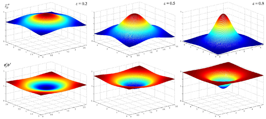
Figure 1: We plot $F^{0}_{12}$ and $\phi^{\dagger}_{f}\phi^{f}$ for different Areas. When $A=A_{c}$ ($\epsilon=0$) the solutions are trivial. When $A\to\infty$ ($\epsilon\to 1$) non-Abelian vortices on the plane are recovered. We plot solutions for different values of $\epsilon$. The area is written in units of $\frac{2}{e^{2}\xi}$.

In the left panel of Figure 2 we show the magnetic field for the $\epsilon\to 1$ case, which corresponds to an elementary ($(1,0)$) non-Abelian vortex on the plane. The ansatz and the numerical method work as well for the study of multi vortex configurations, even when the vortices are not superimposed. We show in the right panel of Figure 2 a $(2,0)$-vortex configuration in the limit $\epsilon\to 1$.

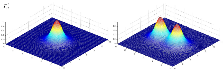
Figure 2: We plot elementary and non-elementary 2-vortex configurations in the large area limit ($A\gg A_{c}$). The model has gauge group $U(1)\times SU(2)$.

6 $U(1)\times SU(N)$ strings

In this section we extend the analysis to the $N>2$ case, with $N_{f}=N$. We start from the Bogomolnyi equations (31)-(32) and consider a non-elementary $(n,0,\dots,0)$ vortex

$$F_{ij}^{0} = -\left(\phi^{\dagger}_{f}\phi^{f}-N\right)\epsilon_{ij}$$

$$F^{m}_{ij} = i\sqrt{2N}\kappa^{2}\phi^{\dagger}_{f}t^{m}\phi^{f}\epsilon_{ij}\ ,$$ (74)

where again $\kappa$ is the ratio of the coupling constants, $\kappa=g/e$. Other elementary vortices like $(0,n,\dots,0)$, etc. can be analogously treated.

We write the $N_{f}=N$ flavor multiplets $\phi^{f}_{i}$ in the form

$$\phi^{1}_{1} = {\cal N}_{1}\exp\left(-\frac{1}{\sqrt{2N}}\left(\eta^{0}-\sqrt{N-1}\eta^{1}\right)\right)\chi_{11}$$

$$\phi^{2}_{2}=\dots=\phi^{N}_{N} = {\cal N}_{2}\exp\left(-\frac{1}{\sqrt{2N}}\left(\eta^{0}+\frac{1}{\sqrt{N-1}}\ \eta^{1}\right)\right)\ ,$$ (75)

where $\chi_{11}$ is defined in (23), and $\eta^{0}$ and $\eta^{1}$ (all other $\eta$’s are taken to be zero) are defined in (37). With this ansatz, and defining

$$h^{+}=\frac{1}{N}\left(\eta^{0}+\frac{1}{\kappa^{2}\sqrt{N-1}}\ \eta^{1}\right)\ ,\ \ \ \ \ \ \ h^{-}=\frac{1}{N}\left(\eta^{0}-\frac{\sqrt{N-1}}{\kappa^{2}}\eta^{1}\right)$$ (76)

we are able to rewrite equations (74) as

$$\nabla^{2}h^{+} = \left(1-\frac{\gamma^{0}(1-\kappa^{2})}{\kappa^{2}L_{1}L_{2}N}\right)-{\cal N}_{2}^{2}\exp\left(-\sqrt{\frac{2}{N}}\left((N-(1-\kappa^{2}))h^{+}+(1-\kappa^{2})h^{-}\right)\right)$$ (77)

$$\nabla^{2}h^{-} = \left(1+\frac{\gamma^{0}}{L_{1}L_{2}N}+\frac{(N-1)\gamma^{0}}{\kappa^{2}L_{1}L_{2}N}\right)$$ (78)

$$- {\cal N}_{1}^{2}|\chi_{11}|^{2}\exp\left(-\sqrt{\frac{2}{N}}\left((N-1)(1-\kappa^{2})h^{+}+(1+\kappa^{2}(N-1))h^{-}\right)\right)\ ,$$

where $\gamma^{0}$ is defined in (15).

As in the $N=2$ case, we notice in equation (78), that since

$$\int_{{\cal T}^{2}}d{\cal T}\nabla^{2}h^{-}=0\ ,$$ (79)

integrating equation (78) on the torus gives

$$\left(1+\frac{\gamma^{0}}{L_{1}L_{2}N}+\frac{(N-1)\gamma^{0}}{\kappa^{2}L_{1}L_{2}N}\right)\int_{{\cal T}^{2}}d{\cal T}\geq 0\ ,$$ (80)

and this again implies the existence of a critical area $A_{c}$ such that

$$A\geq A_{c}\equiv\frac{2\pi n}{N}\sqrt{\frac{2}{N}}\left(1+\frac{N-1}{\kappa^{2}}\right)\ .$$ (81)

We again consider the parameter $\epsilon=1-{A_{c}}/{A}$ in terms of which equations (77)-(78) read

$$\nabla^{2}h^{+} = \left(1+\frac{(1-\epsilon)(1-\kappa^{2})}{N-(1-\kappa^{2})}\right)-{\cal N}_{2}^{2}\exp\left(-\sqrt{2/N}\left((N-(1-\kappa^{2}))h^{+}+(1-\kappa^{2})h^{-}\right)\right)$$ (82)

$$\nabla^{2}h^{-} = \epsilon-{\cal N}_{1}^{2}|\chi_{11}|^{2}\exp\left(-\sqrt{2/N}\left((N-1)(1-\kappa^{2})h^{+}+(1+\kappa^{2}(N-1))h^{-}\right)\right)\ .$$ (83)

For $\epsilon=0$ one has the simple solutions

$${\cal N}_{1}^{2}=0\ ,\ \ \ \ {\cal N}_{2}^{2}=\frac{N}{N-(1-\kappa^{2})}\\$$ (84)

$$h^{+}=h^{-}=0\ .$$ (85)

Non-trivial solutions when $\varepsilon\neq 0$ can be obtained as before, Fourier expanding fields, and further expanding fields in powers of $\varepsilon$. Order to order in $\epsilon$, one is left with recursive relations for the coefficients. These relations can be handled numerically as in the $N=2$ case.

7 Summary and discussion

The main goal of this work was the study of field configurations corresponding to a periodic array of non-Abelian vortices. We have considered a Yang-Mills theory coupled to fundamental scalar matter, a model which can be seen as the truncated bosonic sector of a ${\cal N}=2$ supersymmetric QCD. We have studied these configurations by solving the Bogomolnyi-Prasad-Sommerfeld equations of the theory. By analyzing the (twisted) non-trivial boundary conditions that the fields must satisfy on the two-torus, we were able to propose an ansatz that reduces the BPS equations to a a simpler set of ordinary non linear equations that can be solved numerically. These equations are solved perturbatively in powers of a parameter measuring the departure of the area of the torus from a critical minimal value.

We have presented explicit solutions for the simplest gauge group $U(2)$ which are the natural generalization of the ones studied by Gonzalez Arroyo and Ramos [6] to a non-Abelian Gauge theory. On the other hand, for large areas, our solutions converge to those studied in [11]-[14], for SUSY QCD.

Our work could be extended in several directions. We have analyzed the case in which $N_{f}=N$. A natural extension would be to consider the case in which $N_{f}>N$ to study non-Abelian semi-local strings [23] and this could be of interest in connection with low-energy effective actions for string theories. It is also natural to expect that the same ansatz presented here would work practically in the same way for Chern-Simons-Matter theories [24]-[25], giving in this case origin to configurations of periodic, electrically charged non-Abelian vortices. Also, a similar analysis as the one presented here should be of use to study non-Abelian periodic vortex array configurations presenting BPS equations in the a non-Abelian model with adjoint matter [26], [28] or in the Standard Model [27]. The case considered here corresponds to the particular set of parameters dictated by supersymmetry and BPS equations. It is related, in the Abelian Higgs model, to the limit between Type I and Type II superconductivity, where vortices are non-interacting. Away from this point, the full second order Euler Lagrange equations should be solved. This case, that would correspond to interacting vortices, is technically more involved to study. We expect that there exists a region in parameter space where the vortex-vortex interaction is repulsive giving rise to a lattice of vortices with a definite geometry. We hope to deal with some of this issues in the future.

Acknowledgements: This work was partially supported by ANPCYT (PICT 20204), CICBA, CONICET (PIP 6160), UBA and UNLP (X310).

Appendix

To solve equation (69)

$$\nabla^{2}h^{-}=\epsilon-{\cal N}_{1}^{2}|\chi_{11}|^{2}e^{-2h^{-}}\ ,$$ (86)

we first define

$$H(x_{1},x_{2})=e^{2h^{-}(x_{1},x_{2})}\ ,$$ (87)

and rewrite (86) in complex coordinates $z=x_{1}+ix_{2}$

$$\partial_{z}\left(H^{-1}\partial_{\bar{z}}H\right)=\frac{1}{2}\left(\epsilon-{\cal N}_{1}^{2}|\chi_{11}|^{2}H^{-1}\right)\ .$$ (88)

Since for $\varepsilon=0$ there is a trivial solution

$$H=Constant,\,\,\,\,\,{\cal N}_{1}=0\ ,$$ (89)

and considering that $0\leq\epsilon\leq 1$, we can use $\varepsilon$ as a perturbative parameter and expand $H$ and the normalization constant ${\cal N}_{1}$ in powers of $\varepsilon$

$$H=\sum_{k=0}^{\infty}H_{k}\varepsilon^{k},\ \ \ \ H^{-1}=\sum_{k=0}^{\infty}\bar{H}_{k}\varepsilon^{k},\ \ \ \ {\cal N}_{1}^{2}=\sum_{k=0}^{\infty}N_{k}\varepsilon^{k}\ .$$ (90)

The coefficients $H_{k}$ and $\bar{H}_{k}$ are periodic functions and can then be Fourier expanded

$$H_{k}=\ \sum_{n_{1}n_{2}}h_{n_{1}n_{2}}^{(k)}e^{2\pi i(n_{1}x_{1}/L_{1}+n_{2}x_{2}/L_{2})},\,\,\,\,\,\bar{H}_{k}=\ \sum_{n_{1}n_{2}}\bar{h}_{n_{1}n_{2}}^{(k)}e^{2\pi i(n_{1}x_{1}/L_{1}+n_{2}x_{2}/L_{2})}\ ,$$ (91)

and the same can be done for $|\chi_{11}|^{2}$

$$|\chi_{11}|^{2}=\ \sum_{n_{1}n_{2}}\eta_{n_{1}n_{2}}e^{2\pi i(n_{1}x_{1}/L_{1}+n_{2}x_{2}/L_{2})}\ ,$$ (92)

with normalized coefficients such that $\eta_{00}=1$.

Inserting these expansions in eq.(86) one can determine order by order the coefficients,

$$h_{n_{1}n_{2}}^{(0)} = \bar{h}_{n_{1}n_{2}}^{(0)}=\left\{\begin{array}[]{cc}1&n_{1}=\ n_{2}=0\\ 0&n_{1}\neq 0,n_{2}\neq 0\end{array}\right.$$ (95)

$$h_{n_{1}n_{2}}^{(1)} = \left\{\begin{array}[]{cc}0&n_{1}=\ n_{2}=0\\ \frac{2\pi\eta_{n_{1}n_{2}}}{|\xi_{n_{1}n_{2}}|^{2}}&n_{1}\neq 0,n_{2}\neq 0\end{array}\right.$$ (98)

$$\bar{h}_{n_{1}n_{2}}^{(1)} = -h_{n_{1}n_{2}}^{(1)}\ \ \ \ \ \ \ \ \ \ \ \ \ \ \ \ \ \ \ \ \ \ \ \ \ \ \ \ \ \ \ \ \ \ \ \ \ \ \ ,$$ (99)

where

$$\xi_{n_{1}n_{2}}\equiv\pi\sqrt{T}\left(in_{1}+\frac{n_{2}}{\sqrt{T}}\right)\ ,$$ (100)

with ${T}=L_{2}/L_{1}$ the aspect ratio of the torus. In the same way one can calculate coefficients to any order $Q$ in $\varepsilon$

$$h_{n_{1}n_{2}}^{(Q)}=\left\{\begin{array}[]{cc}0&n_{1}=\ n_{2}=0\\ \frac{C_{n_{1}n_{2}}^{(A)}-C_{n_{1}n_{2}}^{(B)}-C_{n_{1}n_{2}}^{(C)}}{|\xi_{n_{1}n_{2}}|^{2}}&n_{1}\neq 0,n_{2}\neq 0\end{array}\right.\ ,$$ (101)

with

$$C_{q_{1}q_{2}}^{(A)}\!\!\! = \!\!\!\sum_{n_{1}n_{2}}\sum_{k=1}^{Q-1}\ \bar{h}_{n_{1}n_{2}}^{(k)}\ h_{q_{1}-n_{1},q_{2}-n_{2}}^{(Q-k)}\ \xi_{q_{1}q_{2}}\ \bar{\xi}_{q_{1}-n_{1},q_{2}-n_{2}}$$

$$C_{q_{1}q_{2}}^{(B)}\!\!\! = \!\!\!2\pi\sum_{n_{1}n_{2}}\sum_{k=0}^{Q-1}\ \bar{h}_{n_{1}n_{2}}^{(k)}\ N_{Q-k}\ \eta_{q_{1}-n_{1},q_{2}-n_{2}}$$

$$C_{q_{1}q_{2}}^{(C)}\!\!\! = \!\!\!\sum_{n_{1}n_{2}}\sum_{k=0}^{Q-2}\ \bar{h}_{n_{1}n_{2}}^{(k)}\ h_{q_{1}-n_{1},q_{2}-n_{2}}^{(Q-k-1)}\ \xi_{q_{1}q_{2}}\ \bar{\xi}_{q_{1}-n_{1},q_{2}-n_{2}}\ .$$

Coefficients ${\bar{h}}_{n_{1}n_{2}}$, appearing in the expansion of $H^{-1}$, are obtained from the condition $HH^{-1}=1$

$$\bar{h}^{(Q)}_{q_{1}q_{2}}=-\sum_{n_{1}n_{2}}\sum_{k=1}^{Q}\ h^{(k)}_{n_{1}n_{2}}\ \bar{h}^{(Q-k)}_{q_{1}-n_{1},q_{2}-n_{2}}\ .$$ (102)

One also has to find a recurrence relation for the coefficients $N_{k}$. For this, the condition $\int_{{\cal T}^{2}}d{\cal T}\tilde{F}_{12}=0$ implies

$$N_{0} = 0\ ,\ \ \ \ \ \ \ N_{1}=1$$

$$N_{Q} = -\sum_{n_{1}n_{2}}\sum_{k=1}^{Q-1}\ \eta_{-n_{1},-n_{2}}\ \bar{h}_{n1n2}^{(k)}\ N_{Q-k}\ ,\;\;\;Q>1\ .$$

Computing these recursive relations we can obtain $h^{-}$ and ${\cal N}_{1}$, and with this compute the magnetic and Higgs field from eqs.(72)-(73).

References

[1]
H. B. Nielsen and P. Olesen,
Nucl. Phys. B 61, 45 (1973).
[2]
E. B. Bogomolnyi,
Sov. J. Nucl. Phys. 24 (1976) 449
[Yad. Fiz. 24 (1976) 861].
[3]
H. J. de Vega and F. A. Schaposnik,
Phys. Rev. D 14 (1976) 1100.
[4] C. H. Taubes, Comm. Math. Phys. 72
(1980) 277.
[5] S. B. Bradlow,
Commun. Math. Phys. 135 (1990) 1 17.
[6]
A. Gonzalez-Arroyo and A. Ramos,
JHEP 0407 (2004) 008
[7]
D. Tong,
Lectures at TASI 2005,
arXiv:hep-th/0509216.
[8] F.A. Schaposnik,
Lectures at 4th Advanced Chilean School of Astrophysics, Cosmology and
Gravitation, Valparaiso, Dec 2006.
arXiv:hep-th/0611028.
[9]H. J. de Vega and F. A. Schaposnik,
Phys. Rev. Lett. 56 (1986) 2564;
Phys. Rev. D 34 (1986) 3206.
[10]
A. Hanany and D. Tong,
JHEP 0307, 037 (2003)
[arXiv:hep-th/0306150].
[11]
R. Auzzi, S. Bolognesi, J. Evslin, K. Konishi and A. Yung,
Nucl. Phys. B 673 (2003) 187
[12]
A. Hanany and D. Tong,
JHEP 0404, 066 (2004)
[13] M. Shifman and A. Yung,
Phys. Rev. D 70 (2004) 045004
[14]
A. Gorsky, M. Shifman and A. Yung,
Phys. Rev. D 71 (2005) 045010
[15]
M. Eto, Y. Isozumi, M. Nitta, K. Ohashi and N. Sakai,
Phys. Rev. Lett. 96 (2006) 161601
[16]
M. Eto, Y. Isozumi, M. Nitta, K. Ohashi and N. Sakai,
J. Phys. A 39 (2006) R315
[17] M. Shifman and A. Yung,
arXiv:hep-th/0703267.
[18]
A. Gonzalez-Arroyo, Talk at the Summer School on Nonperturbative Quantum Field Physics,
Peniscola, Spain,
arXiv:hep-th/9807108.
[19]
G. ’t Hooft,
Nucl. Phys. B 153 (1979) 141.
[20]
J. D. Edelstein, C. Nunez and F. Schaposnik,
Phys. Lett. B 329 (1994) 39
[21] A. Gonzalez-Arroyo and A. Ramos,
JHEP 0701 (2007) 054
[22]P. Forgacs, G.S. Lozano, E.F. Moreno, F.A. Schaposnik,
JHEP 0507 (2005) 074;
G. S. Lozano, D. Marques and F. A. Schaposnik,
JHEP 0609, 044 (2006)
[23]
M. Shifman and A. Yung,
Phys. Rev. D 73 (2006) 125012
[24]
L. G. Aldrovandi and F. A. Schaposnik,
arXiv:hep-th/0702209.
[25]
G. S. Lozano, D. Marques, E. F. Moreno and F. A. Schaposnik,
arXiv:0704.2224 [hep-th].
[26]
H. J. de Vega and F. A. Schaposnik,
Phys. Rev. Lett. 56 (1986) 2564.
[27]J. Ambjorn and P. Olesen, Int. J. Mod. Phys. A5 (1990) 4525; Nucl. Phys. B330, (1990) 193;
G. Bimonte and G. Lozano,
Phys. Rev. D 50 (1994) 6046; Y. Yang,
Physica D101 (1997) 57.