Embedding Spacetime via a Geodesically Equivalent Metric of Euclidean Signature
Rickard Jonsson

Submitted: 2000-11-06, Published: July 2001
Journal Reference: Gen. Rel. Grav. 33 1207
Abstract. Starting from the equations of motion in a 1 + 1 static, diagonal, Lorentzian spacetime, such as the Schwarzschild radial line element, I find another metric, but with Euclidean signature, which produces the same geodesics $x(t)$. This geodesically equivalent, or dual, metric can be embedded in ordinary Euclidean space. On the embedded surface freely falling particles move on the shortest path. Thus one can visualize how acceleration in a gravitational field is explained by particles moving freely in a curved spacetime. Freedom in the dual metric allows us to display, with substantial curvature, even the weak gravity of our Earth. This may provide a nice pedagogical tool for elementary lectures on general relativity. I also study extensions of the dual metric scheme to higher dimensions.
KEY WORDS: Embedding spacetime, dual metric, geodesics, signature change

1 Introduction

It is easy to display the meaning of curved space. For instance we may display the spatial curvature created by a star using an embedding diagram. Figs. 1 & 2.

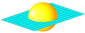
Figure 1: A symmetry plane through a star.

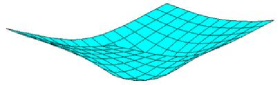
Figure 2: The embedding diagram.

When it comes to displaying curved spacetime things become more difficult. The acceleration of a free test particle is due to a curvature of spacetime. What does it mean to have curved time, and can we display it somehow?

When we create the embedding diagram for the space of a symmetry plane through a star, we make a mapping from our spatial plane onto a curved surface embedded in Euclidean space. This is done so that distances as measured by rulers are the same on the symmetry plane as on the embedding diagram. The difference is that on the symmetry plane there is a metric function giving the true distance between points whereas in the embedding diagram it is the shape of the surface that gives us the distances.

If we want to do the same thing for a 1+1 spacetime we immediately run into trouble. We have null distances between points and even negative squared distances. In the Euclidean space, that we are used to embed in, we can never have negative distances.

Instead of distances, maybe we should study motion. For geodesic lines of freefallers in the ordinary spacetime picture of a Schwarzschild black hole there is nothing special, or singular, with null geodesics for instance. Would it be possible to find a mapping from our coordinate plane to a curved surface such that all the worldlines corresponding to test particles in free fall, are geodesics (moving on the shortest distance) on the curved surface? See Fig. 3.

Figure 3: A mapping to a surface where all freefallers take the shortest path.

Alternatively, if we can not do it for all particles, can we do it for some set of geodesics, like photon-geodesics?

Suppose that we have found a mapping onto a curved surface such that all freefallers move between fixed points like a tightened thread, i.e. on the shortest path. Between nearby points on this surface there is then a Euclidean distance as measured with a ruler. This means that we can assign a Euclidean distance for small displacements in our coordinates. Thus, on our original coordinate plane we imagine there to live, not only a Lorentzian metric, but also a Riemannian metric, that both produce the same geodesics.

With this understanding, the problem of finding a surface with the right curvature is reduced to finding a Riemannian metric that produces the right set of geodesics $x(t)$. Once we have found such a geodesically dual metric, if it exists, we can hopefully embed and visualize, a curved spacetime.

For some special geometries we know that the dual metric exists. In particular, starting from a flat Minkowski spacetime and using standard coordinates, the geodesic lines on the coordinate plane are just straight lines. This is also the case if we have an ordinary Euclidean metric. In this case we can thus just flip the sign of the spatial part of the Minkowski metric to find a dual metric. The embedding of a two-dimensional Minkowski spacetime will thus simply be a plane.

Also, in a general Lorentzian spacetime, we can at every point choose coordinates so that the metric reduces to Minkowski, with vanishing derivatives. In this local, freely falling, coordinate system particles move on straight lines. This means that they move on the longest path in the local Lorentzian spacetime. However they also move on the shortest path in the corresponding local Euclidean spacetime. Then we know that there exists a dual metric that produces the right equations of motion at least in every single point. The question is whether we can connect all these single point metrics in a smooth way.

Notice that constant time lines for inertial observers in Minkowski, are straight lines. They are also geodesics, moving the longest path, if we change the sign of the whole metric so that spacelike distances becomes positive. This means that if we find a dual metric, there will be geodesics that correspond to local time lines of freefallers. We may also consider these lines to be particles moving faster than light, so called tachyons.

On the curved surface there is in principle no way to distinguish between timelike and spacelike displacements from the shape of the surface. However, on the surface lives the original Lorentzian metric that tells us the true distances between nearby points. In other words there are small Minkowski systems living on the surface, telling us the proper distance between points.

In a sense all we are doing is shaping the manifold. We still need the ordinary metric to get distances right. The difference is that we do not need this function to get the geodesics right. This follows from the shape of the surface.

2 The dual metric in $1+1$ dimensions

Let us for simplicity, start the analysis with a 1+1 time independent diagonal metric, with Lorentzian signature, and see if we can find a time independent and diagonal dual metric with Euclidean signature.

2.1 Equations of motion

Assume that we have a line element:

$$d\tau^{2}=a(x)\cdot dt^{2}+c(x)\cdot dx^{2}$$ (1)

Using the squared Lagrangian formalism (see e.g. [5]), we immediately get the integrated equations of motion:

$$a\left(\frac{dt}{d\tau}\right)^{2}+c\left(\frac{dx}{d\tau}\right)^{2} = 1$$ (2)

$$a\frac{dt}{d\tau} = K$$ (3)

Here $K$ is a constant for every geodesic. Now we want to find an equation for $x(t)$. Introducing $\sigma=1/K^{2}$ for compactness, the result is:

$$\left(\frac{dx}{dt}\right)^{2}=\frac{a}{c}\left(\sigma\ a-1\right)$$ (4)

Notice that this equation applies to both $(+,-)$ and $(+,+)$ metrics.

2.2 The dual metric equations

The question is now: What other metrics, if any, can produce the same set of geodesics $x(t)$? Denoting the original metrical components by $a_{0}$ and $c_{0}$ and the original constant of the motion for a certain geodesic by $\sigma_{0}$ we must have:

$$\frac{a}{c}(\sigma a-1)=\frac{a_{0}}{c_{0}}(\sigma_{0}a_{0}-1)$$ (5)

This relation must be fulfilled for every $x$ and every geodesic. Notice that $\sigma$ may depend on $\sigma_{0}$ only.

We see immediately that we can regain the old metric simply by setting $a=a_{0}$, $c=c_{0}$ and $\sigma(\sigma_{0})=\sigma_{0}$. As for other solutions they may appear hard to find at first. We know however that starting from e.g. Minkowski, we must be able to flip the sign on the spatial part of the metric, without affecting the geodesic lines. Let us however rewrite Eq. (5) a bit:

$$\sigma=\left(\frac{c}{c_{0}}\frac{a_{0}^{2}}{a^{2}}\right)\cdot\sigma_{0}+\left(\frac{1}{a}-\frac{c}{c_{0}}\frac{a_{0}}{a^{2}}\right)$$ (6)

Now we see more clearly that if this relation is to hold for all $x$ and all $\sigma_{0}$ we must have:

$$k_{1}=\frac{c}{c_{0}}\frac{a_{0}^{2}}{a^{2}}\qquad\qquad k_{2}=\frac{1}{a}-\frac{c}{c_{0}}\frac{a_{0}}{a^{2}}$$ (7)

We have thus a linear relation between the constants of the motion:

$$\sigma=k_{1}\cdot\sigma_{0}+k_{2}$$ (8)

Here $k_{1}$ and $k_{2}$ are constants that depend on neither $x$ nor $\sigma_{0}$. From Eq. (7) we may solve for $a$ and $c$ in terms of $k_{1}$ and $k_{2}$:

$$a=\frac{a_{0}}{a_{0}k_{2}+k_{1}}\qquad\qquad c=\frac{c_{0}k_{1}}{\left(a_{0}k_{2}+k_{1}\right)^{2}}$$ (9)

Defining $\alpha=1/k_{2}$ and $\beta=-k_{1}/k_{2}$ this may be rewritten as:

$$a = \alpha\frac{a_{0}}{a_{0}-\beta}$$ (10)

$$c = \alpha\frac{-c_{0}\beta}{\left(a_{0}-\beta\right)^{2}}$$ (11)

We see that $\alpha$ is a pure scaling constant whereas $\beta$ is connected to compression along the $x$-axis as will be discussed later.

Now the question is: can we choose $\alpha$ and $\beta$ so that, assuming a Lorentzian original metric (positive $a_{0}$ and negative $c_{0}$) we get a Riemannian dual metric? Indeed necessary and sufficient conditions for the dual metric to be positive definite is:

$$0<\alpha$$ (12)

$$0<\beta<a_{0}$$ (13)

2.3 The Schwarzschild exterior metric

Introducing dimensionless and rescaled coordinates $x=\frac{r}{2MG}$ and correspondingly rescaling Schwarzschild and proper time, the ordinary Schwarzschild metric is given by:

$$a_{0}=\left(1-\frac{1}{x}\right)\qquad\qquad c_{0}=-\left(1-\frac{1}{x}\right)^{-1}$$ (14)

At spatial infinity this reduces to $a_{0}=1$ and $c_{0}=-1$. At infinity our new metric is thus reduced to:

$$a_{\infty}=\alpha\frac{1}{1-\beta}\qquad\qquad c_{\infty}=\alpha\frac{\beta}{\left(1-\beta\right)^{2}}$$ (15)

Let us study the quotient of $a_{\infty}$ and $c_{\infty}$:

$$\frac{a_{\infty}}{c_{\infty}}=\frac{1}{\beta}-1$$ (16)

We see that for $\beta>1/2$ the quotient is smaller than 1. This implies a stretching in $x$. When we embed our new metric this will correspond to opening up the photon lines so they become more parallel to the constant time line.

In particular, demanding that $a_{\infty}=1$ and $c_{\infty}=1$ yields $\alpha=1/2$ and $\beta=1/2$. Using this particular gauge, from now on denoted the standard gauge, we get from Eq. (10) and Eq. (11) the dual line element:

$$ds^{2}=\frac{x-1}{x-2}\cdot dt^{2}+\frac{x^{3}}{(x-1)(x-2)^{2}}\cdot dx^{2}$$ (17)

This metric has positive metrical components from infinity and in to $x=2$. We have thus succeeded, and found a Riemannian dual metric, at least on a large section of the spacetime.

2.4 On the interpretation of $\alpha$ and $\beta$

We may rewrite Eq. (10) and Eq. (11) as:

$$\frac{a}{\alpha}=\frac{a_{0}/\beta}{a_{0}/\beta-1}\qquad\qquad\frac{c}{\alpha}=\frac{-c_{0}/\beta}{\left(a_{0}/\beta-1\right)^{2}}$$ (18)

Then we see that just as $\alpha$ is a rescaling of the new metric – so is $\beta$ a rescaling of the original metric. We can easily work out the inverse of the relations above to find:

$$\frac{a_{0}}{\beta}=\frac{a/\alpha}{a/\alpha-1}\qquad\qquad\frac{c_{0}}{\beta}=\frac{-c/\alpha}{\left(a/\alpha-1\right)^{2}}$$ (19)

We see that we have a perfect symmetry in going from the original metric to the dual and vice versa, justifying the duality notion. This symmetry would be even more obvious if we would denote $\beta$ by $\alpha_{0}$ instead.

With hindsight we realize that we must have two rescaling freedoms just like that. A metric that is dual to some original metric must also be dual to a twice as big original metric and vice versa. Notice however that if we make the original space twice as big, then the dual space does not automatically become twice as big. It does however if we double both $\alpha$ and $\beta$!

3 The embedding equations

In general if we have a metric with a symmetry, we can embed it as a rotational surface if we can embed it at all. Our task is then to find a radius $r(x)$ and a height $z(x)$ for the embedding of the dual metric. See Fig. 4.

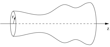
Figure 4: A rotational surface.

3.1 Finding $r(x)$

For pure $t$-displacements the dual distance traveled is $ds=\sqrt{a}\cdot dt$. We realize that we must have:

$$r=k\sqrt{a}$$ (20)

Here $k$ is a constant of the embedding only, it does not affect the way we measure distances on the surface – only its shape. See Section 3.4. In terms of the original metric:

$$r=k\cdot\sqrt{\alpha\frac{a_{0}}{a_{0}-\beta}}$$ (21)

In particular for the Schwarzschild case using the standard gauge ($\alpha=1/2$, $\beta=1/2$), and $k=1$:

$$r(x)=\sqrt{\frac{x-1}{x-2}}$$ (22)

We see that as $x$ tends to infinity we have a unit radius, whereas approaching $x=2$ from infinity the radius blows up. Already now we may understand the qualitative behavior of the embedding diagram. The curious reader may jump immediately to Section 4.

3.2 Finding $z(x)$

From Fig. 5 using the Pythagorean theorem we find:

Figure 5: The relation between $dz$, $dr$ and $dl$.

$$dz=dx\cdot\sqrt{c(x)-\left(\frac{dr(x)}{dx}\right)^{2}}$$ (23)

Using Eq. (11) and Eq. (21) and defining ${a^{\prime}_{0}}=da_{0}/dx$ we readily get:

$$dz=dx\cdot\sqrt{\alpha\frac{-c_{0}\beta}{(a_{0}-\beta)^{2}}-\frac{k^{2}\alpha\beta^{2}}{4}\cdot\frac{{a^{\prime}_{0}}^{2}}{a_{0}(a_{0}-\beta)^{3}}}$$ (24)

So:

$$\Delta z=\sqrt{\alpha}\sqrt{\beta}\int dx\sqrt{\frac{-c_{0}}{(a_{0}-\beta)^{2}}-\frac{k^{2}\beta}{4}\cdot\frac{{a^{\prime}}_{0}^{2}}{a_{0}(a_{0}-\beta)^{3}}}$$ (25)

3.3 Embedding criterions

We see from Eq. (25) that there is a limit as to how big the embedding constant $k$ can be lest we get something negative within the root:

$$k^{2}<\textrm{min}\left\{-c_{0}\frac{4}{\beta}\frac{a_{0}(a_{0}-\beta)}{(a^{\prime}_{0})^{2}}\right\}$$ (26)

Let us investigate what this restriction amounts to for the specific cases of the Schwarzschild exterior and interior metric.

3.3.1 The exterior metric

For the exterior Schwarzschild metric, the expression within the brackets of Eq. (26) is smaller the closer to the gravitational source that we are, approaching 0 before we reach the horizon. On the other hand it goes to infinity as $x$ goes to infinity, since $a^{\prime}_{0}$ goes to zero here. This means that, for any given $k$, the embedding works, as we approach infinity. It however only works from a certain point in $x$ and onwards.

For the exterior Schwarzschild we have:

$$a_{0}=1-\frac{1}{x}\qquad\qquad a^{\prime}_{0}=\frac{1}{x^{2}}\qquad\qquad-c_{0}=\left(1-\frac{1}{x}\right)^{-1}$$ (27)

After some minor juggling we then find:

$$k<\frac{2x^{2}}{\sqrt{\beta}}\sqrt{1-\beta-\frac{1}{x}}$$ (28)

Assuming that we are using the standard gauge, $\beta=1/2$, and $k=1$ this reduces to a restriction in $x$:

$$x^{3}(x-2)>\frac{1}{4}\qquad\Rightarrow\qquad x>2,02988...$$ (29)

So, using the standard gauge, the dual embedding only exists from roughly two Schwarzschild radii and on towards infinity. Incidentally may insert this innermost $x$ into Eq. (22) and find $r\sim 5.87$.

Notice that these numbers only apply to the particular boundary condition where we have Pythagoras and unit embedding radius at infinity. By choosing other gauge constants and embedding constants we can embed the spacetime as close to the horizon as we want. Notice that there is nothing physical with the limits of the dual metric and the embedding limit. They are merely unfortunate artifacts of the theory.

3.3.2 The interior metric of a star

Assuming a static, spherically symmetric star consisting of a perfect fluid of constant proper density, we have the standard Schwarzschild interior metric:

$$a_{0} = \frac{1}{4}\left(3\sqrt{1-\frac{1}{x_{0}}}-\sqrt{1-\frac{x^{2}}{x_{0}^{3}}}\right)^{2}$$ (30)

$$c_{0} = -\left(1-\frac{x^{2}}{x_{0}^{3}}\right)^{-1}$$ (31)

Here $x_{0}$ is the $x$-value at the surface of the star. For the interior star the embedding criterion, Eq. (26), becomes:

$$k^{2}<\frac{4x_{0}^{6}}{\beta}\textrm{min}\left\{\frac{1}{x^{2}}\cdot\left(a_{0}-\beta\right)\right\}$$ (32)

The bracketed function can be either monotonically decreasing, have a local minima within the star or even be monotonically increasing depending on $x_{0}$ and $\beta$.

Apart from the embedding restriction we have of course the restriction on the metric itself. Since $a_{0}$ is monotonically increasing, for interior plus exterior metric, the metrical restriction for the entire star becomes:

$$\beta<a_{0}(0)$$ (33)

Using $\beta=1/2$ and the interior $a_{0}$ in the center of the star this restriction becomes a restriction in $x_{0}$:

$$x_{0}>\frac{9}{9-(\sqrt{2}+1)^{2}}\simeq 2,838$$ (34)

For any $x_{0}>2,837$ and $\beta=1/2$ the right hand side of Eq. (32) is always considerably larger than $1$ and thus the embedding imposes no extra constraints on $x_{0}$ in the gauge in question, assuming $k=1$. Incidentally we see from Eq. (21) that the radius of the central bulge goes to infinity as $x_{0}$ approaches its minimal value.

3.4 On the interpretation of the embedding constant $k$

Recall Eq. (20):

$$r(x)=k\sqrt{a(x)}$$ (35)

We see that $k$ determines the scale for the embedding radii. Notice however that the distance to walk between two radial circles, infinitesimally displaced, is determined by $dl=\sqrt{c}dx$. So, when we double $k$ we double the radius of all the circles that make up the rotational body while keeping the distance to walk between the circles unchanged. This means that we increase the slope of the surface everywhere. The more slope the bigger the increase of the slope. If we increase $k$ too much the embedding will fail. An example of how different $k$ affects a certain embedding is given in Fig. 6.

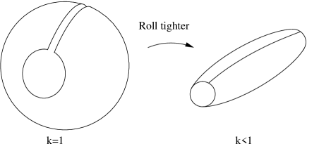
Figure 6: Two isometric embeddings of a sliced-open sphere.

Now consider Eq. (21):

$$r(x)=k\sqrt{\alpha}\sqrt{\frac{a_{0}}{a_{0}-\beta}}$$ (36)

We notice that, while increasing $k$ we can decrease $\alpha$ in such a way that we do not change any $r(x)$.

The net effect on the embedding is then to compress the surface in the $z$-direction, while keeping all radii. This is done in such a way that all distances $(dl)$ on the surface in the $z$-direction is reduced by the same factor everywhere. This means that where the slope is big we compress a lot in the $z$-direction. Also since we are rescaling the dual metric, meter- and second-lines on the surface will move closer. Using this scheme we can produce substantial curvature out of something that was originally almost cylindrical. Also, using our $\beta$-freedom, we can flip down the photon lines towards the time line to better suit what we humans experience. This way we have a chance of displaying, with reasonable distances and curvatures, why things accelerate at the surface of the Earth. See Section 7.

4 The embedding diagram

Already from Eq. (22) we realize quantitatively how the new dual $(+,+)$ spacetime must look like. See Fig. 7. Notice that time is the azimuthal angle and the whole spacetime is layered (infinitely thin), like a toilet roll.

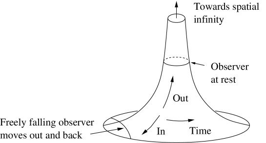
Figure 7: A vision of spacetime.

The geometry will approach a cylinder as we go towards spatial infinity. This is as it should be since we want a flat spacetime where there is no gravity.

Notice that in an ordinary embedding of an equatorial plane of a black hole, the geometry opens up towards infinity and the little hole is at the horizon. Here it opens up towards the horizon and the little hole is towards infinity.

So, we have found a dual $(+,+)$ spacetime of Schwarzschild, that can be embedded, where all particles move on geodesics, i.e. shortest distance. We can thus make a real model, say in polished metal, and then find possible geodesics just by tightening a thin thread between pairs of points on the surface.

Alternative to tightening threads, one could put a little toy car or motorcycle, on the surface. Starting the car at some point, directed solely in the azimuthal direction, and pushing the car straight forward will result in a spiral inwards. Thus we see how moving straight forward can result in acceleration. Also, if we want the car to stay at a fixed $x$ we notice that we must turn the wheel (assuming an advanced toy car), so that the car is constantly turning left (e.g.), i.e. accelerating upwards. This illustrates in an excellent manner how it is possible for us Earthlings to always accelerate upwards without ever going anywhere.

Now that we have understood the name of the game in this embedding scheme we can figure out qualitatively how the embedded spacetime of a line through a star must look like. This is depicted in Fig. 8. For better layout, and also to more naturally connect the embedding diagram to the ordinary Schwarzschild diagram, we have now space in the left-right direction.

Figure 8: The spacetime of a central line through a star.

A particle oscillating around the center of the star is nothing but a thread winding around the central bulge. Notice however that we do not generally expect to have something close to a sphere for the interior embedding. For a non-compact star we would rather expect something close to a cylinder, with a long slightly bulged interior star. Also, if we would have a perfect sphere for the the interior, then oscillations around the center of the star would correspond to great circles. This would mean that the period of revolution, as measured in Schwarzschild time, would be independent of the amplitude of the oscillation. This is actually true, for a constant density star, in Newtonian theory. In the full theory, and for more general density distributions, we will not expect a perfect sphere however. Also, more embeddings than the sphere has the focusing feature that makes the period of revolution independent of the amplitude.

How a certain density can affect the shape of the interior bulge is depicted in Fig. 9.

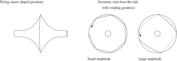
Figure 9: How the shape of the bulge, due to the density distribution, affects the the amplitude dependence of the periods of revolution for freefallers around the center of the star.

In this geometry it is obvious that increasing amplitude means increasing period of revolution. This is exactly what may be expected from Newtonian theory if the density is increasing towards the center. We may also consider the opposite situation with decreasing density in the center of the star. Then the central parts of the embedding will be close to cylindrical, and it is easy to imagine that increasing amplitude means decreasing period of revolution. Notice however that if we want to find the exact dependence of $x(t)$, from the embedding diagram, we need also to know how the $x$’s are distributed on the surface.

It is fascinating that we can visualize how density creates spacetime curvature, which in turn affects the geodesics of particles

4.1 Numerically calculated diagrams

Numerically it is no problem to integrate Eq. (25). For the exterior metric a particular result is depicted in Fig. 10.

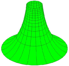
Figure 10: A standard embedding of the exterior spacetime of a star for $2.03<x<3.00$. The spatial lines are equidistant in $x$ with a spacing that is one fourth of the spacing between the time lines (for esthetical reasons).

We may as easily get the embedding for the full star. One result of this, where we have omitted the coordinate lines, is depicted in Fig. 11.

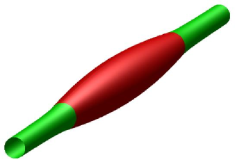
Figure 11: A standard embedding of the spacetime of a star with $x_{0}\sim 3.2$.

One may reflect that the embedding is not as bulgy as expected, and still I have chosen a compactness for which it is about as bulgy as it gets for a standard embedding.

The main reason for the flatness is that as one moves towards the center of the star and the embedding radius is increasing, photon geodesics (and other geodesics) will be tilted further towards the constant time line. This is a direct effect of photons moving the shortest distance on the rotational surface (see Section 6). Also as the radius increases, moving in Schwarzschild time, means moving a longer distance on the surface, remember that the Schwarzschild time is proportional to the azimuthal angle. These two radial effects means that $dz/dt$, for photon geodesics, increases with increasing $r$. We therefore understand that we must stretch the bulge in the $z$-direction to insure that photons do not pass the star too quickly.

If we want a star with more shape we can increase the $k$-value. This increases the tilt of the surface everywhere, making the embedding bulgier while photon lines at infinity remains at $45^{o}$.

5 The weak field limit

The dual metric and the embedding formulae are rather mathematically complicated, especially for the interior star. To gain some intuition it will prove worthwhile to study the weak field limit, where we can Taylor expand our expressions. In this section we will not use rescaled coordinates, $x$, but the ordinary radius, denoted by $\rho$ so as not to confuse it with the embedding radius $r$. Let us use the standard gauge $\alpha=\frac{1}{2}$, $\beta=\frac{1}{2}$ and also $k=1$ for simplicity. We define:

$$a_{0}=1-\varepsilon(\rho)$$ (37)

Assuming $\varepsilon(\rho)$ to be small we may Taylor expand the expression for the embedding radius:

$$r = k\sqrt{\alpha}\sqrt{\frac{a_{0}}{a_{0}-\beta}}\qquad\Rightarrow\qquad r\simeq 1+\frac{\varepsilon}{2}$$ (38)

Introducing $r=1+h$, we have thus to lowest order $h=\varepsilon/2$. One may show [3] that for a stationary, weak field in general we have:

$$a_{0}=(1+2\cdot\phi)$$ (39)

Here $\phi$ is the dimensionless (using $c_{\textrm{\tiny light}}=1$) Newtonian potential per unit mass, e.g. $GM/\rho$ for a point mass. We thus conclude that:

$$h=-\phi$$ (40)

So in first order theory, using the standard gauge and $k=1$, the height of the perturbation equals exactly minus the Newtonian potential. This result is actually not to surprising. See section 6.

Incidentally we may also show that:

$$\begin{array}[]{rclrcl}\begin{array}[]{ll}a_{0}=1-\varepsilon(\rho)\\[-5.69054pt] c_{0}=-(1+\delta(\rho))\end{array}\qquad\Rightarrow\qquad z\simeq\int d\rho\ 1+\displaystyle\frac{\delta(\rho)}{2}+\displaystyle\frac{\varepsilon(\rho)}{2}\end{array}$$ (41)

5.1 Applications

We may use our newly found intuition from Newtonian theory to create a new interesting picture. Suppose that we have a static spherical shell of some mass. Inside the shell we have no forces and thus $\phi$ is constant. According to the derivation above we would then have constant $h$ in the interior of the star. See Fig. 12.

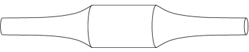
Figure 12: The rolling-pin spacetime of a central line through a Newtonian shell of matter.

We see that inside the shell the geometry is flat, consistent with having no gravitational forces.

I will leave to the reader to figure out what strange spherical mass distribution that could give rise the the embedding diagram depicted in Fig. 13.

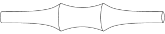
Figure 13: The spacetime of a central line through a certain energy distribution.

6 On geodesics on rotational surfaces

Since this paper utilizes geodesics on rotational surfaces – maybe a general note on the subject is in order. Parameterizing any rotational surface with $r$ and $\varphi$, the metric can be written (in every region of monotonically increasing or decreasing $r$):

$$ds^{2}=r^{2}\cdot d\varphi^{2}+f(r)\cdot dr^{2}$$ (42)

Using the squared Lagrangian formalism we immediately get the integrated equation of motion:

$$r^{2}\frac{d\varphi}{ds}=\textrm{const}$$ (43)

Letting $\theta$ denote the angle between the geodesic in question and a purely azimuthally directed line we may rewrite Eq. (43) into:

$$r\cdot\cos(\theta)=\textrm{const}$$ (44)

In particular we see that the tilt of a certain geodesic is completely determined by the radius, and that the tilt of the geodesic line increases with increasing radius. By considering a thread tightened on the surface we understand that this is very reasonable.

Assuming the rotational surface to be a small perturbation of a cylinder of unit radius $r=1+h$, and assuming the tilt ($\theta$) to be small, we may easily prove from Eq. (44) that to lowest order we have:

$$\frac{d^{2}z}{d\varphi^{2}}=\frac{dh}{dz}$$ (45)

Thus one may verify that, at least for small velocities and gravitational fields, one can explain gravitational attraction by motion on a rotational surface.

7 Displaying the Earth gravity

We would like to display why things accelerate at the surface of the Earth. We want a clearly curved surface where meters and seconds correspond to roughly the same distances as the radius of the cone. We have three parameters that determine the shape and size of the embedded surface. Let us therefore make three demands, exactly at the surface of the Earth:

$$\begin{array}[]{rclrclrclrclrclrcl}\sin\Theta_{0}&=&0.8&&&\textrm{The angle of slope for the surface}\\[-2.84526pt] r_{0}&=&1&&&\textrm{The embedding radius}\\[-2.84526pt] \Delta\tau_{\textrm{\tiny real}}&=&1\textrm{s}&&&\textrm{The proper time per circumference}\end{array}$$ (46)

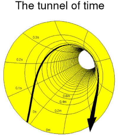
Figure 14: An embedding diagram of the spacetime at the surface of the Earth. We see a freefaller moving up and then down again in perfect agreement with the Newtonian predictions.

From these requirements it is an easy exercise to find the corresponding values of $k$, $\alpha$ and $\beta$. The results are:

$$\begin{array}[]{rclrclrclrclrclrcl}k&=&\displaystyle\frac{\Delta\tau_{\textrm{\tiny real}}c_{\textrm{\tiny l}}}{2\pi\sqrt{a_{\textrm{\tiny e0}}}R_{G}}&&&\sim 5.38\cdot 10^{9}\\ \beta&=&\displaystyle\frac{a_{\textrm{\tiny e0}}}{1+\left(\displaystyle\frac{k}{2\textrm{sin}\Theta_{0}\cdot x_{0}^{2}}\right)^{2}}&&&\sim\displaystyle\frac{a_{\textrm{\tiny e0}}}{1+\underbrace{4.25\cdot 10^{-17}}_{\delta}}\\ \alpha&=&r_{0}^{2}\displaystyle\frac{1}{4x_{0}^{4}\textrm{sin}^{2}\Theta_{0}+k^{2}}&&&\sim 1.47\cdot 10^{-36}\end{array}$$ (47)

Here $a_{e0}=a_{0}(x_{0})$ and $c_{\textrm{\tiny l}}$ is the velocity of light. Since Matlab only operates at 16 decimals, we cannot cope numerically with the expression for $\beta$, Eq. (47). We have to Taylor-expand our expressions for the embedding coordinates $z$ and $r$. Limiting ourselves to the exterior metric, and introducing $\Delta x=x-x_{0}$ the results are, assuming $0<\Delta x<<x_{0}$:

$$r \simeq \frac{k\sqrt{\alpha}}{\sqrt{\frac{\Delta x}{x_{0}^{2}}+\delta}}$$ (48)

$$\Delta z \simeq \sqrt{\alpha}\int dx\frac{1}{\frac{\Delta x}{x_{0}^{2}}+\delta}\sqrt{1-\frac{k^{2}}{4x_{0}^{4}}\cdot\frac{1}{\frac{\Delta x}{x_{0}^{2}}+\delta}}$$ (49)

It is now an easy task to show the embedding, see Fig. 14. I think this picture is really beautiful from a pedagogical point of view. Especially pedagogical would it be to make a real surface in metal, using the outside of the trumpet, with meter and second lines drawn on it. Then you can use tightened threads to find the time it takes a particle initially at rest to fall say 10 meters. Of course there is no action in this, which kids like, but then again it serves to illustrate that there is no action in a spacetime movie, it’s a documentary!

8 Embedding the inside of a black hole

Recall the general formulae for the dual metric of a time independent two-dimensional diagonal metric:

$$a=\alpha\frac{a_{0}}{a_{0}-\beta}\qquad\qquad c=\alpha\frac{-c_{0}\beta}{\left(a_{0}-\beta\right)^{2}}$$ (50)

Inside a the horizon we have negative $a_{0}$ and positive $c_{0}$. Necessary and sufficient conditions for positive $a$ and $c$ are then:

$$0 < \alpha$$ (51)

$$a_{0} < \beta<0$$ (52)

We see that the dual metric exists from the singularity outwards to some $x$ limited by our choice of $\beta$. Numerically we find that while the metric exists all the way into the singularity, the embedding is restricted. An embedding is displayed in Fig. 15. Notice that moving along the trumpet is now timelike motion. In particular we see that $t=\textrm{const}$ is a timelike geodesic

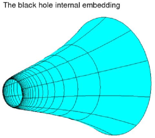
Figure 15: An embedding of the spacetime inside a black hole. The singularity is to the left and the horizon is to the right. Schwarzschild time is still the azimuthal angle.

The trumpet is now narrowing towards the singularity, implying acceleration away from the singularity in the sense that a geodesic that was at some point, moving solely in Schwarzschild time, will end up at the horizon. Inside the horizon however, moving only in $t$, means moving faster than light. Thus it is tachyons (time-lines) that accelerate out towards the horizon.

Real observers are however always approaching the singularity. While we might find it unintuitive that the shape of the trumpet implies that they decelerate as they move inwards one must consider also the spacing between lines of constant $x$. If the distance between $x$-lines is decreasing as we approach the horizon, we see that it is quite possible to have increasing $dx/dt$ the closer to the singularity that we are, in spite of the trumpet opening up in the “wrong” direction.

9 Comments on the two-dimensional analysis

The dual metric assigns distances between nearby points on the manifold. This is what metrics in general do. Under a coordinate transformation the dual metric will thus transform as a tensor.

If we make a coordinate transformation to some wobbling coordinates, the dual metric will appear complicated. However, when we embed it we get the static-looking spacetime depicted in Fig. 11. It’s like the ugly duckling becoming a swan. The difference is that the coordinate lines will now wind and twist on the surface. Notice however that while the embedding of the dual metric is coordinate independent there may in principle exist more ways of embedding it than as a rotational surface.

We understand that if the dual metric exists in one coordinate system it exists in all coordinate systems. In particular this means that it is sufficient that there exists coordinates where $a$ and $c$ are time independent, for the dual metric to exist. Also we realize that, starting from the Schwarzschild line element, written in standard coordinates, we are not excluding any possible dual metrics through our choice of coordinates. However we may be excluding dual metrics by our assumption that the dual metric is time independent and diagonal.

Another small comment. One may think that the dual metric and the original metric would have the same affine connection, since the affine connection is all that enters the geodesic equation:

$$\frac{d^{2}x^{\lambda}}{d\tau^{2}}+\Gamma^{\lambda}_{\mu\nu}\frac{dx^{\mu}}{d\tau}\frac{dx^{\nu}}{d\tau}=0$$ (53)

Explicitly calculating the dual and original affine connections we find however that they are not the same. The explanation is that in the geodesic equation there are derivatives with respect to proper distance (eigentime). When we change into the dual metric we change the meaning, in a nontrivial way, of the proper distance. Then we see the possibility that different affine connections can produce the same $x(t)$.

A final comment is in order. The dual metric of Eq. (10) and Eq. (11) is Riemannian from infinity and in to the point where $\beta=a_{0}$. It is however geodesically equivalent to the original Schwarzschild metric also inside this boundary. Here $a$ is negative while $c$ is still positive (until we reach the real horizon where they both flip sign) implying a Lorentzian signature. This signature boundary has nothing to do with coordinates. Coordinate choices will not affect whether there exists negative distances or not. While we can not embed the Lorentzian part, it is however interesting to see that we can have smooth geodesics moving over something as dramatic as a signature change.

10 Extension to 2+1-dimensional spacetimes

I have extended the dual metric analysis to higher dimensions, using techniques very similar to those used in the 1+1-dimensional case. Assuming both the original and the dual metric to be time independent and diagonal, I find that there is in general no dual positive definite metric. The problem is that one needs the extra metrical function (connected to azimuthal distance) to fix $x(t)$ for all values of the angular momentum $J_{0}$, but one also needs the extra metrical component to get the azimuthal motion right. It’s simply over-determined.

Only for very specific cases of original metrics can we find a dual metric that is positive definite. In particular assuming the original metric to have $g_{tt}=\textrm{const}$, we find the dual metric simply by flipping the sign of the spatial part. This may be understood without any analysis at all.

However, if we restrict ourselves to demand that only those geodesics that correspond to a certain energy ($K$), shall be geodesics in the new metric – we can find a nontrivial dual metric. In particular studying photons, that have infinite $K$, the equations for the dual metric are somewhat simplified:

$$a = \frac{\lambda-1}{k_{3}\frac{d_{0}}{a_{0}}-k_{2}}$$ (54)

$$c = \frac{c_{0}}{a_{0}}\cdot a(1-k_{2}a)$$ (55)

$$d = \lambda\cdot\frac{d_{0}}{a_{0}}\cdot a$$ (56)

Here, $k_{3}$, $k_{2}$ and $\lambda$ are gauge constants much like $\alpha$ and $\beta$ in the two-dimensional analysis. Consider an original metric of the form:

$$d\tau^{2}=a_{0}\cdot dt^{2}+c_{0}\cdot dx^{2}-x^{2}\cdot d\theta^{2}$$ (57)

Let us assume that $a_{0}$ and $c_{0}$ reduces to +1 and -1 respectively at infinity. Demanding the dual metric to be flat Euclidean space expressed in polar coordinates at infinity, i.e. $a=1$, $c=1$ and $d=x^{2}$, yields $k_{3}=0$, $k_{2}=2$ and $\lambda=-1$. Inserting these constants into Eq. (54)-Eq. (56) gives:

$$a=1\qquad\qquad c=\frac{-c_{0}}{a_{0}}\qquad\qquad d=\frac{x^{2}}{a_{0}}$$ (58)

This is thus a metric with positive signature that is geodesically dual to the original metric with respect to photons. The spatial part we recognize as the optical geometry, see [4]. For a brief review applicable to this text see Appendix A.

When $a$ is constant it is easy to understand that geodesics in spacetime are also geodesics in space. We may thus embed the spatial part of the dual metric to visualize a space where photons move on the shortest path. See Fig. 16.

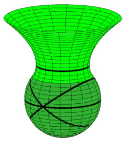
Figure 16: The optical geometry of a plane through a star with $x_{0}=1.2$. The great circles are closed photon orbits within the star.

It is a little bit fascinating that asking for a metric that is geodesically dual with respect to photons, with positive signature, yields the optical geometry, which is normally derived in a completely different manner.

Notice however that we knew in advance that the optical geometry (plus time) would be among the possible dual spacetimes. We knew that there existed a three-metric (essentially Fig. 16) for Schwarzschild in which photons moved on geodesics. To this space we knew that we could just add time to create a Riemannian spacetime in which photons would move on geodesics. Thus we knew that the optical geometry (plus time) would be among the possible solutions. It turned out to be the only dual spacetime that reduced to a Euclidean spacetime at infinity.

One may also study the dual geometry that springs from other choices of $K$, but then $a$ doesn’t become constant and the geometrical information doesn’t lie entirely in a spatial metric.

Still it is interesting to see that we have a scheme that produces the optical geometry for the particular case of photons. What would be really nice would be if we, using insights and techniques developed in this paper, could generalize the optical geometry to something that makes sense even when the spacetime is not conformally static.

10.1 Comments on the higher dimension analysis

If we introduce freedoms, like off-diagonality and time dependence, it may after all be possible to find a dual metric in higher dimensions. For me it is therefore still an open question whether, as soon as we have a fairly nontrivial metric, we can decide the exact form of the metric up to a global rescaling constant by just studying geodesics? In the two-dimensional analysis it was not so, but in the three-dimensional analysis it was so, assuming time independence and diagonality of the dual metric. In general however I do not know yet.

11 Comparison to other works

In Lewis Carrol Epstein’s book ’Relativity visualized’ [2], there is a similar way of visualizing the acceleration towards a gravitational source. The pictures illustrated are qualitatively very similar to my own, a star is a bulge on a cylinder for instance. In Epstein’s view however the azimuthal angle on the rotational surface is the eigentime experienced by an observer (for instance a freefaller). The Euclidean length of a curve on the surface is the Schwarzschild time elapsed. All freefallers move on geodesics on the surface. In particular photons, which do not experience eigentime, but still travels in Schwarzschild time, are represented by straight lines directed along the rotational surface, without the slightest spiral in the azimuthal direction.

The Epstein view is very beautiful in many respects. For instance it naturally explains why it takes infinite Schwarzschild time to reach the horizon but only finite eigentime. What Epstein is embedding is however not strictly a spacetime. A point on his surface is not corresponding to a unique event (in general). To see this consider a photon moving in towards the gravitational source and then bouncing back outwards. In the Epstein diagram the photon returns to the same point that it came from. Thus one point in the Epstein diagram represents two events (at least!) in the physical world. Also in the Epstein view one can not display spacelike distances.

Perhaps the biggest advantage of my view, compared to Epstein’s view, is the opportunity to graphically display how gravity on Earth can be explained by spacetime geometry. This is obviously difficult to accomplish with the Epstein view since eigentime and Schwarzschild time are virtually the same thing for us Earthlings.

We understand that the two approaches complement each other. It is really fascinating however that two such fundamentally different approaches can produce more or less the same plots!

Another way of illustrating curved spacetime is to embed the spacetime in a 2+1 Minkowski space. There one has access to null and negative distances. See the paper [1], by Donald Marolf. The beauty of this scheme is that one can deduce Lorentzian distances between points just from the slope of the surface. Also particles move on geodesics, in the sense of shortest Euclidean distance on the surface. These surfaces are not rotational surfaces (in general), and depend on the timelike parameter.

In particular Marolf studies the embedding of a Kruskal spacetime of an eternal black hole. The horizons are included in the embedding but not the singularities and the infinities. A lot of physics can be displayed in this type of embedding. For instance one can illustrate how tidal forces become infinite as one approaches the singularity. Fascinating.

12 Summary

Always for a two-dimensional time independent diagonal original metric with $a_{0}$ positive and $c_{0}$ negative we can find a dual metric where both $a$ and $c$ are positive. The new dual metric is dual in the sense that it produces the same geodesics as the original metric.

$$a = \alpha\cdot\frac{a_{0}}{a_{0}-\beta}\qquad\qquad\qquad 0<\beta<\textrm{min}\{a_{0}\}\qquad\qquad 0<\alpha$$ (59)

$$c = \alpha\cdot\frac{-c_{0}\beta}{\left(a_{0}-\beta\right)^{2}}$$ (60)

Here $\alpha$ and $\beta$ are gauge freedoms in the dual metric. $\alpha$ is an overall rescaling. $\beta$ is connected to stretching in the $x$-direction, while it can also be considered as a rescaling of the original metric. In particular, starting from the exterior Schwarzschild metric, and demanding that the dual metric reduces to Pythagoras at infinity yields $\alpha=\frac{1}{2}$ and $\beta=\frac{1}{2}$, the standard gauge. The dual line element may then be written:

$$ds^{2} = \frac{x-1}{x-2}\cdot dt^{2}+\frac{x^{3}}{(x-1)(x-2)^{2}}\cdot dx^{2}$$ (61)

In this particular gauge the dual metric stays Riemannian from infinity and in to $x=2$. By choosing other gauge constants we can move this boundary arbitrarily close to the horizon.

We may embed the dual metric as a rotational surface in Euclidean space. We have then an embedding freedom $k$. Increasing $k$ means increasing the radius and the slope of the rotational surface everywhere.

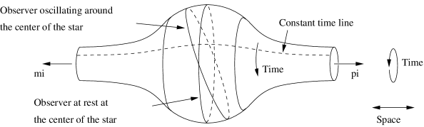
Figure 17: The spacetime of a central line through a star.

A schematic embedding of the dual metric of a radial line through a star is depicted in Fig. 17. The spacetime surface is layered, so walking around the rotational body one lap means that you come to a new spacetime point. Azimuthal angle on the surface is proportional to the Schwarzschild time.

• For non-compact stars, using the standard gauge and $k=1$, the difference between the radius of the rotational surface and the radius at infinity, is proportional to minus the Newtonian potential.

• We have all in all three parameters, $\alpha$, $\beta$ and $k$, that affects the shape and size of the embedding diagram. In particular this allows us to visualize, with substantial curvature, why, and how fast, our keys fall when we drop them in our office.

• The dual metric is geodesically equivalent to the original also in regions where $a_{0}<\beta$. Here it has Lorentzian signature however.

• We can embed (parts of) the inside of a Schwarzschild black hole simply by putting $\beta$ negative in Eq. (59) and Eq. (60).

• In 2+1 dimensions we can not generally find a dual metric that is diagonal and time independent. We can however relax the constraints on the dual metric to apply, not to all geodesics, but only photon geodesics. That way we can re-derive the optical geometry.

It would be interesting to generalize the dual metric scheme, to include more general original and dual metrics. In particular it would be interesting to study an equatorial plane in a Kerr geometry, and restrict ourselves to photons. Also, using the dual metric scheme, it remains to be seen if we can somehow include the horizon in the embedding, maybe using just a certain set of observers.

13 Conclusions

The ideas presented in this article are probably of minor practical use in calculations and the finding of new physics. Nevertheless they are, I think, of great pedagogical value. They open up our minds to possibilities that we might not have considered earlier. This goes for both professionals in the field, but even more so for those who have never seen a $g_{\mu\nu}$, or even an $\eta_{\mu\nu}$.

For the experts it is probably the concept of the geodesically dual metric itself that is most interesting. The signature change in the dual metric may as well attract some attention. Also it was nice, though not surprising, to see the optical geometry coming naturally from relaxing the geodesic demands to apply only to photons.

For the non-experts it is probably Fig. 14, depicting the spacetime at the surface of the Earth, that has the greatest pedagogical value. Especially useful would it be to construct such a surface, with meter lines and second lines, and threads to pull tight between various spacetime points. Then people get a chance to see how acceleration can be explained by geometry. This I think is very powerful, and something that I have longed for, when giving introductory lectures on general relativity.

Appendix A Review of the optical geometry

Null geodesics are conserved under conformal rescalings of the metric. If we have a manifestly time independent metric, with no cross-terms of $dt$ (e.g. Schwarzschild), we may rescale it by $g_{tt}^{-1}(x^{\mu})$ without affecting the null geodesics. The rescaled metric will consist of a unit time-time component, and a spatial three-metric. It is thus a curved space, with time. There is no acceleration or time dilation. For such a metric, a so called ultrastatic metric, it is easy to understand that geodesics in spacetime are also geodesics in space.

So, by rescaling the spatial part of, for instance Schwarzschild, with $g_{tt}^{-1}$ we create a space in which photons moves on geodesics. This rescaled space is known as the optical space.

References

- [1] Marolf, D. (1999). Gen. Rel. Grav. 31, 919
- [2] Epstein, L. C. (1994). Relativity Visualized, (Insight Press, San Fransisco), ch. 10,11,12
- [3] Weinberg, S. (1972). Gravitation and Cosmology: Principles and Applications of the General Theory of Relativity, (John Wiley & Sons, U.S.A), p. 77
- [4] Kristiansson, S., Sonego, S., and Abramowicz, M. A. (1998). Gen. Rel. Grav. 30, 275
- [5] D’Inverno, R. (1998). Introducing Einstein’s Relativity, (Oxford University Press, Oxford), p. 99-101