Online Learning in Discrete Hidden Markov Models

Abstract

We present and analyse three online algorithms for learning in discrete Hidden Markov Models (HMMs) and compare them with the Baldi-Chauvin Algorithm. Using the Kullback-Leibler divergence as a measure of generalisation error we draw learning curves in simplified situations. The performance for learning drifting concepts of one of the presented algorithms is analysed and compared with the Baldi-Chauvin algorithm in the same situations. A brief discussion about learning and symmetry breaking based on our results is also presented.
 
Key Words: HMMs, Online Algorithm, Generalisation Error, Bayesian Algorithm.

1 Introduction

Hidden Markov Models (HMMs) Ephraim02 ; Rabiner89 are extensively studied machine learning models for time series with several applications in fields like speech recognition Rabiner89 , bioinformatics Baldi01 ; Durbin98 and LDPC codes Frias04 . They consist of a Markov chain of non-observable hidden states $q_{t}\in S$, $t=1,...,T$, $S=\{s_{1},s_{2},...,s_{n}\}$, with initial probability vector $\pi_{i}=\mathcal{P}(q_{1}=s_{i})$ and transition matrix $A_{ij}(t)=\mathcal{P}(q_{t+1}=s_{j}|q_{t}=s_{i})$, $i,j=1,..,n$. At discrete times $t$, each $q_{t}$ emits an observed state $y_{t}\in O$, $O=\{o_{1},...,o_{m}\}$, with emission probability matrix $B_{i\alpha}(t)=\mathcal{P}(y_{t}=o_{\alpha}|q_{t}=s_{i})$, $i=1,...,n$, $\alpha=1,...,m$, which are the actual observations of the time series represented, from time $t=1$ to $t=T$, by the observed sequence $y_{1}^{T}=\{y_{1},y_{2},...,y_{T}\}$. The $q_{t}$’s form the so called hidden sequence $q_{1}^{T}=\{q_{1},q_{2},...,q_{T}\}$. The probability of observing a sequence $y_{1}^{T}$ given $\omega\equiv(\pi,A,B)$ is

$$\mathcal{P}(y_{1}^{T}|\omega)=\sum_{q_{1}^{T}}\mathcal{P}(y_{1})\mathcal{P}(y_{1}|q_{1})\prod_{t=2}^{T}\mathcal{P}(q_{t+1}|q_{t})\mathcal{P}(y_{t}|q_{t}).$$ (1)

In the learning process, the HMM is fed with a series and adapts its parameters to produce similar ones. Data feeding can range from offline (all data is fed and parameters calculated all at once) to online (data is fed by parts and partial calculations are made).

We study a scenario with data generated by a HMM of unknown parameters, an extension of the student-teacher scenario from neural networks. The performance, as a function of the number of observations, is given by how far, measured by a suitable criterion, is the student from the teacher. Here we use the naturally arising Kullback-Leibler (KL) divergence that, although not accessible in practice since it needs knowledge of the teacher, is an extension of the idea of generalisation error being very informative.

We propose three algorithms and compare them with the Baldi-Chauvin Algorithm (BC) Baldi94 : the Baum-Welch Online Algorithm (BWO), an adaptation of the offline Baum-Welch Reestimation Formulas (BW) Ephraim02 and, starting from a Bayesian formulation, an approximation named Bayesian Online Algorithm (BOnA), that can be simplified again without noticeable lost of performance to a Mean Posterior Algorithm (MPA). BOnA and MPA, inspired by Amari Amari and Opper Opper98 , are essentially mean field methods Saad in which a manifold of prior tractable distributions is introduced and the new datum leads, through Bayes theorem, to a non-tractable posterior. The key step is to take as the new prior, not the posterior, but the closest distribution (in some sense) in the manifold.

The paper is organised as follows: first, BWO is introduced and analysed. Next, we derive BOnA for HMMs and, from it, MPA. We compare MPA and BC for drifting concepts. Then, we discuss learning and symmetry breaking and end with our conclusions.

2 Baum-Welch Online Algorithm

The Baum-Welch Online Algorithm (BWO) is an online adaptation of BW where in each iteration of BW, $y$ becomes $y^{p}$, the $p$-th observed sequence. Multiplying the BW increment by a learning rate $\eta_{BW}$ we get the update equations for $\omega$

$$\hat{\omega}^{p+1}=\hat{\omega}^{p}+\eta_{BW}\hat{\Delta}\omega^{p},$$ (2)

with $\hat{\Delta}\omega^{p}$ the BW variations for $y^{p}$. The complexity of BWO is polynomial in $n$ and $T$.

In figure 1, the HMM learns sequences generated by a teacher with $n=2$, $m=3$ and $T=2$ for different $\eta_{BW}$. Initial students have matrices with all entries set to the same value, what we call a symmetric initial student. We took averages over 500 random teachers and distances are given by the KL-divergence between two HMMs $\omega_{1}$ and $\omega_{2}$

$$d_{KL}(\omega_{1},\omega_{2})\equiv\sum_{y_{1}^{T}}\mathcal{P}(y_{1}^{T}|\omega_{1})\ln\left[\frac{\mathcal{P}(y_{1}^{T}|\omega_{1})}{\mathcal{P}(y_{1}^{T}|\omega_{2})}\right].$$ (3)

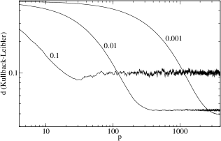
Figure 1: Log-log curves of BWO for three different $\eta_{BW}$ indicated next to the curves.

We see that after a certain number of sequences the HMM stops learning, which is particular to the symmetric initial student and disappears for a non-symmetric one.

Denoting the variation of the parameters in BC by $\Delta$, in BW by $\hat{\Delta}$, in BWO by $\tilde{\Delta}$, and with $\gamma_{t}(i)\equiv\mathcal{P}(q_{t}=s_{i}|y^{p},\omega^{p})$, we have to first order in $\lambda$

$$\Delta\pi_{i} = \frac{\lambda\eta_{BC}}{n}\hat{\Delta}\pi_{i}=\frac{\lambda}{n}\frac{\eta_{BC}}{\eta_{BW}}\tilde{\Delta}\pi_{i},$$ (4)

$$\Delta A_{ij} = \frac{\lambda\eta_{BC}}{n}\left[\sum_{t=1}^{T-1}\gamma_{t}(i)\right]\hat{\Delta}A_{ij}=\frac{\lambda}{n}\frac{\eta_{BC}}{\eta_{BW}}\left[\sum_{t=1}^{T-1}\gamma_{t}(i)\right]\tilde{\Delta}A_{ij},$$

$$\Delta B_{i\alpha} = \frac{\lambda\eta_{BC}}{n}\left[\sum_{t=1}^{T}\gamma_{t}(i)\right]\hat{\Delta}B_{i\alpha}=\frac{\lambda}{n}\frac{\eta_{BC}}{\eta_{BW}}\left[\sum_{t=1}^{T}\gamma_{t}(i)\right]\tilde{\Delta}B_{i\alpha}.$$

For $\eta_{BW}\approx\lambda\eta_{BC}/n$ and small $\lambda$, variations in BC are proportional to those in BWO, but with different effective learning rates for each matrix depending on $y^{p}$. Simulations show that actual values are of the same order of approximated ones.

3 The Bayesian Online Algorithm

The Bayesian Online Algorithm (BOnA) Opper98 uses Bayesian inference to adjust $\omega$ in the HMM using a data set $D_{P}=\{y^{1},...,y^{P}\}$. For each data, the prior distribution is updated by Bayes’ theorem. This update takes a prior from a parametric family and transforms it in a posterior which in general has no longer the same parametric form. The strategy used by BOnA is then to project the posterior back into the initial parametric family. In order to achieve this, we minimise the KL-divergence between the posterior and a distribution in the parametric family. This minimisation will enable us to find the parameters of the closest parametric distribution by which we will approximate our posterior. The student HMM $\omega$ parameters in each step of the learning process are estimated as the means of the each projected distribution.

For a parametric family that has the form $P(x)\propto e^{-\sum_{i}\lambda_{i}f_{i}(x)}$, which can be obtained by the MaxEnt principle where we constrain the averages over $P(x)$ of arbitrary functions $f_{i}(x)$, minimising the KL-divergence turns out to be equivalent to equating the averages $<f_{i}(x)>$ over $P(x)$ to the average of these functions over the unprojected posterior (our posterior distribution just after the Bayesian update for the next data).

For HMMs, the vector $\pi$ and each $i$-th row $A^{i}$ of $A$ and $B^{i}$ of $B$ are different discrete distributions which we assume independent in order to write the factorized distribution

$$\mathcal{P}(\omega|u)\equiv\mathcal{P}(\pi|\rho)\prod_{i=1}^{n}\mathcal{P}(A^{i}|a^{i})\mathcal{P}(B^{i}|b^{i}),$$ (5)

where $u=(\rho,a,b)$ represents the parameters of the distributions.

As each factor is a distribution over probabilities, the natural choice are the Dirichlet distributions, which for a $N$-dimensional variable $x$ is

$$\mathcal{D}(x|u)=\frac{\Gamma(u_{0})}{\prod_{i=1}^{N}\Gamma(u_{i})}\prod_{i=1}^{N}x_{i}^{u_{i}-1},$$ (6)

where $u_{0}=\sum_{i}u_{i}$ and $\Gamma$ is the analytical continuation of the factorial to real numbers. These can be obtained from MaxEnt with $f_{i}(x)=\ln x_{i}$ Vlad :

$$\int d\mu\,\mathcal{D}(x)\ln x_{i}=\alpha_{i},\qquad d\mu\equiv\delta\left(\sum_{i}x_{i}-1\right)\prod_{i}\theta(x_{i})dx_{i}.$$ (7)

The function to be extremized is

$$\mathcal{L}=\int d\mu\,\mathcal{D}\ln\mathcal{D}+\lambda\left(\int d\mu\,\mathcal{D}-1\right)+\sum_{i}\lambda_{i}\left(\int d\mu\,\mathcal{D}\ln x_{i}-\alpha_{i}\right),$$ (8)

and with $\delta\mathcal{L}/\delta\mathcal{D}=0$ we get the Dirichlet with normalisation $e^{\lambda+1}$ and $u_{i}=1-\lambda_{i}$.

Each factor distribution is separately projected by equating the average of the logarithms in the original posterior $Q$ and in the projected distributions

$$\psi(\rho_{i})-\psi\left(\sum_{j}\rho_{j}\right) = \left<\ln\pi_{i}\right>_{Q}\equiv\mu_{i}(\rho),$$ (9)

$$\psi(a_{ij})-\psi\left(\sum_{k}a_{ik}\right) = \left<\ln A_{ij}\right>_{Q}\equiv\mu_{ij}(a),$$

$$\psi(b_{i\alpha})-\psi\left(\sum_{\beta}b_{i\beta}\right) = \left<\ln B_{i\alpha}\right>_{Q}\equiv\mu_{i\alpha}(b),$$

where $\psi(x)=d\ln\Gamma(x)/dx$ is the digamma function. We call a set of $N$ equations

$$\psi(x_{i})-\psi\left(\sum_{j}x_{j}\right)=\mu_{i},\\$$ (10)

with $i=1,...N$ a digamma system in the variables $x_{i}$ with coefficients $\mu_{i}$.

Let us call $P^{p}(\omega)$ the projected distribution after observation of $y^{p}$, and $Q^{p+1}(\omega)$ the posterior distribution (not projected yet) after $y^{p+1}$. By Bayes’ theorem,

$$Q^{p+1}(\omega)\propto P^{p}(\omega)\sum_{q^{p+1}}\mathcal{P}(y^{p+1},q^{p+1}|\omega).$$ (11)

The calculation of $\mu$’s in (9) leads to averages over Dirichlets of the form Alamino

$$\mu_{i}=\left<\left[\prod_{j}x_{j}^{r_{j}}\right]\ln x_{i}\right>=\frac{\Gamma(u_{0})}{\prod_{j}\Gamma(u_{j})}\frac{\prod_{j}\Gamma(u_{j}+r_{j})}{\Gamma(u_{0}+r_{0})}[\psi(u_{i}+r_{i})-\psi(u_{0}+r_{0})].$$ (12)

To solve (10), we solve for $x_{i}$, sum over $i$ with $x_{0}\equiv\sum_{i}x_{i}$ and find numerically, by iterating from an arbitrary initial point, the fixed points of the one-dimensional map

$$x_{0}^{n+1}=\sum_{i}\psi^{-1}[\mu_{i}+\psi(x_{0}^{n})],$$ (13)

where we found a unique solution except for $\mu_{i}\approx 0$, which is rare in most applications.

BOnA has a common problem of Bayesian algorithms: the sum over hidden variables makes the complexity scales exponentially in $T$. Also, the calculation of several digamma functions is very time consuming. In the following, we develop an approximation that runs faster, although still with exponential complexity in $T$. This is not a problem for we can make $T$ constant and the algorithm will scale polynomially in $n$.

4 Mean Posterior Approximation

The Mean Posterior Approximation (MPA) is a simplification of BOnA inspired in its results for Gaussians, where we match first and second moments of posterior and projected distributions. Noting it, instead of minimising $d_{KL}$ we match the mean and one of the variances of posterior and projected distributions as an approximation, which gives, with hatted variables for reestimated values Alamino

$$\hat{\rho}_{i} = \left<\pi_{i}\right>_{Q}\frac{\left<\pi_{1}\right>_{Q}-\left<\pi_{1}^{2}\right>_{Q}}{\left<\pi_{1}^{2}\right>_{Q}-\left<\pi_{1}\right>_{Q}^{2}},$$ (14)

$$\hat{a}_{ij} = \left<a_{ij}\right>_{Q}\frac{\left<a_{i1}\right>_{Q}-\left<a_{i1}^{2}\right>_{Q}}{\left<a_{i1}^{2}\right>_{Q}-\left<a_{i1}\right>_{Q}^{2}},$$

$$\hat{b}_{i\alpha} = \left<b_{i\alpha}\right>_{Q}\frac{\left<b_{i1}\right>_{Q}-\left<b_{i1}^{2}\right>_{Q}}{\left<b_{i1}^{2}\right>_{Q}-\left<b_{i1}\right>_{Q}^{2}},$$

with complexity again of order $n^{T}$, but with heavily reduced real computational time making it better for practical applications.

Figure 2 compares MPA and BOnA. The initial difference decreases in time and both come closer relatively fast. We used $n=2$, $m=3$ and $T=2$ and averaged over 150 random teachers with symmetric initial students. The computational time for BOnA was 340min, and for MPA, 5s in a 1GHz processor. Figure 3a compares MPA to BC and figure 3b to BWO. In both cases MPA has better generalisation. We used $n=2$, $m=3$, $T=2$, symmetric initial students and averaged over 500 random teachers.

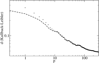
Figure 2: Comparison in log-log scale of MPA (dashed line) and BOnA (circles).

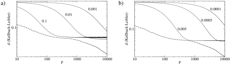
Figure 3: a) Comparison between MPA (dashed) and BC (continuous). Values of $\lambda$ are indicated next to the curves. $\eta_{BC}=0.5$. b) Comparison between MPA (dashed) and BWO (continuous). Values of $\eta_{BW}$ are indicated next to the curves. Both scales are log-log.

5 Learning Drifting Concepts

We tested BC and MPA for changing teachers. In figure 4a, it changes at random after each 500 sequences ($\lambda=0.01$, $\eta_{BC}=10.0$). In figure 4b, each time a sequence is observed, a small random quantity is added to the teacher. Both have $n=2$, $m=3$ and are averaged over 200 runs.

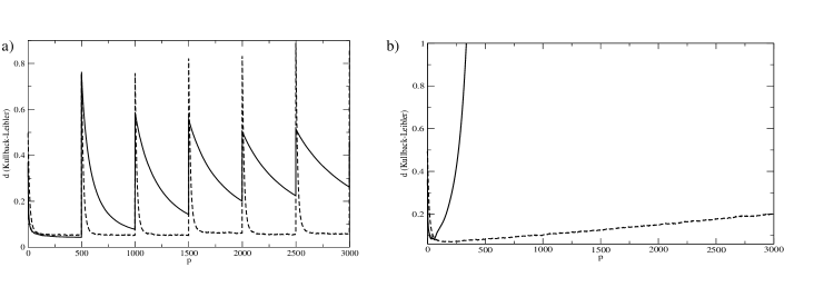
Figure 4: Drifting concepts. Continuous lines correspond to MPA and dashed lines to BC. a) Abrupt changes at 500 sequences interval. b) Small random changes at each new sequence.

Figure 4b shows that BC adapts better, but is not fully adaptive and we do not know how to modify it. MPA instead derives from Bayesian principles and we can guess the problem by analogy with similar Bayesian algorithms Vicente : variances decrease in the process as in the perceptron, where they are the learning rates, explaining the memory effect difficulting the learning after changes. Although not proved yet, we expect the same relationship in MPA, which can be used to improve performance.

6 Learning and Symmetry Breaking

Learning from symmetric initial students requires that the parameters separate from each other in some point, which depends on the algorithm and is an important feature in online algorithms Heskes , breaking the symmetry with a sharp decrease in the generalisation error.

Instead of taking averages to smooth abrupt changes, here we draw curves for only one teacher, rendering them visible. Flat lines before a symmetry breaking are called plateaux and occur when it is difficult to break the symmetry.

Figure 5a shows BC ($\lambda=0.01$, $\eta_{BC}=1.0$) with two abrupt changes: in the beginning and after 1000 sequences. $\pi$ and $A$ only break the symmetry in the second point, and $B$ in both. Figure 5b shows that in MPA the second change is stronger and the symmetry breaking affects both $B$ and $A$. Figure 6 shows BWO with $\eta_{BW}=0.01$ where only $B$ is affected. The more symmetries are broken, the best the generalisation of the algorithm.

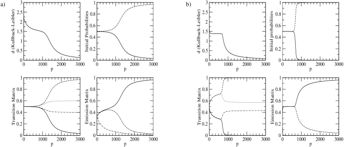
Figure 5: KL-divergence and student’s parameters for a) BC and b) MPA.

In all simulations we set $n=2$, $m=3$ and $T=2$ with a teacher HMM given by

$$\pi=\left(\begin{array}[]{c}1\\ 0\end{array}\right),\qquad A=\left(\begin{array}[]{cc}0&1\\ 1&0\end{array}\right),\qquad B=\left(\begin{array}[]{ccc}1&0&0\\ 0&0&1\end{array}\right).$$ (15)

7 Conclusions

We proposed and analysed three learning algorithms for HMMs: Baum-Welch Online (BWO), Bayesian Online Algorithm (BOnA) and Mean Posterior Approximation (MPA). We showed the superior performance of MPA for static teachers, but the Baldi-Chauvin (BC) algorithm is better for drifting concepts, although the Bayesian nature of MPA suggests how to fix it. The results seem to be confirmed by initial tests on real data.

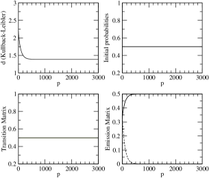
Figure 6: KL-divergence and student’s parameters for BWO.

The importance of symmetry breaking in learning processes is presented here in a brief discussion where the phenomenon is shown to occur in our models.

8 Acknowledgements

We would like to thank Evaldo Oliveira, Manfred Opper and Lehel Csato for useful discussions. This work was made part in the University of São Paulo with financial support of FAPESP and part in the Aston University with support of Evergrow Project.

References

- (1) Y. Ephraim, N. Merhav, Hidden Markov Processes. IEEE Trans. Inf. Theory 48, 1518-1569 (2002).
- (2) L. R. Rabiner, A Tutorial on Hidden Markov Models and Selected Applications in Speech Recognition. Proc. IEEE 77, 257-286 (1989).
- (3) P. Baldi, S. Brunak, Bioinformatics: The Machine Learning Approach. MIT Press (2001).
- (4) R. Durbin, S. Eddy, A. Krogh, G. Mitchison, Biological sequence analysis: Probabilistic models of proteins and nucleic acids. Cambridge University Press, Cambridge (1998).
- (5) J. Garcia-Frias, Decoding of Low-Density Parity-Check Codes Over Finite-State Binary Markov Channels. IEEE Trans. Comm. 52, 1840-1843 (2004).
- (6) P. Baldi, Y. Chauvin, Smooth On-Line Learning Algorithms for Hidden Markov Models. Neural Computation 6, 307-318 (1994).
- (7) S. Amari, Neural learning in structured parameter spaces - Natural Riemannian gradient. NIPS’96 9, MIT Press (1996).
- (8) M. Opper, A Bayesian Approach to On-line Learning. On-line learning in Neural Networks, edited by D. Saad, Publications of the Newton Institute, Cambridge Press, Cambridge (1998).
- (9) M. Opper, D. Saad, Advanced Mean Field Methods: Theory and Practice. MIT Press (2001).
- (10) R. Alamino, N. Caticha, Bayesian Online Algorithms for Learning in Discrete Hidden Markov Models. Submitted to Discrete and Continuous Dynamical Systems.
- (11) T. Heskes, W. Wiegerinck, W., On-line Learning with Time-Correlated Examples. On-line Learning in Neural Networks, 251-278, edited by David Saad, Cambridge University Press, Cambridge (1998).
- (12) R. Vicente, O. Kinouchi, N. Caticha. Statistical Mechanics of Online Learning of Drifting Concepts: A Variational Approach. Machine Learning 32, 179-201 (1998).
- (13) M. O. Vlad, M. Tsuchiya, P. Oefner, J. Ross. Bayesian analysis of systems with random chemical composition: Renormalization-group approach to Dirichlet distributions and the statistical theory of dilution. Phys. Rev. E 65, 011112(1)-01112(8) (2001).