Magnetic Phase Diagram of Spin-1/2 Two-Leg Ladder with Four-Spin Ring Exchange

Abstract

We study the spin-$1/2$ two-leg Heisenberg ladder with four-spin ring exchanges under a magnetic field. We introduce an exact duality transformation which is an extension of the spin-chirality duality developed previously and yields a new self-dual surface in the parameter space. We then determine the magnetic phase diagram using the numerical approaches of the density-matrix renormalization-group and exact diagonalization methods. We demonstrate the appearance of a magnetization plateau and the Tomonaga-Luttinger liquid with dominant vector-chirality quasi-long-range order for a wide parameter regime of strong ring exchange. A “nematic” phase, in which magnons form bound pairs and the magnon-pairing correlation functions dominate, is also identified.

1 Introduction

Multiple-spin ring-exchange process – a process in which several particles with spin permute their positions in a cyclic fashion – has been found to be important in a wide variety of materials. It has been established that ring exchanges are responsible for the magnetism of solid ³He[1, 2] as well as of two-dimensional quantum solids including ³He adsorbed on graphite[3, 4, 5] and Wigner crystals.[2, 6, 7, 8] Ring exchanges were also found to be relevant to some strongly correlated electron systems such as the two-leg spin ladder compound La_xCa_14-xCu₂₄O₄₁[9, 10, 11, 12, 13] and two-dimensional antiferromagnet La₂CuO₄.[14, 15, 16, 17, 18, 19] It has been suggested recently that ring exchanges can be dominant in quantum wires with a shallow confining potential.[20, 21]

In contrast to two- and three-spin exchange processes, the ring exchanges involving more than three spins take a very complicated form in terms of spin operators including bilinear, biquadratic, and higher-order couplings in general, which compete with each other. The multiple-spin ring exchanges therefore contain strong frustration in themselves and can induce exotic phenomena. Thus motivated, extensive studies have been devoted to clarifying the effects of ring exchanges on quantum spin systems in two-leg ladder,[22, 23, 24, 25, 26, 27, 28] square,[29, 30, 31] and triangular lattices.[32, 33, 34, 35, 36] It has been revealed that the four-spin ring exchange can lead to novel quantum states, e.g., the scalar-chirality ordered state in the two-leg ladder system,[25, 26, 27] the vector-chirality[30] and nematic[31] orderings in the square lattice, and the octapolar order[36] in the triangular lattice.

In this paper, we study the $S=1/2$ two-leg Heisenberg ladder system with four-spin ring exchanges under a magnetic field. The magnetic field lowers the symmetry of the model from SU(2) to U(1), and as a result, opens a possibility of novel quantum states. The model was studied previously by numerical exact-diagonalization method and perturbation theory and it was predicted that the model exhibited a plateau in the magnetization curve[37, 38] and a field-induced incommensurate quasi long-range order (LRO) around the plateau.[39] Further, it was also suggested very recently that the interplay between four-spin exchanges and the magnetic field might give rise to a true LRO of vector chirality.[40] Nevertheless, these studies were limited to antiferromagnetic bilinear couplings and rather weak ring exchange, and therefore, the properties of the model for the regime of strong ring exchange and/or of ferromagnetic bilinear coupling remain unclear.

The aim of the paper is to investigate the ground-state properties of the ladder system with four-spin ring exchanges for the whole parameter space of both the antiferromagnetic and ferromagnetic bilinear exchanges and a finite magnetic field. We first employ a theoretical approach using duality transformations. The so-called spin-chirality duality transformation[26, 27] has proven to be a powerful tool to study the ladder system with four-spin exchanges. We further introduce another duality transformation, which is a simple extension of the spin-chirality duality but gives a nontrivial duality mapping on coupling constants in the Hamiltonian as well as on various order parameters. In particular, applying the latter transformation to the ladder with the ring exchange yields a new self-dual line, which divides the parameter region of strong ring exchange from that of strong ferromagnetic bilinear exchange.

Moreover, we study the system using numerical approaches of the density-matrix renormalization-group (DMRG) and exact diagonalization methods and determine the magnetic phase diagram. We then directly observe the magnetization plateau appearing for a wide parameter region of strong ring-exchange coupling. We find various critical states with different dominant quasi-LRO: In addition to the critical state with dominant Néel-type-spin quasi-LRO found in usual antiferromagnetic two-leg ladder without ring exchange, the vector-chirality-dominant critical state appears for strong ring exchange. More interestingly, we show that a nematic phase, in which magnons form bound pairs and the magnon-pairing correlations are dominant, emerges in a finite region adjacent to the ferromagnetic phase.

The paper is organized as follows. In Section 2, we introduce the model Hamiltonian and summarize its known properties obtained from previous studies. The duality transformations and their application to the ladder system with four-spin exchanges are discussed in Section 3. Section 4 shows our numerical results on the magnetic phase diagram. The results on the magnetization plateau and the vector-chirality-dominant critical phase appearing in the region of strong ring exchange are respectively presented in Section 4.1 and 4.2. The nematic phase in the regime of strong ferromagnetic bilinear coupling is discussed in Section 4.3. Section 5 contains summary and concluding remarks.

2 Model

We consider the $S=1/2$ Heisenberg spin ladder with four-spin ring-exchanges under a magnetic field. The model Hamiltonian is given by

$$\mathcal{H} = \mathcal{H}_{0}+\mathcal{H}_{h}$$ (1)

$$\mathcal{H}_{0} = J_{\rm rung}\sum_{l}{\bf s}_{1,l}\cdot{\bf s}_{2,l}+J_{\rm leg}\sum_{l}\left({\bf s}_{1,l}\cdot{\bf s}_{1,l+1}+{\bf s}_{2,l}\cdot{\bf s}_{2,l+1}\right)$$ (2)

$$+J_{4}\sum_{l}(P_{l}+P_{l}^{-1})$$

$$\mathcal{H}_{h} = -h\sum_{l}\left(s^{z}_{1,l}+s^{z}_{2,l}\right),$$ (3)

where ${\bf s}_{j,l}$ is a spin-$1/2$ operator at a site on $j$-th leg and $l$-th rung and $J_{\rm rung}$ ($J_{\rm leg}$) denotes the bilinear exchange constant on rungs (legs). The operator $P_{l}$ ($P_{l}^{-1}$) represents the four-spin ring-exchange process in which four spins on a plaquette $\{(1,l),(2,l),(2,l+1),(1,l+1)\}$ exchange their positions clockwise (counterclockwise). Throughout this paper, we consider the case of $J_{\rm rung}=J_{\rm leg}=J$ and $J_{4}\geq 0$ and parameterize them as

$$J=\cos\theta,~{}~{}~{}~{}J_{4}=\sin\theta,$$ (4)

where $0\leq\theta\leq\pi$.

In terms of the spin operators, the ring exchange is expressed in a complicated form,

$$P_{l}+P_{l}^{-1} = {\bf s}_{1,l}\cdot{\bf s}_{2,l}+{\bf s}_{1,l+1}\cdot{\bf s}_{2,l+1}+{\bf s}_{1,l}\cdot{\bf s}_{1,l+1}+{\bf s}_{2,l}\cdot{\bf s}_{2,l+1}+{\bf s}_{1,l}\cdot{\bf s}_{2,l+1}+{\bf s}_{2,l}\cdot{\bf s}_{1,l+1}$$ (5)

$$+4({\bf s}_{1,l}\cdot{\bf s}_{2,l})({\bf s}_{1,l+1}\cdot{\bf s}_{2,l+1})+4({\bf s}_{1,l}\cdot{\bf s}_{1,l+1})({\bf s}_{2,l}\cdot{\bf s}_{2,l+1})$$

$$-4({\bf s}_{1,l}\cdot{\bf s}_{2,l+1})({\bf s}_{2,l}\cdot{\bf s}_{1,l+1}),$$

where we omit a constant term. Using this expression, the Hamiltonian (1) is rewritten in a form containing bilinear and biquadratic couplings. For the later use, we introduce an extended Hamiltonian with generalized four-spin exchanges defined as

$$\mathcal{H}_{\rm ext} = J_{\rm r}\sum_{l}{\bf s}_{1,l}\cdot{\bf s}_{2,l}+J_{\rm l}\sum_{l}\left({\bf s}_{1,l}\cdot{\bf s}_{1,l+1}+{\bf s}_{2,l}\cdot{\bf s}_{2,l+1}\right)$$ (6)

$$+J_{\rm d}\sum_{l}\left({\bf s}_{1,l}\cdot{\bf s}_{2,l+1}+{\bf s}_{2,l}\cdot{\bf s}_{1,l+1}\right)$$

$$+J_{\rm rr}\sum_{l}\left({\bf s}_{1,l}\cdot{\bf s}_{2,l}\right)\left({\bf s}_{1,l+1}\cdot{\bf s}_{2,l+1}\right)+J_{\rm ll}\sum_{l}\left({\bf s}_{1,l}\cdot{\bf s}_{1,l+1}\right)\left({\bf s}_{2,l}\cdot{\bf s}_{2,l+1}\right)$$

$$+J_{\rm dd}\sum_{l}\left({\bf s}_{1,l}\cdot{\bf s}_{2,l+1}\right)\left({\bf s}_{2,l}\cdot{\bf s}_{1,l+1}\right)$$

$$-h\sum_{l}\left(s^{z}_{1,l}+s^{z}_{2,l}\right).$$

The ring-exchange model (1) with Eq. (4) is expressed as a parameter line in the extended parameter space, $J_{\rm r}=J+2J_{4}$, $J_{\rm l}=J+J_{4}$, $J_{\rm d}=J_{4}$, and $J_{\rm rr}=J_{\rm ll}=-J_{\rm dd}=4J_{4}$.

The ground-state properties of the ring-exchange model (1) have been studied for some limiting cases. For zero magnetic field $h=0$, the ground-state phase diagram for the whole parameter region was determined by extensive numerical calculations.[25] It was shown that besides the conventional rung-singlet phase ($\theta<0.07\pi$) and ferromagnetic phase ($0.94\pi<\theta$) the model exhibited unconventional phases, including the staggered-dimer phase ($0.07\pi<\theta<0.15\pi$), the scalar-chirality phase ($0.15\pi<\theta<0.39\pi$), and the singlet phases with dominant vector-chirality ($0.39\pi<\theta<0.85\pi$) and collinear-spin ($0.85\pi<\theta<0.94\pi$) short-range orders. All the phases except for the ferromagnetic one have a finite energy gap. Furthermore, the spin-chirality duality transformation,[26, 27] which applies also to the case of $h>0$, revealed various duality relations between order parameters as well as duality mappings in the model Hamiltonian. We will discuss the duality transformation in the following section.

For the antiferromagnetic two-leg spin ladders without ring exchanges, Eq. (1) with $J>0$ and $J_{4}=0$, the effect of the magnetic field has been well understood.[41, 42, 43, 44, 45] The energy gap above the singlet ground state at $h=0$ decreases as the field $h$ increases and closes at a critical field $h_{\rm c}$. The system then enters a critical regime, where the low-energy excitations are described by the one-component Tomonaga-Luttinger (TL) liquid.[41, 43, 44] Throughout the regime, the transverse spin correlation with $(q_{x},q_{y})=(\pi,\pi)$ dominates. The field-dependence of the TL-liquid parameter, which governs the low-energy physics of the system, as well as that of nonuniversal coefficients included in the TL-liquid theory were also obtained numerically.[42, 45] When $h$ exceeds the saturation field $h_{\rm s}$, the fully polarized ground state emerges.

Compared with the cases above, little is known about the case with $J_{4}>0$ and $h>0$. Previous studies were performed for antiferromagnetic bilinear coupling $J>0$ and rather small ring exchange $J_{4}\lesssim J$. From numerical exact-diagonalization studies for small clusters with the level-spectroscopy analysis, it has been shown that for not too small $J_{4}$ a plateau emerges in the magnetization curve at a half of the saturated magnetization.[37, 38] The perturbation theory around the strong-rung-coupling limit $J_{\rm rung}\to\infty$ have concluded that the ground state at the plateau breaks the translational symmetry, resulting in the LRO of the staggered pattern of spin-singlet and spin-triplet rungs. A phenomenon called “$\eta$-inversion”, in which a longitudinal incommensurate spin correlation becomes stronger than the transverse-spin one, was predicted by exact diagonalization, while any direct observation of the behavior of the correlation functions has not been achieved yet.[39] The possibility of the true LRO of vector-chirality was also discussed within the bosonization approach[40] though it is still elusive whether or not it realizes.

3 Duality relations

In this section, we discuss two duality transformations in the extended Hamiltonian $\mathcal{H}_{\rm ext}$ in Eq. (6) and the corresponding duality relations between various phases. The one transformation is the so-called spin-chirality duality and the other is its extension. The former was already introduced and discussed in Refs. HikiharaMH2003 and MomoiHNH2003 in detail, and we present here a brief summary for completeness.

The spin-chirality duality transformation is defined as a mapping from original spin operators in a rung, ${\bf s}_{1,l}$ and ${\bf s}_{2,l}$, into new pseudospin ones; it is given by

$$\tilde{\bf S}_{1,l} \equiv \frac{1}{2}\left({\bf s}_{1,l}+{\bf s}_{2,l}\right)-{\bf s}_{1,l}\times{\bf s}_{2,l},$$

$$\tilde{\bf S}_{2,l} \equiv \frac{1}{2}\left({\bf s}_{1,l}+{\bf s}_{2,l}\right)+{\bf s}_{1,l}\times{\bf s}_{2,l}.$$ (7)

The new pseudospin operators obey the usual commutation relations for spins and satisfy $(\tilde{\bf S}_{1,l})^{2}=(\tilde{\bf S}_{2,l})^{2}=3/4$. The spin-chirality transformation gives duality mappings between various order parameters. For example, the $(q_{x},\pi)$-spin order operator,

$$\mathcal{O}_{\rm s}(q_{x},\pi)=\sum_{l}e^{iq_{x}l}\left({\bf s}_{1,l}-{\bf s}_{2,l}\right),$$ (8)

converts into the vector-chirality one,

$$\tilde{\mathcal{O}}_{\rm vc}(q_{x})=2\sum_{l}e^{iq_{x}l}\tilde{\bf S}_{1,l}\times\tilde{\bf S}_{2,l},$$ (9)

and vise versa (up to an overall sign factor), while the total rung-spin operator ${\bf s}_{1,l}+{\bf s}_{2,l}$ is self-dual under the transformation. We note that the duality transformation (7) corresponds to a unitary transformation,[27]

$$\tilde{\bf S}_{n,l}=U(\{\theta_{l}\}){\bf s}_{n,l}U^{\dagger}(\{\theta_{l}\}),$$ (10)

with a unitary operator,

$$U(\{\theta_{l}\})=\prod_{l}\exp\left[i\theta_{l}\left({\bf s}_{1,l}\cdot{\bf s}_{2,l}-\frac{1}{4}\right)\right],$$ (11)

and $\theta_{l}=\pi/2$ for arbitrary $l$. In this paper, we call this transformation the duality I.

When applied to the extended model $\mathcal{H}_{\rm ext}$, the duality transformation I leaves the form of the Hamiltonian unchanged and gives a duality mapping of the coupling parameters. To see the parameter mapping, it is convenient to rewrite the Hamiltonian as

$$\mathcal{H}_{\rm ext} = J_{\rm r}\sum_{l}{\bf s}_{1,l}\cdot{\bf s}_{2,l}+J_{\rm rr}\sum_{l}\left({\bf s}_{1,l}\cdot{\bf s}_{2,l}\right)\left({\bf s}_{1,l+1}\cdot{\bf s}_{2,l+1}\right)$$ (12)

$$+W\sum_{l}\left({\bf s}_{1,l}+{\bf s}_{2,l}\right)\cdot\left({\bf s}_{1,l+1}+{\bf s}_{2,l+1}\right)$$

$$+X\sum_{l}\left[\left({\bf s}_{1,l}\cdot{\bf s}_{1,l+1}\right)\left({\bf s}_{2,l}\cdot{\bf s}_{2,l+1}\right)+\left({\bf s}_{1,l}\cdot{\bf s}_{2,l+1}\right)\left({\bf s}_{1,l+1}\cdot{\bf s}_{2,l}\right)\right]$$

$$+Y\sum_{l}\left[\left({\bf s}_{1,l}-{\bf s}_{2,l}\right)\cdot\left({\bf s}_{1,l+1}-{\bf s}_{2,l+1}\right)+4\left({\bf s}_{1,l}\times{\bf s}_{2,l}\right)\cdot\left({\bf s}_{1,l+1}\times{\bf s}_{2,l+1}\right)\right]$$

$$+Z\sum_{l}\left[\left({\bf s}_{1,l}-{\bf s}_{2,l}\right)\cdot\left({\bf s}_{1,l+1}-{\bf s}_{2,l+1}\right)-4\left({\bf s}_{1,l}\times{\bf s}_{2,l}\right)\cdot\left({\bf s}_{1,l+1}\times{\bf s}_{2,l+1}\right)\right]$$

$$-h\sum_{l}\left(s^{z}_{1,l}+s^{z}_{2,l}\right),$$

where

$$W = \frac{1}{2}(J_{\rm l}+J_{\rm d}),~{}~{}~{}~{}~{}X=\frac{1}{2}(J_{\rm ll}+J_{\rm dd}),$$

$$Y = \frac{1}{16}(J_{\rm ll}-J_{\rm dd})+\frac{1}{4}(J_{\rm l}-J_{\rm d}),$$

$$Z = -\frac{1}{16}(J_{\rm ll}-J_{\rm dd})+\frac{1}{4}(J_{\rm l}-J_{\rm d}).$$ (13)

After some algebra, one finds that the duality transformation changes the sign of the coupling constant $Z$ to $-Z$ and leaves the other terms unchanged. Therefore, the duality I leads to the mapping in the seven-dimensional parameter space, $(J_{\rm r},J_{\rm rr},W,X,Y,Z,h)$ to $(J_{\rm r},J_{\rm rr},W,X,Y,-Z,h)$. In terms of the original coupling parameters, the mapping is given by

$$\tilde{J}_{\rm r} = J_{\rm r},~{}~{}~{}~{}~{}\tilde{J}_{\rm rr}=J_{\rm rr},$$

$$\tilde{J}_{\rm l} = \frac{1}{2}(J_{\rm l}+J_{\rm d})+\frac{1}{8}(J_{\rm ll}-J_{\rm dd}),~{}~{}~{}~{}~{}\tilde{J}_{\rm d}=\frac{1}{2}(J_{\rm l}+J_{\rm d})-\frac{1}{8}(J_{\rm ll}-J_{\rm dd}),$$

$$\tilde{J}_{\rm ll} = 2(J_{\rm l}-J_{\rm d})+\frac{1}{2}(J_{\rm ll}+J_{\rm dd}),~{}~{}~{}~{}~{}\tilde{J}_{\rm dd}=-2(J_{\rm l}-J_{\rm d})+\frac{1}{2}(J_{\rm ll}+J_{\rm dd}).$$ (14)

The extended model $\mathcal{H}_{\rm ext}$ with $Z=0$, equivalently $4(J_{\rm l}-J_{\rm d})=J_{\rm ll}-J_{\rm dd}$, is therefore self-dual under the duality transformation I.

Since the duality transformation I [Eq. (7) or Eq. (10)] consists of independent transformations within each rung, one can construct arbitrary transformations with any set of the phase factors $\{\theta_{l}\}$. Among them, a set $\{\theta_{l}=(-1)^{l}\pi/2\}$ yields another useful duality transformation given by

$$\bar{\bf S}_{1,l} \equiv \frac{1}{2}\left({\bf s}_{1,l}+{\bf s}_{2,l}\right)-(-1)^{l}{\bf s}_{1,l}\times{\bf s}_{2,l},$$

$$\bar{\bf S}_{2,l} \equiv \frac{1}{2}\left({\bf s}_{1,l}+{\bf s}_{2,l}\right)+(-1)^{l}{\bf s}_{1,l}\times{\bf s}_{2,l}.$$ (15)

We note that the transformation is a product of the duality I and the exchange of two spins in every second rung, ${\bf s}_{1,l}\leftrightarrow{\bf s}_{2,l}$ for, say, odd $l$. This transformation also yields another duality relations between order parameters; for instance, the $(q_{x},\pi)$-spin order parameter $\mathcal{O}_{\rm s}(q_{x},\pi)$ is the dual of the vector-chirality one $\mathcal{O}_{\rm vc}(q_{x}+\pi)$ with a momentum shift by $\pi$. We call this transformation the duality II.

Applying the duality transformation II to the extended model $\mathcal{H}_{\rm ext}$ causes a sign change on the $Y$-term while the other terms are unchanged. The duality II therefore yields a mapping from $(J_{\rm r},J_{\rm rr},W,X,Y,Z,h)$ to $(J_{\rm r},J_{\rm rr},W,X,-Y,Z,h)$. The mapping of the original coupling parameters is given by

$$\bar{J}_{\rm r} = J_{\rm r},~{}~{}~{}~{}~{}\bar{J}_{\rm rr}=J_{\rm rr},$$

$$\bar{J}_{\rm l} = \frac{1}{2}(J_{\rm l}+J_{\rm d})-\frac{1}{8}(J_{\rm ll}-J_{\rm dd}),~{}~{}~{}~{}~{}\bar{J}_{\rm d}=\frac{1}{2}(J_{\rm l}+J_{\rm d})+\frac{1}{8}(J_{\rm ll}-J_{\rm dd}),$$

$$\bar{J}_{\rm ll} = -2(J_{\rm l}-J_{\rm d})+\frac{1}{2}(J_{\rm ll}+J_{\rm dd}),~{}~{}~{}~{}~{}\bar{J}_{\rm dd}=2(J_{\rm l}-J_{\rm d})+\frac{1}{2}(J_{\rm ll}+J_{\rm dd}).$$ (16)

The extended model $\mathcal{H}_{\rm ext}$ in the parameter surface $Y=0$, i.e., $4(J_{\rm l}-J_{\rm d})=-(J_{\rm ll}-J_{\rm dd})$ is thus self-dual under the duality II.

The duality mappings I and II enable us to make many exact statements on the phase diagram and the properties of the model. For example, if one knows properties of the model at a certain parameter point, one can immediately translate them to its three dual points. The mappings also yield a strong constraint on the phase diagram that the phase boundaries are symmetric with respect to the self-dual surfaces. Further, if there occurs a direct phase transition between two phases which are dual to each other, the transition line is exactly on the self-dual surfaces. Note that a self-dual phase, whose order parameter is self-dual under duality transformations I and/or II, can extend over the corresponding self-dual surfaces.

When one considers the ring-exchange model (1), it should be noticed that neither the duality mapping I nor II preserves the form of the ring-exchange coupling. As a result, a parameter point on the ring-exchange model is mapped to a point which is not on the model. Even so, the duality relations give us useful results. The ring-exchange model (1) is self-dual at $J=2J_{4}$ [$\theta=\theta_{\rm sdI}=\tan^{-1}(1/2)\sim 0.148\pi$][26] and $J=-2J_{4}$ [$\theta=\theta_{\rm sdII}=\tan^{-1}(-1/2)\sim 0.852\pi$] under the duality mappings I and II, respectively. This is indeed consistent with the phase diagram at $h=0$ obtained in Ref. LaeuchliST2003 : The self-dual point I, $J=2J_{4}$, is the transition point between the staggered-dimer and scalar-chirality phases, which are dual to each other,[26] while a crossover between the singlet phases with the dominant staggered vector-chirality correlation and the $(0,\pi)$-spin one occurs at the self-dual point II, $J=-2J_{4}$. Since the duality transformations do not change the magnetic field $h$, these dualities give two self-dual lines $J=\pm 2J_{4}$ in the magnetic phase diagram in the $\theta$ versus $h$ plane. The presence of the self-dual line I and the fact that the model exhibits a TL liquid with a dominant $(\pi,\pi)$-transverse-spin quasi-LRO for $\theta=0$ lead us to a prediction: If the region of the $(\pi,\pi)$-spin-dominant TL liquid extends up to the self-dual line I, there must be a crossover to its dual state, i.e., a TL liquid with the dominant staggered vector-chirality quasi-LRO, exactly at the self-dual line. We will see in the next section that this is indeed the case. Further, one may also expect that there occurs a crossover at the self-dual line II between the vector-chirality-dominant TL liquid for strong $J_{4}$ and its dual state, $(0,\pi)$-spin-dominant TL liquid, for strong ferromagnetic $J$. As will be shown, this crossover sets in for a small field $h$ while for a strong field a nematic phase, which is self-dual under the duality II, emerges and extends over the self-dual line II.

4 Numerical results

In this section, we present our numerical results for the ring-exchange model $\mathcal{H}$ [Eq. (1)] under a magnetic field. To determine the ground-state phase diagram, we have calculated the magnetization curve and various correlation functions. Our findings are summarized in Fig. 1. The details of the results are discussed in the following. We first consider the region of $\theta\lesssim 0.84\pi$, where we find the magnetization plateau and vector-chirality-dominant TL liquid. We then show our results on the nematic phase found for $\theta\gtrsim 0.84\pi$.

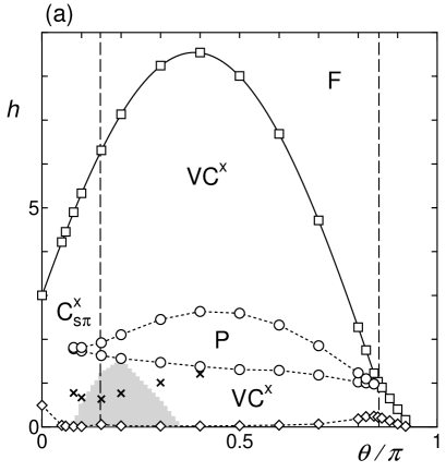
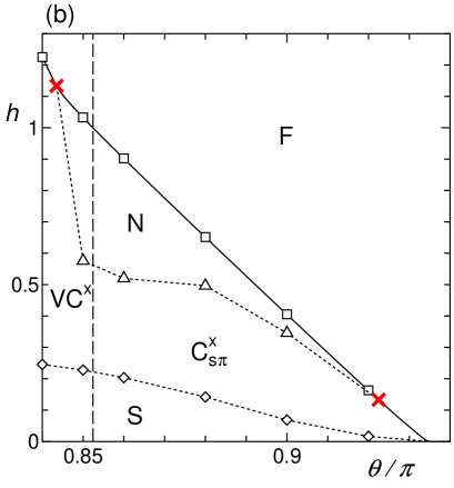
Figure 1: (a) Magnetic phase diagram of the ring-exchange model (1) for $0\leq\theta\leq\pi$, where $J_{\rm rung}=J_{\rm leg}=J=\cos\theta$ and $J_{4}=\sin\theta$. Symbols “P”, “C${}^{x}_{\rm s\pi}$”, “VC^x”, “F” denote the regions of the magnetization plateau, transverse-spin-dominant TL liquid, vector-chirality-dominant TL liquid, and fully-polarized state, respectively. Circles represent the critical fields of the plateau boundaries, $h_{\rm p1}$ and $h_{\rm p2}$, while the squares, diamonds, crosses respectively show the saturation field $h_{\rm s}$, boundaries $h_{\rm c}$ of the phases at zero magnetization, and the field $h_{\rm cusp}$ at the cusp singularity. Solid curve show the saturation field obtained from the exact-diagonalization calculation (see text in Sec. 4.3). Vertical dashed lines are the self-dual lines I and II. The shaded area around $\theta\sim 0.2\pi$ and small $h$ indicates a region where the dominant correlation is not identified. Dotted curves are a guide for eye. (b) Enlarged phase diagram for $0.84\pi<\theta<0.94\pi$. Symbols “N” and “S” denote the nematic and spin-singlet phases, respectively, while triangles and diamonds show the boundaries of the phases. The bold crosses represent the boundaries of the region of two-magnon bound pairs, $\theta_{\rm mp1}$ and $\theta_{\rm mp2}$.

4.1 Magnetization plateau

We first discuss the magnetization curve. To obtain it, we have calculated the lowest energy $E_{0}(M)$ of the Hamiltonian $\mathcal{H}_{0}$ [Eq. (2)] in a subspace characterized by the total magnetization per rung, $M=S^{z}_{\rm tot}/L_{\rm r}$, where $S^{z}_{\rm tot}=\sum_{l}(s^{z}_{1,l}+s^{z}_{2,l})$ and $L_{\rm r}$ is the number of rungs. Note that $M=1$ for the saturated state. We then determine the ground-state magnetization $M(h)$ by searching for the magnetization $M$ which minimizes the energy $E_{0}(M;h)=E_{0}(M)-hS^{z}_{\rm tot}$ for a given field $h$. The calculation was performed by the DMRG method[46, 47, 48] for the finite systems with $L_{\rm r}=31,41$, and $51$. (The reason to use the systems with odd $L_{\rm r}$ will be discussed later.) The open boundary condition was imposed for the sake of the efficiency of the DMRG method.

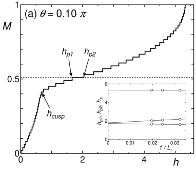
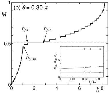
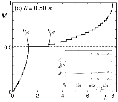
Figure 2: Magnetization curve for (a) $\theta=0.10\pi$, (b) $\theta=0.30\pi$, (c) $\theta=0.50\pi$, and (d) $\theta=0.80\pi$. The system size is $L_{\rm r}=51$ and the number of the kept states in the DMRG calculation is up to $250$. The horizontal dotted line represents the magnetization at the plateau $M=(L_{\rm r}+1)/(2L_{\rm r})$. Insets in each panel show the $1/L_{\rm r}$-dependence of the fields at the plateau boundaries, $h_{\rm p1}$ and $h_{\rm p2}$, and the saturated field $h_{\rm s}$.

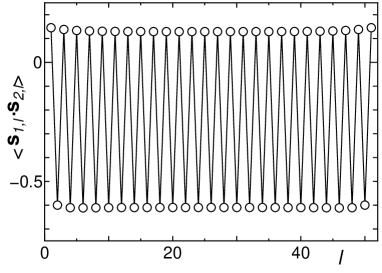
Figure 3: Local spin correlation at each rung, $\langle{\bf s}_{1,l}\cdot{\bf s}_{2,l}\rangle$, in the magnetization plateau at $\theta=0.50\pi$ and $L_{\rm r}=51$.

Figure 2 shows the magnetization curves for typical values of $\theta$ and $L_{\rm r}=51$. It is clearly seen in the figure that the magnetization curve exhibits a plateau at the magnetization $M=1/2$. [To be precise, for the open ladders with odd $L_{\rm r}$ the plateau appears at the magnetization $M=(L_{\rm r}+1)/(2L_{\rm r})$, which converges $M\to 1/2$ as $L_{\rm r}\to\infty$.] After the system-size extrapolation of the magnetic field at the upper and lower bounds of the plateau, $h_{\rm p1}$ and $h_{\rm p2}$, we find that the plateau emerges for a wide range of $\theta$, $\theta_{\rm p1}<\theta<\theta_{\rm p2}$, where the critical values are estimated to be $\theta_{\rm p1}=(0.07\pm 0.01)\pi$ and $\theta_{\rm p2}=(0.83\pm 0.01)\pi$. The estimate of the lower critical value $\theta_{\rm p1}$ is consistent with the previous result $\theta_{\rm p1}=0.069$ obtained by the exact diagonalization.[38] The extrapolated values of $h_{\rm p1}$ and $h_{\rm p2}$ as well as the saturation field $h_{\rm s}$ and the energy gap at zero magnetization $h_{\rm c}$ are plotted in the phase diagram Fig. 1.

It has been predicted by the perturbation theory around the limit of the strong rung-coupling[38] that the ground state in the plateau has the LRO of the staggered pattern of rung-singlet and triplet states. To confirm this, we have computed the ground-state expectation value of the correlation between the two spins in each rung, $\langle{\bf s}_{1,l}\cdot{\bf s}_{2,l}\rangle$. The results for $\theta=0.5\pi$ are shown in Fig. 3. The data clearly demonstrate the appearance of the LRO in the plateau state: The rungs at the open edges are almost in the spin-triplet state and the staggered pattern of triplet and singlet rungs penetrates into the bulk without a decay. Therefore, the translational symmetry is broken spontaneously in the plateau and the system has the two-fold degenerate ground states, being consistent with the necessary condition for the presence of the plateau.[49] We note that one of the two ground states is selected in the DMRG calculation due to the open boundaries. (This is the reason to select odd $L_{\rm r}$ in the analysis of magnetization plateau; for even $L_{\rm r}$, there appears a kink between two different patterns from the open boundaries at the center of the ladder, resulting in an artificial step in the plateau of the magnetization curve.) The appearance of the LRO is observed for the whole parameter regime of the magnetization plateau.

Another feature to be noted for the magnetization curve is a cusp singularity appearing at a magnetization $M<1/2$. [See Fig. 2 (a) and (b).] The cusp is found for $\theta_{\rm p1}<\theta<0.5\pi$, which corresponds to the region where the plateau exists and the bilinear exchanges are antiferromagnetic. We note that such a cusp singularity, which suggests a change of the structure of the excitation spectrum, is often observed in frustrated spin systems.[50] The strength of the field at the cusp, $h_{\rm cusp}$, is also plotted in the phase diagram, Fig. 1.

4.2 Vector chirality

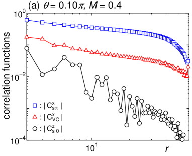
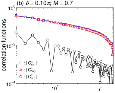
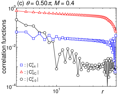
Figure 4: Absolute values of correlation functions for (a) $(\theta,M)=(0.1\pi,0.4)$, (b) $(0.1\pi,0.7)$, (c) $(0.5\pi,0.4)$, and (d) $(0.5\pi,0.7)$. Squares, triangles, and circles represent the correlation functions $C^{x}_{\rm s\pi}(r)$, $C^{x}_{\rm vc}(r)$, and $C^{z}_{\rm s0}(r)$, respectively. The system size is $L_{\rm r}=60$ and the number of the kept states in the DMRG calculation is up to $300$. Truncation errors are smaller than the size of the symbols.

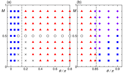
Figure 5: Dominant correlation functions for (a) $0\leq\theta\leq 0.8\pi$ and (b) $0.8\pi<\theta\leq 0.9\pi$. Squares, triangles, and diamonds represent the critical states where the transverse Néel-type-spin, transverse vector-chirality, and magnon-pairing correlation functions are dominant, respectively. Open circles show the plateau state. Vertical dashed lines are the self-dual lines I and II. Crosses denote the point where boundary effects are too strong to determine the dominant order.

Besides the gapped phases of the zero magnetization and the magnetization plateau, there is a wide region of critical states in the phase diagram. To characterize the critical states and identify the dominant order, we have calculated various two-point correlation functions in the ground state of the finite open ladders with up to $L_{\rm r}=60$ rungs using the DMRG method. The correlation functions considered are the ones of total ($q_{y}=0$) rung spin $s^{\alpha}_{1,l}+s^{\alpha}_{2,l}$ ($\alpha=x,z$), Néel-type ($q_{y}=\pi$) rung spin $s^{\alpha}_{1,l}-s^{\alpha}_{2,l}$, vector chirality $({\bf s}_{1,l}\times{\bf s}_{2,l})^{\alpha}$, scalar chirality ${\bf s}_{1,l}\cdot({\bf s}_{2,l}\times{\bf s}_{1,l+1})$, staggered dimers ${\bf s}_{1,l}\cdot{\bf s}_{1,l+1}-{\bf s}_{2,l}\cdot{\bf s}_{2,l+1}$, and two-magnon pairing operators $s^{+}_{1,l}s^{+}_{2,l}$ and $s^{+}_{1,l}s^{+}_{1,l+1}$. To lessen the open boundary effects, we calculated the correlation functions on six different pairs of two rungs $(l,l^{\prime})$ for each distance $r=|l-l^{\prime}|$, selecting the center position $l_{0}=(l+l^{\prime})/2$ to be as close as possible to the center of the ladder . We then took the average as an estimate of the correlation function for each distance $r$.

Among the correlation functions considered, the transverse Néel-type-rung-spin and vector-chirality correlation functions,

$$C^{x}_{\rm s\pi}(r) = \frac{1}{S^{2}}\langle(s^{x}_{1,l}-s^{x}_{2,l})(s^{x}_{1,l^{\prime}}-s^{x}_{2,l^{\prime}})\rangle,$$ (17)

$$C^{x}_{\rm vc}(r) = \frac{1}{S^{4}}\langle({\bf s}_{1,l}\times{\bf s}_{2,l})^{x}({\bf s}_{1,l^{\prime}}\times{\bf s}_{2,l^{\prime}})^{x}\rangle,$$ (18)

turn out to be dominant in the critical phase for $\theta\lesssim 0.84\pi$. In Fig.  4, we show the data of these correlation functions with the longitudinal total-rung-spin one,

$$C^{z}_{\rm s0}(r)=\frac{1}{S^{2}}\left[\langle(s^{z}_{1,l}+s^{z}_{2,l})(s^{z}_{1,l^{\prime}}+s^{z}_{2,l^{\prime}})\rangle-\langle s^{z}_{1,l}+s^{z}_{2,l}\rangle\langle s^{z}_{1,l^{\prime}}+s^{z}_{2,l^{\prime}}\rangle\right].$$ (19)

The Néel-type rung-spin correlation $C^{x}_{\rm s\pi}(r)$ and vector-chirality one $C^{x}_{\rm vc}(r)$ decay algebraically, oscillating with the wavenumber $q_{x}=\pi$. Since the decay exponents of these correlations seem to be the same, we determine which is the dominant one by comparing their amplitudes. Figure 5 summarizes the results in the $\theta$ versus $M$ plane. The Néel-type rung-spin correlation $C^{x}_{\rm s\pi}(r)$ is dominant for $\theta<\theta_{\rm sdI}$ while the vector-chirality one $C^{x}_{\rm vc}(r)$ is for $\theta>\theta_{\rm sdI}$: The crossover occurs at the self-dual line I, as discussed in Sec. 3. The difference between the amplitudes of $C^{x}_{\rm s\pi}(r)$ and $C^{x}_{\rm vc}(r)$ becomes smaller as the magnetization $M$ increases and they converge the same value at $M\to 1$ (see Fig. 4). The vector-chirality-dominant TL liquid thus emerges in the wide parameter space of strong ring exchange including both the regions of the antiferromagnetic and ferromagnetic bilinear exchanges. We note that there remains a small region around $\theta\sim 0.2\pi$ and small $M$ where too strong open boundary effects prevent us from determining the dominant correlation functions. For clarifying the nature of the model in the region, it is required to perform the calculation for much larger systems, which is out of the scope of our numerics and left for future studies.

We mention the possible “$\eta$-inversion” in the system. For the present model (1), it was predicted that around the plateau there is a parameter regime where the longitudinal incommensurate spin correlation function becomes stronger than the transverse staggered spin one.[39] We have found that for $M>0.5$ the decay exponent of the longitudinal total-rung-spin correlation function $C^{z}_{\rm s0}(r)$ approaches those of $C^{x}_{\rm s\pi}(r)$ and $C^{x}_{\rm vc}(r)$ as $M$ decreases and they seem very close to each other at $M=0.6$. This seems consistent with the prediction. However, unfortunately, we do not obtain a clear evidence of the phenomenon because of the incommensurate character of $C^{z}_{\rm s0}(r)$ as well as the open boundary effects, which make it difficult to estimate the decay exponent of $C^{z}_{\rm s0}$ precisely. To overcome the difficulties, numerical calculations for larger systems and, more preferably, theoretical descriptions such as the bosonization analysis for the low-energy states of the system would be necessary.

4.3 Nematic phase

Figure 6: (a) Magnetization curve for $\theta=0.88\pi$. The system size is $L_{\rm r}=51$. (b) Field dependence of excitation energy $E_{0}(M;h)-E_{\rm gs}(h)$. Solid and dotted lines represent the energy level with even and odd $S^{z}_{\rm tot}$, respectively.

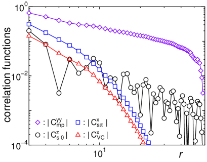
Figure 7: Absolute values of correlation functions for $(\theta,M)=(0.88\pi,0.7)$. Diamonds, circles, squares, and triangles represent the correlation functions $C^{yy}_{\rm mp}(r)$, $C^{z}_{\rm s0}(r)$, $C^{x}_{\rm s\pi}(r)$, and $C^{x}_{\rm vc}(r)$, respectively. The system size is $L_{\rm r}=60$ and the number of the kept states in the DMRG calculation is up to $300$. Truncation errors are smaller than the size of the symbols.

Here, we discuss our results for $\theta\gtrsim 0.84\pi$, where we find the nematic phase. Figure 6 (a) shows the magnetization curve obtained by the DMRG calculation for $\theta=0.88\pi$. An interesting feature is that for a field $h$ larger than a certain critical value the magnetization changes by a step $\Delta S^{z}_{\rm tot}=2$. This suggests that magnons in the background of the saturated state form bound pairs of two magnons. To confirm this, we calculate the field dependence of the excitation spectrum of the lowest level in each subspace of $M$, $E_{0}(M;h)-E_{\rm gs}(h)$, where $E_{\rm gs}(h)$ is the ground-state energy under a field $h$. The result in Fig. 6 (b) clearly indicates that for large $h$ only the levels with odd $S^{z}_{\rm tot}$ becomes the ground state while the levels with even $S^{z}_{\rm tot}$ always have a finite excitation energy. We thereby conclude that the magnons indeed form two-magnon bound pairs with a finite binding energy. [Note that, since $L_{\rm r}$ is odd, even (odd) magnons are included in the state with odd (even) $S^{z}_{\rm tot}$.]

Since the magnetization curve in Fig. 6 was calculated for the system with the open boundary condition, one may think that the step by $\Delta S^{z}_{\rm tot}=2$ is due to open boundary effects. To answer the question and determine the boundary of the region of the magnon pairs more accurately, we have performed the exact diagonalization calculation for the periodic ladder within the subspace of $n$-magnon states, where the number of magnons is up to $n=4$. The system size treated was up to $L_{\rm r}=48$, which turned out to be large enough. We calculate the lowest energy in each subspace and analyze the magnon instability in the saturated state. We thereby find that for $\theta<\theta_{\rm mp1}=0.844\pi$ the single-magnon instability is the strongest and the saturation field is given by $h_{\rm s}=3J+8J_{4}=3\cos\theta+8\sin\theta$, which is obtained analytically. However, when $\theta$ exceeds $\theta_{\rm mp1}$, the two-magnon instability dominates and determines the saturation field $h_{\rm s}$. The region of two-magnon bound pairs extends for $\theta_{\rm mp1}<\theta<\theta_{\rm mp2}=0.923\pi$. In the small region between $\theta_{\rm mp2}$ and the boundary of the ferromagnetic phase $\theta=0.935\pi$, we find that four-magnon instability takes place, but we must note that the instability of more-magnon bound pairs may emerge in the vicinity of the ferromagnetic phase. The saturation field obtained and the boundaries of the two-magnon pairing region, $\theta_{\rm mp1}$ and $\theta_{\rm mp2}$, are plotted in Fig. 1.

To investigate the nature of the system in the magnon-pairing regime in more detail, we have calculated the several correlation functions mentioned above using the DMRG method. From the calculation, it turns out that the magnon-pairing correlation functions,

$$C^{yy}_{\rm mp}(r) = \frac{1}{S^{4}}\langle s^{+}_{1,l}s^{+}_{2,l}s^{-}_{1,l^{\prime}}s^{-}_{2,l^{\prime}}\rangle,$$ (20)

$$C^{xx}_{\rm mp}(r) = \frac{1}{S^{4}}\langle s^{+}_{1,l}s^{+}_{1,l+1}s^{-}_{1,l^{\prime}}s^{-}_{1,l^{\prime}+1}\rangle,$$ (21)

$$C^{xy}_{\rm mp}(r) = \frac{1}{S^{4}}\langle s^{+}_{1,l}s^{+}_{1,l+1}s^{-}_{1,l^{\prime}}s^{-}_{2,l^{\prime}}\rangle,$$ (22)

dominate in the region where the two-magnon bound pairs are found. A typical example of the data of $C^{yy}_{\rm mp}(r)$ are shown in Fig. 7 with the longitudinal total-rung-spin correlation $C^{z}_{\rm s0}(r)$, the transverse Néel-type rung-spin one $C^{x}_{\rm s\pi}(r)$, and the transverse vector-chirality one $C^{x}_{\rm vc}(r)$. The magnon-pairing correlation function $C^{yy}_{\rm mp}(r)$ is clearly the strongest: $C^{z}_{\rm s0}(r)$ decays algebraically but faster than $C^{yy}_{\rm mp}(r)$ while $C^{x}_{\rm s\pi}(r)$ and $C^{x}_{\rm vc}(r)$ decay exponentially. We note that the other magnon-pairing correlation functions $C^{xx}_{\rm mp}(r)$ and $C^{xy}_{\rm mp}(r)$ also decay algebraically with the same exponent as that of $C^{yy}_{\rm mp}(r)$ while the amplitudes are different. Interestingly, the magnon-pairing correlation functions have the sign $C^{yy}_{\rm mp}(r)>0$, $C^{xx}_{\rm mp}(r)>0$, and $C^{xy}_{\rm mp}(r)<0$ for arbitrary distance $r$; they exhibit the “$d$-wave-like” symmetry. All these behaviors are in common with those of the nematic phase found for the ring-exchange model in the square lattice,[31] in which phase the two-magnon bound pairs undergo a bose condensation resulting in the magnon-pairing order, though in our one-dimensional system the true LRO of the pairing correlation is destroyed by a strong quantum fluctuation. We therefore conclude the ring-exchange ladder (1) for the parameter regime is in (one-dimensional analog of) the nematic phase. The region of the nematic phase, where we find the magnon-bound pairs and the dominant magnon-pairing quasi-LRO, are shown in Figs. 1 (b) and 5 (b). The phase appears at the fields $h$ larger than a critical value $h_{\rm mp}$ and extends over the self-dual line II. This is allowed since the magnon-pairing order parameter is self-dual under the duality transformation. The decay exponents of the magnon-pairing correlation $C^{yy}_{\rm mp}(r)$ and longitudinal total-rung-spin one $C^{z}_{\rm s0}(r)$ become closer to each other as the magnetization decreases and seem almost the same for $\theta=0.85$ and $M=0.3$.

At a field $h$ lower than the critical value $h_{\rm mp}$, we find that the vector-chirality correlation $C^{x}_{\rm vc}(r)$ is dominant for $\theta<\theta_{\rm sdII}$ while the Néel-type-rung-spin one $C^{x}_{\rm s\pi}(r)$ with wavenumber $q_{x}=0$ along the leg direction dominates for $\theta>\theta_{\rm sdII}$. The crossover between the vector-chirality-dominant and Néel-type-spin-dominant TL liquids occurs at the self-dual line II, as expected in Sec. 3.

5 Summary and Concluding remarks

In summary, we have studied the spin-$1/2$ two-leg Heisenberg ladder with four-spin ring exchanges under a magnetic field, for a wide parameter regime including both the antiferromagnetic and ferromagnetic bilinear couplings. We have introduced a duality transformation, which is a simple extension of the spin-chirality duality transformation developed previously[26, 27] but leads to a nontrivial duality mappings on coupling parameters in the Hamiltonian as well as order parameters. These dualities yield two self-dual lines in the parameter space of the ring-exchange ladder (1).

Further, using the density-matrix renormalization-group and exact diagonalization methods, we have determined numerically the magnetic phase diagram, Fig. 1, including the magnetization plateau at $M=1/2$ and the regions of TL liquids with different dominant quasi-LRO. We have found the vector-chirality-dominant TL liquid emerging in a wide parameter regime of the strong ring-exchange coupling between the self-dual lines, while there appear TL liquids with the dominant transverse spin quasi-LRO outside of the self-dual lines. Moreover, we have identified the nematic phase, in which the magnons form bound pairs and the condensation of the bound pairs leads to the dominant magnon-pairing correlation functions, in a finite regime in the vicinity of the ferromagnetic phase.

The formation of the magnon bound pairs and their condensation in the nematic phase are not peculiar to the ring-exchange ladder (1) but are found in various $S=1/2$ systems: The phenomena have been reported for the ring-exchange model in the square lattice[31] and triangular lattice,[36] and the zigzag ladder with ferromagnetic nearest-neighbor and antiferromagnetic next-nearest-neighbor couplings.[51, 52, 53, 54] These observations suggest that the phenomena are a general feature of “frustrated ferromagnets” in which the fully-polarized state is destabilized by certain perturbations such as ring exchange and/or antiferromagnetic couplings. Systematic studies to develop theoretical descriptions of the state and to clarify the relation between the nematic phases in $S=1/2$ and $S\geq 1$ systems would be important for understanding the phenomena.

For the two-leg ladder with extended four-spin exchange $\mathcal{H}_{\rm ext}$ [Eq. (6)], it was predicted in Ref. Sato2007 that the model under a magnetic field $h>0$ could realize the true LRO of the longitudinal vector-chirality $({\bf s}_{1,l}\times{\bf s}_{2,l})^{z}$, while the author also pointed out that the form of the ring-exchange coupling, $J_{\rm rr}=J_{\rm ll}=-J_{\rm dd}$, was not suitable for the appearance of the LRO. Indeed, we have not observed the appearance of the true LRO of the vector-chirality in our calculation on the ring-exchange ladder (1). Searching for the LRO in a ladder model with the generalized four-spin exchanges of more suitable form would be an interesting issue.

References

- [1] M. Roger, J.H. Hetherington, and J.M. Delrieu: Rev. Mod. Phys. 55 (1983) 1, and references therein.
- [2] M. Roger: Phys. Rev. B 30 (1984) 6432.
- [3] D.S. Greywall and P.A. Busch: Phys. Rev. Lett. 62 (1989) 1868.
- [4] M. Roger: Phys. Rev. Lett. 64 (1990) 297.
- [5] M. Roger, C. Bäuerle, Y.M. Bunkov, A.-S. Chen, and H. Godfrin: Phys. Rev. Lett. 80 (1998) 1308.
- [6] T. Okamoto and S. Kawaji: Phys. Rev. B 57 (1998) 9097.
- [7] M. Katano and D.S. Hirashima: Phys. Rev. B 62 (2000) 2573.
- [8] B. Bernu, L. Cândido, and D.M. Ceperley: Phys. Rev. Lett. 86 (2001) 870.
- [9] S. Brehmer, H.-J. Mikeska, M. Müller, N. Nagaosa, and S. Uchida: Phys. Rev. B 60 (1999) 329.
- [10] M. Matsuda, K. Katsumata, R.S. Eccleston, S. Brehmer, and H.-J. Mikeska: Phys. Rev. B 62 (2000) 8903.
- [11] M. Matsuda, K. Katsumata, R.S. Eccleston, S. Brehmer, and H.-J. Mikeska: J. Appl. Phys. 87 (2000) 6271.
- [12] K.P. Schmidt, C. Knetter, and G.S. Uhrig: Europhys. Lett. 56 (2001) 877.
- [13] T.S. Nunner, P. Brune, T. Kopp, M. Windt, and M. Grüninger: Phys. Rev. B 66 (2002) 180404(R).
- [14] Y. Honda, Y. Kuramoto, and T. Watanabe: Phys. Rev. B 47 (1993) 11329.
- [15] Y. Mizuno, T. Tohyama, and S. Maekawa: J. Low Temp. Phys. 117 (1999) 389.
- [16] Y. Mizuno, T. Tohyama, and S. Maekawa: J. Phys. Chem. Sol. 62 (2001) 273.
- [17] R. Coldea, S.M. Hayden, G. Aeppli, T.G. Perring, C.D. Frost, T.E. Mason, S.-W. Cheong, and Z. Fisk: Phys. Rev. Lett. 86 (2001) 5377.
- [18] A.A. Katanin and A.P. Kampf: Phys. Rev. B 66 (2002) 100403(R).
- [19] A.A. Katanin and A.P. Kampf: Phys. Rev. B 67 (2003) 100404(R).
- [20] A.D. Klironomos, J.S. Meyer, and K.A. Matveev: Europhys. Lett. 74 (2006) 679.
- [21] A.D. Klironomos, J.S. Meyer, T. Hikihara, and K.A. Matveev: Phys. Rev. B 76 (2007) 075302.
- [22] Y. Honda and T. Horiguchi: arXiv:cond-mat/0106426 (unpublished).
- [23] K. Hijii and K. Nomura: Phys. Rev. B 65 (2002) 104413.
- [24] M. Müller, T. Vekua, and H.-J. Mikeska: Phys. Rev. B 66 (2002) 134423.
- [25] A. Läuchli, G. Schmid, and M. Troyer: Phys. Rev. B 67 (2003) 100409(R).
- [26] T. Hikihara, T. Momoi, and X. Hu: Phys. Rev. Lett. 90 (2003) 087204.
- [27] T. Momoi, T. Hikihara, M. Nakamura, and X. Hu: Phys. Rev. B 67 (2003) 174410.
- [28] V. Gritsev, B. Normand, and D. Baeriswyl: Phys. Rev. B 69 (2004) 094431.
- [29] A. Chubukov, E. Gagliano, and C. Balseiro: Phys. Rev. B 45 (1992) 7889.
- [30] A. Läuchli, J.C. Domenge, C. Lhuillier, P. Sindzingre, and M. Troyer: Phys. Rev. Lett. 95 (2005) 137206.
- [31] N. Shannon, T. Momoi, and P. Sindzingre: Phys. Rev. Lett. 96 (2006) 027213.
- [32] T. Momoi, K. Kubo, and K. Niki: Phys. Rev. Lett. 79 (1997) 2081.
- [33] K. Kubo and T. Momoi: Z. Phys. B 103 (1997) 485.
- [34] G. Misguich, B. Bernu, C. Lhuillier, and C. Waldtmann: Phys. Rev. Lett. 81 (1998) 1098.
- [35] G. Misguich, C. Lhuillier, B. Bernu, and C. Waldtmann: Phys. Rev. B 60 (1999) 1064.
- [36] T. Momoi, P. Sindzingre, and N. Shannon: Phys. Rev. Lett. 97 (2006) 257204.
- [37] T. Sakai and Y. Hasegawa: Phys. Rev. B 60 (1999) 48.
- [38] A. Nakasu, K. Totsuka, Y. Hasegawa, K. Okamoto, and T. Sakai: J. Phys.: Condens. Matter 13 (2001) 7421.
- [39] T. Sakai and K. Okamoto: J. Phys. Chem. Sol. 66 (2005) 1450.
- [40] M. Sato: Phys. Rev. B 76, (2007) 054427.
- [41] R. Chitra and T. Giamarchi: Phys. Rev. B 55 (1997) 5816.
- [42] M. Usami and S. Suga: Phys. Rev. B 58 (1998) 14401.
- [43] T. Giamarchi and A.M. Tsvelik: Phys. Rev. B 59 (1999) 11398.
- [44] A. Furusaki and S.C. Zhang: Phys. Rev. B 60 (1999) 1175.
- [45] T. Hikihara and A. Furusaki: Phys. Rev. B 63 (2001) 134438.
- [46] S. R. White: Phys. Rev. Lett. 69 (1992) 2863.
- [47] S. R. White: Phys. Rev. B 48 (1993) 10345.
- [48] S. R. White: Phys. Rev. Lett. 77 (1996) 3633.
- [49] M. Oshikawa, M. Yamanaka, and I. Affleck: Phys. Rev. Lett. 78 (1997) 1984.
- [50] See, for example, K. Okunishi, Y. Hieida, and Y. Akutsu: Phys. Rev. B 60 (1999) R6953.
- [51] A. V. Chubukov: Phys. Rev. B 44 (1991) 4693.
- [52] F. Heidrich-Meisner, A. Honecker, and T. Vekua: Phys. Rev. B 74 (2006) 020403(R).
- [53] T. Vekua, A. Honecker, H.-J. Mikeska, and F. Heidrich-Meisner: arXiv:0704.0764 (unpublished).
- [54] L. Kecke, T. Momoi, and A. Furusaki: arXiv:0708.0701 (unpublished).