A probabilistic regulatory network for the human immune system.

Abstract.

In this paper we made a review of some papers about probabilistic regulatory networks (PRN), in particular we introduce our concept of homomorphisms of PRN with an example of projection of a regulatory network to a smaller one. We apply the model PRN ( or Probabilistic Boolean Network) to the immune system, the PRN works with two functions. The model called ”The B/T-cells interaction” is Boolean, so we are really working with a Probabilistic Boolean Network. Using Markov Chains we determine the state of equilibrium of the immune response.

1. Introduction

The biological process can be modeled using different class of models, but in most of the applications differential equation models have been selected because the entities can have more than two values. Here we use a probabilistic regulatory network model, that it is a discrete model with only a finite number of state and activities. In particular, we describe the dynamic of the immune response in humans, using the Boolean model called B/T-cells [8], and we added probabilities and use the dynamic model of Probabilistic Boolean Network, [10, 11, 12, 13, 14].

The immune system is separated by functionality in two parts: recognition and effector functions. A complex immune system has cells and molecules that give us a basic defense against bacteria, viruses, fungi, and other pathogenic agents. Possibly, it has tens or hundreds of different types of regulatory and effector molecules. So, an important role in the study of this class of system plays the reduction of networks, for that reason we introduce the concept of projection of one net to another smaller for the future applications. A variety of cell types compose the immune system, the most important are the lymphocytes. These cells are created in the bone marrow, along with all of the other blood cells, and are transported throughout the body via the blood stream. Lymphocytes spend considerable time resident in lymphoid organs, such as the bone marrow, the thymus, the spleen, and lymph nodes. Lymphocytes are subdivided in two classes: B-cells and T-cells, see Perelson [9]. B lymphocytes secrete antibodies, and the main function of T-cells is the interacting with other cells. Helper T cells act through the secretion of lymphokines, they made possible to transform the B-cells into an antibody-secreting state. Helper T-cells are the cells that are predominantly infected by the human immunodeficiency virus, and plays a major role in AIDS. Cytotoxic T-cells, are responsible for killing virally infected cells and cells that look like abnormal, such as some tumor cells.

In this paper we study the dynamic of the B/T-cell model giving by Kaufman, Urbain, and Thomas, n 1985. In this model they use functions, in which a boolean parameter appears, and they obtained the steady state of the system, in our case we describe in a more complex way the immune system using probabilities for the two possible functions of activity. Our model can be changed for another more complex if we consider a three values model instead of a Boolean model

2. Preliminaries and projection

In this section we introduce the mathematical background of the model Probabilistic Regulatory Network, and the concept of projection using and example. For the complete mathematical background we suggest to see, [3, 5, BL]. Here, we give a method that permit us to build regulatory networks with probabilities assigned to its functions. We use an algorithm for understanding the concept of Probabilistic Regulatory Network.

2.1. Algorithm

Input:

1. $n=$ number of entities in the network under studying, for example 100 genes, and the set of values for each entity, that we denote by $k_{a}$.
2. A set of relations $\{m_{a,b}\}$ taking $1$ if the entity $a$ is related to the entity $b$, and $0$ otherwise.
3. A set of finite families of states in the network which gives the time series data for one, two or more update functions, $A_{1}=\{(a^{1}_{i,1},\ldots,a^{2}_{i,n-1},a^{1}_{i,n})|1\leq i\leq m_{x}\},$ $\ldots$, and $A_{s}=\{(a^{s}_{i,1},\ldots,a^{s}_{i,n-1},a^{s}_{i,n})|1\leq i\leq m_{s}\}$.
4. A set of values $C=\{c_{1},\ldots,c_{s}\}$ with $s$ probabilities obtained in some way by the experiment or by the time series data. That is $c_{1}+\cdots+c_{s}=1,$ and $c_{i}\in[0,1]$.

• Creation the low level graph $\Gamma$:

  • $n=3$ , and $m_{12}=1$ , $m_{23}=1$ , y $m_{13}=0$, then our net is very simple and it is the following:

    $$\hskip 21.68121pt\Gamma\ \hskip 21.68121pt\ \begin{array}[]{ccc}&&\bullet\ 3\\ &&\mid\\ 1\ \bullet&{\overline{\hskip 14.45377pt}}&\bullet\ 2\end{array},\hskip 21.68121pt\$$

• We define the set where the functions are acting, in our case, they are boolean, that is $k_{1}=\{0,1\}=k_{2}=k_{3}=\mathbb{Z}_{2}$, considering $k=k_{1}\times k_{2}\times k_{3}=\{0,1\}^{3}$. The two sequential states are the following:

  Time series data 1 $A_{1}=\{(0,1,0),(1,1,1),(1,1,0),(1,1,1)\}$.

  Time series data 2 $A_{2}=\{(0,1,0),(0,1,1),(0,1,0),(0,1,1)\}$.
  

  We obtain two different update functions:

  $$f_{1}(x_{1},x_{2},x_{3})=(1,x_{2},x_{2}(x_{3}+1)),\ and\ f_{2}(x_{1},x_{2},x_{3})=(x_{1},x_{2},x_{2}(x_{3}+1)).$$

• We assign the following probabilities to each update function: $2/3$ to the function $f_{1}$, and $1/3$ for the function $f_{2}$.

• We construct the high level digraph, that is the following in this example

Output:

$$States\ Space$$

$$\begin{array}[]{ccc}\overset{1}{\circlearrowright}\underbrace{\overbrace{(1,0,0)}}&\overset{1}{\leftarrow}&\underbrace{\overbrace{(1,0,1)}}\\ {}^{2/3}\uparrow&{}^{2/3}\nwarrow&\\ \underbrace{\overbrace{(0,0,1)}}&\overset{1/3}{\rightarrow}&\underbrace{\overbrace{(0,0,0)}}\overset{1/3}{\circlearrowleft}\\ \end{array}\ \hskip 21.68121pt\begin{array}[]{ccc}\underbrace{\overbrace{(0,1,0)}}&\overset{1/3}{\leftrightarrows}&\underbrace{\overbrace{(0,1,1)}}\\ {}^{2/3}\downarrow&&{}^{2/3}\downarrow\\ \underbrace{\overbrace{(1,1,1)}}&\overset{1}{\leftrightarrows}&\underbrace{\overbrace{(1,1,0)}}\\ \end{array}$$

In order to study the dynamic we need the Transition Matrix of the system, because we have two functions acting on the set of states. So the dynamic will be study using Markov Chains. First we use the following order for the states, but this is not the only possibility

$$\begin{array}[]{cccccccc}(0,0,0)&(0,0,1)&(1,0,0)&(1,0,1)&(0,1,1)&(1,1,0)&(0,1,0)&(1,1,1)\\ 1&2&3&4&5&6&7&8\\ \end{array}$$

The matrix is constructed in the following way $a_{(i,j)}$ is the probability to have the arrow that it is going from $i$ to $j$, then $a_{(2,3)}=p(f_{2})=1/3$, but $a_{(3,3)}=p(f_{2})+p(f_{1})=1$ because the two functions are going from $(1,0,0)$ to $(1,0,0)$.

$$T=\left[\begin{array}[]{cccc|cccc}0&2/3&1/3&0&0&0&0&0\\ 2/3&0&1/3&0&0&0&0&0\\ 0&0&1&0&0&0&0&0\\ 0&0&1&0&0&0&0&0\\ \hline\cr 0&0&0&0&0&1/3&2/3&0\\ 0&0&0&0&0&0&0&1\\ 0&0&0&0&2/3&0&0&1/3\\ 0&0&0&0&0&1&0&0\\ \end{array}\right]$$

The dynamic of the systems is going to stationary states, or the knowing by the equilibrium of the system. we have this information with the iteration of the matrix, that is computing the power of the transition matrix until we have the same vector in each arrow of the matrix. In this very simple case we have two separated spaces, so our matrix works with two sub matrices of $T$: $T_{11}$ and $T_{22}$, in fact

$$T_{11}\rightarrow\left[\begin{array}[]{cccc}0&0&1&0\\ 0&0&1&0\\ 0&0&1&0\\ 0&0&1&0\\ \end{array}\right]$$

meanwhile for the other submatrix $T_{22}$ we have:

$$T_{22}\rightarrow\left[\begin{array}[]{cccc}0&0&0&1\\ 0&1&0&0\\ 0&1&0&0\\ 0&0&0&1\\ \end{array}\right]$$

This induce that the equilibrium of the systems is the following

$$\pi=(0,0,.5,0,0,.25,0,.25)$$

That is, the system is going to the boolean vector $(1,0,0)$ with a probability of .5, to the boolean vectors $(1,1,0),\ (1,1,1)$, with probability of $.25$. We consider that, additionally some part of this systems is going from $(1,1,0)$ to $(1,1,1),$ and from $(1,1,1)$ to $(1,1,0)$ continuously.

3. Projection and Reduction of networks

Reduction of a network is our interest in this section, we use a bigger net than the one in the last section. In particular the mathematical concept that permit us to do that is the called homomorphism. In particular here we present a projection, that it is an homomorphism which reduce the network to smaller and have the very important property to have the similar state of equilibrium, for mathematical background see [1, 2]. For other approach of the concept of homomorphism, that had applications to dynamical networks, see [4, 6, MD].

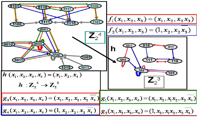
Figure 1. Projection

We have the last example and now, the following network is defined as follows: $\Delta$,

$$\hskip 28.90755pt\Delta\ \ \hskip 21.68121pt\ \ \ \begin{array}[]{ccc}2\ \bullet&{\overline{\hskip 14.45377pt}}&\bullet\ 4\\ &\diagdown&\mid\\ 1\ \bullet&{\overline{\hskip 14.45377pt}}&\bullet\ 3\end{array}\hskip 14.45377pt\$$

Each vertex has two values, that is our network is boolean $\mathbb{Z}_{2}=\{0,1\}$, then the functions act on the set ${\mathbb{Z}_{2}}^{4}$, that has $16$ elements or states. The functions are the following:

$$\begin{array}[]{ll}g_{1}(x_{1},x_{2},x_{3},x_{4})=(x_{1},x_{2},x_{1}x_{2},x_{2}\overline{x_{4}}),&g_{2}(x_{1},x_{2},x_{3},x_{4})=(1,x_{2},x_{1}x_{2},x_{2}\overline{x_{4}})\\ g_{3}(x_{1},x_{2},x_{3},x_{4})=(x_{1},x_{2},x_{2},x_{2}\overline{x_{4}}),&g_{4}(x_{1},x_{2},x_{3},x_{4})=(1,x_{2},x_{2},x_{2}\overline{x_{4}})\\ \end{array}.$$

The homomorphism is the following:

$$h(x_{1},x_{2},x_{3},x_{4})=(x_{1},x_{2},x_{4})$$

This function satisfies the following properties, that are called commutative diagrams:

$$\begin{CD}{\mathbb{Z}_{2}}^{4}@ >g_{1}>>{\mathbb{Z}_{2}}^{4}\\ @V{h}V{}V@V{h}V{}V\\ {\mathbb{Z}_{2}}^{3}@ >f_{1}>>{\mathbb{Z}_{2}}^{3}\end{CD},\ \begin{CD}{\mathbb{Z}_{2}}^{4}@ >g_{3}>>{\mathbb{Z}_{2}}^{4}\\ @V{h}V{}V@V{h}V{}V\\ {\mathbb{Z}_{2}}^{3}@ >f_{1}>>{\mathbb{Z}_{2}}^{3}\end{CD},$$

$$\begin{CD}{\mathbb{Z}_{2}}^{4}@>{g_{2}}>{}>{\mathbb{Z}_{2}}^{4}\\ @V{h}V{}V@V{h}V{}V\\ {\mathbb{Z}_{2}}^{3}@>{f_{2}}>{}>{\mathbb{Z}_{2}}^{3}\end{CD}\textrm{ y }\ \ \ \begin{CD}{\mathbb{Z}_{2}}^{4}@>{g_{4}}>{}>{\mathbb{Z}_{2}}^{4}\\ @V{h}V{}V@V{h}V{}V\\ {\mathbb{Z}_{2}}^{3}@>{f_{2}}>{}>{\mathbb{Z}_{2}}^{3}\end{CD}.$$

So, $h$ is a structural homomorphism, or an homomorphism of PBN. The probabilities are $p(g_{1})=p(g_{3})=2/3$, and $p(g_{2})=p(g_{4})=1/6$, of course the sum is 1 but this is our suggestion, because we can have others probabilities. In fact, using the Theorem in Section 4 [2], this network is going to similar states, that is the boolean vectors $(0,0,0,0),\ (0,0,1,0),\ (1,0,0,0),\ (1,0,1,0),\ (0,0,0,1),$ $\ (0,0,1,1),\ (1,0,0,1),\ (1,0,1,1)$ are going to the state $(1,0,0,0)$, and the boolean vectors $(0,1,1,0),\ (1,1,0,0),\ (0,1,0,0),\ (1,1,1,0),$ $\ (0,1,1,1),\ (1,1,0,1),\ (0,1,0,1),$ $(1,1,1,1)$ are going to the states $(1,1,1,0)$, and $(1,1,1,1)$, and the equilibrium is obtained after several iterations of the functions, that is the powers of the transition matrix give the following information.

$$\pi=(0,0,.5,0,0,0,0,0,0,0,.25,0,0,0,0,.25)$$

4. The immune system: modeling the B/T-cells interactions

The following model appears in [9], under the information that it is the model $B/T-cells$, of Kaufman, Urbain, and Thomas, described in 1985. Here we introduce an important applications of the model PBN to the understanding the immune system.

$$Model\ B/T-cells\begin{array}[]{ccccc}\underbrace{\overbrace{Antibody=a}}&\leftrightarrows&\underbrace{\overbrace{e}}&\rightarrow&\underbrace{\overbrace{T_{h}-cells}}\circlearrowleft\\ &\nwarrow&\downarrow&\swarrow&\uparrow\downarrow\\ &&\underbrace{\overbrace{B-cells}}&&\underbrace{\overbrace{T_{s}-cells}}\circlearrowleft\\ \end{array}$$

The original model had a complex presentation, using a parameter $e$, for the antigen, that has only two values, that is antigen is assumed to be either present or absent and hence is represented by $e$, a binary parameter. The binary variables are $b$, the B-cell population, $a$, the secreted antibody concentration, and $h$ and $s$, helper and suppressor T-cell populations, respectively. We use for boolean functions, the polynomial representations over the field $\mathbb{Z}_{2}$, then we have the following functions:

$$f_{b}(b,h,s,a)=eh;\ f_{h}(b,h,s,a)=e\overline{s}+h+e\overline{s}h;$$

$$f_{s}(b,h,s,a)=h+s+hs;\ f_{a}(b,h,s,a)=ebh.$$

that had obtained by the digraph in the above diagram, called ” Model B/T-cells”. Because the parameter $e$ takes two values 0, and 1, we obtain two functions:

$$f_{0}(b,h,s,a)=(0,h,h+s+hs,0);$$

$$f_{1}(b,h,s,a)=(h,\overline{s}+h+\overline{s}h,h+s+hs,bh)$$

Then, our space has $2^{4}=16$, and we can see how the system is moving to the equilibrium of the system

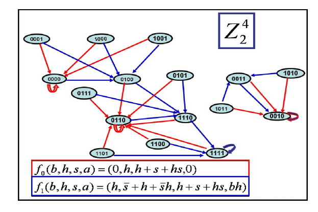
Figure 2. Espacio de estados del Modelo Booleano B/T-cell

It is easy to see that there are three steady states for the function $f_{0}$, that is when the antigen is absent, and two steady states for the function $f_{1}$, that is when the antigen is present. In [9], it is considered the function $f_{0}$ working and the same time of the function $f_{1}$ but they do not use probabilities, so the biological conclusion is not supported by a good description of the activity in the net. They consider that the stationary points of $f_{0}$ are the virgin states, that is they do not have memory about the antigen, because in those states there are only helpers and suppressors cells. But with our analysis we obtain a new results

Using Markov Chains, and assigning the same probability to each function, that is .5, the equilibrium of the system is the following

$$\pi=(.375,0,0,0,0,0,0,0,0,0,.375,0,.125,.125,0,0),$$

where the order in the set of states is the following $\{(0,0,1,0),(1,0,1,1),(0,0,1,1),$
$(1,0,1,0),(0,0,0,0),(0,0,0,1),(0,1,0,0),(1,0,0,0),(1,0,0,1),(0,1,1,1),(0,1,1,0),$
$(0,1,0,1),(1,1,1,0),(1,1,1,1),(1,1,0,0),(1,1,0,1)\}$ We suggest the following interpretation of this equilibrium. The states $(0,0,1,0),$ and $(0,1,1,0)$ are the steady states when we do not have antigen, and they have more probability to arrive for the network. Meanwhile the others two states are $(1,1,1,0)$, and $(1,1,1,1)$, when the interaction has a complete action in the network, and they had less probabilities, because the life in general, is going to the others states, maybe this happen when the helper and the suppressors cells are acting but they are not enough strong to destroy the antigen. So a better and more complex dynamical system, can work, if we consider three possibilities for the antigen, and for all variables in this particular model of interaction.

References

- [1] Maria A. Avino, Homomorphism of Probabilistic Gene Regulatory Networks, Proceedings of Workshop on Genomic Signal Processing and Statistics (GENSIPS) 2006, TX, 4 pages.
- [2] Maria A. Avino, Introducing a probabilistic structure on Sequential Dynamical Systems, Simulation and Reduction of Probabilistic Sequential Networks, preprint, 2007, 21 pages.
- [3] Maria A. Avino-Diaz, Edward Green, and Oscar Moreno, Applications of finite fields to dynamical systems and reverse engineering problem Proceedings of ACM Symposium on Applied Computing,(2004).
- [4] E. R. Dougherty and I. Shmulevich, Mappings between probabilistic Boolean networks, Signal Processing, vol. 83, no. 4, pp. 799 809, 2003.
- [5] E. Green, On polynomial solutions to reverse engineering problems. preprint, (2003)
- [6] I. Ivanov, and Edward R. Dougherty, Reduction Mappings between Probabilistic Boolean Networks, EURASIP Journal on Applied Signal Processing 2004:1, 125 131
- [7] Kauffman, S.A. The Origins of Order: Self-organization and Selection in Evolution. Oxford University Press, NY,(1993)
- [8] M. Kaufman, J. Urbain, and R. Thomas, Towards a Logical Analysis of the Immune Response 1985, J. Theor. Biol. 114, 527 561.
- [9] Alan S. Perelson, Ge rard Weisbuch, Immunology for physicists Reviews of Modern Physics, Vol. 69, No. 4, October 1997 The American Physical Society 1219-1267.
- [10] I. Shmulevich, E. R. Dougherty, S. Kim, and W. Zhang,Probabilistic Boolean networks: a rule-based uncertainly model for gene regulatory networks, Bioinformatics 18(2):261-274, (2002).
- [11] I. Shmulevich, E. R. Dougherty, and W. Zhang,Gene perturbation and intervention in probabilistic Boolean networks, Bioinformatics 18(10):1319-1331, (2002).
- [12] I. Shmulevich, E. R. Dougherty, and W. Zhang, Control of stationary behavior in probabilistic Boolean networks by means of structural intervention, J. Biol. Systems 10 (4) (2002) 431-445.
- [13] I. Shmulevich, E. R. Dougherty, and W. Zhang, From Boolean to probabilistic Boolean networks as models of genetic regulatory networks, Proceedings of the IEEE, vol. 90, no. 11, pp. 1778 1792, 2002.
- [14] I. Shmulevich1, I. Gluhovsky, R. F. Hashimoto E. R. Dougherty, and W. Zhang, Steady-state analysis of genetic regulatory networks modelled by probabilistic Boolean networks, Comparative and Functional Genomics, Comp Funct Genom 2003; 4: 601 608. Published online in Wiley InterScience.