The Role of MHD in the ICM and its Interactions with AGN Outflows

Abstract

Magnetic fields probably play a central role in the dynamics and thermodynamics of ICMs and their interactions with AGNs, despite the fact that the fields usually contribute relatively little pressure; i.e., the ICM is a “high-$\beta$” plasma. More typically, the roles of magnetic fields come through “microscopic” influences on charged particle behaviors, and through magnetic tension, which can still be significant in subsonic, high-$\beta$ flows. I briefly review these issues, while exploring the underlying question of using the commonly-applied magnetohydrodynamics model in the ICM when Coulomb scattering mean free paths can sometimes exceed tens of kiloparsecs.

University of Minnesota, Department of Astronomy, Minneapolis, MN 55455

1. Introduction

Powerful AGN jets typically deposit most of their momentum and energy in low density, fully ionized and largely collisionless plasmas that constitute the intracluster media, or ICMs. Inevitably in such media, charge mobility differences lead to electrical currents and, thus, to magnetic fields. Those magnetic fields limit the motions of the charged particles, affecting the momentum, energy and charge transport through the plasmas and the electric currents establishing the magnetic fields themselves. The detailed physics of these interactions is complex and most accurately explored on “microscopic” levels through the tools of plasma physics. On the other hand the vast degrees of freedom inherent in plasma treatments, especially when applied on “macroscopic” scales, often makes such treatments unwieldy. It is common, instead to model these media, including their interactions with AGN jets, through magnetohydrodynamics (MHD). Like other continuum approximations, MHD carries with it assumptions that can potentially mask or exclude relevant physics. On the other hand, when appropriate, MHD provides a very powerful tool, and sometimes the only practical tool for the exploration of the interactions at the center of discussion in this meeting. It turns out that even nominally weak magnetic fields can have profound influences on both flow dynamics and thermodynamics in these settings. I was asked to explore these issues in this presentation.

I begin with a short review of the assumptions built into MHD and an evaluation of their applicability in ICMs. Concluding, with some caveats, that the MHD model is appropriate on many important length and time scales in clusters I summarize some common dynamical and thermodynamical MHD issues and then discuss some specific AGN/cluster interactions where the presence of magnetic fields appear to be important. My brief comments are necessarily incomplete. More thorough discussions of MHD and its connections to plasma physics are widely available (e.g., Boyd & Sanderson 2003; Goedbloed & Poedts 2004; Kulsrud 2004; Priest & Forbes 2000).

I do not consider the origins of magnetic fields in clusters or radio galaxies, although that is of much current interest. The proceedings of the conference, “The Origin and Evolution of Cosmic Magnetic Fields”, provide a good introduction to many aspects of the problem Beck et al. (2006). Suffice it to say that both observational and theoretical estimates of magnetic field strengths in clusters are typically in the vicinity of a few microGauss, give or take an order of magnitude (e.g., Carilli & Taylor 2002; Dolag 2006; Kronberg 1996; Ryu et al. 2007; Schekochihin et al. 2005; Vikhlinin et al. 2001); similar, if somewhat larger, estimates apply in the lobes of FRI and FRII radio galaxies (e.g., Croston et al. 2005; Worrall & Birkinshaw 2000). I will take a microGauss for a characteristic magnetic field strength. Additionally, 1 keV and $10^{-2}~{}{\rm cm}^{-3}$ provide convenient fiducial cluster temperature and particle density values. In addition I assume the ICM is pure hydrogen and that protons and electrons share the same temperature.

2. How well does MHD apply to the ICM?

MHD is widely applied to the dynamics of the ICM. Being a single-fluid, continuum model, MHD requires on timescales of dynamical interest, $t_{d}\sim\ell_{d}/u_{d}$, that the particle populations pass through a sequence of local equilibria; i.e., effective particle interaction times, $t_{c}\ll t_{d}$, and interaction lengths, $\ell_{c}\ll\ell_{d}$, where $\ell_{d}$ and $u_{d}$ are representative dynamical lengths and speeds. In addition MHD requires relevant charged particles to be effectively magnetized; that is, their gyroradii, $r_{g}=v_{\perp}mc/(eB)\ll\ell_{d}$ and gyroperiods, $t_{g}=2\pi r_{g}/v_{\perp}=2\pi/\omega_{c}\ll t_{d}$. MHD usually neglects the displacement current in Ampere’s Law, a valid approximation if relevant wave speeds are nonrelativistic; i.e., $\omega\ll kc$. Standard MHD also assumes isotropic (scalar) pressure and transport properties for the fluid, global charge neutrality. It neglects electrostatic forces due to local charge fluctuations, allowing the fields and bulk fluid to vary simultaneously. There are variants to the standard MHD model that relax various of these assumptions, such as a single fluid, pressure and transport isotropy (e.g., Braginksii 1965; Boyd & Sanderson 2003; Goedbloed & Poedts 2004; Kulsrud 2004), although they are more complicated to apply.

The appropriate interaction lengths are central to this discussion. Beyond their role in validating the continuum dynamics model itself they also control basic fluid properties needed in the MHD model, including transport behaviors such as viscosity, $\nu$, thermal conductivity, $\kappa$, and electrical resistivity, $\eta$. The standard kinetic theory expressions for these transport coefficients are (e.g., Boyd & Sanderson 2003) $\nu=k_{B}Tt_{c,p}/m_{p}$, $\kappa=(5k_{B})/(2m_{e})nk_{B}Tt_{c,e}$ and $\eta=m_{e}c^{2}/(ne^{2}t_{c,e})$, where the second subscript, ‘p’ or ‘e’ refers to protons or electrons. When $t_{c}$ is the Coulomb collision time discussed below the thermal conductivity is known as the “Spitzer conductivity”, while the analogous viscosity is called the “Braginskii viscosity”.

Unlike laboratory fluids where strong binary collisions typically establish equilibria, the hot, rarefied and fully ionized conditions in an ICM lead to a dominance by the combined effects of many weak interactions. The number of charged particles participating in Coulomb collisions with a proton or electron is determined by the number of particles, $N_{D}$, found inside the so-called Debye sphere of radius, $\lambda_{D}$, given by

$$\lambda_{D}=[k_{B}T/(4\pi ne^{2})]^{1/2}=[v_{th}^{2}/(3\omega_{p}^{2})]^{1/2}=2.4\times 10^{5}(T_{keV}/n_{-2})^{1/2}~{}{\rm cm},$$ (1)

where

$$v_{th}=\sqrt{3k_{B}T/m}=5.4\times 10^{7}T_{keV}^{1/2}~{}(m_{p}/m)^{1/2}~{}{\rm cm/s}$$ (2)

is the characteristic particle thermal speed and

$$\omega_{p}=\sqrt{4\pi ne^{2}/m}=1.3\times 10^{2}~{}(m_{p}/m)^{1/2}n_{-2}^{1/2}~{}{\rm s}^{-1}$$ (3)

is the plasma frequency for that species. In the numerical expressions, $m_{p}$ is the proton mass and the plasma density is expressed in units $n=10^{-2}n_{-2}~{}{\rm cm}^{-3}$. For electrons, $v_{th}=2.3\times 10^{9}T_{keV}^{1/2}~{}{\rm cm/s}$ and $\omega_{p}=5.6\times 10^{3}n_{-2}^{1/2}~{}{\rm s}^{-1}$. When $N_{D}\gg 1$ the Coulomb scattering cross section is enhanced over that for strong binary collisions, $\sigma_{c}\sim 4\pi e^{4}/(3k_{B}T)^{2}$, by a factor proportional to $\ln{(3N_{D})}\equiv\ln{\Lambda}$ due to random, thermal fluctuations in charge density.

In clusters $N_{D}=(4\pi/3)n_{e}\lambda_{D}^{3}\approx 5.4\times 10^{14}(T_{keV}/n_{-2})^{1/2}\gg 1$, and $\ln{\Lambda}\sim 30-40$. Using $\ln{\Lambda}=35$, the effective proton collision time is then Spitzer (1962)

$$t_{c,p}\approx 4.1\times 10^{4}T_{keV}^{3/2}/n_{-2}~{}{\rm yrs},$$ (4)

while the electron collision time, $t_{c,e}$, is smaller by a factor $(m_{e}/m_{p})^{1/2}$. This gives both particle species a collisional mean free path , $\ell_{c}=v_{th}t_{c}$, given by

$$\ell_{c,p,e}\sim 22~{}T_{keV}^{5/2}/n_{-2}~{}{\rm pc}.$$ (5)

Temperature equilibrium between protons and electrons actually requires more stringent constraints, since the energy exchange during e-p collisions is proportional to $m_{e}/m_{p}$. Consequently the time for thermal equilibration between the two species is $\sim(m_{p}/m_{e})^{1/2}t_{c,p}$. In relatively denser and cooler ICMs these various Coulomb times and lengths should be short enough to support a fluid model on many scales of interest. However, in less dense environments outside cores and particularly in hotter ICMs Coulomb interactions can be uncomfortably slow in this context. With $n=10^{-3}~{}{\rm cm}^{-3}$ and $T=10keV$ we have from equations 4 and 5 $t_{c,p}\sim 10^{7}~{}{\rm yrs}$ and $\ell_{c}\sim 10^{2}~{}{\rm kpc}$, for instance.

On the other hand, except for uniform, static and unmagnetized media, Coulomb collisions probably underestimate the effective interactions available. As a starter, velocity space plasma instabilities in a dynamical setting may redistribute particle motions more rapidly than Coulomb collisions. For example, if there are density or velocity gradients on scales smaller than the Coulomb interaction lengths, particles should stream against these gradients. Then the so-called two-stream instability can come into play. The two-stream instability leads to particle bunching and associated coherent electrostatic fields on scales of the Debye length that can redistribute particle momenta. In the simplest case two equal, cold, like-charged beams interpenetrate with a relative speed $v_{b}$. Fluctuations with wavenumber $k\sim\omega_{p}/v_{b}$ are unstable with very fast growth rates $\Gamma~{}\sim\omega_{p}$ (e.g., Stix 1992). If we associate $v_{b}$ with the eventual thermal speed, then $k\lambda_{D}\sim 1$, and we see that particle motions are redistributed very quickly on scales of the Debye length. More realistically only a fraction of the total particle population would be involved in streaming, so growth rates would be reduced proportionately. Still, the coherent nature of the induced charge fluctuations can substantially boost the effective scattering rate compared to incoherent Coulomb scattering.

Magnetic fields obviously influence this picture substantially, as well, since proton and, especially, electron gyroradii, $r_{g}$, and gyroperiods, $t_{g}=2\pi/\omega_{g}$, in the ICM should be small; in particular, $r_{g}/\ell_{c}\ll 1$ or equivalently, $t_{c}\omega_{g}\gg 1$. For thermal protons and electrons, respectively, $r_{g,p}=4.6\times 10^{9}T_{keV}^{1/2}/B_{\mu G}~{}{\rm cm}$, $~{}r_{g,e}=1.0\times 10^{8}T_{keV}^{1/2}/B_{\mu G}~{}{\rm cm}$, and with $\omega_{g}=eB/(mc)$, $~{}\omega_{g,p}=0.01B_{\mu G}~{}{\rm sec}^{-1}$,$~{}\omega_{g,e}=18B_{\mu G}~{}{\rm sec}^{-1}$. Accordingly,

$$t_{c,p}\omega_{g,p}=(m_{e}/m_{p})^{1/2}t_{c,e}\omega_{g,e}\approx 1.2\times 10^{10}T_{keV}^{3/2}B_{\mu G}n_{-2}^{-1},$$ (6)

which will generally be large in the ICM. This will guarantee, as well, that the ICM is magnetized sufficiently to apply MHD, whenever $\ell_{c}\ll\ell_{d}$.

MHD assumes charge quasi-neutrality, so that electrostatic fields can be neglected. In effect, when there is global neutrality one requires inside fluctuations that $|q|/(ne)\ll 1$, where $q$ is the local charge density. Dimensional analysis combining the equation for charge continuity, $\partial q/\partial t=-\nabla\cdot j$, with Ampere’s law and the previously mentioned nonrelativistic phase speed constraint leads to the condition $\omega/\omega_{g,e}\ll(\omega_{p,e}/\omega_{g,e})^{2}\approx 10~{}n_{-2}/B_{\mu G}^{2}$, where the condition is applied to electrons because of their greater mobility. This limits us to ICM fluctuations roughly slower than a gyroperiod, so that free electrons can redistribute themselves to short out local electrostatic fields.

In a quasiuniform field, particles spiral along the field with orbital radius, $r_{g}$, traversing a longitudinal distance, $\ell_{c}\sim v_{||}t_{c}$ before scattering substantially changes their pitch angles. Scattering also introduces a transverse gyrocenter shift $\sim r_{g}$, so in the limit $r_{g}/\ell_{c}\ll 1$, the relative transverse and parallel particle diffusion rates would be $\sim(r_{g}/\ell_{c})^{2}$.

Thermal energy and also momentum transport across fields are controlled by cross-field diffusion, which reduces by similar factors, $\sim(r_{g}/\ell_{c})^{2}$, the thermal conductivity transverse to a uniform field and also the viscosity in response to velocity gradients transverse to B Braginksii (1965); Spitzer (1962). The coefficients parallel to $B$ are also modified by dimensionality influences, as is the electrical resistivity tensor, by factors of order unity (e.g., Kulsrud 2004).

However, the ICM is thought to be turbulent with turbulent motions contributing perhaps $\sim 10\%$ of the total pressure (e.g., Schuecker et al. 2004). In that case the magnetic field might not be at all uniform. Spatial diffusion then could be limited by the scale for bending of field lines or wandering of individual field lines. There has been much discussion of this topic recently, especially with regard to thermal conductivity (e.g., Narayan & Medvedev 2001) and viscosity (e.g., Reynolds et al. 2005). Lazarian has recently provided a nice outline of the issues Lazarian (2007).

For our discussion the relevant points would be these. The character of the turbulence depends on whether $u_{d}(\ell)/v_{A}$ is greater or lesser than unity, where

$$v_{A}=B/(4\pi nm_{p})^{1/2}\approx 22B_{\mu G}n_{-2}^{-1/2}~{}{\rm km/s}$$ (7)

is the Alfvén velocity and $u_{d}(\ell)$ is the turbulent velocity on scales, $\ell$. When $u_{d}(\ell)/v_{A}$ is large the turbulence is isotropic and Kolmogorov, so that $u_{d}(\ell)\propto\ell^{1/3}$. When $u_{d}(\ell)/v_{A}$ is small, on the other hand, field line tension is sufficient to resist bending, so that turbulent motions and magnetic field structures become decidedly anisotropic. On the turbulence injection scale, $L$, in clusters the condition $u_{d}(L)/v_{A}\gg 1$ probably applies under most circumstances. The transition to anisotropic, MHD turbulence then occurs below a scale

$$\ell_{A}/L\sim 10^{-2}B_{\mu G}^{3}/(u_{L,100}^{3}n_{-2}^{3/2}),$$ (8)

where $u_{L,100}$ is the injection-scale turbulent velocity in units of 100 km/s. Particles should free stream no farther than the lesser of $\ell_{c}$ and $\ell_{A}$. On scales larger than $\ell_{A}$ the particle diffusion (and the associated transfer coefficients) should be isotropic with

$$\kappa\sim(1/3)min(1,\ell_{A}/\ell_{c})\kappa_{Spitzer}\leq(1/3)\kappa_{Spitzer}$$ (9)

and

$$\nu\sim(1/5)min(1,\ell_{A}/\ell_{c})\nu_{Braginskii}\leq(1/5)\nu_{Braginskii}$$ (10)

(e.g., Gruzinov 2002, 2006), assuming Coulomb scattering. From the relations already given we can estimate that

$$\ell_{A}/\ell_{c}\sim 0.4B_{\mu G}^{3}T_{keV}^{-5/2}n_{-2}^{-3/2}u_{L,100}^{-3}L_{kpc}.$$ (11)

For common ICM conditions $\ell_{A}/\ell_{c}<1$ and sometimes $\ell_{A}/\ell_{c}\ll 1$, giving viscosities and the thermal conductivities at least several times smaller and perhaps much smaller than Coulomb values.

Finally, standard MHD assumes an isotropic plasma pressure. To understand this constraint consider particles in a smoothly varying magnetic field. Without collisions the particles move adiabatically, conserving $v_{\perp}^{2}/B$ and, under incompressible conditions, $v_{||}B$. Again assuming incompressible changes and defining a pressure anisotropy, $A=(P_{\perp}-P_{||})/(2P_{||})$, with $P=(1/3)nv^{2}$, it is easy to show starting from $A=0$ that $dA/dt\approx(3/2)dln(B)/dt$ Hall (1980). This growth in pressure anisotropy is limited to the collision time. So, if we choose $t_{d}$ for changes in the magnetic field, we have $A\sim(3/2)t_{c}/t_{d}$. Thus, where collisions are fast on dynamical times the pressure anisotropies, $A$, should be small, and a scalar pressure representation adequate. Firehose and mirror instabilities that develop easily on scales down to a few gyroradii from pressure anisotropies when magnetic fields are weak (e.g., Hall 1980) also will tend to reduce anisotropies, while enhancing magnetic field irregularities.

We can summarize this section by saying that if we must depend entirely on Coulomb scattering, then interaction lengths may be sufficient in cooler and denser ICMs to support the MHD model, but not so in hotter and more rarefied ICMs. On the other hand plasma processes and even weak magnetic fields may substantially change that situation, allowing MHD to be a meaningful model at least beyond kiloparsec scales in most ICM environments of interest.

3. Ideal MHD?

Accepting some caveats from the previous section, we can proceed and express the standard dissipative MHD equations in terms of an isotropic gas pressure, $P$, and scalar viscosity, $\nu$, thermal conductivity, $\kappa$, and resistivity, $\eta$ in electromagnetic units as

$$\frac{\partial\rho}{\partial t}+{\nabla}\cdot\left(\rho{u}\right)=0,$$ (12)

$$\frac{\partial u}{\partial t}+{u}\cdot{\nabla}{u}+\frac{1}{\rho}{\nabla}P-\frac{1}{4\pi\rho}\left({\nabla}\times{B}\right)\times{B}=\nu\nabla^{2}u,$$ (13)

$${\partial P\over\partial t}+{u}\cdot{\nabla}P+\gamma P{\nabla}\cdot{u}=\left(\gamma-1\right)[\nabla\cdot(\kappa\nabla T)+\frac{\eta}{(4\pi)^{2}}(\nabla\times B)^{2}],$$ (14)

$${\partial{B}\over\partial t}-{\nabla}\times\left({u}\times{B}\right)=\frac{\eta}{4\pi}\nabla^{2}{B},$$ (15)

$$\nabla\cdot B=0.$$ (16)

The equations represent conservation of mass (eq. 12), momentum (eq. 13), energy (eq. 14) and magnetic flux (eq. 16) plus Faraday’s induction law combined with Ohm’s law (eq. 15). It is most common to apply the ideal, or nondissipative version of these equations, in which the viscosity, resistivity and thermal conductivity are neglected. How appropriate is ideal MHD in the ICM?

Electrical resistivity is the easiest to evaluate. A comparison of the inductive and resistive terms in eq. 15 leads to the condition that resistive dissipation and field diffusion can be neglected when the magnetic Reynolds number, $R_{M}=u_{d}\ell_{d}/\eta\gg 1$. Assuming Coulomb collisions,

$$R_{M}\sim 2.3\times 10^{20}u_{d,100}\ell_{d,kpc}T_{keV}^{3/2},$$ (17)

so that, as expected, the magnetic field is nicely frozen-in on most scales of interest. Ohmic heating can be neglected in eq. 14 when $R_{M}\beta\gg 1$, where $\beta=P/P_{B}$, with $P_{B}=B^{2}/(8\pi)$. We have $\beta\approx 400n_{-2}T_{keV}/B_{\mu G}^{2}\gg 1$, so that Ohmic heating is generally unimportant.

Thermal conduction in eq. 14 can be neglected with respect to convective heat transport when the Peclet number, $P_{e}=u_{d}\ell_{d}P/(\kappa T)\gg 1$. With Spitzer conductivity we have $\kappa\approx 2.6\times 10^{12}T_{keV}^{5/2}~{}{\rm erg/(cm~{}s~{}K)}$, so that

$$P_{e}\sim 3.3\times 10^{-2}u_{d,100}\ell_{d,kpc}n_{-2}T_{keV}^{-5/2}.$$ (18)

Fig. 1 illustrates $P_{e}$ from this expression. It is clear, as many have noted before (e.g., Bertschinger & Meiksin 1986; Narayan & Medvedev 2001; Fabian et al. 2005; Pope et al. 2005) that Spitzer conductivity would not be ignorable in the ICM. However, as discussed above, especially if the magnetic field is tangled on scales small compared to the Coulomb scattering length the effective conduction could be substantially smaller than Spitzer. How small remains an open question. Cold fronts, which are contact discontinuities sometimes seen to exhibit sharp temperature changes, even on scales less than a Coulomb scattering length Vikhlinin et al. (2001), demand a much smaller conductivity, at least locally.

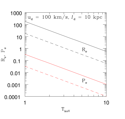
Figure 1.: Reynolds number, $R_{e}$, (upper, black lines) and Peclet number, $P_{e}$, (lower, red lines) assuming Braginskii viscosity and Spitzer conductivity. Densities are $n=10^{-2}~{}{\rm cm}^{-3}$ (solid) and $n=10^{-3}~{}{\rm cm}^{-3}$ (dashed).

The importance of viscosity is measured by the relative size of the inertial to the viscous terms in eq. 13; that is, by the Reynolds number, $R_{e}=u_{d}\ell_{d}/\nu$. When $R_{e}\gg 1$ inviscid dynamics is a good approximation. The Reynolds number must also be large for turbulence to be established for scales, $\ell_{d}$ and $u_{d}$. As for thermal conduction, it has been pointed out that Coulomb (Braginskii) viscosity can sometimes be too large in the ICM to assume these limits (e.g., Reynolds et al. 2005). Here

$$R_{e}\approx 18u_{d,100}\ell_{d,kpc}n_{-2}T_{keV}^{-5/2}.$$ (19)

$R_{e}$ and $P_{e}$ are related by the Prandtl number, $P_{r}=P_{e}/R_{e}\approx 0.08(m_{e}/m_{p})^{1/2}$, reflecting the ion diffusion and electron diffusion origins for viscosity and thermal conduction.

Fig 1. illustrates the Braginskii expression for $R_{e}$. As before, in cooler, denser ICM environments this estimate often gives $R_{e}\gg 1$, whereas in hotter rarefied ICMs that is not the case. One would have to reduce the viscosity two orders of magnitude below the Braginskii value to establish $\leq 100$ km/s turbulence on 10 kpc scales if $T_{keV}=5$ and $n_{-2}=0.1$, for instance. However, if turbulence is somehow established down to scales below $\ell_{c}(Coulomb)$, perhaps initially aided by plasma processes, the effective particle streaming lengths may become small compared to $\ell_{c}$, allowing the large $R_{e}$ needed for turbulent conditions to be maintained. Given observations that suggest turbulence in ICMs on scales of a few kpc and recognizing that radio halos may depend on turbulent cosmic ray reacceleration from small eddies Brunetti & Lazarian (2007) it is perhaps reasonable to apply inviscid MHD on those scales. We may hope that ultimate clarification of this issue will come from definitive measures of turbulence in a wide variety of ICM settings, especially on the smallest detectable scales.

4. MHD influences on AGN/ICM interactions

I assume thus, with some reservations, quasi-ideal versions of eqs. 12-15. Our primary interest, in any case, is the dynamical influence of the field, as expressed by the Lorentz force term in eq. 13. The standard criterion for evaluating its importance is to compare the magnetic pressure portion of the Lorentz force to the gas pressure gradient, so that magnetic effects are assumed small whenever $\beta>>1$. In the ICM we have $\beta\approx 400n_{-2}T_{keV}/B_{\mu G}^{2}$. Using this criterion alone we would conclude that Maxwell stresses in the ICM were unimportant. That is probably a false impression, however.

While a meaningful rule of thumb, the simple $\beta$ metric overlooks important details. A particularly simple one is that the magnetic and gas pressure forces depend on $\ell_{B}$ and $\ell_{P}$, the spatial variation scales for B and P. These scales need not be the same, especially in a complex, mostly incompressible, turbulent setting. Then, when $\beta>>1$, the magnetic field, being tangled and intermittent in magnitude, may exert a force that is much stronger than one would anticipate from a simple evaluation of $\beta$. A better metric would be $\beta(\ell_{B}/\ell_{P})\gg 1$. This point has been made by O’Neill et al. (2007) in a 3D MHD simulation study of AGN jets in an ICM containing a tangled magnetic field. Even for a mean $\beta\sim 100$, they found that the ICM magnetic field had a very significant influence on the subsonic expansion of the jet/ICM contact discontinuity, because local values of $\beta$ varied by factors of several on scales that were much smaller than the relatively smooth ICM gas pressure. Consequently magnetic pressure gradients were, in fact, sometimes comparable to gas pressure gradients.

A second point is that the magnetic tension force, which resists bending of field lines, is often more important than the pressure force, especially in subsonic flows characteristic of ICMs and many of their interfaces with AGN outflow residues. An example setting where this applies, mentioned in §2, is MHD turbulence, where magnetic tension distorts small scale eddies. The role of magnetic tension can be estimated by comparing the Maxwell stress in eq. 13 to the inertial, shear stress. From this we establish that magnetic tension may be important when $v_{A}\geq u_{d}(\ell_{B}/\ell_{d})$. If $\ell_{B}\sim\ell_{d}$, as is the case parallel to the field in MHD turbulence, we recover the $v_{A}\geq u$ criterion from §2. Other examples will be discussed below.

Another point to keep in mind, of course, is the possibility of magnetic field amplification, described by the induction eq. 13. Outside reconnection regions where dissipation is clearly important, the ideal MHD evolution of the field expressed in eq. 13 consists of field compression and field line stretching. In complex flows field line stretching is usually a bigger effect, since it is limited only by the eventual backreaction of magnetic tension and local reconnection when field lines “cross”. For incompressible flow the ideal version of eq. 13 reduces to $|B|=|B_{0}|\ell/\ell_{0}$, where $\ell$ measures the length of a field line segment. Thus, the field intensity is proportional to the stretching of the line. This will vary stochastically in a turbulent flow, leading to spatially intermittent field intensities. The constraint imposed by magnetic tension, $v_{A}<u$, on the other hand, assures that amplification of the magnetic field will be limited to magnetic pressures, $P_{B}=(1/2)v_{A}^{2}\rho$, less than the turbulent, kinetic pressure, $P_{k}\sim u^{2}\rho$.

One very important ICM MHD concern is the evolution of hydrodynamical instabilities, particularly the Kelvin-Helmholtz (K-H) and Rayleigh-Taylor (R-T) instabilities. These are both essentially incompressible instabilities that occur along boundaries such as the contact discontinuities separating AGN jet cocoons from the ICM or relic radio bubbles from the ICM. Related, R-T-like instabilities can develop anywhere equilibrium pressure and density gradients take opposite signs, or equivalently where pressure and entropy gradients have the same sign. It turns out that surprisingly weak magnetic fields can significantly modify these instabilities, sometimes quenching them and sometimes controlling their nonlinear evolution even when magnetic stresses do not prevent the instabilities from developing.

The K-H instability develops hydrodynamically along a shear layer for wavelengths exceeding the shear layer thickness, provided the shear velocity is not highly supersonic. Tension from a magnetic field component parallel to the velocity in the shear layer and aligned with the wavevector of a perturbation will resist growth of the instability, since growing oscillations lengthen the boundary. For a velocity discontinuity, $\Delta u$, separating fluids of equal density the linear growth rate of a small perturbation with wavenumber k is Chandrasehkar (1961)

$$\Gamma=(1/2)k\Delta u\sqrt{(1-4v_{A,||}^{2}/\Delta u^{2})}.$$ (20)

The perturbation is stable ($\Gamma^{2}<0$) for $v_{A,||}\geq\Delta u/2$. Linear stabilization of the K-H instability in the ICM would roughly require $B_{\mu G}>2u_{d,100}n_{-2}^{1/2}$, a condition that is likely to be met along interfaces of low density and modest velocity contrast, as pointed out, for example, by De Young (2003).

It is important to realize, however, even when it is initially much too weak to inhibit the linear K-H instability, that a magnetic field can play a very important role in the nonlinear K-H instability. This influence results from stretching (amplification) of the initial field within the unstable flow. For example, Ryu et al. (2000) carried out 3D MHD simulations of K-H unstable flows, and found that even for initial conditions with $v_{A,||}\sim 0.02\Delta u$, the unstable flow evolved into a relaxed, laminar form with aligned, self-organized magnetic and velocity fields, contrary to the turbulent velocity field that developed in the absence of a magnetic field. The key insight is that the 3D hydrodynamical flow initially forms into line vortices along the unstable slip surface, stretching the magnetic field across each vortex. Subsequently, the vortex is unstable in 3D to so-called rib vortices transverse to the main vortex. This greatly adds to the net stretching of the field, making it possible locally and temporarily that $v_{A}>\Delta u$ and, thus for an initially weak field to alter evolution of the flow.

The linear R-T instability is influenced by a magnetic field parallel to a density discontinuity in a way similar to the K-H instability; magnetic tension resists the stretching of the boundary. Defining the density jump across the discontinuity as $r=\rho_{2}/\rho_{1}$, where region ‘2’ is on top with respect to gravity, g, and letting $\tilde{v}_{A}^{2}=B^{2}/[4\pi(\rho_{1}+\rho_{2})]$, the growth rate is Chandrasehkar (1961)

$$\Gamma=\sqrt{[1/(r+1)]}\sqrt{[gk(r-1)-2\tilde{v}_{A,||}^{2}k^{2}]}.$$ (21)

In this case the influence of the magnetic tension depends on wavelength, so that the instability is suppressed when $k>k_{0}=(1/2)g(r-1)/[\tilde{v}_{A,||}^{2}(r+1)]$, while there is a maximum linear growth rate at wavenumber, $k_{max}=(1/2)k_{0}$, given by

$$\Gamma_{max}=(1/2\sqrt{2})g(r-1)/[\tilde{v}_{A,||}(r+1)].$$ (22)

As a mnemonic, imagine for a large density contrast, $r\gg 1$, that the free fall over a time $\sim 1/\Gamma_{max}$ reaches a velocity $\sim\tilde{v}_{A,||}$, and a length $\sim 1/k_{max}$. It turns out even a vertical magnetic field reduces linear growth of the R-T instability, although it does not totally quench it. The asymptotic short wavelength growth rate is of order $g/v_{A}$, compared to the hydrodynamical rate $\sim\sqrt{gk}$. These two rates are similar for $k\sim g/v_{A}^{2}$, mirroring the horizontal field behavior. As a rule of thumb, then, we can expect magnetic inhibition of the R-T instability whenever the Alfvén speed is greater than or comparable to $\sqrt{g\ell}$. That would correspond roughly to a magnetic field $B_{\mu G}\geq 7((n_{-2}~{}g_{-7}\ell_{d.kpc})^{1/2}$, where $g_{-7}$ is the gravitational acceleration in units of $10^{-7}~{}{\rm cm/s^{-2}}$. Alternatively one could view this relation to indicate, given ICM magnetic fields of order a microGauss, that R-T instabilities on scales smaller than a few kpc are likely to be inhibited. As I noted earlier and others have also emphasized (e.g., Reynolds et al. 2005), viscous effects on this scale could also be important, depending on how much plasma and magnetic fields reduce the effective free-streaming length for protons. Which influence, magnetic tension or viscosity, is dynamically more important on this scale remains to be established (e.g., Kaiser et al. 2005).

Ideal MHD influences in the nonlinear R-T instability are a bit complicated, as pointed out by Jun et al. (1995) in a 2D and 3D simulation study of the nonlinear MHD R-T instability. The nonlinear hydrodynamic R-T instability is characterized by the formation of dense fingers that ‘drip’ downward and light “bubbles” that rise. These eventually lead to turbulent conditions. Jun et al. noted that the vertical component of B aligned with gravity eventually dominates the evolution of these structures, especially when the initial field is only moderately weaker than needed to suppress the linear instability. Then, in fact, since the vertical magnetic field aligns with the edges of R-T fingers, it inhibits development of a secondary R-T instability that otherwise disrupts those fingers. Thus, it can actually enhance their early development. Ultimately, however, even a relatively weak magnetic field caught up in the nonlinear development of the R-T instability can be amplified through stretching to restrict growth of turbulent behaviors.

There are a limited number of MHD simulation studies of AGN and/or radio relic, bubble interactions with ICMs. They generally support the points made here, including the realization that fields at least several times weaker than those expected by the usual metrics can play essential dynamical roles. As examples, Robinson et al. (2004) and Jones & De Young (2005) considered 2D MHD buoyant bubbles in model ICMs with large scale magnetic fields, pointing out that even when $\beta\gg 1$ field stretching could stabilize boundaries that otherwise were disrupted by R-T and K-H instabilities. De Young et al. (2007) obtained similar results for 3D bubbles, but also noted that since field line tension acts only in the plane containing the field and its curvature, the bubbles remained subject to disruption along lines orthogonal to the field-gravity plane. Ruszkowski et al. (2007) carried out 3D MHD bubble simulations in which the ICM magnetic field was tangled. They noted that when the outer tangling scale was smaller than the size of the bubble the magnetic field was no longer effective in stabilizing the bubbles. This result, confirmed by De Young et al. (2007), reflects the fact that disruption comes from instabilities on the scale of the bubble. It is obvious that magnetic tension, the primary MHD stabilizing influence, does not operate on scales greater than the coherence length of the field. On those scales we should expect the dynamics to be largely hydrodynamic, except for magnetic pressure gradient effects. I already mentioned that O’Neill et al. (2007) pointed out how variations in magnetic pressure on scales smaller than gas pressure variations can produce important dynamical consequences even when $\beta\gg 1$.

5. Conclusion

As a number of previous authors have discussed, Coulomb mean free paths in the ICM can sometimes be uncomfortably large when one wants to model the ICM as an ideal fluid. Yet observed features, such as shocks, sharp contact discontinuities and turbulence strongly suggest continuum, fluid behaviors. It seems likely that a combination of plasma instabilities and magnetic field influences reduce the effective particle free-streaming lengths enough to allow relatively inviscid, fluid-like behaviors at least beyond kiloparsec scales. Whether these effects can also reduce diffusion rates of electrons sufficiently to effectively quench thermal conduction is less certain. In any case electrical conductivity is very likely to be sufficient to apply a frozen-in magnetic field model on these scales.

Even though magnetic pressures in the ICM are likely to be much smaller than gas pressures, magnetic fields there can still play a significant dynamical role. This is especially because the local Alfvén velocity can be comparable to or exceed local flow speeds, since ICM flows are usually subsonic. In that case magnetic tension forces can compete with dynamical stresses. This probably influences ICM turbulence on small, say kiloparsec, scales and helps stabilize flows that are otherwise hydrodynamically unstable.

Acknowledgments.

This work was supported in part by NSF grant AST 06-07674 to the University of Minnesota and by the Minnesota Supercomputing Institute. I am grateful to a number of collaborators over the years who contributed insights and results that have gone into this review, especially Dave De Young, Adam Frank, Francesco Miniati, Sean O’Neill and Dongsu Ryu.

References

- Beck et al. (2006) Beck, R., Brunetti, G. & Feretti, L. 2006, Astron. Nachr., 327, 385
- Bertschinger & Meiksin (1986) Bertschinger, E. & Meiksin, A. 1986, Ap. J., 306, L1
- Boyd & Sanderson (2003) Boyd, T. J. M. & Sanderson, J. J. 2003, The Physics of Plasmas (Cambridge: Cambridge University Press)
- Braginksii (1965) Braginskii, S. I. 1965, Rev. Plasma Phys., 1, 205
- Brunetti & Lazarian (2007) Brunetti, G. & Lazarian, A. 2007, M. N. R. A. S., 378, 245
- Carilli & Taylor (2002) Carilli, C. L. & Taylor, G. B. 2002, A.R.A.A., 40, 319
- Chandrasehkar (1961) Chandrasekhar, S. 1961, Hydrodynamic and Hydromagnetic Stability (London: Oxford University Press)
- Croston et al. (2005) Croston J. H., Hardcastle, M. J., Harris, D. E., Belsole, E., Birkinshaw, M. & Worrall, D. M. 2005, Ap.J., 626, 733
- De Young (2003) De Young, D. S. 2003, M. R. A. S., 343, 719
- De Young et al. (2007) De Young, D. S., O’Neill, S. M. & Jones, T. W. 2007 (in preparation)
- Dolag (2006) Dolag, K. 2006, Astron. Nachr., 327, 575
- Fabian et al. (2005) Fabian, A. C., Reynolds, C. S., Taylor, G. B. & Dunn, R. J. H. 2005, M. N. R. A. S., 363, 891
- Goedbloed & Poedts (2004) Goedbloed, H. & Poedts, S. 2004, Principles of Magnetohydrodynamics (Cambridge: Cambridge University Press)
- Gruzinov (2002) Gruzinov, A. 2002, arXiv:astro-ph/0203031
- Gruzinov (2006) Gruzinov, A. 2006, arXiv:astro-ph/0611243
- Hall (1980) Hall, A. N. 1980, M. N. R. A. S., 190, 353
- Jones & De Young (2005) Jones, T. W. & De Young, D. S. 2005, Ap. J., 624, 586
- Jun et al. (1995) Jun, B.-I., Norman, M. L. & Stone, J. M. 1995, Ap. J., 453, 332
- Kaiser et al. (2005) Kaiser, C. R., Pavlovski, G., Pope, E. C. D. & Fangohr, H. 2005, M. N. R. A. S., 359, 493
- Kronberg (1996) Kronberg, P. P. 1996, Space Sci. Rev., 75, 387
- Kulsrud (2004) Kulsrud, R. M. 2004, Plasma Physics for Astrophysics (Princeton: Princeton University Press)
- Lazarian (2007) Lazarian, A. 2007, arXiv:0707.0702
- Narayan & Medvedev (2001) Narayan, R. & Medvedev, M. V. 2001, Ap.J. Lett., 562, L129
- O’Neill et al. (2007) O’Neill, S. M., Jones, T. W. & Ryu, D. 2007 (in preparation)
- Pope et al. (2005) Pope, E. C. D.,Pavlovski, G., Kaiser, C. R. & Fangohr, H. 2005, M. N. R. A. S., 364, 13
- Priest & Forbes (2000) Priest, E. & Forbes, T. 2000, Magnetic Reconnection: MHD Theory and Its Applications (Cambridge: Cambridge University Press)
- Reynolds et al. (2005) Reynolds, C. S., McKernan, B., Fabian, A. C., Stone, J. M. & Vernaleo J. C. 2005, M. N. R. A. S., 357, 242
- Robinson et al. (2004) Robinson, K., et al. 2004, Ap. J., 601, 621
- Ruszkowski et al. (2007) Ruszkowski, M., Ensslin, T. A., Brueggen, M., Heinz, S. & Pfrommer, C. 2007, M. N. R. A. S., 378, 662
- Ryu et al. (2000) Ryu, D., Jones, T. W. & Frank, A. 2000, A. J., 545, 475
- Ryu et al. (2007) Ryu, D., Kang, H., Cho, J. & Das S. 2007, (in preparation)
- Schekochihin et al. (2005) Schekochihin, A. A., Cowley, S. C., Kulsrud, R. M., Hammett, G. W. & Sharma, P. 2005, Ap.J., 629, 139
- Schuecker et al. (2004) Schuecker, P., Finoguenov, A., Miniati, F., Boehringer, H. & Briel, U. G. 2004, A&A, 426, 387
- Spitzer (1962) Spitzer, L. 1962, Physics of Fully Ionized Gases (New York: Interscience Publishers)
- Stix (1992) Stix, T. H. 1992, Waves in Plasmas (New York: AIP)
- Vikhlinin et al. (2001) Vikhlinin, A., Markevitch, M. & Murray, S. S. 2001, Ap.J. Lett., 549, L47
- Worrall & Birkinshaw (2000) Worrall, D. M. & Birkinshaw, M. 2000, Ap.J., 530, 719