The study of a new gerrymandering methodology 111Supported by our deep interests in mathematical modeling.
Abstract
This paper is to obtain a simple dividing-diagram of the congressional districts, where the only limit is that each district should contain the same population if possibly. In order to solve this problem, we introduce three different standards of the ”simple” shape. The first standard is that the final shape of the congressional districts should be of a simplest figure and we apply a modified ”shortest split line algorithm” where the factor of the same population is considered only. The second standard is that the gerrymandering should ensure the integrity of the current administrative area as the convenience for management. Thus we combine the factor of the administrative area with the first standard, and generate an improved model resulting in the new diagram in which the perimeters of the districts are along the boundaries of some current counties. Moreover, the gerrymandering should consider the geographic features.The third standard is introduced to describe this situation. Finally, it can be proved that the difference between the supporting ratio of a certain party in each district and the average supporting ratio of that particular party in the whole state obeys the Chi-square distribution approximately. Consequently, we can obtain an archetypal formula to check whether the gerrymandering we propose is fair.
1 Introduction

To ensure the fairness of the election, the foremost task is to obtain a scientific arrangement of the boundaries of the congressional districts. Although the states constitution provides the number of representatives each state may have, it articulates nothing about how the district shall be determined geographically.
This oversight has nowadays led to an unnatural district shape which includes many long and narrow areas. Taking the state of New York as an example, on the map of current congressional districts[2], we can see that there are some unnatural-shaped districts, such as districts 20th and 22nd (shown in Figure 12(a)). To create the “simplest” shapes, where the only limit is that each district should contain the same population if possibly, we introduce three different standards of the simplicity:
-
1.
Each district is approximatively a rectangle.
-
2.
Based on the above standard, the outlines are best along the boundaries of counties.
-
3.
The modifications of geographical features and fairness are combined in the final model.
Therefore, we should take into accounts comprehensive factors including the population, the boundaries of counties, geographic features and fairness when gerrymandering.
1.1 Issues in the Model
-
•
The first objective is to divide the state into some districts following the rule that the population of each district must be same.
-
•
As the second objective, we wish to make the boundaries of the districts as simple as possible according to the 1st standard we have proposed above.
-
•
The third objective is that we need further modifications considering the standard 2 and standard 3.
1.2 Previous Works
There are many existing methods to realize the gerrymandering, with the consideration of different aspects. For instance, the “shortest split line algorithm”[3] considers the simplicity of the shape as key factors. Another method, which uses the statistical physics approach, takes every county as a single element of a matrix, makes an analogue to the q-state pots[7] model, and gets the optimal solution keeping the integrality of a county. Other approaches such as the “fixed district algorithm”[3] and the “changing the voting system method”[3] mainly consider the unbiasedness of the election as the crucial factor.
In our work, the foremost task is to make sure the simplicity of the shapes of districts. Therefore, we modify the “shortest split line algorithm” to establish our initial simple model. The main modification is that we only use horizontal line and vertical line instead of diagonals. In this way, we can get simple rectangles other than irregular polygonal districts. While in the section of Model Modification we develop a new method to ensure the perimeter of the districts are along the boundaries of the current counties.
1.3 Our Approach
-
•
First, we obtain the population density matrix from the density map.
-
•
In order to obtain a simple shape of districts, we only take into account the rule that every district should have the same population to establish a simple model.
-
•
Then we optimize our model by adding the modification of the present shapes of counties and gain a more nature looking figure.
-
•
Based on the results from the forgoing simulation, we finally investigate into the factor of geography and fairness in detail when gerrymandering.
1.4 Our Result
According to the steps mentioned above, Figure 1 shows our results when applying our model to the state of New York.
2 Basic Gerrymandering Model
In order to establish our basic model, we first obtain a population density matrix using the population map. We then establish a simple model with the only constraint being that each district have the same population. Finally, we optimize our model by adding additional constraints such as preventing the division of original administrative areas.
2.1 Acquirement of the Population Density Matrix
To calculate the population each district contains, we must first extract the population density matrix for later computer programming from the existing census data of some big cities and the macroscopic population density map.
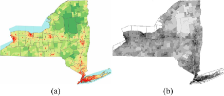
For the original colored population map, we use Matlab to identify the color of every pixel. Thus we can get the population density corresponding to the particular pixel though which we obtain the population density matrix. Moreover, this matrix can be shown as a grey level figure(Figure 2).
2.2 A Simple Model for Redistricting
In order to obtain simple shapes for congressional districts, we modified the original “shortest split line algorithm” and developed a simple algorithm to divide districts. In our model:
-
•
We focus on keeping an even distribution of population in each district, ignoring other factors.
-
•
The algorithm takes as input only the population density matrix and ignores other factors such as party loyalties of the citizens, thus guaranteeing unbiased results.
-
•
We use horizontal and vertical lines to separate the state result in fairly rectangle districts.
The procedure of the algorithm can be shown in Figure 3.
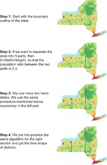
This district-dividing algorithm has the advantage of simplicity, clear unbiasedness, and it produces fairly nice-looking rectangle districts.
The advantages of the simple model:
-
•
Simplicity
-
•
Clear unbiasedness
-
•
Fairly nice-looking rectangle districts.
The disadvantages:
-
•
Fails to take into consideration other factors such as geographic features and integrality of the counties.
2.3 Model Modification
Despite of its advantage of simplicity, the original model has the disadvantage of ignoring the shape of administrative area and geographic features. As the figures show, the boundaries produced by the original algorithm some times divide a county which is an administrative area into different parts. This can prove inconvenient and unnatural when carrying out the election procedures. To dispel this disadvantage, we made the following improvements to our original model:
2.3.1 A Basic Assumption
Before taking into consideration additional factors in dividing the counties, we need to make the following assumption: we assume that two districts share approximately the same population if the difference in their numbers of voters is no more than .
In reality, it is impossible to divide districts into absolutely equal numbers of voters due to the influence of population flow and the fluctuation of birth and death rates. And most of the constitutions also allow the the standard deviation of number of voters to fall within .
2.3.2 Modification Method
After making up the designs of landform, we are faced with a problem - how to adopt the borderline to avoid dividing up administrative districts. To solve this problem, we have to adopt the borderlines between the administrative districts. We follow the lines in bulge and concave in some district. As we think the density in population almost equals close to borderline between districts. Taking into account the factors of population, landform and management, we take this division as a simple meaning in management.
2.3.3 Our Algorithm
The basic consideration of this improved model is the same with the above simple model. However, in that model, the dividing lines are all straight and thus cannot keep a single county integrate. Now we are trying to overcome this shortcoming and do our best to make the dividing line coincide with the boundary of each administrative area, although county dividing is unavoidable.
Step 1:
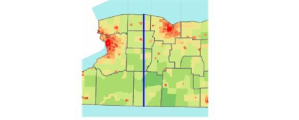
Use the simple model to find the straight dividing line.
Step 2:
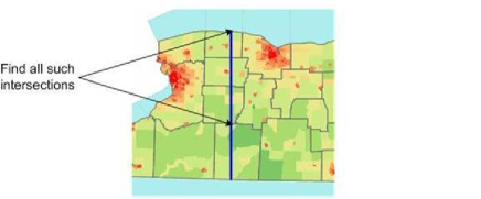
Find all the intersections between the straight line and the county boundaries. Then in the program, use “count” the integer to represent how many crossover points there are on the straight line and use array point[count] to record the location of all these intersections.
Step 3:
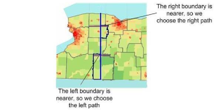
There must be 2 or 3 direct paths along the straight line or the boundary of the county the straight line goes through connecting the two intersection points. We are trying to decide which of the two paths along the boundary is more “simple”. The “simple” path should be the boundary which connects the adjoining points and more close to the straight line.
First we find the point on the straight line whose coordinate position is 2 or 3 units away from the intersection. We separately search the points left and right to it (take vertical line as an example, for horizontal lines the 2 directions would be above and below). The direction we finally choose would be the one on which we arrive at the boundary earlier. We record the direction chosen in array path[count-1], if the direction is left or upward, path[i]=1, if it is right or downward, path[i]=3.
This method may not be very strict, but it is easy to realize and takes very little time for the computer to execute.
Step 4:
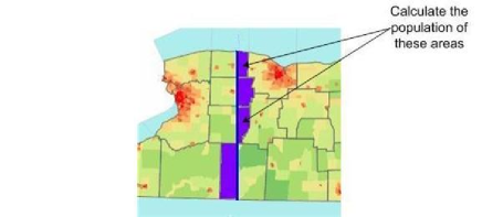
Every straight line between two adjoining points and the boundary line chosen in step 3 can confine a small area. We calculate the population in each small area by sum up the elements of the population density matrix including in the area. Pay attention that if the area is to the left or below the straight line, prescribe that s[i] is negative, otherwise, it is positive. We save the result in array s[count-1].
Step 5:
In this step we will finally decide the dividing line - its shape and location. We now know all the points on the dividing line and want to decide the lines joining the points. We use array path[count-1] to describe these lines. path[i] stands for the line connecting the ith point and the (i+1)th point. path[i] =1,2,3 stands for the , , path count from left to right or downwards to upwards.
The principles we use to decide which path to choose is like this:
First, while we replace the initial straight line with the boundary line, the population of different congressional districts will vary to each other. So the differences must be controlled within a certain range.
Second, we should use as little as possible straight lines, because choosing a straight path means one county will be divided into two.
The method is as follows:
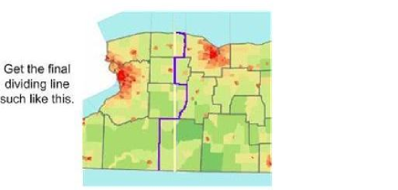
In step 4 we get the array s[count-1], we first sum up all the elements in s[count-1] and get the result S. Judge whether , here, delta can be the theoretical population of a congressional district multiple with the allowed range of error (in our program we choose the range as ), if so, we consider current path is qualified and we get the final array path[count-1], exit loop; if not, we find s[i] which is closest to S ( is the minimum), and let path[i]=2 (change the path to the straight line) let , return to judge whether , … ,and loop like this.
After exiting the loop, print the location of the initial straight line and its end points, point[count] and path[count-1].
The final dividing line we get with this method may not be the optimal line, but it is qualified. The method can avoid considering all the possible combination of paths and thus can operate very fast.
Step 6: Do the recursion as the simple model and get all the dividing line.
3 Further Optimization of the Model
Except shape and county integrity, other factors should also be taken into account in actual gerrymandering. For example, how to avoid biased “gerrymandering , how to modify our model in special landform, as we are going to represent.
3.1 The Modification of Avoiding “Gerrymandering”
3.1.1 Brief Introduction
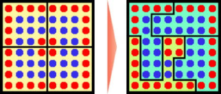
There are two principal strategies behind gerrymandering[3,8]: maximizing the effective votes of supporters, and minimizing the effective votes of opponents. One form of gerrymandering, packing is to place as many voters of one type into a single district to reduce their influence in other districts. A second form, cracking, involves spreading out voters of a particular type among many districts in order to reduce their representation by denying them a sufficiently large voting block in any particular district. The methods are typically combined, creating a few “forfeit” seats for packed voters of one type in order to secure even greater representation for voters of another type.
3.1.2 Resolution
Because the simple algorithm we based on uses only the shape of the state, the number m of districts wanted, and the population distribution as inputs - and does not know the party loyalties of the voters in any given region - the result cannot be biased[3,9].
However we can not completely prevent the certain voter biases from occurring due to the random redistricting process - although the probability is small. As a result, we need make a mathematical analysis to determine whether the gerrymandering our model proposed is fair.
-
•
Model assumption:
Due to the the influence of population flow and the fluctuation of birth, death and the supporting ratio of a political party. It is reasonable to assume that the supporting ratio of a particular party in each district is incorrelate of one another approximately. Next we would analyze how to judge the fairness of the gerrymandering to a specific party (Republican in our example) ; other parties and situations can be judged via the same method.
-
•
Mathematical Analysis:
| (1) |
If represents the supporting ratio of the Republican in district and this district has n voters, then we would expect to get (3.2)
| (2) |
Let p be the last-few-year average supporting ratio of the Republican in the whole state. Thus we can expect that
| (3) |
Obviously, is distributed by B(1,p).
| (4) | |||||
According to the statistics theory, obeys N(0,1), if n is large enough.
Then it is reasonable to obtain the following deduction:
| (5) |
Here m indicates the number of districts in a certain state. Thus, we can use Equ.(3.5) to generate a simple but effective standard to judge the fairness of the original gerrymandering.
According to the statistics theory, if we get the population density of the supporting ratio of the Republican, it is easy to gain using the data and p.
After that, the foremost task is to determine a parameter scientifically. The parameter functions as a threshold to judge whether the current gerrymandering is bias or not. Then from the data table of distribution , we can get the value where . Here stands for the random variable distributed by .
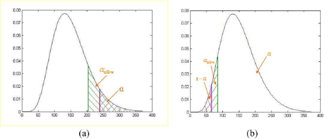
On one hand, if there happens the “packing” situation, we would expect to be extremely small. Therefore, if , we can judge this gerrymandering as packing situation leading to unfairness. On the other hand, if “cracking” situation happens, we can expect to be extremely small. We consider this gerrymandering biased as the same (shown in Figure 10).
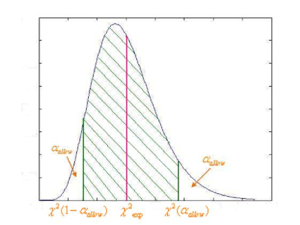
In conclusion, if the gerrymandering is fair, the value of produced by it would comply with following limits.
| (6) |
We can briefly obtain the final limit on value (shown in Figure 11), that is
| (7) |
-
•
Conclusion:
After generating the “simple” congressional districts, we can use Equ.(3.5) and (3.7) to judge whether it satisfies the requirement of fairness, if we can collect the supporting ratio of the Republican in each district, the last-few-year average supporting ratio in the whole state and the parameter . If it is not a fair gerrymandering, we need to reconsider the procedure of redistricting.
3.2 The Modification of Geographic Features
Up till now, many models that can realize gerrymandering have existed. Thus comparison between all kinds of gerrymandering results is necessary. We are going to further analysis the characteristic of our two models while comparing the results we get with others.
3.2.1 Brief Introduction
Above-mentioned method has ignored landform factors such as main rivers, mountains, lakes in process of choosing partition, thus it has made district partition unnatural. Here we make some improvements.
As to main rivers, mountains and so on, we hold the view that along the river, population benefit in economy comparatively resembles. On this basis, the areas on the river should be one district.
3.2.2 Resolution
Our operations are as follows:
-
1.
A new district with a large population is based on expanding along the river and mountains. Considering the advantages of the long river or deep mountains, as well as convenience in management, more districts will be formed if the population increases.
-
2.
To the large lake, we expand the area into several districts along the bank, for they are blessed with the same interest in economy.
-
3.
To the area of mountains and plain, we consider developing them separately as a result of different demands in benefit.
-
4.
The same thinking is practical along the coastline. We assemble people on the coast into several districts, to separate the areas of coastline from inland to help the development from the coastline to the inland.
-
5.
Considering the approaching interest in economy, the area of islands and bylands is being considered alone. A special zone will be built.
With these factors of landform being considered alone, priority to every electoral district deducted, to the part remaining again, we will carry out the previous simple operation according to the simple model.
4 Conclusion and Analysis
4.1 Comparison of Our Two Models
We have fully established two models - the simple one and the refined one, both of which are easy to realize. Each of these two models has its own prominent advantages.
As to the simple model, first of all, the final shapes of the congressional districts are all very simple, constructing with horizontal and vertical lines only. Moreover, the simple model guarantees that each district contains the same population if given a precise population division.
While to the refined model, we can maintain the integrity of every single county to a large extent, which ease the management of actual voting. What s more, although the population of districts varies from each other, the differences can be controlled theoretically to any proposed precision.
4.2 Comparison With Other Models
There are many existing methods to realize the gerrymandering with the consideration of different aspects. Here we compares our model with the “shortest split line algorithm” and the “q-state pots model”.
From the theoretically analysis and the final result, we can see that our method has its merits.
First, one important task for us is to make sure the simplicity of the shapes of districts. Therefore, we modify the “shortest split line algorithm” to establish our initial simple model. The main modification is that we only use horizontal line and vertical line instead of diagonals. In this way, we can get simple rectangles other than irregular polygonal districts produced by original “shortest split line algorithm”.
Secondly, we think the “q-state potts model” is excellent. The foremost characteristic of it is that this model keeps the integrity of counties. However, the difference of district populations can just be controlled within , while this difference in our model is no more than .
In sum, the advantages of our model is that:
-
1.
Easy to carry out in the computer.
-
2.
Simple shapes of the districts.
-
3.
Combined with the factor of avoiding dividing up the current administrative ares.
-
4.
The difference of district populations can be controlled in any precision.
4.3 Comparison With Current Districts
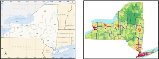
From Figure 12, we can clearly see the difference between the current (the left one) districts and the redistricting proposed by our model. Through careful comparison, we can draw the conclusion that each has its advantages.
The current shape of districts own its great merit that it take into the geographical consideration. For example, the district is built along the Lake Ontario and the district mainly consists of plain. Both show the modification of geographic features.
Although there is some merit in the current district, the gerrymandering result produced by our model still show its advantages.
-
1.
The shape of most districts are rectangular satisfying the retirements of the “simplicity”.
-
2.
Most of the perimeters of the district are along the boundaries of current counties resulting in the convenience of management.
-
3.
Last but not least, the difference of district populations is no more than , and can be controlled in any precision.
Finally, we have generated a simple but effective criterion to judge the fairness of the gerrymandering via the reasonably mathematical analysis which makes the model as a whole.
5 Weakness and Further Development
Although our two models are reasonable and easy to realize, the final gerrymandering model still have some weakness which needs further improvement.
5.1 Verification of the Improved Model
Although we have implemented the improved model to take into consideration the fairness of voter distribution by party, we cannot obtain the data on population density favoring respective parities or on supporting ratio of a specific party. Therefore we can not put that part of the model into practice. In another word, if we want to prove the effectiveness and fairness of the model we should try our best to investigate such data and further correct our simulations and mathematical analysis.
5.2 Realization of the Comprehensive Considerations
Although we have noticed the importance of geographic features when gerrymandering, due to the complexity of our current model considering another key factor - avoiding separating administrative areas, we have not achieved the goal that programs the algorithm considering the landform modification. Therefore, our next mission is to realize the comprehensive considerations including geographic factors.
6 Appendix
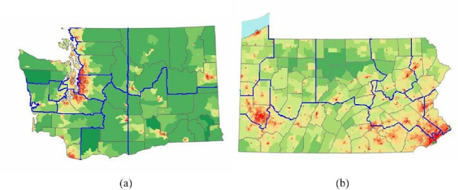
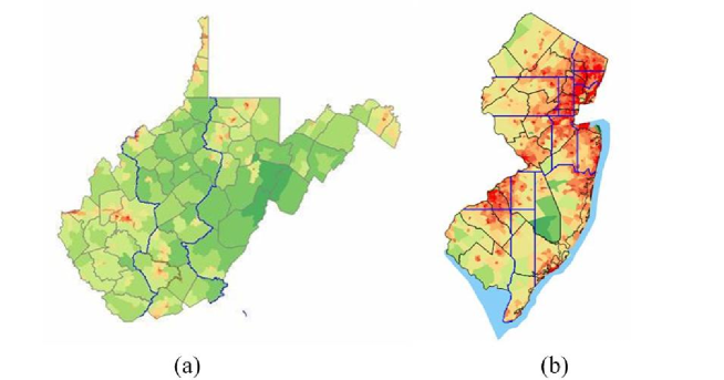
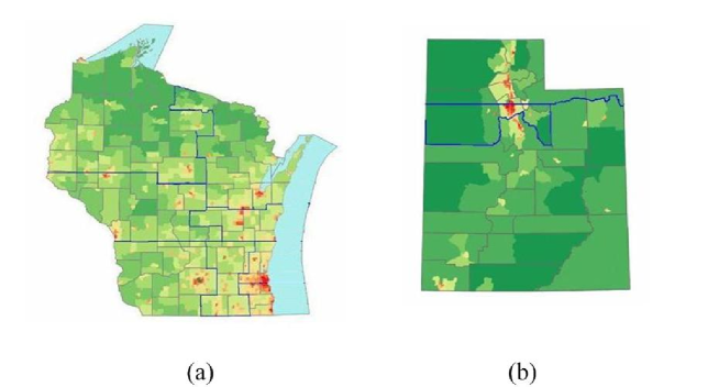
Applications to Other States
References
- [1] Population density maps of all the states, http://www.answers.com, Accessed Feb 10th, 2007
- [2] Current congressional districts of all the states, http://www.census.gov, Accessed Feb 10th, 2007
-
[3]
Gerrymandering - Wikipedia, the free encyclopedia,
http://en.wikipedia.org/wiki/Gerrymandering, Accessed Feb 9th, 2007 -
[4]
Cognitive Aspects of Gerrymandering,
http://www.springerlink.com/index,
Accessed Feb 10th, 2007 -
[5]
Population list of all the counties in the state of New York,
http://www.citypopulation,de/USA-New York.html, Accessed Feb
9th, 2007 -
[6]
Current congressional districts of all the states,
http://nationalatlas.gov/printable/congress.html, Accessed Feb 11st, 2007 -
[7]
Huntington News,
http://www.huntingtonnews.net/national/061006-shns-elections.html,
Accessed Feb 11st, 2007 - [8] FairVote - Fairness and Independence in Redistricting Act (H.R. 2642), http://www.fairvote.org, Accessed Feb 10th, 2007
-
[9]
Partisan Gerrymandering,
http://www.senate.leg.state.mn.us/departments/scr/redist/red2000/ch5parti.htm, Accessed Feb 10th, 2007 - [10] Range voting, http://www.rangevoting.org, Accessed Feb 10th, 2007
- [11] The theory of statistics, http://www.statistics.gov, Accessed Feb 10th, 2007
- [12] Fair Vote Gerrymander Examples, http://www.westmiller.com
- [13] K Sherstyuk. “How to gerrymander: A formal analysis”, Springer, 1998
- [14] TW Gilligan, JG Matsusaka. “Structural constraints on partisan bias under the efficient gerrymander”, Springer,1999
- [15] JD Cranor, GL Crawley, RH Scheele. “The Anatomy of a Gerrymander”, American Journal of Political Science, 1989
- [16] BE Cain. “Assessing the Partisan Effects of Redistricting”, The American Political Science Review, 1985