$\mathfrak{sl}(N)$-link homology ($N\geq 4$) using foams and the Kapustin-li formula

Abstract.

We use foams to give a topological construction of a rational link homology categorifying the $\mathfrak{sl}(N)$ link invariant, for $N\geq 4$. To evaluate closed foams we use the Kapustin-Li formula adapted to foams by Khovanov and Rozansky [7]. We show that for any link our homology is isomorphic to the Khovanov-Rozansky [6] homology.

1. Introduction

In [10] Murakami, Ohtsuki and Yamada (MOY) developed a graphical calculus for the $\mathfrak{sl}(N)$ link polynomial. In [3] Khovanov categorified the $\mathfrak{sl}(3)$ polynomial using singular cobordisms between webs called foams. Mackaay and Vaz [9] generalized Khovanov’s results to obtain the universal $\mathfrak{sl}(3)$ integral link homology, following an approach similar to the one adopted by Bar-Natan [1] for the original $\mathfrak{sl}(2)$ integral Khovanov homology. In [6] Khovanov and Rozansky (KR) defined a rational link homology which categorifies the $\mathfrak{sl}(N)$ link polynomial using the theory of matrix factorizations.

In this paper we use foams, as in [1, 3, 9], for an almost completely combinatorial topological construction of a rational link homology categorifying the $\mathfrak{sl}(N)$ link polynomial. Our theory is functorial under link cobordisms. Khovanov had to modify considerably his original setting for the construction of $\mathfrak{sl}(2)$ link homology in order to produce his $\mathfrak{sl}(3)$ link homology. It required the introduction of singular cobordisms with a particular type of singularity. The jump from $\mathfrak{sl}(3)$ to $\mathfrak{sl}(N)$, for $N>3$, requires the introduction of a new type of singularity. The latter is needed for proving invariance under the third Reidemeister move. Furthermore the combinatorics involved in establishing certain identities gets much harder for arbitrary $N$. The theory of symmetric polynomials, in particular Schur polynomials, is used to handle that problem.

Our aim was to find a combinatorial topological definition of Khovanov-Rozansky link homology. Such a definition is desirable for several reasons, the main one being that it might help to find a good way to compute the Khovanov-Rozansky link homology. Unfortunately the construction that we present in this paper is not completely combinatorial. The introduction of the new singularities makes it much harder to evaluate closed foams and we do not know how to do it combinatorially. Instead we use the Kapustin-Li formula [5], adapted by Khovanov and Rozansky [7]. A positive side-effect is that it allows us to show that for any link our homology is isomorphic to Khovanov and Rozansky’s.

Although we have not completely achieved our final goal, we believe that we have made good progress towards it. In Propositions 6.2 and 6.9 we derive a small set of relations on foams which we show to be sufficient to guarantee that our link homology is homotopy invariant under the Reidemeister moves. By deriving these relations from the Kapustin-Li formula we prove that these relations are consistent. However, in order to get a purely combinatorial construction we would have to show that they are also sufficient for the evaluation of closed foams, or, equivalently, that they generate the kernel of the Kapustin-Li formula. We conjecture that this holds true, but so far our attempts to prove it have failed. It would be very interesting to have a proof of this conjecture, not just because it would show that our method is completely combinatorial, but also because our theory could then be used to prove that other constructions, using different combinatorics, representation theory or symplectic/complex geometry, give functorial link homologies equivalent to Khovanov and Rozansky’s. So far we can only conclude that any other way of evaluating closed foams which satifies the same relations as in Propositions 6.2 and 6.9 gives rise to a functorial link homology which categorifies the $\mathfrak{sl}(N)$ link polynomial. We conjecture that such a link homology is equivalent to the one presented in this paper and therefore to Khovanov and Rozansky’s.

In section 2 we recall some basic facts about the $\mathfrak{sl}(N)$-link polynomials. In section 3 we recall some basic facts about Schur polynomials and the cohomology of partial flag varieties. In section 4 we define pre-foams and their grading. In section 5 we explain the Kapustin-Li formula for evaluating closed pre-foams and compute the spheres and the theta-foams. In section 6 we derive a set of basic relations in the category $\mathbf{Foam}_{N}$, which is the quotient of the category of pre-foams by the kernel of the Kapustin-Li evaluation. In section 7 we show that our link homology complex is homotopy invariant under the Reidemeister moves. In section 8 we show that our link homology complex extends to a link homology functor. In section 9 we show that our link homology, obtained from our link homology complex using the tautological functor, categorifies the $\mathfrak{sl}(N)$-link polynomial and that it is isomorphic to the Khovanov-Rozansky link homology.

2. Graphical calculus for the $\mathfrak{sl}(N)$ polynomial

In this section we recall some facts about the graphical calculus for $\mathfrak{sl}(N)$. The $\mathfrak{sl}(N)$ link polynomial is defined by the skein relation

$$q^{N}P_{N}(\undercrossing)-q^{-N}P_{N}(\overcrossing)=(q-q^{-1})P_{N}(\orsmoothing),$$

and its value for the unknot, which we take to be equal to $[N]=(q^{N}-q^{-N})/(q-q^{-1})$. Let $D$ be a diagram of a link $L\in S^{3}$ with $n_{+}$ positive crossings and $n_{-}$ negative crossings.

$$\begin{array}[]{cclcccl}\text{positive: }\ \raisebox{-9.0pt}{\includegraphics[height=21.68121pt]{overcrossing.eps}}&=&\raisebox{-9.0pt}{\includegraphics[height=21.68121pt]{orsmoothing.eps}}-q\raisebox{-9.0pt}{\includegraphics[height=21.68121pt]{dbedge.eps}}&&\text{negative: }\ \raisebox{-9.0pt}{\includegraphics[height=21.68121pt]{undercrossing.eps}}&=&\,\raisebox{-9.0pt}{\includegraphics[height=21.68121pt]{dbedge.eps}}-q\ \raisebox{-9.0pt}{\includegraphics[height=21.68121pt]{orsmoothing.eps}}\vspace{1ex}\\ &&\hskip 7.3194pt0\hskip 27.55544pt1&&&&\hskip 7.3194pt0\hskip 30.1388pt1\end{array}$$

Figure 1. Positive and negative crossings and their 0 and 1-flattening

Following an approach based on MOY’s state sum model [10] we can compute $P_{N}(D)$ by flattening each crossing of $D$ in two possible ways, as shown in Figure 1, where we also show our convention for positive and negative crossings. Each complete flattening of $D$ is an example of a web: a trivalent graph with three types of edges: simple, double and marked edges. Only the simple edges are equipped with an orientation. Near each vertex at most one edge can be distinguished with a $(*)$, as in Figure 2. Note that a complete flattening of $D$ never has marked edges, but we will need the latter for webs that show up in the proof of invariance under the third Reidemeister move.

Figure 2. Vertices

Simple edges correspond to edges labelled 1, double edges to edges labelled 2 and marked simple edges to edges labelled 3 in [10], where edges carry labels from 1 to $N-1$ and label $j$ is associated to the $j$-th exterior power of the fundamental representation of $\mathfrak{sl}(N)$.

We call a planar trivalent graph generated by the vertices and edges defined above a web. Webs can contain closed plane loops (simple, double or marked). The MOY web moves in Figure 3 provide a recursive way of assigning to each web $\Gamma$ that only contains simple and double edges a polynomial in $\mathbb{Z}[q,q^{-1}]$ with positive coefficients, which we call $P_{N}(\Gamma)$. There are more general web moves, which allow for the evaluation of arbitrary webs, but we do not need them here. Note that a complete flattening of a link diagram only contains simple and double edges.

$$\bigcirc=[N],\quad\raisebox{-3.1pt}{\includegraphics[height=11.56346pt]{dble-circ.eps}}=\left[{{N}\atop{2}}\right]$$

$$\raisebox{-8.0pt}{\includegraphics[height=21.68121pt]{digon-up.eps}}=[2]\ \raisebox{-8.0pt}{\includegraphics[height=21.68121pt]{dbedge-up.eps}}\ ,\qquad\raisebox{-8.0pt}{\includegraphics[height=21.68121pt]{dbedge-dig.eps}}=[N-1]\ \raisebox{-8.0pt}{\includegraphics[height=21.68121pt]{edge-up.eps}}$$

$$\raisebox{-8.0pt}{\includegraphics[height=21.68121pt]{square.eps}}=\raisebox{-8.0pt}{\includegraphics[height=21.68121pt]{twoedges-lr.eps}}+[N-2]\ \raisebox{-8.0pt}{\includegraphics[height=21.68121pt]{twoedges-ud.eps}}$$

$$\raisebox{-17.0pt}{\includegraphics[height=39.74872pt]{moy5-1.eps}}+\raisebox{-17.0pt}{\includegraphics[height=39.74872pt]{moy5-21.eps}}=\raisebox{-17.0pt}{\includegraphics[height=39.74872pt]{moy5-2.eps}}+\raisebox{-17.0pt}{\includegraphics[height=39.74872pt]{moy5-11.eps}}$$

Figure 3. MOY web moves

Consistency of the relations in Figure 3 is shown in [10].

Finally let us define the $\mathfrak{sl}(N)$ link polynomial. For any $i$ let $\Gamma_{i}$ denote a complete flattening of $D$. Then

$$P_{N}(D)=(-1)^{n_{-}}q^{(N-1)n_{+}-Nn_{-}}\sum_{i}q^{|i|}P_{N}(\Gamma_{i}),$$

where $|i|$ is the number of 1-flattenings in $\Gamma_{i}$, the sum being over all possible flattenings of $D$.

3. Schur polynomials and the cohomology of partial flag varieties

In this section we recall some basic facts about Schur polynomials and the cohomology of partial flag varieties which we need in the rest of this paper.

3.1. Schur polynomials

A nice basis for homogeneous symmetric polynomials is given by the Schur polynomials. If $\lambda=(\lambda_{1},\ldots,\lambda_{k})$ is a partition such that $\lambda_{1}\geq\ldots\geq\lambda_{k}\geq 0$, then the Schur polynomial $\pi_{\lambda}(x_{1},\ldots,x_{k})$ is given by the following expression:

(1) $$\pi_{\lambda}(x_{1},\ldots,x_{k})=\frac{|x_{i}^{\lambda_{j}+k-j}|}{\Delta},$$

where $\Delta=\prod_{i<j}(x_{i}-x_{j})$, and by $|x_{i}^{\lambda_{j}+k-j}|$, we have denoted the determinant of the $k\times k$ matrix whose $(i,j)$ entry is equal to $x_{i}^{\lambda_{j}+k-j}$. Note that the elementary symmetric polynomials are given by $\pi_{1,0,0,\ldots,0},\pi_{1,1,0,\ldots,0},\ldots,\pi_{1,1,1,\ldots,1}$. There are multiplication rules for the Schur polynomials which show that any $\pi_{\lambda_{1},\lambda_{2},\ldots,\lambda_{k}}$ can be expressed in terms of the elementary symmetric polynomials.

If we do not specify the variables of the Schur polynomial $\pi_{\lambda}$, we will assume that these are exactly $x_{1},\ldots,x_{k}$, with $k$ being the length of $\lambda$, i.e.

$$\pi_{\lambda_{1},\ldots,\lambda_{k}}:=\pi_{\lambda_{1},\ldots,\lambda_{k}}(x_{1},\ldots,x_{k}).$$

In this paper we only use Schur polynomials of two and three variables. In the case of two variables, the Schur polynomials are indexed by pairs of nonnegative integers $(i,j)$, such that $i\geq j$, and (1) becomes

$$\pi_{i,j}=\sum_{\ell=j}^{i}{x_{1}^{\ell}x_{2}^{i+j-\ell}}.$$

Directly from Pieri’s formula we obtain the following multiplication rule for the Schur polynomials in two variables:

(2) $$\pi_{i,j}\pi_{a,b}=\sum{\pi_{x,y}},$$

where the sum on the r.h.s. is over all indices $x$ and $y$ such that $x+y=i+j+a+b$ and $a+i\geq x\geq\max(a+j,b+i)$. Note that this implies $\min(a+j,b+i)\geq y\geq b+j$. Also, we shall write $\pi_{x,y}\in\pi_{i,j}\pi_{a,b}$ if $\pi_{x,y}$ belongs to the sum on the r.h.s. of (2). Hence, we have that $\pi_{x,x}\in\pi_{i,j}\pi_{a,b}$ iff $a+j=b+i=x$ and $\pi_{x+1,x}\in\pi_{i,j}\pi_{a,b}$ iff $a+j=x+1$, $b+i=x$ or $a+j=x$, $b+i=x+1$.

We shall need the following combinatorial result which expresses the Schur polynomial in three variables as a combination of Schur polynomials of two variables.

For $i\geq j\geq k\geq 0$, and the triple $(a,b,c)$ of nonnegative integers, we define

$$(a,b,c)\sqsubset(i,j,k),$$

if $a+b+c=i+j+k$, $i\geq a\geq j$ and $j\geq b\geq k$. We note that this implies that $i\geq c\geq k$, and hence $\max\{a,b,c\}\leq i$.

Lemma 3.1.

$$\pi_{i,j,k}(x_{1},x_{2},x_{3})=\sum_{(a,b,c)\sqsubset(i,j,k)}{\pi_{a,b}(x_{1},x_{2})x_{3}^{c}}.$$

Proof.

From the definition of the Schur polynomial, we have

$$\pi_{i,j,k}(x_{1},x_{2},x_{3})={\frac{(x_{1}x_{2}x_{3})^{k}}{(x_{1}-x_{2})(x_{1}-x_{3})(x_{2}-x_{3})}}\left|\begin{array}[]{ccc}x_{1}^{i-k+2}&x_{1}^{j-k+1}&1\\ x_{2}^{i-k+2}&x_{2}^{j-k+1}&1\\ x_{3}^{i-k+2}&x_{3}^{j-k+1}&1\end{array}\right|.$$

After subtracting the last row from the first and the second one of the last determinant, we obtain

$$\pi_{i,j,k}={\frac{(x_{1}x_{2}x_{3})^{k}}{(x_{1}-x_{2})(x_{1}-x_{3})(x_{2}-x_{3})}}\left|\begin{array}[]{cc}x_{1}^{i-k+2}-x_{3}^{i-k+2}&x_{1}^{j-k+1}-x_{3}^{j-k+1}\\ x_{2}^{i-k+2}-x_{3}^{i-k+2}&x_{2}^{j-k+1}-x_{3}^{j-k+1}\end{array}\right|,$$

and so

$$\pi_{i,j,k}={\frac{(x_{1}x_{2}x_{3})^{k}}{x_{1}-x_{2}}}\left|\begin{array}[]{cc}\sum_{m=0}^{i-k+1}x_{1}^{m}x_{3}^{i-k+1-m}&\sum_{n=0}^{j-k}x_{1}^{n}x_{3}^{j-k-n}\\ \sum_{m=0}^{i-k+1}x_{2}^{m}x_{3}^{i-k+1-m}&\sum_{n=0}^{j-k}x_{2}^{n}x_{3}^{j-k+n}\end{array}\right|.$$

Finally, after expanding the last determinant we obtain

(3) $$\pi_{i,j,k}=\frac{(x_{1}x_{2}x_{3})^{k}}{x_{1}-x_{2}}\sum_{m=0}^{i-k+1}\sum_{n=0}^{j-k}{(x_{1}^{m}x_{2}^{n}-x_{1}^{n}x_{2}^{m})x_{3}^{i+j-2k+1-m-n}}.$$

We split the last double sum into two: the first one when $m$ goes from $0$ to $j-k$, denoted by $S_{1}$, and the other one when $m$ goes from $j-k+1$ to $i-k+1$, denoted by $S_{2}$. To show that $S_{1}=0$, we split the double sum further into three parts: when $m<n$, $m=n$ and $m>n$. Obviously, each summand with $m=n$ is equal to $0$, while the summands of the sum for $m<n$ are exactly the opposite of the summands of the sum for $m>n$. Thus, by replacing only $S_{2}$ instead of the double sum in (3) and after rescaling the indices $a=m+k-1$, $b=n+k$, we get

$$\pi_{i,j,k} = \frac{(x_{1}x_{2}x_{3})^{k}}{x_{1}-x_{2}}\sum_{m=j-k+1}^{i-k+1}\sum_{n=0}^{j-k}{(x_{1}^{m}x_{2}^{n}-x_{1}^{n}x_{2}^{m})x_{3}^{i+j-2k+1-m-n}}$$

$$= \sum_{a=j}^{i}\sum_{b=k}^{j}{\pi_{a,b}x_{3}^{i+j+k-a-b}}=\sum_{(a,b,c)\sqsubset(i,j,k)}\pi_{a,b}x_{3}^{c},$$

as wanted. ∎

Of course there is a multiplication rule for three-variable Schur polynomials which is compatible with (2) and the lemma above, but we do not want to discuss it here. For details see [2].

3.2. The cohomology of partial flag varieties

In this paper the rational cohomology rings of partial flag varieties play an essential role. The partial flag variety $Fl_{d_{1},d_{2},\ldots,d_{l}}$, for $1\leq d_{1}<d_{2}<\ldots<d_{l}=N$, is defined by

$$Fl_{d_{1},d_{2},\ldots,d_{l}}=\{V_{d_{1}}\subset V_{d_{2}}\subset\ldots\subset V_{d_{l}}=\mathbb{C}^{N}|\dim(V_{i})=i\}.$$

A special case is $Fl_{k,N}$, the Grassmanian variety of all $k$-planes in $\mathbb{C}^{N}$, also denoted $\mathcal{G}_{k,N}$. The dimension of the partial flag variety is given by

$$\dim Fl_{d_{1},d_{2},\ldots,d_{l}}=N^{2}-\sum_{i=1}^{l-1}(d_{i+1}-d_{i})^{2}-d_{1}^{2}.$$

The rational cohomology rings of the partial flag varieties are well known and we only recall those facts that we need in this paper.

Lemma 3.2.

$H^{*}(\mathcal{G}_{k,N})$ is isomorphic to the vector space generated by all $\pi_{i_{1},i_{2},\ldots,i_{k}}$ modulo the relations

(4) $$\pi_{N-k+1,0,\ldots,0}=0,\quad\pi_{N-k+2,0,\ldots,0}=0,\quad\ldots\quad,\ \pi_{N,0,\ldots,0}=0,$$

where there are exactly $k-1$ zeros in the multi-indices of the Schur polynomials.

A consequence of the multiplication rules for Schur polynomials is that

Corollary 3.3.

The Schur polynomials $\pi_{i_{1},i_{2},\ldots,i_{k}}$, for $N-k\geq i_{1}\geq i_{2}\geq\ldots\geq i_{k}\geq 0$, form a basis of $H^{*}(\mathcal{G}_{k,N})$

Thus, the dimension of $\mathcal{G}_{k,N}$ is $N\choose k$, and up to a degree shift, its quantum dimension (or graded dimension) is $\left[{N\atop k}\right]$.

Another consequence of the multiplication rules is that

Corollary 3.4.

The Schur polynomials $\pi_{1,0,0,\ldots,0},\pi_{1,1,0,\ldots,0},\ldots,\pi_{1,1,1,\ldots,1}$ (the elementary symmetric polynomials) generate $H^{*}(\mathcal{G}_{k,N})$ as a ring.

Furthermore, we can introduce a non-degenerate trace form on $H^{*}(\mathcal{G}_{k,N})$ by giving its values on the basis elements

(5) $$\epsilon(\pi_{\lambda})=\left\{\begin{array}[]{ll}(-1)^{\lfloor\frac{k}{2}\rfloor},\quad\lambda=(N-k,\ldots,N-k)\\ 0,\quad\textrm{else}\end{array}\right..$$

This makes $H^{*}(\mathcal{G}_{k,N})$ into a commutative Frobenius algebra. One can compute the basis dual to $\left\{\pi_{\lambda}\right\}$ in $H^{*}(\mathcal{G}_{k,N})$, with respect to $\epsilon$. It is given by

(6) $$\hat{\pi}_{\lambda_{1},\ldots,\lambda_{k}}=(-1)^{\lfloor\frac{k}{2}\rfloor}\pi_{N-k-\lambda_{k},\ldots,N-k-\lambda_{1}}.$$

We can also express the cohomology rings of the partial flag varieties $Fl_{1,2,N}$ and $Fl_{2,3,N}$ in terms of Schur polynomials. Indeed, we have

$$H^{*}(Fl_{1,2,N})=\mathbb{Q}[x_{1},x_{2}]/\langle\pi_{N-1,0},\pi_{N,0}\rangle,$$

$$H^{*}(Fl_{2,3,N})=\mathbb{Q}[x_{1}+x_{2},x_{1}x_{2},x_{3}]/\langle\pi_{N-2,0,0},\pi_{N-1,0,0},\pi_{N,0,0}\rangle.$$

The natural projection map $p_{1}:Fl_{1,2,N}\to\mathcal{G}_{2,N}$ induces

$$p^{*}_{1}:H^{*}(\mathcal{G}_{2,N})\to H^{*}(Fl_{1,2,N}),$$

which is just the inclusion of the polynomial rings. Analogously, the natural projection $p_{2}:Fl_{2,3,N}\to\mathcal{G}_{3,N}$, induces

$$p^{*}_{2}:H^{*}(\mathcal{G}_{3,N})\to H^{*}(Fl_{2,3,N}),$$

which is also given by the inclusion of the polynomial rings.

4. Pre-foams

In this section we begin to define the foams we will work with. The philosophy behind these foams will be explained in section 5. To categorify the $\mathfrak{sl}(N)$ link polynomial we need singular cobordisms with two types of singularities. The basic examples are given in Figure 4. These foams are composed of three types of facets: simple, double and triple facets. The double facets are coloured and the triple facets are marked to show the difference.

        

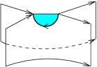
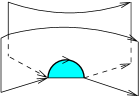
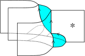
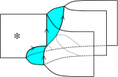
Figure 4. Some elementary foams

Intersecting such a foam with a plane results in a web, as long as the plane avoids the singularities where six facets meet, such as on the right in Figure 4.

We adapt the definition of a world-sheet foam given in [11] to our setting.

Definition 4.1.

Let $\operatorname{s_{\gamma}}$ be a finite closed oriented $4$-valent graph, which may contain disjoint circles. We assume that all edges of $\operatorname{s_{\gamma}}$ are oriented. A cycle in $\operatorname{s_{\gamma}}$ is defined to be a circle or a closed sequence of edges which form a piece-wise linear circle. Let $\Sigma$ be a compact orientable possibly disconnected surface, whose connected components are white, coloured or marked, also denoted by simple, double or triple. Each component can have a boundary consisting of several disjoint circles and can have additional decorations which we discuss below. A closed pre-foam $u$ is the identification space $\Sigma/\operatorname{s_{\gamma}}$ obtained by glueing boundary circles of $\Sigma$ to cycles in $\operatorname{s_{\gamma}}$ such that every edge and circle in $\operatorname{s_{\gamma}}$ is glued to exactly three boundary circles of $\Sigma$ and such that for any point $p\in\operatorname{s_{\gamma}}$:

1. if $p$ is an interior point of an edge, then $p$ has a neighborhood homeomorphic to the letter Y times an interval with exactly one of the facets being double, and at most one of them being triple. For an example see Figure 4;

2. if $p$ is a vertex of $\operatorname{s_{\gamma}}$, then it has a neighborhood as shown in Figure 4.

We call $\operatorname{s_{\gamma}}$ the singular graph, its edges and vertices singular arcs and singular vertices, and the connected components of $u-\operatorname{s_{\gamma}}$ the facets.

Furthermore the facets can be decorated with dots. A simple facet can only have black dots (), a double facet can also have white dots (), and a triple facet besides black and white dots can have double dots (). Dots can move freely on a facet but are not allowed to cross singular arcs. See Figure 5 for examples of pre-foams.

Figure 5. a) A pre-foam b) An open pre-foam

Note that the cycles to which the boundaries of the simple and the triple facets are glued are always oriented, whereas the ones to which the boundaries of the double facets are glued are not. Note also that there are two types of singular vertices. Given a singular vertex $v$, there are precisely two singular edges which meet at $v$ and bound a triple facet: one oriented toward $v$, denoted $e_{1}$, and one oriented away from $v$, denoted $e_{2}$. If we use the “left hand rule”, then the cyclic ordering of the facets incident to $e_{1}$ and $e_{2}$ is either $(3,2,1)$ and $(3,1,2)$ respectively, or the other way around. We say that $v$ is of type I in the first case and of type II in the second case. When we go around a triple facet we see that there have to be as many singular vertices of type I as there are of type II for the cyclic orderings of the facets to match up. This shows that for a closed pre-foam the number of singular vertices of type I is equal to the number of singular vertices of type II.

We can intersect a pre-foam $u$ generically by a plane $W$ in order to get a web, as long as the plane avoids the vertices of $\operatorname{s_{\gamma}}$. The orientation of $\operatorname{s_{\gamma}}$ determines the orientation of the simple edges of the web according to the convention in Figure 6.

Figure 6. Orientations near a singular arc

Suppose that for all but a finite number of values $i\in]0,1[$, the plane $W\times{i}$ intersects $u$ generically. Suppose also that $W\times 0$ and $W\times 1$ intersect $u$ generically and outside the vertices of $\operatorname{s_{\gamma}}$. We call $W\times I\cap u$ an open pre-foam. Interpreted as morphisms we read open pre-foams from bottom to top, and their composition consists of placing one pre-foam on top of the other, as long as their boundaries are isotopic and the orientations of the simple edges coincide.

Definition 4.2.

Let $\mathbf{Pre-foam}$ be the category whose objects are closed webs and whose morphisms are $\mathbb{Q}$-linear combinations of isotopy classes of pre-foams with the obvious identity pre-foams and composition rule.

We now define the $q$-degree of a pre-foam. Let $u$ be a pre-foam, $u_{1}$, $u_{2}$ and $u_{3}$ the disjoint union of its simple and double and marked facets respectively and $\operatorname{s_{\gamma}}(u)$ its singular graph. Define the partial $q$-gradings of $u$ as

$$q_{i}(u) = \chi(u_{i})-\frac{1}{2}\chi(\partial u_{i}\cap\partial u),\qquad i=1,2,3$$

$$q_{\operatorname{s_{\gamma}}}(u) = \chi(\operatorname{s_{\gamma}}(u))-\frac{1}{2}\chi(\partial\operatorname{s_{\gamma}}(u)).$$

where $\chi$ is the Euler characteristic and $\partial$ denotes the boundary.

Definition 4.3.

Let $u$ be a pre-foam with $d$ dots of type , $d$ dots of type and $d$ dots of type . The $q$-grading of $u$ is given by

(7) $$q(u)=-\sum_{i=1}^{3}i(N-i)q_{i}(u)-2(N-2)q_{\operatorname{s_{\gamma}}}(u)+2d+4d+6d.$$

The following result is a direct consequence of the definitions.

Lemma 4.4.

$q(u)$ is additive under the glueing of pre-foams.

5. The Kapustin-Li formula and the evaluation of closed pre-foams

Let us briefly recall the philosophy behind the pre-foams. Losely speaking, to each closed pre-foam should correspond an element in the cohomology ring of a configuration space of planes in some big $\mathbb{C}^{M}$. The singular graph imposes certain conditions on those planes. The evaluation of a pre-foam should correspond to the evaluation of the corresponding element in the cohomology ring. Of course one would need to find a consistent way of choosing the volume forms on all of those configuration spaces for this to work. However, one encounters a difficult technical problem when working out the details of this philosophy. Without explaining all the details, we can say that the problem can only be solved by figuring out what to associate to the singular vertices. Ideally we would like to find a combinatorial solution to this problem, but so far it has eluded us. That is the reason why we are forced to use the Kapustin-Li formula.

We denote a simple facet with $i$ dots by

$$\raisebox{-8.0pt}{\includegraphics[height=21.68121pt]{plan-i.eps}}.$$

Recall that $\pi_{k,m}$ can be expressed in terms of $\pi_{1,0}$ and $\pi_{1,1}$. In the philosophy explained above, the latter should correspond to and on a double facet respectively. We can then define

as being the linear combination of dotted double facets corresponding to the expression of $\pi_{k,m}$ in terms of $\pi_{1,0}$ and $\pi_{1,1}$. Analogously we expressed $\pi_{p,q,r}$ in terms of $\pi_{1,0,0}$, $\pi_{1,1,0}$ and $\pi_{1,1,1}$ (see section 3). The latter correspond to , and on a triple facet respectively, so we can make sense of

$$\raisebox{-8.0pt}{\includegraphics[height=21.68121pt]{plan-pqr.eps}}.$$

Our dot conventions and the results in proposition 6.2 will allow us to use decorated facets in exactly the same way as we did Schur polynomials in the cohomology rings of partial flag varieties.

In the sequel, we shall give a working definition of the Kapustin-Li formula for the evaluation of pre-foams and state some of its basic properties. The Kapustin-Li formula was introduced by A. Kapustin and Y. Li [5] in the context of the evaluation of 2-dimensional TQFTs and extended to the case of pre-foams by M. Khovanov and L. Rozansky in [7].

5.1. The general framework

Let $u=\Sigma/s_{\gamma}$ be a closed pre-foam with singular graph $s_{\gamma}$ and without any dots on it. Let $F$ denote an arbitrary $i$-facet, $i\in\{1,2,3\}$, with a $1$-facet being a simple facet, a $2$-facet being a double facet and a $3$-facet being a triple facet.

Recall that to each $i$-facet we associated the rational cohomology ring of the Grassmanian $\mathcal{G}_{i,N}$, i.e. $H^{*}(\mathcal{G}_{i,N},\mathbb{Q})$. Alternatively, we can associate to every $i$-facet $F$, $i$ variables $x^{F}_{1}\ldots,x^{F}_{i}$, with $\mathop{\rm deg}x^{F}_{i}=2i$, and the potential $W(x^{F}_{1},\ldots,x^{F}_{i})$, which is the polynomial defined such that

$$W(\sigma_{1},\ldots,\sigma_{i})=y_{1}^{N+1}+\ldots+y_{i}^{N+1},$$

where $\sigma_{j}$ is the $j$-th elementary symmetric polynomial in the variables $y_{1},\ldots,y_{i}$. The Jacobi algebra $J_{W}$, which is given by

$$J_{W}=\mathbb{Q}[x^{F}_{1},\ldots,x^{F}_{i}]/\langle\mathbf{\partial}W\rangle$$

where we mod out by the ideal generated by the partial derivatives of $W$, is isomorphic to $H^{*}(\mathcal{G}_{i,N},\mathbb{Q})$. Note that the top degree nonvanishing element in this Jacobi algebra is $\pi_{N-i,\ldots,N-i}$ (multiindex of length $i$), i.e. the polynomial in variables $x^{F}_{1},\ldots,x^{F}_{i}$ which gives $\pi_{N-i,\ldots,N-i}$ after replacing the variable $x^{F}_{j}$ by $\pi_{1,\ldots,1,0,\ldots,0}$ with exactly $j$ $1$’s, $1\leq j\leq i$ (see also subsection 3.1). We define the trace (volume) form, $\epsilon$, on the cohomology ring of the Grassmanian, by giving it on the basis of the Schur polynomials:

$$\epsilon(\pi_{j_{1},\ldots,j_{i}})=\begin{cases}(-1)^{\lfloor\frac{i}{2}\rfloor}&\text{if}\quad(j_{1},\ldots,j_{i})=(N-i,\ldots,N-i)\\ 0&\text{else}\end{cases}.$$

The Kapustin-Li formula associates to $u$ an element in the product of the cohomology rings of the Grassmanians (or Jacobi algebras), $J$, over all the facets in the pre-foam. Alternatively, we can see this element as a polynomial, $KL_{u}\in J$, in all the variables associated to the facets. Now, let us put some dots on $u$. Recall that a dot corresponds to an elementary symmetric polynomial. So a linear combination of dots on $u$ is equivalent to a polynomial, $f$, in the variables of the dotted facets. The value of this dotted pre-foam we define to be

(8) $$\langle u\rangle_{KL}:=\epsilon\left(\prod_{F}\dfrac{\det(\partial_{i}\partial_{j}W_{F})^{g(F)}}{(N+1)^{g^{\prime}(F)}}KL_{u}\,f\right).$$

The product is over all facets $F$ and $W_{F}$ is the potential associated to $F$. For any $i$-facet $F$, $i=1,2,3$, the symbol $g(F)$ denotes the genus of $F$ and $g^{\prime}(F)=ig(F)$.

Having explained the general idea, we are left with defining the element $KL_{u}$ for a dotless pre-foam. For that we have to explain Khovanov and Rozansky’s extension of the Kapustin-Li formula to pre-foams [7], which uses the theory of matrix factorizations.

5.2. Matrix factorizations

Let $R=\mathbb{Q}[x_{1},\ldots,x_{k}]$ be a polynomial ring, and $W\in R$. By a matrix factorization over ring $R$ with the potential $W$ we mean a triple $(M,D,W)$, where $M=M^{0}\oplus M^{1}$ ($\mathop{\rm rank}M^{0}=\mathop{\rm rank}M^{1}$) is a finite-dimensional $\mathbb{Z}/2\mathbb{Z}$-graded free $R$-module, while the (twisted) differential $D\in\mathop{\rm End}(M)$ is such that $\mathop{\rm deg}D=1$ and

(9) $$D^{2}=W\mathop{\rm Id}.$$

In other words, a matrix factorization is given by the following square matrix with polynomial entries

$$D=\left[\begin{matrix}0&D_{0}\\ D_{1}&0\end{matrix}\right],$$

such that $D_{0}D_{1}=D_{1}D_{0}=W\mathop{\rm Id}$. Matrix factorizations are also represented in the following form:

$$M^{0}{\xrightarrow{\ \ D_{0}\ \ }}M^{1}{\xrightarrow{\ \ D_{1}\ \ }}M^{0}.$$

The tensor product of two matrix factorizations with potentials $W_{1}$ and $W_{2}$ is a matrix factorization with potential $W_{1}+W_{2}$.

The dual of the matrix factorization $(M,D,W)$ is given by

$$(M,D,W)^{*}=(M^{*},D^{*},-W),$$

where

$$D^{*}=\left[\begin{matrix}0&D_{1}^{*}\\ -D_{0}^{*}&0\end{matrix}\right]$$

and $D_{i}^{*}$, $i=0,1$, is the dual map (transpose matrix) of $D_{i}$.

Throughout the paper we shall use a particular type of matrix factorizations - namely the tensor products of Koszul factorizations. For two elements $a,b\in R$, the Koszul factorization $\{a,b\}$ is defined as the matrix factorization

$$R{\xrightarrow{\ \ a\ \ }}R{\xrightarrow{\ \ b\ \ }}R.$$

Moreover if $a=(a_{1},\ldots,a_{m})\in R^{m}$ and $b=(b_{1},\ldots,b_{m})\in R^{m}$, then the tensor product of the Koszul factorization $\{a_{i},b_{i}\}$, $i=1,\ldots,m$, is denoted by

(10) $$\left(\begin{array}[]{cc}a_{1}&b_{1}\\ a_{2}&b_{2}\\ \vdots&\vdots\\ a_{m}&b_{m}\end{array}\right):=\bigotimes_{i=1}^{m}\{a_{i},b_{i}\}.$$

Sometimes we also write $\{a,b\}=\otimes_{i=1}^{m}\{a_{i},b_{i}\}$. If $\sum_{i=1}^{m}a_{i}b_{i}=0$ then $\{a,b\}$ is a 2-periodic complex, and its homology is an $R/\langle a_{1},\ldots,a_{m},b_{1},\ldots,b_{m}\rangle$-module.

5.3. Decoration of pre-foams

As we said, to each facet we associate certain variables (depending on the type of facet), a potential and the corresponding Jacobi algebra. If the variables associated to a facet $F$ are $x_{1},\ldots,x_{i}$, then we define $R_{F}=\mathbb{Q}[x_{1},\ldots,x_{i}]$.

Now we pass to the edges. To each edge, we associate a matrix factorization whose potential is equal to the signed sum of the potentials of the facets that are glued along this edge. We define it to be a certain tensor product of Koszul factorizations. In the cases we are interested in, there are always three facets glued along an edge, with two possibilities: either two simple facets and one double facet, or one simple, one double and one triple facet.

In the first case, we denote the variables of the two simple facets by $x$ and $y$ and the potentials by $x^{N+1}$ and $y^{N+1}$ respectively. To the double facet we associate the variables $s$ and $t$ and the potential $W(s,t)$. To the edge we associate the matrix factorization which is the tensor product of Koszul factorizations given by

(11) $$MF_{1}=\left(\begin{array}[]{cc}x+y-s&A^{\prime}\\ xy-t&B^{\prime}\end{array}\right),$$

where $A^{\prime}$ and $B^{\prime}$ are given by

$$A^{\prime} = \frac{W(x+y,xy)-W(s,xy)}{x+y-s},$$

$$B^{\prime} = \frac{W(s,xy)-W(s,t)}{xy-t}.$$

Note that $(x+y-s)A^{\prime}+(xy-t)B^{\prime}=x^{N+1}+y^{N+1}-W(s,t)$.

In the second case, the variable of the simple facet is $x$ and the potential is $x^{N+1}$, the variables of the double facet are $s$ and $t$ and the potential is $W(s,t)$, and the variables of the triple face are $p$, $q$ and $r$ and the potential is $W(p,q,r)$. Define the polynomials

(12) $$A = \frac{W(x+s,xs+t,xt)-W(p,xs+t,xt)}{x+s-p},$$

(13) $$B = \frac{W(p,xs+t,xt)-W(p,q,xt)}{xs+t-q},$$

(14) $$C = \frac{W(p,q,xt)-W(p,q,r)}{xt-r},$$

so that

$$(x+s-p)A+(xs+t-q)B+(xt-r)C=x^{N+1}+W(s,t)-W(p,q,r).$$

To such an edge we associate the matrix factorization given by the following tensor product of Koszul factorizations:

(15) $$MF_{2}=\left(\begin{array}[]{cc}x+s-p&A\\ xs+t-q&B\\ xt-r&C\end{array}\right).$$

In both cases, to an edge with the opposite orientation we associate the dual matrix factorization.

Next we explain what we associate to a singular vertex. First of all, for each vertex $v$, we define its local graph $\gamma_{v}$ to be the intersection of a small sphere centered at $v$ with the pre-foam. Then the vertices of $\gamma_{v}$ correspond to the edges of $u$ that are incident to $v$, to which we had associated matrix factorizations.

In this paper all local graphs are in fact tetrahedrons. However, recall that there are two types of vertices (see the remarks below definition 4.1). Label the six facets that are incident to a vertex $v$ by the numbers $1,2,3,4,5$ and $6$. Furthermore, denote the edge along which are glued the facets $i$, $j$ and $k$ by $(ijk)$. Denote the matrix factorization associated to the edge $(ijk)$ by $M_{ijk}$, if the edge points toward $v$, and by $M_{ijk}^{*}$, if the edge points away from $v$. Note that $M_{ijk}$ and $M_{ijk}^{*}$ are both defined over $R_{i}\otimes R_{j}\otimes R_{k}$.

Now we can take the tensor product of these four matrix factorizations, over the polynomial rings of the facets of the pre-foam, that correspond to the vertices of $\gamma_{v}$. This way we obtain the matrix factorization $M_{v}$, whose potential is equal to $0$, and so it is a 2-periodic chain complex and we can take its homology. To each vertex $v$ we associate an element $O_{v}\in H^{*}(M_{v})$.

More precisely, if $v$ is of type I, then

(16) $$\begin{array}[]{rcl}H^{*}(M_{v})&\cong&\mathop{\rm Ext}\left(MF_{1}(x,y,s_{1},t_{1})\otimes_{s_{1},t_{1}}MF_{2}(z,s_{1},t_{1},p,q,r)\right.,\\ &&\left.MF_{1}(y,z,s_{2},t_{2})\otimes_{s_{2},t_{2}}MF_{2}(x,s_{2},t_{2},p,q,r)\right).\end{array}$$

If $v$ is of type II, then

(17) $$\begin{array}[]{rcl}H^{*}(M_{v})&\cong&\mathop{\rm Ext}\left(MF_{1}(y,z,s_{2},t_{2})\otimes_{s_{2},t_{2}}MF_{2}(x,s_{2},t_{2},p,q,r)\right.,\\ &&\left.MF_{1}(x,y,s_{1},t_{1})\otimes_{s_{1},t_{1}}MF_{2}(z,s_{1},t_{1},p,q,r)\right).\end{array}$$

Both isomorphisms hold up to a global shift in $q$. Note that

$$MF_{1}(x,y,s_{1},t_{1})\otimes_{s_{1},t_{1}}MF_{2}(z,s_{1},t_{1},p,q,r)\simeq MF_{1}(y,z,s_{2},t_{2})\otimes_{s_{2},t_{2}}MF_{2}(x,s_{2},t_{2},p,q,r),$$

because both tensor products are homotopy equivalent to

$$\left(\begin{array}[]{cc}x+y+z-p&*\\ xy+xz+yz-q&*\\ xyz-r&*\end{array}\right).$$

We have not specified the r.h.s. of the latter Koszul factorizations, because by theorem 2.1 in [8] we have $\{a,b\}\simeq\{a,b^{\prime}\}$ if $\sum a_{i}b_{i}=\sum a_{i}b_{i}^{\prime}$ and if the sequence $\{a_{i}\}$ is regular. If $v$ is of type I, we take $O_{v}$ to be the cohomology class of a fixed degree $0$ homotopy equivalence

$$w_{v}\colon MF_{1}(x,y,s_{1},t_{1})\otimes_{s_{1},t_{1}}MF_{2}(z,s_{1},t_{1},p,q,r)\to MF_{1}(y,z,s_{2},t_{2})\otimes_{s_{2},t_{2}}MF_{2}(x,s_{2},t_{2},p,q,r).$$

The choice of $O_{v}$ is unique up to a scalar, because the $q$-dimension of the $\mathop{\rm Ext}$-group in (16) is equal to

$$q^{3N-6}\mathop{\rm qdim}(H^{*}(M_{v}))=q^{3N-6}[N][N-1][N-2]=1+q(\ldots),$$

where $(\ldots)$ is a polynomial in $q$. Note that $M_{v}$ is homotopy equivalent to the matrix factorization which corresponds to the closure of $\Upsilon$ in [6], which allows one to compute the $q$-dimension above using the results in the latter paper. If $v$ is of type II, we take $O_{v}$ to be the cohomology class of the homotopy inverse of $w_{v}$. Note that a particular choice of $w_{v}$ fixes $O_{v}$ for both types of vertices and that the value of the Kapustin-Li formula for a closed pre-foam does not depend on that choice because there are as many singular vertices of type I as there are of type II (see the remarks below definition 4.1). We do not know an explicit formula for $O_{v}$. Although such a formula would be very interesting to have, we do not need it for the purposes of this paper.

5.4. The Kapustin-Li derivative and the evaluation of closed pre-foams

From the definition, every boundary component of each facet $F$ is either a circle or a cyclicly ordered finite sequence of edges, such that the beginning of the next edge corresponds to the end of the previous edge. For every boundary component we choose an edge $e$ - the value of the Kapustin-Li formula does not depend on this choice. Denote the differential of the matrix factorization associated to this edge by $D_{e}$.

The associated Kapustin-Li derivative of $D_{e}$ in the variables $x_{1},\ldots,x_{k}$ associated to the facet $F$, is an element from $\mathop{\rm End}(M)\cong M\otimes M^{*}$, given by:

(18) $$O_{F,e}=\partial D_{e}\hat{\ }=\frac{1}{k!}\sum_{\sigma\in S_{k}}(\mathop{\rm sgn}{\sigma}){\partial_{\sigma(1)}D_{e}\partial_{\sigma(2)}D_{e}\ldots\partial_{\sigma(k)}D_{e}},$$

where $S_{k}$ is the set of all permutations of the set $\{1,\ldots,k\}$, and $\partial_{i}D$ is the partial derivative of $D$ with respect to the variable $x_{i}$. Note that $e$ can be the preferred edge for more than one facet. In general, let $O_{e}$ be the product of $O_{F,e}$ over all facets $F$ for which $e$ is the preferred edge. The order of the factors in this product is irrelevant, because they commute (see [7]). If $e$ is not the preferred edge for any $F$, we take $O_{e}$ to be the identity.

Finally, around each boundary component of $\partial F$, for each facet $F$, we contract all tensor factors $O_{e}$ and $O_{v}$. Note that one has to use super-contraction in order to get the right signs.

For a better understanding of the Kapustin-Li formula, consider the special case of a theta pre-foam $\Theta$. There are three facets $F_{1}$, $F_{2}$, $F_{3}$ which are glued along a common circle $c$, which is the preferred edge for all three. We associated a certain matrix factorization $M$ to $c$ with differential $D$. Let $\partial D_{1}\hat{\ }$, $\partial D_{2}\hat{\ }$ and $\partial D_{3}\hat{\ }$ be the Kapustin-Li derivatives of $D$ with respect to the variables of the facets $F_{1}$, $F_{2}$ and $F_{3}$, respectively. Then we have

(19) $$KL_{\Theta}={\mathop{\rm Tr}}^{s}({\partial}D_{1}\hat{\ }{\partial}D_{2}\hat{\ }{\partial}D_{3}\hat{\ }).$$

As a matter of fact we will see that we have to normalize the Kapustin-Li formula in order to get “nice values”.

5.5. Dot conversion and dot migration

The pictures related to the computations in this subsection and the next three can be found in Proposition 6.2.

Since $KL_{u}$ takes values in the tensor product of the Jacobian algebras of the potentials associated to the facets of $u$, we see that for a simple facet we have $x^{N}=0$, for a double facet $\pi_{i,j}=0$ if $i\geq N-1$, and for a triple facet $\pi_{p,q,r}=0$ if $p\geq N-2$. We call these the dot conversion relations.

To each edge along which two simple facets with variables $x$ and $y$ and one double facet with the variables $s$ and $t$ are glued, we associated the matrix factorization $MF_{1}$ with entries $x+y-s$ and $xy-t$. Therefore $\mathop{\rm Ext}(MF_{1},MF_{1})$ is a module over $R/\langle x+y-s,xy-t\rangle$. Hence, we obtain the dot migration relations along this edge.

Analogously, to the other type of singular edge along which are glued a simple facet with variable $x$, a double facet with variable $s$ and $t$, and a triple facet with variables $p$, $q$ and $r$, we associated the matrix factorization $MF_{2}$ and $\mathop{\rm Ext}(MF_{2},MF_{2})$ is a module over $R/\langle x+s-p,xs+t-q,xt-r\rangle$, and hence we obtain the dot migration relations along this edge.

5.6. $(1,1,2)-$Theta

Recall that $W(s,t)$ is the polynomial such that $W(x+y,xy)=x^{N+1}+y^{N+1}$. More precisely, we have

(20) $$W(s,t)=\sum_{i+2j=N+1}a_{ij}s^{i}t^{j},$$

with $a_{N+1,0}=1$, $a_{N+1-2j,j}=\frac{(-1)^{j}}{j}(N+1){N-j\choose j-1}$, for $2\leq 2j\leq N+1$, and $a_{ij}=0$ otherwise. In particular $a_{N-1,1}=-(N+1)$. Then we have

(21) $$W^{\prime}_{1}(s,t)=\sum_{i+2j=N+1}ia_{ij}s^{i-1}t^{j},$$

(22) $$W^{\prime}_{2}(s,t)=\sum_{i+2j=N+1}ja_{ij}s^{i}t^{j-1}.$$

By $W^{\prime}_{1}(s,t)$ and $W^{\prime}_{2}(s,t)$, we denote the partial derivatives of $W(s,t)$ with respect to the first and the second variable, respectively.

To the singular circle of a standard theta pre-foam with two simple facets, with variables $x$ and $y$ respectively, and one double facet, with variables $s$ and $t$, we assign the matrix factorization $MF_{1}$:

(23) $$MF_{1}=\left(\begin{array}[]{cc}x+y-s&A^{\prime}\\ xy-t&B^{\prime}\end{array}\right).$$

Recall that

(24) $$A^{\prime} = \frac{W(x+y,xy)-W(s,xy)}{x+y-s},$$

(25) $$B^{\prime} = \frac{W(s,xy)-W(s,t)}{xy-t}.$$

Hence, the differential of this matrix factorization is given by the following 4 by 4 matrix:

(26) $$D=\left[\begin{array}[]{cc}0&D_{0}\\ D_{1}&0\end{array}\right],$$

where

(27) $$D_{0}=\left[\begin{array}[]{cc}x+y-s&-B^{\prime}\\ xy-t&A^{\prime}\end{array}\right],\quad D_{1}=\left[\begin{array}[]{cc}A^{\prime}&B^{\prime}\\ t-xy&x+y-s\end{array}\right].$$

The Kapustin-Li formula assigns the polynomial, $KL_{\Theta_{1}}(x,y,s,t)$, which is given by the supertrace of the twisted differential of $D$

(28) $$KL_{\Theta_{1}}={\mathop{\rm Tr}}^{s}\left(\partial_{x}D\partial_{y}D\frac{1}{2}(\partial_{s}D\partial_{t}D-\partial_{t}D\partial_{s}D)\right).$$

Straightforward computation gives

(29) $$KL_{\Theta_{1}}=B^{\prime}_{s}(A^{\prime}_{x}-A^{\prime}_{y})+(A^{\prime}_{x}+A^{\prime}_{s})(B^{\prime}_{y}+xB^{\prime}_{t})-(A^{\prime}_{y}+A^{\prime}_{s})(B^{\prime}_{x}+yB^{\prime}_{t}),$$

where by $A^{\prime}_{i}$ and $B^{\prime}_{i}$ we have denoted the partial derivatives with respect to the variable $i$. From the definitions (24) and (25) we have

$$A^{\prime}_{x}-A^{\prime}_{y} = (y-x)\frac{W^{\prime}_{2}(x+y,xy)-W^{\prime}_{2}(s,xy)}{x+y-s},$$

$$A^{\prime}_{x}+A^{\prime}_{s} = \frac{W^{\prime}_{1}(x+y,xy)-W^{\prime}_{1}(s,xy)+y(W^{\prime}_{2}(x+y,xy)-W^{\prime}_{2}(s,xy))}{x+y-s},$$

$$A^{\prime}_{y}+A^{\prime}_{s} = \frac{W^{\prime}_{1}(x+y,xy)-W^{\prime}_{1}(s,xy)+x(W^{\prime}_{2}(x+y,xy)-W^{\prime}_{2}(s,xy))}{x+y-s},$$

$$B^{\prime}_{s} = \frac{W^{\prime}_{1}(s,xy)-W^{\prime}_{1}(s,t)}{xy-t},$$

$$B^{\prime}_{x}+yB^{\prime}_{t} = y\frac{W^{\prime}_{2}(s,xy)-W^{\prime}_{2}(s,t)}{xy-t},$$

$$B^{\prime}_{y}+xB^{\prime}_{t} = x\frac{W^{\prime}_{2}(s,xy)-W^{\prime}_{2}(s,t)}{xy-t}.$$

After substituting this back into (29), we obtain

(30) $$KL_{\Theta_{1}}=(y-x)\left|\begin{array}[]{cc}\alpha&\beta\\ \gamma&\delta\end{array}\right|,$$

where

$$\alpha = \frac{W^{\prime}_{1}(x+y,xy)-W^{\prime}_{1}(s,xy)}{x+y-s},$$

$$\beta = \frac{W^{\prime}_{2}(x+y,xy)-W^{\prime}_{2}(s,xy)}{x+y-s},$$

$$\gamma = \frac{W^{\prime}_{1}(s,xy)-W^{\prime}_{1}(s,t)}{xy-t},$$

$$\delta = \frac{W^{\prime}_{2}(s,xy)-W^{\prime}_{2}(s,t)}{xy-t}.$$

From this formula we see that $KL_{\Theta_{1}}$ is homogeneous of degree $4N-6$ (remember that $\mathop{\rm deg}x=\mathop{\rm deg}y=\mathop{\rm deg}s=2$ and $\mathop{\rm deg}\,t=4$).

Since the evaluation is in the product of the Grassmanians corresponding to the three disks, i.e. in the ring $\mathbb{Q}[x]/x^{N}\times\mathbb{Q}[y]/y^{N}\times\mathbb{Q}[s,t]/\langle W^{\prime}_{1}(s,t),W^{\prime}_{2}(s,t)\rangle$, we have $x^{N}=y^{N}=0=W^{\prime}_{1}(s,t)=W^{\prime}_{2}(s,t)$. Also, we can express the monomials in $s$ and $t$ as linear combinations of the Schur polynomials $\pi_{k,l}$ (writing $s=\pi_{1,0}$ and $t=\pi_{1,1})$), and we have $W^{\prime}_{1}(s,t)=(N+1)\pi_{N,0}$ and $W^{\prime}_{2}(s,t)=-(N+1)\pi_{N-1,0}$. Hence, we can write $KL_{\Theta_{1}}$ as

$$KL_{\Theta_{1}}=(y-x)\sum_{N-2\geq k\geq l\geq 0}{\pi_{k,l}p_{kl}(x,y)},$$

with $p_{kl}$ being a polynomial in $x$ and $y$. We want to determine which combinations of dots on the simple facets give rise to non-zero evaluations, so our aim is to compute the coefficient of $\pi_{N-2,N-2}$ in the sum on the r.h.s. of the above equation (i.e. in the determinant in (30)). For degree reasons, this coefficient is of degree zero, and so we shall only compute the parts of $\alpha$, $\beta$, $\gamma$ and $\delta$ which do not contain $x$ and $y$. We shall denote these parts by putting a bar over the Greek letters. Thus we have

$$\bar{\alpha} = (N+1)s^{N-1},$$

$$\bar{\beta} = -(N+1)s^{N-2},$$

$$\bar{\gamma} = \sum_{i+2j=N+1,\,j\geq 1}ia_{ij}s^{i-1}t^{j-1},$$

$$\bar{\delta} = \sum_{i+2j=N+1,\,j\geq 2}ja_{ij}s^{i}t^{j-2}.$$

Note that we have

$$t\bar{\gamma}+(N+1)s^{N}=W^{\prime}_{1}(s,t),$$

and

$$t\bar{\delta}-(N+1)s^{N-1}=W^{\prime}_{2}(s,t),$$

and so in the cohomology ring of the Grassmanian $\mathcal{G}_{2,N}$, we have $t\bar{\gamma}=-(N+1)s^{N}$ and $t\bar{\delta}=(N+1)s^{N-1}$. On the other hand, by using $s=\pi_{1,0}$ and $t=\pi_{1,1}$, we obtain that in $H^{*}(\mathcal{G}_{2,N})\cong\mathbb{Q}[s,t]/\langle\pi_{N-1,0},\pi_{N,0}\rangle$, the following holds:

$$s^{N-2}=\pi_{N-2,0}+tq(s,t),$$

for some polynomial $q$, and so

$$s^{N-1}=s^{N-2}s=\pi_{N-1,0}+\pi_{N-2,1}+stq(s,t)=t(\pi_{N-3,0}+sq(s,t)).$$

Thus, we have

$$\left|\begin{array}[]{cc}\bar{\alpha}&\bar{\beta}\\ \bar{\gamma}&\bar{\delta}\end{array}\right| = (N+1)(\pi_{N-3,0}+sq(s,t))t\bar{\delta}+(N+1)\pi_{N-2,0}\bar{\gamma}+(N+1)q(s,t)t\bar{\gamma}$$

$$= (N+1)^{2}(\pi_{N-3,0}+sq(s,t))s^{N-1}+(N+1)\pi_{N-2,0}\bar{\gamma}-(N+1)^{2}q(s,t)s^{N}$$

(34) $$= (N+1)^{2}\pi_{N-3,0}s^{N-1}+(N+1)\pi_{N-2,0}\bar{\gamma}.$$

Since

$$\bar{\gamma}=(N-1)a_{N-1,1}s^{N-2}+tr(s,t)$$

holds in the cohomology ring of Grassmanian, for some polynomial $r(s,t)$, we have

$$\pi_{N-2,0}\bar{\gamma}=\pi_{N-2,0}(N-1)a_{N-1,1}s^{N-2}=-\pi_{N-2,0}(N-1)(N+1)s^{N-2}.$$

Also, we have that for every $k\geq 2$,

$$s^{k}=\pi_{k,0}+(k-1)\pi_{k-1,1}+t^{2}w(s,t),$$

for some polynomial $w$. Replacing this in (34) and bearing in mind that $\pi_{i,j}=0$, for $i\geq N-1$, we get

$$\left|\begin{array}[]{cc}\bar{\alpha}&\bar{\beta}\\ \bar{\gamma}&\bar{\delta}\end{array}\right| = (N+1)^{2}s^{N-2}(\pi_{N-2,0}+\pi_{N-3,1}-(N-1)\pi_{N-2,0})$$

$$= (N+1)^{2}(\pi_{N-2,0}+(N-3)\pi_{N-3,1}+\pi_{2,2}w(s,t))(\pi_{N-3,1}-(N-2)\pi_{N-2,0})$$

(38) $$= -(N+1)^{2}\pi_{N-2,N-2}.$$

Hence, we have

$$KL_{\Theta_{1}}=(N+1)^{2}(x-y)\pi_{N-2,N-2}+\sum_{N-2\geq k\geq l\geq 0\atop N-2>l}c_{i,j,k,l}\pi_{k,l}x^{i}y^{j}.$$

Recall that in the product of the Grassmanians corresponding to the three disks, i.e. in the ring $\mathbb{Q}[x]/x^{N}\times\mathbb{Q}[y]/y^{N}\times\mathbb{Q}[s,t]/\langle\pi_{N-1,0},\pi_{N,0}\rangle$, we have

$$\epsilon(x^{N-1}y^{N-1}\pi_{N-2,N-2})=-1.$$

Therefore the only monomials $f$ in $x$ and $y$ such that $\langle KL_{\Theta_{1}}f\rangle_{KL}\neq 0$ are $f_{1}=x^{N-2}y^{N-1}$ and $f_{2}=x^{N-1}y^{N-2}$, and $\langle KL_{\Theta_{1}}f_{1}\rangle_{KL}=-(N+1)^{2}$ and $\langle KL_{\Theta_{1}}f_{2}\rangle=(N+1)^{2}$. Thus, we have that the value of the theta pre-foam with unlabelled 2-facet is nonzero only when the first 1-facet has $N-2$ dots and the second one has $N-1$ dots (and has the value $-(N+1)^{2}$) and when the first 1-facet has $N-1$ dots and the second one has $N-2$ dots (and has the value $(N+1)^{2}$). The evaluation of this theta foam with other labellings can be obtained from the result above by dot migration.

5.7. $(1,2,3)-$Theta

For this theta the method is the same as in the previous case, just the computations are more complicated. In this case, we have one 1-facet, to which we associate the variable $x$, one 2-facet, with variables $s$ and $t$ and the 3-facet with variables $p$, $q$ and $r$. Recall that the polynomial $W(p,q,r)$ is such that $W(a+b+c,ab+bc+ac,abc)=a^{N+1}+b^{N+1}+c^{N+1}$. We denote by $W^{\prime}_{i}(p,q,r)$, $i=1,2,3$, the partial derivative of $W$ with respect to $i$-th variable. Also, let $A$, $B$ and $C$ be the polynomials such that

(39) $$A = \frac{W(x+s,xs+t,xt)-W(p,xs+t,xt)}{x+s-p},$$

(40) $$B = \frac{W(p,xs+t,xt)-W(p,q,xt)}{xs+t-q},$$

(41) $$C = \frac{W(p,q,xt)-W(p,q,r)}{xt-r}.$$

To the singular circle of this theta pre-foam, we associated the matrix factorization (see (12)-(15)):

$$MF_{2}=\left(\begin{array}[]{cc}x+s-p&A\\ xs+t-q&B\\ xt-r&C\end{array}\right).$$

The differential of this matrix factorization is the 8 by 8 matrix

(42) $$D=\left[\begin{array}[]{cc}0&D_{0}\\ D_{1}&0\end{array}\right],$$

where

(43) $$D_{0}=\left[\begin{array}[]{c|c}d_{0}&-C\,I_{2}\\ \hline\cr(xt-r)I_{2}&d_{1}\end{array}\right],$$

(44) $$D_{1}=\left[\begin{array}[]{c|c}d_{1}&C\,I_{2}\\ \hline\cr(r-xt)I_{2}&d_{0}\\ \end{array}\right].$$

Here $d_{0}$ and $d_{1}$ are the differentials of the matrix factorization

$$\left(\begin{array}[]{cc}x+s-p&A\\ xs+t-q&B\end{array}\right),$$

i.e.

$$d_{0}=\left[\begin{array}[]{cc}x+s-p&-B\\ xs+t-q&A\end{array}\right],\quad\quad d_{1}=\left[\begin{array}[]{cc}A&B\\ q-xs-t&x+s-p\end{array}\right].$$

The Kapustin-Li formula assigns to this theta pre-foam the polynomial $KL_{\Theta_{2}}(x,s,t,p,q,r)$ given as the supertrace of the twisted differential of $D$, i.e.

$$KL_{\Theta_{2}}={\mathop{\rm Tr}}^{s}\left(\partial_{x}D\frac{1}{2}(\partial_{s}D\partial_{t}D-\partial_{t}D\partial_{s}D)\partial_{3}D\hat{\ }\right),$$

where

$$\partial_{3}D\hat{\ } = \frac{1}{3!}\left(\partial_{p}D\partial_{q}D\partial_{r}D-\partial_{p}D\partial_{r}D\partial_{q}D+\partial_{q}D\partial_{r}D\partial_{p}D-\right.$$

$$\left.\partial_{q}D\partial_{p}D\partial_{r}D+\partial_{r}D\partial_{p}D\partial_{q}D-\partial_{r}D\partial_{q}D\partial_{p}D\right).$$

After straightforward computations and some grouping, we obtain

$$KL_{\Theta_{2}} = -(A_{p}+A_{s})[(B_{t}+B_{q})(C_{x}+tC_{r})-(B_{x}+sB_{q})(C_{t}+xC_{r})-(B_{x}-sB_{t})C_{q}]$$

$$-\ (A_{p}+A_{x})[(B_{s}+xB_{q})(C_{t}+xC_{r})+(B_{s}-xB_{t})C_{q}]$$

$$-\ (A_{x}-A_{s})[B_{p}(C_{t}+xC_{r})-(B_{t}+B_{q})C_{p}+B_{p}C_{q}]$$

$$+\ A_{t}[((B_{s}+xB_{q})+B_{p})(C_{x}+tC_{r})+((B_{s}+xB_{q})$$

$$+\ (B_{x}+sB_{q}))C_{p}+((sB_{s}-xB_{x})+(s-x)B_{p})C_{q}].$$

In order to simplify this expression, we introduce the following polynomials

$$a_{1i} = \frac{W^{\prime}_{i}(x+s,xs+t,xt)-W^{\prime}_{i}(p,xs+t,xt)}{x+s-p},\quad i=1,2,3,$$

$$a_{2i} = \frac{W^{\prime}_{i}(p,xs+t,xt)-W^{\prime}_{i}(p,q,xt)}{xs+t-q},\qquad\qquad i=1,2,3,$$

$$a_{3i} = \frac{W^{\prime}_{i}(p,q,xt)-W^{\prime}_{i}(p,q,r)}{xt-r},\qquad\qquad\qquad i=1,2,3.$$

Then from (39)-(41), we have

$$A_{x}+A_{p}=a_{11}+sa_{12}+ta_{13},\quad A_{p}+A_{s}=a_{11}+xa_{12},$$

$$A_{x}-A_{s}=(s-x)a_{12}+ta_{13},\quad A_{t}=a_{12}+xa_{13},$$

$$B_{p}=a_{21},\quad B_{s}-xB_{t}=-x^{2}a_{23},$$

$$sB_{s}-xB_{x}=xta_{23},\quad B_{x}-sB_{t}=(t-sx)a_{23},$$

$$B_{t}+B_{q}=a_{22}+xa_{23},\quad B_{x}+sB_{q}=sa_{22}+ta_{23},B_{s}+xB_{q}=xa_{22},$$

$$C_{p}=a_{31},\quad C_{q}=a_{32},\quad C_{x}+tC_{r}=ta_{33},\quad C_{t}+xC_{r}=xa_{33}.$$

Using this $KL_{\Theta_{2}}$ becomes

$$KL_{\Theta_{2}}=-(t-sx+x^{2})\left|\begin{array}[]{ccc}a_{11}&a_{12}&a_{13}\\ a_{21}&a_{22}&a_{23}\\ a_{31}&a_{32}&a_{33}\end{array}\right|.$$

Now the last part follows analogously as in the case of the $(1,1,2)$-theta pre-foam. For degree reasons the coefficient of $\pi_{N-3,N-3,N-3}$ in the latter determinant is of degree zero, and one can obtain that it is equal to $(N+1)^{3}$. Thus, the coefficient of $\pi_{N-3,N-3,N-3}$ in $KL_{\Theta_{2}}$ is $-(N+1)^{3}(t-sx+x^{2})$ from which we obtain the value of the theta pre-foam when the 3-facet is undotted. For example, we see that

$$\epsilon(KL_{\Theta_{2}}\pi_{1,1}(s,t)^{N-3}x^{N-1})=-(N+1)^{3}.$$

It is then easy to obtain the values when the 3-facet is labelled by $\pi_{N-3,N-3,N-3}(p,q,r)$ using dot migration. The example above implies that

$$\epsilon(KL_{\Theta_{2}}\pi_{N-3,N-3,N-3}(p,q,r)x^{2})=-(N+1)^{3}.$$

5.8. Spheres

The values of dotted spheres are easy to compute. Note that for any sphere with dots $f$ the Kapustin-Li formula gives

$$\epsilon(f).$$

Therefore for a simple sphere we get $1$ if $f=x^{N-1}$, for a double sphere we get $-1$ if $f=\pi_{N-2,N-2}$ and for a triple sphere we get $-1$ if $f=\pi_{N-3,N-3,N-3}$.

5.9. Normalization

It will be convenient to normalize the Kapustin-Li evaluation. Let $u$ be a closed pre-foam with graph $\Gamma$. Note that $\Gamma$ has two types of edges: the ones incident to two simple facets and one double facet and the ones incident to one simple, one double and one triple facet. Edges of the same type form cycles in $\Gamma$. Let $e_{112}(u)$ be the total number of cycles in $\Gamma$ with edges of the first type and $e_{123}(u)$ the total number of cycles with edges of the second type. We normalize the Kapustin-Li formula by dividing $KL_{u}$ by

$$(N+1)^{2e_{112}+3e_{123}}.$$

In the sequel we only use this normalized Kapustin-Li evaluation keeping the same notation $\langle u\rangle_{KL}$. Note that the numbers $e_{112}(u)$ and $e_{123}(u)$ are invariant under the relation (MP). Note also that with this normalization the KL-evaluation in the examples above always gives $0,-1$ or $1$.

5.10. The glueing property

If $u$ is an open pre-foam whose boundary consists of two parts $\Gamma_{1}$ and $\Gamma_{2}$, then the Kapustin-Li formula associates to $u$ an element from $\mathop{\rm Ext}(M_{1},M_{2})$, where $M_{1}$ and $M_{2}$ are matrix factorizations associated to $\Gamma_{1}$ and $\Gamma_{2}$ respectively. If $u^{\prime}$ is another pre-foam whose boundary consists of $\Gamma_{2}$ and $\Gamma_{3}$, then it corresponds to an element from $\mathop{\rm Ext}(M_{2},M_{3})$, while the element associated to the pre-foam $uu^{\prime}$, which is obtained by gluing the pre-foams $u$ and $u^{\prime}$ along $\Gamma_{2}$, is equal to the composite of the elements associated to $u$ and $u^{\prime}$.

On the other hand, we can see $u$ as a morphism from the empty set to its boundary $\Gamma=\Gamma_{2}\cup\overline{\Gamma_{1}}$, where $\overline{\Gamma_{1}}$ is equal to $\Gamma_{1}$ but with the opposite orientation. In that case, the Kapustin-Li formula associates to it an element from

$$\mathop{\rm Ext}(\emptyset,M_{\Gamma_{2}}\otimes M_{\Gamma_{1}}^{*})\cong H^{*}(\Gamma).$$

Of course both ways of applying the Kapustin-Li formula are equivalent up to a global $q$-shift by corollary 6 in [6].

In the case of a pre-foam $u$ with corners, i.e. a pre-foam with two horizontal boundary components $\Gamma_{1}$ and $\Gamma_{2}$ which are connected by vertical edges, one has to “pinch” the vertical edges. This way one can consider $u$ to be a morphism from the empty set to $\Gamma_{2}\cup_{v}\overline{\Gamma_{1}}$, where $\cup_{v}$ means that the webs are glued at their vertices. The same observations as above hold, except that $M_{\Gamma_{2}}\otimes M_{\Gamma_{1}}^{*}$ is now the tensor product over the polynomial ring in the variables associated to the horizontal edges with corners.

6. The category $\mathbf{Foam}_{N}$

Recall that $\langle u\rangle_{KL}$ denotes the Kapustin-Li evaluation of a closed pre-foam $u$.

Definition 6.1.

The category $\mathbf{Foam}_{N}$ is the quotient of the category $\mathbf{Pre-foam}$ by the kernel of $\langle\;\rangle_{KL}$, i.e. by the following identifications: for any webs $\Gamma$, $\Gamma^{\prime}$ and finite sets $f_{i}\in\mbox{Hom}_{\mathbf{Pre-foam}}\left(\Gamma,\Gamma^{\prime}\right)$ and $c_{i}\in\mathbb{Q}$ we impose the relations

$$\sum\limits_{i}c_{i}f_{i}=0\quad\Leftrightarrow\quad\sum\limits_{i}c_{i}\langle g^{\prime}f_{i}g\rangle_{KL}=0,$$

for all $g\in\mbox{Hom}_{\mathbf{Pre-foam}}\left(\emptyset,\Gamma\right)$ and $g^{\prime}\in\mbox{Hom}_{\mathbf{Pre-foam}}\left(\Gamma^{\prime},\emptyset\right)$. The morphisms of $\mathbf{Foam}_{N}$ are called foams.

In the next two propositions we prove the “principal” relations in $\mathbf{Foam}_{N}$. All other relations that we need are consequences of these and will be proved in subsequent lemmas and corollaries.

Proposition 6.2.

The following identities hold in $\mathbf{Foam}_{N}$:

(The dot conversion relations)

$$\raisebox{-8.0pt}{\includegraphics[height=21.68121pt]{plan-i.eps}}=0\quad\mbox{if}\quad i\geq N.$$

$$\quad\ \ \raisebox{-8.0pt}{\includegraphics[height=21.68121pt]{dplan-km.eps}}=0\quad\mbox{if}\quad k\geq N-1.$$

$$\quad\ \ \raisebox{-8.0pt}{\includegraphics[height=21.68121pt]{plan-pqr.eps}}=0\quad\mbox{if}\quad p\geq N-2.$$

(The dot migration relations)

$$= \quad\raisebox{-12.0pt}{\includegraphics[height=28.90755pt]{pdots_1.eps}}\ +\ \raisebox{-12.0pt}{\includegraphics[height=28.90755pt]{pdots_2.eps}}$$

$$=$$

$$= \ \raisebox{-12.0pt}{\includegraphics[height=28.90755pt]{pdots-star-db.eps}}\ +\ \raisebox{-12.0pt}{\includegraphics[height=28.90755pt]{pdots_4.eps}}$$

$$= \ \raisebox{-12.0pt}{\includegraphics[height=28.90755pt]{pdotsd_w1.eps}}\ +\ \raisebox{-12.0pt}{\includegraphics[height=28.90755pt]{pdots-star-bdb.eps}}$$

$$=$$

(The cutting neck relations)

$$\raisebox{-27.0pt}{\includegraphics[height=57.81621pt]{cylinder.eps}}=\sum\limits_{i=0}^{N-1}\raisebox{-27.0pt}{\includegraphics[height=57.81621pt]{cneck-i.eps}}\quad\text{(CN${}_{1}$)}$$

$$\raisebox{-28.0pt}{\includegraphics[height=57.81621pt]{dcylinder.eps}}=-\sum\limits_{0\leq j\leq i\leq N-2}\raisebox{-28.0pt}{\includegraphics[height=57.81621pt]{dcneck-ij.eps}}\quad\text{(CN${}_{2}$)}\qquad\qquad\raisebox{-28.0pt}{\includegraphics[height=57.81621pt]{cylinder-star.eps}}=-\sum\limits_{0\leq k\leq j\leq i\leq N-3}\raisebox{-28.0pt}{\includegraphics[height=57.81621pt]{cneck-ijk.eps}}\quad\text{(CN${}_{*}$)}$$

(The sphere relations)

$$\raisebox{-10.0pt}{\includegraphics[height=25.29494pt]{sph-i.eps}}=\begin{cases}1,&i=N-1\\ 0,&\text{else}\end{cases}\quad\text{(S${}_{1}$)}\qquad\quad\raisebox{-10.0pt}{\includegraphics[height=25.29494pt]{dsph-ij.eps}}=\begin{cases}-1,&i=j=N-2\\ 0,&\text{else}\end{cases}\quad\text{(S${}_{2}$)}$$

$$\raisebox{-10.0pt}{\includegraphics[height=25.29494pt]{sph-star-ijk.eps}}=\begin{cases}-1,&i=j=k=N-3\\ 0,&\text{else}.\end{cases}\quad\text{(S${}_{*}$)}$$

(The $\Theta$-foam relations)

$$\raisebox{-10.0pt}{\includegraphics[height=25.29494pt]{theta12.eps}}=-1=-\ \raisebox{-10.0pt}{\includegraphics[height=25.29494pt]{theta21.eps}}\quad(\ThetaGraph)\qquad\ \text{and}\ \qquad\raisebox{-10.0pt}{\includegraphics[height=30.35326pt]{theta-star-32.eps}}=-1=-\ \raisebox{-16.0pt}{\includegraphics[height=30.35326pt]{theta-star-23.eps}}\quad({}_{*}).$$

Inverting the orientation of the singular circle of $({}_{*})$ inverts the sign of the corresponding foam. A theta-foam with dots on the double facet can be transformed into a theta-foam with dots only on the other two facets, using the dot migration relations.

(The Matveev-Piergalini relation)

$$\raisebox{-24.0pt}{\includegraphics[height=57.81621pt]{sh_move1.eps}}=\raisebox{-24.0pt}{\includegraphics[height=57.81621pt]{sh_move2.eps}},\quad\raisebox{-24.0pt}{\includegraphics[height=57.81621pt]{sh_move1-star.eps}}=\raisebox{-24.0pt}{\includegraphics[height=57.81621pt]{sh_move2-star.eps}}.\qquad\text{(MP)}$$

Proof.

The dot conversion and migration relations, the sphere relations, the theta foam relations have already been proved in section 5.

The cutting neck relations are special cases of formula (5.68) in [7], where $O_{j}$ and $O_{j}^{*}$ can be read off from our equations (6).

The Matveev-Piergalini (MP) relation is an immediate consequence of the choice of input for the singular vertices. Note that in this relation there are always two singular vertices of different type. The elements in the $\mathop{\rm Ext}$-groups associated to those two types of singular vertices are inverses of each other, which implies exactly the (MP) relation by the glueing properties explained in subsection 5.10. ∎

The following identities are a consequence of the dot and the theta relations.

Lemma 6.3.

$$\raisebox{-17.0pt}{\includegraphics[height=39.74872pt]{theta-pqrkli.eps}}=\begin{cases}-1&\text{if}\quad(p,q,r)=(N-3-i,N-2-k,N-2-j)\\ -1&\text{if}\quad(p,q,r)=(N-3-k,N-3-j,N-1-i)\\ 1&\text{if}\quad(p,q,r)=(N-3-k,N-2-i,N-2-j)\\ 0&\text{else}\end{cases}$$

Note that the first three cases only make sense if

$$N-2\geq j\geq k\geq i+1\geq 1$$

$$N-1\geq i\geq j+2\geq k+2\geq 2$$

$$N-2\geq j\geq i\geq k+1\geq 1$$

respectively.

Proof.

We denote the value of a theta foam by $\Theta(\pi_{p,q,r},\pi_{j,k},i)$. Since the $q$-degree of a non-decorated theta foam is equal to $-(N-1)-2(N-2)-3(N-3)=-(6N-14)$, we can have nonzero values of $\Theta(\pi_{p,q,r},\pi_{j,k},i)$ only if $p+q+r+j+k+i=3N-7$. Thus, if the 3-facet is not decorated, i.e. $p=q=r=0$, we have only four possibilities for the triple $(j,k,i)$ – namely $(N-2,N-2,N-3)$, $(N-2,N-3,N-2)$, $(N-2,N-4,N-1)$ and $(N-3,N-3,N-1)$. By Proposition 6.2 we have

$$\Theta(\pi_{0,0,0},\pi_{N-2,N-2},N-3)=-1.$$

However by dot migration, Lemma 3.1 and the fact that $\pi_{p,q,r}=0$ if $p\geq N-2$, we have

$$0=\Theta(\pi_{N-2,N-2,N-3},\pi_{0,0},0) = \Theta(\pi_{0,0,0},\pi_{N-2,N-2},N-3)+\Theta(\pi_{0,0,0},\pi_{N-2,N-3},N-2),$$

$$0=\Theta(\pi_{N-1,N-3,N-3},\pi_{0,0},0) = \Theta(\pi_{0,0,0},\pi_{N-2,N-3},N-2)+\Theta(\pi_{0,0,0},\pi_{N-3,N-3},N-1),$$

$$0=\Theta(\pi_{N-1,N-2,N-4},\pi_{0,0},0) = \Theta(\pi_{0,0,0},\pi_{N-2,N-2},N-3)+\Theta(\pi_{0,0,0},\pi_{N-2,N-3},N-2)+$$

$$+\Theta(\pi_{0,0,0},\pi_{N-2,N-4},N-1).$$

Thus, the only nonzero values of the theta foams, when the 3-facet is nondecorated are

$$\Theta(\pi_{0,0,0},\pi_{N-2,N-2},N-3)=\Theta(\pi_{0,0,0},\pi_{N-3,N-3},N-1)=-1,$$

$$\Theta(\pi_{0,0,0},\pi_{N-2,N-3},N-2)=+1.$$

Now we calculate the values of the general theta foam. Suppose first that $i\leq k$. Then we have

(45) $$\Theta(\pi_{p,q,r},\pi_{j,k},i)=\Theta(\pi_{p,q,r},\pi_{i,i}\pi_{j-i,k-i},i)=\Theta(\pi_{p+i,q+i,r+i},\pi_{j-i,k-i},0),$$

by dot migration. In order to calculate $\Theta(\pi_{x,y,z},\pi_{w,u},0)$ for $N-3\geq x\geq y\geq z\geq 0$ and $N-2\geq w\geq u\geq 0$, we use Lemma 3.1. By dot migration we have

(46) $$\Theta(\pi_{x,y,z},\pi_{w,u},0)=\sum_{(a,b,c)\sqsubset(x,y,z)}\Theta(\pi_{0,0,0},\pi_{w,u}\pi_{a,b},c).$$

Since $c\leq p\leq N-3$, a summand on the r.h.s. of (46) can be nonzero only for $c=N-3$ and $a$ and $b$ such that $\pi_{N-2,N-2}\in\pi_{w,u}\pi_{a,b}$, i.e. $a=N-2-u$ and $b=N-2-w$. Hence the value of (46) is equal to $-1$ if

(47) $$(N-2-u,N-2-w,N-3)\sqsubset(x,y,z),$$

and $0$ otherwise. Finally, (47) is equivalent to $x+y+z+w+u=3N-7$, $x\geq N-2-u\geq y$, $y\geq N-2-w\geq z$ and $x\geq N-3\geq z$, and so we must have $u>0$ and

$$x = N-3,$$

$$y = N-2-u,$$

$$z = N-2-w.$$

Going back to (46), we have that the value of theta is equal to $0$ if $l=i$, and in the case $l>i$ it is nonzero (and equal to $-1$) iff

$$p = N-3-i,$$

$$q = N-2-k,$$

$$r = N-2-j,$$

which gives the first family.

Suppose now that $k<i$. As in (45) we have

(48) $$\Theta(\pi_{p,q,r},\pi_{j,k},i)=\Theta(\pi_{p+k,q+k,r+k},\pi_{j-k,0},i-k).$$

Hence, we now concentrate on $\Theta(\pi_{x,y,z},\pi_{w,0},u)$ for $N-3\geq x\geq y\geq z\geq 0$, $N-2\geq w\geq 0$ and $N-1\geq u\geq 1$. Again, by using Lemma 3.1 we have

(49) $$\Theta(\pi_{x,y,z},\pi_{w,0},0)=\sum_{(a,b,c)\sqsubset(x,y,z)}\Theta(\pi_{0,0,0},\pi_{w,0}\pi_{a,b},u+c).$$

Since $a\leq N-3$, we cannot have $\pi_{N-2,N-2}\in\pi_{w,0}\pi_{a,b}$ and we can have $\pi_{N-2,N-3}\in\pi_{w,0}\pi_{a,b}$ iff $a=N-3$ and $b=N-2-w$. In this case we have a nonzero summand (equal to $1$) iff $c=N-2-u$. Finally $\pi_{N-3,N-3}\in\pi_{w,0}\pi_{a,b}$ iff $a=N-3$ and $b=N-3-w$. In this case we have a nonzero summand (equal to $-1$) iff $c=N-1-u$. Thus we have a summand on the r.h.s. of (49) equal to $+1$ iff

(50) $$(N-3,N-2-w,N-2-u)\sqsubset(x,y,z),$$

and a summand equal to $-1$ iff

(51) $$(N-3,N-3-w,N-1-u)\sqsubset(x,y,z).$$

Note that in both above cases we must have $x+y+z+w+u=3N-7$, $x=N-3$ and $u\geq 1$. Finally, the value of the r.h.s of (49) will be nonzero iff exactly one of (50) and (51) holds.

In order to find the value of the sum on r.h.s. of (49), we split the rest of the proof in three cases according to the relation between $w$ and $u$.

If $w\geq u$, (50) is equivalent to $y\geq N-2-w$, $z\leq N-2-w$, while (51) is equivalent to $y\geq N-3-w$, $z\leq N-3-w$ and $u\geq 2$. Now, we can see that the sum is nonzero and equal to $1$ iff $z=N-2-w$ and so $y=N-2-u$. Returning to (48), we have that the value of $\Theta(\pi_{p,q,r},\pi_{j,k},i)$ is equal to $1$ for

$$p = N-3-k,$$

$$q = N-2-i,$$

$$r = N-2-j,$$

for $N-2\geq j\geq i\geq k+1\geq 1$, which is our third family.

If $w\leq u-2$, (50) is equivalent to $y\geq N-2-w$, $z\leq N-2-u$ and $u\leq N-2$ while (51) is equivalent to $y\geq N-3-w$, $z\leq N-1-u$. Hence, in this case we have that the total sum is nonzero and equal to $-1$ iff $y=N-3-w$ and $z=N-1-u$, which by returning to (48) gives that the value of $\Theta(\pi_{p,q,r},\pi_{j,k},i)$ is equal to $-1$ for

$$p = N-3-k,$$

$$q = N-3-j,$$

$$r = N-1-i,$$

for $N-3\geq i-2\geq j\geq k\geq 0$, which is our second family.

Finally, if $u=w+1$ (50) becomes equivalent to $y\geq N-2-w$ and $z\leq N-3-w$, while (51) becomes $y\geq N-3-w$ and $z\leq N-3-w$. Thus, in order to have a nonzero sum, we must have $y=N-3-w$. But in that case, because of the fixed total sum of indices, we would have $z=N-1-u=N-2-w>N-3-w$, which contradicts (51). Hence, in this case, the total value of the theta foam is $0$. ∎

As a direct consequence of the previous theorem, we have

Corollary 6.4.

For fixed values of $j$, $k$ and $i$, if $j\neq i-1$ and $k\neq i$, there is exactly one triple $(p,q,r)$ such that the value of $\Theta(\pi_{p,q,r},\pi_{j,k},i)$ is nonzero. Also, if $j=i-1$ or $k=i$, the value of $\Theta(\pi_{p,q,r},\pi_{j,k},i)$ is equal to $0$ for every triple $(p,q,r)$. Hence, for fixed $i$, there are $n-1\choose 2$ 5-tuples $(p,q,r,j,k)$ such that $\Theta(\pi_{p,q,r},\pi_{j,k},i)$ is nonzero.

Conversely, for fixed $p$, $q$ and $r$, there always exist three different triples $(j,k,i)$ (one from each family), such that $\Theta(\pi_{p,q,r},\pi_{j,k},i)$ is nonzero.

Finally, for all $p$, $q$, $r$, $j$, $k$ and $i$, we have

$$\Theta(\pi_{p,q,r},\pi_{j,k},i)=\Theta(\hat{\pi}_{p,q,r},\hat{\pi}_{j,k},N-1-i).$$

The following relations are an immediate consequence of Lemma 6.3, Corollary 6.4 and (CN_i), $i=1,2,*$.

Corollary 6.5.

(52) $$\raisebox{-18.0pt}{\includegraphics[height=43.36243pt]{bubble-pqri.eps}}=\begin{cases}-\raisebox{-17.0pt}{\includegraphics[height=28.90755pt]{dplan-qr.eps}}&\text{if}\quad p=N-3-i\\ -\raisebox{-17.0pt}{\includegraphics[height=28.90755pt]{dplan-ppqq.eps}}&\text{if}\quad r=N-1-i\\ \raisebox{-17.0pt}{\includegraphics[height=28.90755pt]{dplan-ppr.eps}}&\text{if}\quad q=N-2-i\\ \qquad 0&\text{else}\end{cases}$$

(53) $$\raisebox{-18.0pt}{\includegraphics[height=43.36243pt]{bubble-ikm-star.eps}}=\begin{cases}-\raisebox{-15.0pt}{\includegraphics[height=28.90755pt]{plan-kmi.eps}}&\text{if}\quad N-2\geq k\geq m\geq i+1\geq 1\\ -\raisebox{-15.0pt}{\includegraphics[height=28.90755pt]{plan-ikm.eps}}&\text{if}\quad N-1\geq i\geq k+2\geq m+2\geq 2\\ \ \ \ \raisebox{-15.0pt}{\includegraphics[height=28.90755pt]{plan-kim.eps}}&\text{if}\quad N-2\geq k\geq i\geq m+1\geq 1\\ \qquad 0&\text{else}\end{cases}$$

(54) $$\raisebox{-18.0pt}{\includegraphics[height=46.25275pt]{bubble-pqrkm-star.eps}}=\begin{cases}\ \ \ -\raisebox{-13.0pt}{\includegraphics[height=25.29494pt]{plan-ppp.eps}}&\text{if}\quad q=N-2-m,\,\,r=N-2-k\\ \ \ \ -\raisebox{-13.0pt}{\includegraphics[height=25.29494pt]{plan-r.eps}}&\text{if}\quad p=N-3-m,\,\,q=N-3-k\\ \raisebox{-13.0pt}{\includegraphics[height=25.29494pt]{plan-qq.eps}}&\text{if}\quad p=N-3-m,\,\,r=N-2-k\\ \qquad 0&\text{else}\end{cases}$$

Lemma 6.6.

$$\raisebox{-17.0pt}{\includegraphics[height=39.74872pt]{theta-mijkk.eps}}=\begin{cases}-1&\mbox{if}\quad m+j=N-1=i+k+1\\ +1&\mbox{if}\quad j+k=N-1=i+m+1,\end{cases}$$

Proof.

By the dot conversion formulas, we get

$$\raisebox{-17.0pt}{\includegraphics[height=39.74872pt]{theta-mijkk.eps}}=\sum\limits_{\alpha=0}^{i-j}\raisebox{-17.0pt}{\includegraphics[height=39.74872pt]{theta-miakja.eps}}.$$

By $(\ThetaGraph)$ we have

$$\raisebox{-17.0pt}{\includegraphics[height=39.74872pt]{theta-miakja.eps}}=\begin{cases}-1&\text{if}\quad m+i-(N-1)=\alpha=N-2-(k+j)\\ +1&\text{if}\quad m+i-(N-2)=\alpha=N-1-(k+j)\\ 0&\text{else}.\end{cases}$$

We see that, in the sum above, the summands for two consecutive values of $\alpha$ will cancel unless one of them is zero and the other is not. We see that the total sum is equal to $-1$ if the first non-zero summand is at $\alpha=i-j$ and $+1$ if the last non-zero summand is at $\alpha=0$. ∎

The following bubble-identities are an immediate consequence of Lemma 6.6 and (CN₁) and (CN₂).

Corollary 6.7.

(55) $$\raisebox{-20.0pt}{\includegraphics[height=43.36243pt]{bubble-ij.eps}}=\begin{cases}\quad-\raisebox{-13.0pt}{\includegraphics[height=25.29494pt]{dplan-iij.eps}}&\text{if}\quad i>j\geq 0\\ \raisebox{-13.0pt}{\includegraphics[height=25.29494pt]{dplan-jji.eps}}&\text{if}\quad j>i\geq 0\\ \qquad 0&\text{if}\quad i=j\end{cases}$$

(56) $$\raisebox{-18.0pt}{\includegraphics[height=43.36243pt]{bubble-ikj.eps}}=\begin{cases}-\raisebox{-8.0pt}{\includegraphics[height=21.68121pt]{plan-kk.eps}}&\text{if }\ i+j=N-1\\ \\ \raisebox{-8.0pt}{\includegraphics[height=21.68121pt]{plan-j.eps}}&\text{if }\ i+k=N-2\\ \\ \quad\ 0&\text{ else }\end{cases}$$

The following identities follow easily from (CN₁), (CN₂), Lemma 6.3, Lemma 6.6 and their corollaries.

Corollary 6.8.

$$\raisebox{-22.0pt}{\includegraphics[height=43.36243pt]{3cyls1.eps}}+\sum_{a+b+c=N-2}\raisebox{-22.0pt}{\includegraphics[height=43.36243pt]{3cyls2.eps}}=\raisebox{-22.0pt}{\includegraphics[height=43.36243pt]{3cyls3.eps}}\hbox to0.0pt{\hskip 47.36096pt\text{\emph{(3C)}}\hss}$$

$$\raisebox{-8.0pt}{\includegraphics[height=21.68121pt]{remdisk.eps}}\ =\raisebox{-8.0pt}{\includegraphics[height=21.68121pt]{cupdcap-h.eps}}\ -\ \raisebox{-8.0pt}{\includegraphics[height=21.68121pt]{cupcapd-h.eps}}\hbox to0.0pt{\hskip 83.95807pt\text{(RD${}_{1}$)}\hss}$$

$$\raisebox{-8.0pt}{\includegraphics[height=21.68121pt]{remdisk2.eps}}\ =\raisebox{-8.0pt}{\includegraphics[height=21.68121pt]{cup2-dcap-h.eps}}\ -\ \raisebox{-8.0pt}{\includegraphics[height=21.68121pt]{cup1-dcapb-h.eps}}\ +\ \raisebox{-8.0pt}{\includegraphics[height=21.68121pt]{cup-dcapw-h.eps}}\hbox to0.0pt{\hskip 60.27759pt\text{(RD${}_{2}$)}\hss}$$

$$\raisebox{-8.0pt}{\includegraphics[height=21.68121pt]{fatcyl.eps}}\ =-\ \raisebox{-8.0pt}{\includegraphics[height=21.68121pt]{cupcap-h.eps}}\hbox to0.0pt{\hskip 79.65253pt\text{(FC)}\hss}$$

Note that by the results above we are able to compute $\langle u\rangle_{KL}$ combinatorially, for any closed foam $u$ whose singular graphs has no vertices, simply by using the cutting neck relations near all singular circles and evaluating the resulting spheres and theta foams. If the singular graph of $u$ has vertices, then we do not know if our relations are sufficient to evaluate $u$. We conjecture that they are sufficient, and that therefore our theory is strictly combinatorial, but we do not have a complete proof.

Proposition 6.9.

The following identities hold in $\mathbf{Foam}_{N}$:

(The digon removal relations)

$$\raisebox{-20.0pt}{\includegraphics[height=43.36243pt]{digonfid.eps}}=\raisebox{-20.0pt}{\includegraphics[height=43.36243pt]{dig_rem1.eps}}-\raisebox{-20.0pt}{\includegraphics[height=43.36243pt]{dig_rem2.eps}}\hbox to0.0pt{\hskip 68.88867pt\text{(DR${}_{1}$)}\hss}$$

$$\raisebox{-27.0pt}{\includegraphics[height=50.58878pt]{digonfid_b.eps}}=\sum_{a+b+c=N-2}\ \raisebox{-27.0pt}{\includegraphics[height=50.58878pt]{dig_rem_b.eps}}\ =\sum_{i=0}^{N-2}\ \raisebox{-27.0pt}{\includegraphics[height=50.58878pt]{dig_rem_b-i.eps}}\hbox to0.0pt{\hskip 30.1388pt\text{(DR${}_{2}$)}\hss}$$

$$\raisebox{-30.0pt}{\includegraphics[height=50.58878pt]{digonfid_b-star1.eps}}=\ -\raisebox{-30.0pt}{\includegraphics[height=50.58878pt]{dig_rem_b1-star.eps}}+\raisebox{-30.0pt}{\includegraphics[height=50.58878pt]{dig_rem_b2-star.eps}}-\raisebox{-30.0pt}{\includegraphics[height=50.58878pt]{dig_rem_b3-star.eps}}\hbox to0.0pt{\hskip 32.29156pt\text{(DR${}_{3_{1}}$)}\hss}$$

$$\raisebox{-30.0pt}{\includegraphics[height=50.58878pt]{digonfid_b-star2.eps}}=-\sum_{0\leq j\leq i\leq N-3}\ \raisebox{-30.0pt}{\includegraphics[height=50.58878pt]{dig_rem-32.eps}}\hbox to0.0pt{\hskip 55.97205pt\text{(DR${}_{3_{2}}$)}\hss}$$

$$\raisebox{-20.0pt}{\includegraphics[height=43.36243pt]{digonfid-star.eps}}=-\sum_{i=0}^{N-3}\raisebox{-20.0pt}{\includegraphics[height=43.36243pt]{dig_rem33.eps}}\hbox to0.0pt{\hskip 78.36084pt\text{(DR${}_{3_{3}}$)}\hss}$$

(The first square removal relation)

$$\raisebox{-31.0pt}{\includegraphics[height=65.04256pt]{sqface_id.eps}}=-\;\raisebox{-31.0pt}{\includegraphics[height=65.04256pt]{sq_rem2.eps}}\quad+\sum_{a+b+c+d=N-3}\ \raisebox{-31.0pt}{\includegraphics[height=65.04256pt]{sq_rem1.eps}}\hbox to0.0pt{\hskip 17.22217pt\text{(SqR${}_{1}$)}\hss}$$

Proof.

We first explain the idea of the proof. Naively one could try to consider all closures of the foams in a relation and compare their KL-evaluations. However, in practice we are not able to compute the KL-evaluations of arbitrary closed foams with singular vertices. Therefore we use a different strategy. We consider any foam in the proposition as a foam from $\emptyset$ to its boundary, rather than as a foam between one part of its boundary to another part. If $u$ is such a foam whose boundary is a closed web $\Gamma$, then by the properties explained in Section 5 the KL-formula associates to $u$ an element in $H^{*}(\Gamma)$, which is the homology of the complex associated to $\Gamma$ in [6]. By Definition 6.1 and by the glueing properties of the KL-formula, as explained in Section 5, the induced linear map from $\langle\ |_{KL}\colon\mathbf{Foam}_{N}(\emptyset,\Gamma)\to H^{*}(\Gamma)$ is injective. The KL-formula also defines an inner product on $\mathbf{Foam}_{N}(\emptyset,\Gamma)$ by

$$(u,v)\mapsto\langle u\hat{v}\rangle_{KL}.$$

By $\hat{v}$ we mean the foam in $\mathbf{Foam}_{N}(\Gamma,\emptyset)$ obtained by rotating $v$ along the axis which corresponds to the $y$-axis (i.e. the horizontal axis parallel to the computer screen) in the original picture in this proposition. By the results in [6] we know the dimension of $H^{*}(\Gamma)$. Suppose it is equal to $m$ and that we can find two sets of elements $u_{i}$ and $u_{i}^{*}$ in $\mathbf{Foam}_{N}(\emptyset,\Gamma)$, $i=1,2,\ldots,m$, such that

$$\langle u_{i}\widehat{u_{j}^{*}}\rangle_{KL}=\delta_{i,j},$$

where $\delta_{i,j}$ is the Kronecker delta. Then $\{u_{i}\}$ and $\{u_{i}^{*}\}$ are mutually dual bases of $\mathbf{Foam}_{N}(\emptyset,\Gamma)$ and $\langle\ |_{KL}$ is an isomorphism. Therefore, two elements $f,g\in\mathbf{Foam}_{N}(\emptyset,\Gamma)$ are equal if and only if

$$\langle f\widehat{u_{i}}\rangle_{KL}=\langle g\widehat{u_{i}}\rangle_{KL},$$

for all $i=1,2,\ldots,m$ (alternatively one can use the $u_{i}^{*}$ of course). In practice this only helps if the l.h.s. and the r.h.s. of these $m$ equations can be computed, e.g. if $f,g$ and the $u_{i}$ are all foams with singular graphs without vertices. Fortunately that is the case for all the relations in this proposition.

Let us now prove (DR₁) in detail. Note that the boundary of any of the foams in (DR₁), denoted $\Gamma$, is homeomorphic to the web

$$\raisebox{-17.0pt}{\includegraphics[height=36.135pt]{digons1web.eps}}.$$

Recall that the dimension of $H^{*}(\Gamma)$ is equal to $2N(N-1)$ (see [6]). For $0\leq i,j\leq 1$ and $0\leq m\leq k\leq N-2$, let $u_{i,j;(k,m)}$ denote the following foam

$$\raisebox{-23.0pt}{\includegraphics[height=57.81621pt]{empty2d1-ijkm.eps}}.$$

Let

$$u_{i,j;(k,m)}^{*}=u_{1-j,1-i;(N-2-m,N-2-k)}.$$

From Equation (55) and the sphere relation ($S_{2}$) it easily follows that $\langle u_{i,j;(k,m)}\widehat{u_{r,s;(t,v)}^{*}}\rangle_{KL}=\delta_{i,r}\delta_{j,s}\delta_{k,t}\delta_{m,v}$, where $\delta$ denotes the Kronecker delta. Note that there are exactly $2N(N-1)$ quadruples $(i,j;(k,l))$ which satisfy the conditions. Therefore the $u_{i,j;(k,m)}$ define a basis of $H^{*}(\Gamma)$ and the $u_{i,j;(k,m)}^{*}$ define its dual basis. In order to prove (DR₁) all we need to do next is check that

$$\langle(\mbox{l.h.s. of (DR${}_{1}$)})\widehat{u_{i,j;(k,m)}}\rangle_{KL}=\langle(\mbox{r.h.s. of (DR${}_{1}$)})\widehat{u_{i,j;(k,m)}}\rangle_{KL},$$

for all $i,j$ and $(k,m)$. This again follows easily from equation (55) and the sphere relation (S₂).

The other digon removal relations are proved in the same way. We do not repeat the whole argument again for each digon removal relation, but will only give the relevant mutually dual bases. For (DR₂), note that $\Gamma$ is equal to

$$\raisebox{-17.0pt}{\includegraphics[height=36.135pt]{digons2web.eps}}.$$

Let $u_{i,k,m}$ denote the foam

for $0\leq i,m\leq N-2$ and $0\leq k\leq N-1$. The dual basis is defined by

$$u_{i,k,m}^{*}=-u_{N-2-m,N-1-k,N-2-i},$$

for the same range of indices. Note that there are $N(N-1)^{2}$ possible indices, which corresponds exactly to the dimension of $H^{*}(\Gamma)$.

For (DR${}_{3_{1}}$), the web $\Gamma$ is equal to

$$\raisebox{-17.0pt}{\includegraphics[height=36.135pt]{digons3web.eps}}.$$

let $u_{i;(k,m);(p,q,r)}$ denote the foam

for $0\leq i\leq 2$, $0\leq m\leq k\leq 1$ and $0\leq r\leq q\leq p\leq N-3$. The dual basis is given by

$$u_{i;(k,m);(p,q,r)}^{*}=u_{2-(k+m);(1-\lfloor\frac{i}{2}\rfloor,1-\lceil\frac{i}{2}\rceil);(N-3-r,N-3-q,N-3-p)},$$

for $0\leq t\leq s\leq 1$, $0\leq m\leq k\leq 1$ and $0\leq r\leq q\leq p\leq N-3$. Note that there are $3^{2}\binom{N}{3}$ possible indices, which corresponds exactly to the dimension of $H^{*}(\Gamma)$.

For (DR${}_{3_{2}}$), take $\Gamma$ to be

$$\raisebox{-17.0pt}{\includegraphics[height=36.135pt]{digons2-starweb.eps}}.$$

Let $u_{i;(k,m);(s,t)}$ denote the foam

for $0\leq i\leq N-1$, $0\leq m\leq k\leq N-3$ and $0\leq t\leq s\leq N-3$. The dual basis is given by

$$u_{i;(k,m);(s,t)}^{*}=u_{N-1-i;(N-3-t,N-3-s);(N-3-m,N-3-k)},$$

for the same range of indices. Note that there are $N\binom{N-1}{2}^{2}$ indices, which corresponds exactly to the dimension of $H^{*}(\Gamma)$.

For (DR${}_{3_{3}}$), take $\Gamma$ to be

$$\raisebox{-17.0pt}{\includegraphics[height=36.135pt]{digons1-starweb.eps}}.$$

Let $u_{i,j;(k,m)}$ denote the foam

for $0\leq i,j\leq N-3$ and $0\leq m\leq k\leq N-2$. Define

$$u_{i,j;(k,m)}^{*}=u_{N-3-j,N-3-i;(N-2-m,N-2-k)},$$

for the same range of indices. Note that there are $(N-2)^{2}\binom{N}{2}$ indices, which corresponds exactly to the dimension of $H^{*}(\Gamma)$.

For (SqR₁), the relevant web $\Gamma$ is equal to

$$\raisebox{-20.0pt}{\includegraphics[height=43.36243pt]{sq1web.eps}}\ .$$

By the results in [6] we know that the dimension of $H^{*}(\Gamma)$ is equal to $N^{2}+2N(N-2)+N^{2}(N-2)^{2}$. The proof of this relation is very similar, except that it is slightly harder to find the mutually dual bases in $H^{*}(\Gamma)$. The problem is that the two terms on the right-hand side of (SqR₁) are topologically distinct. Therefore we get four different types of basis elements, which are glueings of the upper or lower half of the first term and the upper or lower half of the second term. For $0\leq i,j\leq N-1$, let $u_{i,j}$ denote the foam

with the top simple facet labelled by $i$ and the bottom one by $j$. Take

$$u_{i,j}^{*}=u_{N-1-j,N-1-i}.$$

Note that

$$\langle u_{i,j}\widehat{u_{k,m}^{*}}\rangle_{KL}=\delta_{i,k}\delta_{j,m}$$

by the (FC) relation in Corollary 6.8 and the Sphere Relation (S₁).

For $0\leq i\leq N-1$ and $0\leq k\leq N-3$, let $v^{\prime}_{i,k}$ denote the foam

with the simple square on the r.h.s. labelled by $i$ and the other simple facet by $k$. Note that the latter is only one facet indeed, because it has a saddle-point in the middle where the dotted lines meet. For the same range of indices, we define $w^{\prime}_{i,k}$ by

with the simple square on the l.h.s. labelled by $i$ and the other simple facet by $k$. The basis elements are now defined by

$$v_{i,k}=\sum_{a+b+c=N-3-k}v^{\prime}_{c,a+b+i}$$

and

$$w_{i,j}=\sum_{a+b+c=N-3-j}w^{\prime}_{c,a+b+i}.$$

The respective duals are defined by

$$v_{i,k}^{*}=w^{\prime}_{k,N-1-i}\quad\mbox{and}\quad w_{i,k}^{*}=v^{\prime}_{k,N-1-i}.$$

We show that

$$\langle v_{i,j}\widehat{v_{k,m}^{*}}\rangle_{KL}=\delta_{i,k}\delta_{j,m}=\langle v_{i,j}\widehat{v_{k,m}^{*}}\rangle_{KL}$$

holds. First apply the (FC) relation of Corollary 6.8. Then apply (RD₁) of the same corollary twice and finally use the sphere relation (S₁).

For $0\leq i,j\leq N-1$ and $0\leq k,m\leq N-3$, let $s^{\prime}_{i,j,k,m}$ denote the foam

with the simple squares labelled by $k$ and $m$, from left to right respectively, and the other two simple facets by $i$ and $j$, from front to back respectively. The basis elements are defined by

$$s_{i,j,k,m}=\sum_{{a+b+c=N-3-k}\atop{d+e+f=N-3-m}}s^{\prime}_{c,f,i+a+d,j+b+e}.$$

For the same range of indices, the dual elements of this shape are given by

$$s_{i,j,k,m}^{*}=s^{\prime}_{m,k,N-1-i,N-1-j}.$$

From (RD₁) of Corollary 6.8, applied twice, and the sphere relation (S₁) it follows that

$$\langle s_{a,b,c,d}\widehat{s_{i,j,k,m}^{*}}\rangle_{KL}=\delta_{a,i}\delta_{b,j}\delta_{c,k}\delta_{d,m}$$

holds.

It is also easy to see that the inner product $\langle\;\rangle_{KL}$ of a basis element and a dual basis element of distinct shapes, i.e. indicated by different letters above, gives zero. For example, consider

$$\langle u_{i,j}\widehat{v_{k,m}^{*}}\rangle_{KL}$$

for any valid choice of $i,j,k,m$. At the place where the two different shapes are glued,

$$u_{i,j}\widehat{v_{k,m}^{*}}$$

contains a simple saddle with a simple-double bubble. By Equation (56) that bubble kills

$$\langle u_{i,j}\widehat{v_{k,m}^{*}}\rangle_{KL},$$

because $m\leq N-3$. The same argument holds for the other cases. This shows that $\{u,v,w,s\}$ and $\{u^{*},v^{*},w^{*},s^{*}\}$ form dual bases of $H^{*}(\Gamma)$, because the number of possible indices equals $N^{2}+2N(N-2)+N^{2}(N-2)^{2}$.

In order to prove (SqR₁) one now has to compute the inner product of the l.h.s. and the r.h.s. with any basis element of $H^{*}(\Gamma)$ and show that they are equal. We leave this to the reader, since the arguments one has to use are the same as we used above. ∎

Corollary 6.10.

(The second square removal relation)

$$\raisebox{-34.0pt}{\includegraphics[height=57.81621pt]{sqface_b_id.eps}}=-\;\raisebox{-34.0pt}{\includegraphics[height=57.81621pt]{sq_rem_b1.eps}}-\raisebox{-34.0pt}{\includegraphics[height=57.81621pt]{sq_rem_b2.eps}}\hbox to0.0pt{\hskip 25.83325pt\text{(SqR${}_{2}$)}\hss}$$

Proof.

Apply the Relation (SqR₁) to the simple-double square tube perpendicular to the triple facet of the second term on the r.h.s. of (SqR₂). The first term on the r.h.s. of (SqR₁) yields minus the first term on the r.h.s. of (SqR₂) after applying the relations (DR${}_{3_{2}}$), (MP) and the Bubble Relation (52). The second term on the r.h.s. of (SqR₁), i.e. the whole sum, yields the l.h.s. of (SqR₂) after applying the relations (DR${}_{3_{3}}$), (MP) and the Bubble Relation (52). Note that the signs come out right because in both cases we get two bubbles with opposite orientations. ∎

7. Invariance under the Reidemeister moves

Let $\mathbf{Kom}(\mathbf{Foam}_{N})$ and $\mathbf{Kom}_{/h}(\mathbf{Foam}_{N})$ denote the category of complexes in $\mathbf{Foam}_{N}$ and the same category modulo homotopies respectively. As in [1] and [9] we can take all different flattenings of $D$ to obtain an object in $\mathbf{Kom}(\mathbf{Foam}_{N})$ which we call $\langle D\rangle$. The construction is well known by now and is indicated in Figure 7.

$$\langle\undercrossing\rangle = 0\longrightarrow\underline{\langle\orsmoothing\rangle}\stackrel{{\scriptstyle\raisebox{0.0pt}{\includegraphics[height=14.45377pt]{ssaddle.eps}}}}{{\longrightarrow}}\langle\DoubleEdge\rangle\longrightarrow 0$$

$$\langle\overcrossing\rangle = 0\longrightarrow\langle\DoubleEdge\rangle\stackrel{{\scriptstyle\raisebox{0.0pt}{\includegraphics[height=14.45377pt]{ssaddle_ud.eps}}}}{{\longrightarrow}}\underline{\langle\orsmoothing\rangle}\longrightarrow 0$$

Figure 7. Complex associated to a crossing. Underlined terms correspond to homological degree zero

Theorem 7.1.

The bracket $\langle\;\rangle$ is invariant in $\mathbf{Kom}_{/h}(\mathbf{Foam}_{N})$ under the Reidemeister moves.

Proof.

Reidemeister I: Consider diagrams $D$ and $D^{\prime}$ that differ in a circular region, as in the figure below.

$$D=\raisebox{-13.0pt}{\includegraphics[height=28.90755pt]{lkink.eps}}\qquad D^{\prime}=\raisebox{-13.0pt}{\includegraphics[height=28.90755pt]{ReidI-1.eps}}\,$$

We give the homotopy between complexes $\langle D\rangle$ and $\langle D^{\prime}\rangle$ in Figure 8 .

Figure 8. Invariance under $Reidemeister\ I$

By the Sphere Relation (S₁), we get $g^{0}f^{0}=Id_{\langle D^{\prime}\rangle^{0}}$. To see that $df^{0}=0$ holds, one can use dot mutation to get a new labelling of the same foam with the double facet labelled by $\pi_{N-1,0}$, which kills the foam by the dot conversion relations. The equality $dh=Id_{\langle D\rangle^{1}}$ follows from (DR₂). To show that $f^{0}g^{0}+hd=Id_{\langle D\rangle^{0}}$, apply (RD₁) to $hd$ and then cancel all terms which appear twice with opposite signs. What is left is the sum of $N$ terms which is equal to $Id_{\langle D\rangle^{0}}$ by (CN₁). Therefore $\langle D^{\prime}\rangle$ is homotopy-equivalent to $\langle D\rangle$.

Reidemeister IIa: Consider diagrams $D$ and $D^{\prime}$ that differ in a circular region, as in the figure below.

$$D=\raisebox{-13.0pt}{\includegraphics[height=28.90755pt]{DReidIIa.eps}}\qquad D^{\prime}=\raisebox{-13.0pt}{\includegraphics[height=28.90755pt]{twoedges.eps}}$$

We only sketch the arguments that the diagram in Figure 9 defines a homotopy equivalence between the complexes $\langle D\rangle$ and $\langle D^{\prime}\rangle$:

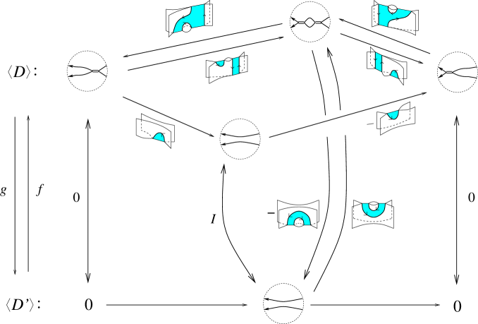
Figure 9. Invariance under $Reidemeister\ IIa$

• $g$ and $f$ are morphisms of complexes (use only isotopies);

• $g^{1}f^{1}=Id_{\langle D^{\prime}\rangle^{1}}$ (uses equation (55));

• $f^{0}g^{0}+hd=Id_{\langle D\rangle^{0}}$ and $f^{2}g^{2}+dh=Id_{\langle D\rangle^{2}}$ (use isotopies);

• $f^{1}g^{1}+dh+hd=Id_{\langle D\rangle^{1}}$ (use (DR₁)).

Reidemeister IIb: Consider diagrams $D$ and $D^{\prime}$ that differ only in a circular region, as in the figure below.

$$D=\raisebox{-13.0pt}{\includegraphics[height=28.90755pt]{DReidIIb.eps}}\qquad D^{\prime}=\raisebox{-13.0pt}{\includegraphics[height=28.90755pt]{twoedgesop.eps}}$$

Again, we sketch the arguments that the diagram in Figure 10 defines a homotopy equivalence between the complexes $\langle D\rangle$ and $\langle D^{\prime}\rangle$:

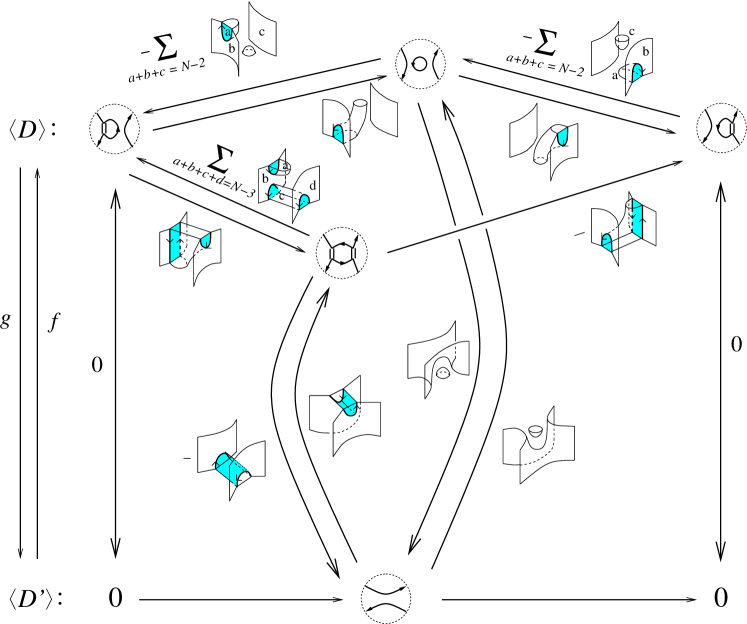
Figure 10. Invariance under $Reidemeister\ IIb$

• $g$ and $f$ are morphisms of complexes (use isotopies and DR₂);

• $g^{1}f^{1}=Id_{\langle D^{\prime}\rangle^{1}}$ (use (FC) and (S₁));

• $f^{0}g^{0}+hd=Id_{\langle D\rangle^{0}}$ and $f^{2}g^{2}+dh=Id_{\langle D\rangle^{2}}$ (use (RD₁) and (DR₂));

• $f^{1}g^{1}+dh+hd=Id_{\langle D\rangle^{1}}$ (use (DR₂), (RD₁), (3C) and (SqR₁)).

Reidemeister III: Consider diagrams $D$ and $D^{\prime}$ that differ only in a circular region, as in the figure below.

$$D=\raisebox{-13.0pt}{\includegraphics[height=28.90755pt]{D1ReidIII.eps}}\qquad D^{\prime}=\raisebox{-13.0pt}{\includegraphics[height=28.90755pt]{D2ReidIII.eps}}$$

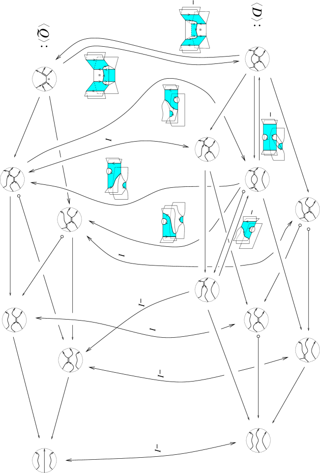
Figure 11. Invariance under $Reidemeister\ III$. A circle attached to the tail of an arrow indicates that the corresponding morphism has a minus sign.

In order to prove that $\langle D^{\prime}\rangle$ is homotopy equivalent to $\langle D\rangle$ we show that the latter is homotopy equivalent to a third complex denoted $\langle Q\rangle$ in Figure 11. The differential in $\langle Q\rangle$ in homological degree $0$ is defined by

for one summand and a similar foam for the other summand. By applying a symmetry relative to a horizontal axis crossing each diagram in $\langle D\rangle$ and $\langle Q\rangle$ we obtain a homotopy equivalence between $\langle D^{\prime}\rangle$ and $\langle Q^{\prime}\rangle$. It is easy to see that $\langle Q\rangle$ and $\langle Q^{\prime}\rangle$ are isomorphic. In homological degree $0$ the isomorphism is given by the obvious foam with two singular vertices. In the other degrees the isomorphism is given by the identity (in degrees $1$ and $2$ one has to swap the two terms of course). The fact that this defines an isomorphism follows immediately from the (MP) relation. We conclude that $\langle D\rangle$ and $\langle D^{\prime}\rangle$ are homotopy equivalent. ∎

From Theorem 7.1 we see that we can use any diagram $D$ of $L$ to obtain the invariant in $\mathbf{Kom}_{/h}(\mathbf{Foam}_{N})$ which justifies the notation $\langle L\rangle$ for $\langle D\rangle$.

8. Functoriality

The proof of the functoriality of our homology follows the same line of reasoning as in [1] and [9]. As in those papers, it is clear that the construction and the results of the previous sections can be extended to the category of tangles, following a similar approach using open webs and foams with corners. A foam with corners should be considered as living inside a cylinder, as in [1], such that the intersection with the cylinder is just a disjoint set of vertical edges.

The degree formula can be extended to the category of open webs and foams with corners by

Definition 8.1.

Let $u$ be a foam with $d$ dots of type , $d$ dots of type and $d$ dots of type . Let $b_{i}$ be the number of vertical edges of type $i$ of the boundary of $u$. The $q$-grading of $u$ is given by

(57) $$q(u)=-\sum_{i=1}^{3}i(N-i)q_{i}(u)-2(N-2)q_{\operatorname{s_{\gamma}}}(u)+\dfrac{1}{2}\sum_{i=1}^{3}i(N-i)b_{i}+2d+4d+6d.$$

Note that the Kapustin-Li formula also induces a grading on foams with corners, because for any foam $u$ between two (open) webs $\Gamma_{1}$ and $\Gamma_{2}$, it gives an element in the graded vector space $\mathop{\rm Ext}(M_{1},M_{2})$, where $M_{i}$ is the matrix factorization associated to $\Gamma_{i}$ in [6], for $i=1,2$. Recall that the $\mathop{\rm Ext}$ groups have a $\mathbb{Z}/2\mathbb{Z}\times\mathbb{Z}$-grading. For foams there is no $\mathbb{Z}/2\mathbb{Z}$-grading, but the $\mathbb{Z}$-grading survives.

Lemma 8.2.

For any foam $u$, the Kapustin-Li grading of $u$ is equal to $q(u)$.

Proof.

Both gradings are additive under horizontal and vertical glueing and are preserved by the relations in $\mathbf{Foam}_{N}$. Also the degrees of the dots are the same in both gradings. Therefore it is enough to establish the equality between the gradings for the foams which generate $\mathbf{Foam}_{N}$. For any foam without a singular graph the gradings are obviously equal, so let us concentrate on the singular cups and caps, the singular saddle point cobordisms and the cobordisms with one singular vertex in Figure 4. To compute the degree of the singular cups and caps, for both gradings, one can use the digon removal relations. For example, let us consider the singular cup

$$\raisebox{-10.0pt}{\includegraphics[height=28.90755pt]{scup.eps}}.$$

Any grading that preserves relation (DR₁) has to attribute the value of $-1$ to that foam, because the foam on the l.h.s. of (DR₁) has degree $0$, being an identity, and the dot on the r.h.s. has degree $2$. Similarly one can compute the degrees of the other singular cups and caps. To compute the degree of the singular saddle-point cobordisms, one can use the removing disc relations (RD₁) and (RD₂). For example, the saddle-point cobordism in Figure 4 has to have degree $1$. Finally, using the (MP) relation one shows that both foams on the r.h.s. in Figure 4 have to have degree $0$. ∎

Corollary 8.3.

For any closed foam $u$ we have that $\langle u\rangle_{KL}$ is zero if $q(u)\neq 0$.

As in [9] we have the following lemma, which is the analogue of Lemma 8.6 in [1]:

Lemma 8.4.

For a crossingless tangle diagram $T$ we have that $\mbox{Hom}_{\mathbf{Foam}_{N}}(T,T)$ is zero in negative degrees and $\mathbb{Q}$ in degree zero.

Proof.

Let $T$ be a crossingless tangle diagram and $u\in\mbox{Hom}_{\mathbf{Foam}_{N}}(T,T)$. Recall that $u$ can be considered to be in a cylinder with vertical edges intersecting the latter. The boundary of $u$ consists of a disjoint union of circles (topologically speaking). By dragging these circles slightly into the interior of $u$ one gets a disjoint union of circles in the interior of $u$. Apply relation (CN₁) to each of these circles. We get a linear combination of terms in $\mbox{Hom}_{\mathbf{Foam}_{N}}(T,T)$ each of which is the disjoint union of the identity on $T$, possibly decorated with dots, and a closed foam, which can be evaluated by $\langle\;\rangle_{KL}$. Note that the identity of $T$ with any number of dots has always non-negative degree. Therefore, if $u$ has negative degree, the closed foams above have negative degree as well and evaluate to zero. This shows the first claim in the lemma. If $u$ has degree $0$, the only terms which survive after evaluating the closed foams have degree $0$ as well and are therefore a multiple of the identity on $T$. This proves the second claim in the lemma. ∎

The proofs of Lemmas 8.7-8.9 in [1] are “identical”. The proofs of Theorem 4 and Theorem 5 follow the same reasoning but have to be adapted as in [9]. One has to use the homotopies of our Section 7 instead of the homotopies used in [1]. Without giving further details, we state the main result. Let $\mathbf{Kom}_{/\mathbb{Q}^{*}h}(\mathbf{Foam}_{N})$ denote the category $\mathbf{Kom}_{/h}(\mathbf{Foam}_{N})$ modded out by $\mathbb{Q}^{*}$, the invertible rational numbers. Then

Proposition 8.5.

$\langle\;\rangle$ defines a functor $\mathbf{Link}\rightarrow\mathbf{Kom}_{/\mathbb{Q}^{*}h}(\mathbf{Foam}_{N})$.

9. The $\ \mathfrak{sl}(N)$-link homology

Definition 9.1.

Let $\Gamma$, $\Gamma^{\prime}$ be closed webs and $f\in\mbox{Hom}_{\mathbf{Foam}_{N}}(\Gamma,\Gamma^{\prime})$. Define a functor $\mathcal{F}$ between the categories $\mathbf{Foam}_{N}$ and the category $\mathbf{Vect}_{\mathbb{Z}}$ of $\mathbb{Z}$-graded rational vector spaces and ${\mathbb{Z}}$-graded linear maps as

1. $\mathcal{F}(\Gamma)=\mbox{Hom}_{\mathbf{Foam}_{N}}(\emptyset,\Gamma),$

2. $\mathcal{F}(f)$ is the $\mathbb{Q}$-linear map $\mathcal{F}(f):\mbox{Hom}_{\mathbf{Foam}_{N}}(\emptyset,\Gamma)\rightarrow\mbox{Hom}_{\mathbf{Foam}_{N}}(\emptyset,\Gamma^{\prime})$ given by composition.

Note that $\mathcal{F}$ is a tensor functor and that the degree of $\mathcal{F}(f)$ equals $q(f)$. Note also that $\mathcal{F}(\unknot)\cong H^{*}\left(\mathbb{C}\mbox{P}^{N-1}\right)\{-N+1\}$ and $\mathcal{F}(\raisebox{-2.5pt}{\includegraphics[height=11.56346pt]{dble-circ.eps}})\cong H^{*}\left(\mathcal{G}_{2,N}\right)\{-2N+4\}$.

The following are a categorified version of the relations in Figure 3.

Lemma 9.2 (MOY decomposition).

We have the following decompositions under the functor $\mathcal{F}$:

1. $\mathcal{F}\left(\raisebox{-8.0pt}{\includegraphics[height=21.68121pt]{digon-up.eps}}\right)\cong\mathcal{F}\left(\raisebox{-8.0pt}{\includegraphics[height=21.68121pt]{dbedge-up.eps}}\right)\left\{-1\right\}\bigoplus\ \mathcal{F}\left(\raisebox{-8.0pt}{\includegraphics[height=21.68121pt]{dbedge-up.eps}}\right)\left\{1\right\}$.

2. $\mathcal{F}\left(\raisebox{-8.0pt}{\includegraphics[height=21.68121pt]{dbedge-dig.eps}}\right)\cong\bigoplus\limits_{i=0}^{N-2}\mathcal{F}\left(\raisebox{-8.0pt}{\includegraphics[height=21.68121pt]{edge-up.eps}}\right)\left\{2-N+2i\right\}$.

3. $\mathcal{F}\left(\raisebox{-8.0pt}{\includegraphics[height=21.68121pt]{square.eps}}\right)\cong\mathcal{F}\left(\raisebox{-8.0pt}{\includegraphics[height=21.68121pt]{twoedges-lr.eps}}\right)\bigoplus\left(\bigoplus\limits_{i=0}^{N-3}\ \mathcal{F}\left(\raisebox{-8.0pt}{\includegraphics[height=21.68121pt]{twoedges-ud.eps}}\right)\left\{3-N+2i\right\}\right)$.

4. $\mathcal{F}\left(\raisebox{-20.0pt}{\includegraphics[height=46.97505pt]{moy5-1.eps}}\right)\bigoplus\mathcal{F}\left(\raisebox{-20.0pt}{\includegraphics[height=46.97505pt]{moy5-21.eps}}\right)\cong\mathcal{F}\left(\raisebox{-20.0pt}{\includegraphics[height=46.97505pt]{moy5-2.eps}}\right)\bigoplus\mathcal{F}\left(\raisebox{-20.0pt}{\includegraphics[height=46.97505pt]{moy5-11.eps}}\right)$.

Proof.

(1): Define grading-preserving maps

$$\varphi_{0}:\mathcal{F}\left(\raisebox{-8.0pt}{\includegraphics[height=21.68121pt]{digon-up.eps}}\right)\left\{1\right\}\rightarrow\mathcal{F}\left(\raisebox{-8.0pt}{\includegraphics[height=21.68121pt]{dbedge-up.eps}}\right)\qquad\varphi_{1}:\mathcal{F}\left(\raisebox{-8.0pt}{\includegraphics[height=21.68121pt]{digon-up.eps}}\right)\left\{-1\right\}\rightarrow\mathcal{F}\left(\raisebox{-8.0pt}{\includegraphics[height=21.68121pt]{dbedge-up.eps}}\right)$$

$$\psi_{0}:\mathcal{F}\left(\raisebox{-8.0pt}{\includegraphics[height=21.68121pt]{dbedge-up.eps}}\right)\rightarrow\mathcal{F}\left(\raisebox{-8.0pt}{\includegraphics[height=21.68121pt]{digon-up.eps}}\right)\left\{1\right\}\qquad\psi_{1}:\mathcal{F}\left(\raisebox{-8.0pt}{\includegraphics[height=21.68121pt]{dbedge-up.eps}}\right)\rightarrow\mathcal{F}\left(\raisebox{-8.0pt}{\includegraphics[height=21.68121pt]{digon-up.eps}}\right)\left\{-1\right\}$$

as

$$\varphi_{0}=\mathcal{F}\left(\raisebox{-10.0pt}{\includegraphics[height=21.68121pt]{scap.eps}}\right),\ \ \ \varphi_{1}=\mathcal{F}\left(\raisebox{-10.0pt}{\includegraphics[height=21.68121pt]{scapd.eps}}\right),\ \ \ \psi_{0}=\mathcal{F}\left(\raisebox{-6.0pt}{\includegraphics[height=21.68121pt]{scupd.eps}}\right),\ \ \ \psi_{1}=-\mathcal{F}\left(\raisebox{-6.0pt}{\includegraphics[height=21.68121pt]{scup.eps}}\right).$$

The bubble identities imply that $\varphi_{i}\psi_{j}=\delta_{i,j}$ (for $i,j=0,1$) and from the (DR₁) relation it follows that $\psi_{0}\varphi_{0}+\psi_{1}\varphi_{1}$ is the identity map in $\mathcal{F}\left(\raisebox{-5.0pt}{\includegraphics[height=14.45377pt]{digon-l.eps}}\right)$.

(2): Define grading-preserving maps

$$\varphi_{i}:\mathcal{F}\left(\raisebox{-8.0pt}{\includegraphics[height=21.68121pt]{dbedge-dig.eps}}\right)\left\{N-2-2i\right\}\rightarrow\mathcal{F}\left(\raisebox{-8.0pt}{\includegraphics[height=21.68121pt]{edge-up.eps}}\right),\qquad\psi_{i}:\mathcal{F}\left(\raisebox{-8.0pt}{\includegraphics[height=21.68121pt]{edge-up.eps}}\right)\rightarrow\mathcal{F}\left(\raisebox{-8.0pt}{\includegraphics[height=21.68121pt]{dbedge-dig.eps}}\right)\left\{N-2-2i\right\},$$

for $0\leq i\leq N-2$, as

$$\varphi_{i}=\mathcal{F}\left(\raisebox{-24.0pt}{\includegraphics[height=46.97505pt]{scap_b-N2i.eps}}\right),\qquad\psi_{i}=\sum\limits_{j=0}^{i}\mathcal{F}\left(\raisebox{-22.0pt}{\includegraphics[height=46.97505pt]{scup_b-iij.eps}}\right).$$

We have $\varphi_{i}\psi_{k}=\delta_{i,k}$ and $\sum\limits_{i=0}^{N-2}\psi_{i}\varphi_{i}=Id\left(\mathcal{F}\left(\raisebox{-4.0pt}{\includegraphics[height=14.45377pt]{dbedge-dig-l.eps}}\right)\right)$. The first assertion is straightforward and can be checked using the (RD) and (S₁) relations and the second is immediate from the (DR₂) relation, which can be written as

$$\raisebox{-32.0pt}{\includegraphics[height=57.81621pt]{digonfid_b.eps}}=\sum_{i=0}^{N-2}\sum_{j=0}^{i}\ \raisebox{-32.0pt}{\includegraphics[height=57.81621pt]{dig_rem_b-ij.eps}}\hbox to0.0pt{\hskip 64.58313pt\text{(DR${}_{2}$)}\hss}$$

(3): Define grading-preserving maps

$$\varphi_{i}:\mathcal{F}\left(\raisebox{-8.0pt}{\includegraphics[height=21.68121pt]{square.eps}}\right)\left\{N-3+2i\right\}\rightarrow\mathcal{F}\left(\raisebox{-8.0pt}{\includegraphics[height=21.68121pt]{twoedges-ud.eps}}\right),\quad\psi_{i}:\mathcal{F}\left(\raisebox{-8.0pt}{\includegraphics[height=21.68121pt]{twoedges-ud.eps}}\right)\rightarrow\mathcal{F}\left(\raisebox{-8.0pt}{\includegraphics[height=21.68121pt]{square.eps}}\right)\left\{N-3+2i\right\},$$

for $0\leq i\leq N-3$, and

$$\rho:\mathcal{F}\left(\raisebox{-8.0pt}{\includegraphics[height=21.68121pt]{square.eps}}\right)\rightarrow\mathcal{F}\left(\raisebox{-8.0pt}{\includegraphics[height=21.68121pt]{twoedges-lr.eps}}\right),\qquad\tau:\mathcal{F}\left(\raisebox{-8.0pt}{\includegraphics[height=21.68121pt]{twoedges-lr.eps}}\right)\rightarrow\mathcal{F}\left(\raisebox{-8.0pt}{\includegraphics[height=21.68121pt]{square.eps}}\right),$$

as

$$\varphi_{i}=\mathcal{F}\left(\raisebox{-22.0pt}{\includegraphics[height=50.58878pt]{hcylhalf-bot-i.eps}}\right),\qquad\psi_{i}=\sum\limits_{a+b+c=N-3-i}\mathcal{F}\left(\raisebox{-22.0pt}{\includegraphics[height=50.58878pt]{hcylhalf-top-abc.eps}}\right),$$

$$\rho=\mathcal{F}\left(\raisebox{-22.0pt}{\includegraphics[height=50.58878pt]{hdcylhalf-bot.eps}}\right),\qquad\tau=-\mathcal{F}\left(\raisebox{-22.0pt}{\includegraphics[height=50.58878pt]{hdcylhalf-top.eps}}\right).$$

Checking that $\varphi_{i}\psi_{k}=\delta_{i,k}$ for $0\leq i,k\leq N-3$, $\varphi_{i}\tau=0$ and $\rho\psi_{i}=0$, for $0\leq i\leq N-3$, and $\rho\tau=-1$ is left to the reader. From the (SqR₁) relation it follows that $\tau\rho+\sum\limits_{i=0}^{N-3}\psi_{i}\varphi_{i}=Id\left(\mathcal{F}\left(\raisebox{-4.5pt}{\includegraphics[height=14.45377pt]{square.eps}}\right)\right)$.

Direct Sum Decomposition (4): We prove direct decomposition (4) showing that

Note that this suffices because the last term on the r.h.s. of a) is isomorphic to the last term on the r.h.s. of b) by the (MP) relation.

To prove $a)$ we define grading-preserving maps

$$\varphi_{0}:\mathcal{F}\left(\raisebox{-15.0pt}{\includegraphics[height=36.135pt]{moy5-1.eps}}\right)\rightarrow\mathcal{F}\left(\raisebox{-15.0pt}{\includegraphics[height=36.135pt]{moy5-11.eps}}\right),\qquad\varphi_{1}:\mathcal{F}\left(\raisebox{-15.0pt}{\includegraphics[height=36.135pt]{moy5-1.eps}}\right)\rightarrow\mathcal{F}\left(\raisebox{-15.0pt}{\includegraphics[height=36.135pt]{moy5-22.eps}}\right),$$

$$\psi_{0}:\mathcal{F}\left(\raisebox{-15.0pt}{\includegraphics[height=36.135pt]{moy5-11.eps}}\right)\rightarrow\mathcal{F}\left(\raisebox{-15.0pt}{\includegraphics[height=36.135pt]{moy5-1.eps}}\right),\qquad\psi_{1}:\mathcal{F}\left(\raisebox{-15.0pt}{\includegraphics[height=36.135pt]{moy5-22.eps}}\right)\rightarrow\mathcal{F}\left(\raisebox{-15.0pt}{\includegraphics[height=36.135pt]{moy5-1.eps}}\right),$$

by

$$\varphi_{0}=-\mathcal{F}\left(\raisebox{-19.0pt}{\includegraphics[height=43.36243pt]{hcylhalf_b.eps}}\right),\qquad\varphi_{1}=-\mathcal{F}\left(\raisebox{-19.0pt}{\includegraphics[height=43.36243pt]{hdighalf_b.eps}}\right),$$

$$\psi_{0}=\mathcal{F}\left(\raisebox{-19.0pt}{\includegraphics[height=43.36243pt]{hcylhalf_t.eps}}\right),\qquad\psi_{1}=\mathcal{F}\left(\raisebox{-19.0pt}{\includegraphics[height=43.36243pt]{hdighalf_t.eps}}\right).$$

We have that $\varphi_{i}\psi_{j}=\delta_{i,j}$ for $i,j=0,1$ (we leave the details to the reader). From the (SqR₂) relation it follows that

$$\psi_{0}\varphi_{0}+\psi_{1}\varphi_{1}=Id\left(\mathcal{F}\left(\raisebox{-15.0pt}{\includegraphics[height=36.135pt]{moy5-1.eps}}\right)\right).$$

Applying a symmetry to all diagrams in decomposition $a)$ gives us decomposition $b)$. ∎

In order to relate our construction to the $\mathfrak{sl}(N)$ polynomial we need to introduce shifts. We denote by $\{n\}$ an upward shift in the $q$-grading by $n$ and by $[m]$ an upward shift in the homological grading by $m$.

Definition 9.3.

Let $\langle L\rangle_{i}$ denote the $i$-th homological degree of the complex $\langle L\rangle$. We define the $i$-th homological degree of the complex $\mathcal{F}(L)$ to be

$$\mathcal{F}_{i}(L)=\mathcal{F}\langle L\rangle_{i}[-n_{-}]\{(N-1)n_{+}-Nn_{-}+i\},$$

where $n_{+}$ and $n_{-}$ denote the number of positive and negative crossings in the diagram used to calculate $\langle L\rangle$.

We now have a homology functor $\mathbf{Link}\rightarrow\mathbf{Vect}_{\mathbb{Z}}$ which we still call $\mathcal{F}$. Definition 9.3, Theorem 7.1 and Lemma 9.2 imply that

Theorem 9.4.

For a link $L$ the graded Euler characteristic of $H^{*}\left(\mathcal{F}(L)\right)$ equals $P_{N}(L)$, the $\mathfrak{sl}(N)$ polynomial of $L$.

The MOY-relations are also the last bit that we need in order to show the following theorem.

Theorem 9.5.

For any link $L$, the bigraded complex $\mathcal{F}(L)$ is isomorphic to the Khovanov-Rozansky complex $KR(L)$ in [6].

Proof.

The map $\langle\ |_{KL}$ defines a grading preserving linear injection $\mathcal{F}(\Gamma)\to KR(\Gamma)$, for any web $\Gamma$. Lemma 9.2 implies that the graded dimensions of $\mathcal{F}(\Gamma)$ and $KR(\Gamma)$ are equal, so $\langle\ |_{KL}$ is a grading preserving linear isomorphism, for any web $\Gamma$.

To prove the theorem we would have to show that $\langle\ |_{KL}$ commutes with the differentials. We call

      

the zip and

      

the unzip. Note that both the zip and the unzip have $q$-degree $1$. Let $\Gamma_{1}$ be the source web of the zip and $\Gamma_{2}$ its target web, and let $\Gamma$ be the theta web, which is the total boundary of the zip where the vertical edges have been pinched. The $q$-dimension of $\mathop{\rm Ext}(\Gamma_{1},\Gamma_{2})$ is equal to

$$q^{2N-2}\mathop{\rm qdim}(\Gamma)=q+q^{2}(\ldots),$$

where $(\ldots)$ is a polynomial in $q$. Therefore the differentials in the two complexes commute up to a scalar. By the removing disc relation (RD₁) we see that if the “zips” commute up to $\lambda$, then the “unzips” commute up to $\lambda^{-1}$. If $\lambda\neq 1$, we have to modify our map between the two complexes slightly, in order to get an honest morphism of complexes. We use Khovanov’s idea of “twist equivalence” in [4]. For a given link consider the hypercube of resolutions. If an arrow in the hypercube corresponds to a zip, multiply $\langle(\mbox{target})|_{KL}$ by $\lambda$, where target means the target of the arrow. If it corresponds to an unzip, multiply $\langle(\mbox{target})|_{KL}$ by $\lambda^{-1}$. This is well-defined, because all squares in the hypercube (anti-)commute. By definition this new map commutes with the differentials and therefore proves that the two complexes are isomorphic. ∎

We conjecture that the above isomorphism actually extends to link cobordisms, giving a projective natural isomorphism between the two projective link homology functors. Proving this would require a careful comparison between the two functors for all the elementary link cobordisms.

Acknowledgements The authors thank Mikhail Khovanov for helpful comments and Lev Rozansky for patiently explaining the Kapustin-Li formula in detail to us.

The authors were supported by the Fundação para a Ciência e a Tecnologia (ISR/IST plurianual funding) through the programme “Programa Operacional Ciência, Tecnologia, Inovação” (POCTI) and the POS Conhecimento programme, cofinanced by the European Community fund FEDER.

References

- [1] D. Bar-Natan, Khovanov’s homology for tangles and cobordisms, Geom. Topol. 9: 1443-1499, 2005.
- [2] W. Fulton and J. Harris, Representation theory, A first course, Graduate Texts in Mathematics, 129. Readings in Mathematics. Springer-Verlag, New York, 1991.
- [3] M. Khovanov, link homology, Alg. Geom. Top. 4: 1045-1081, 2004.
- [4] M. Khovanov, Link homology and Frobenius extensions, Fund. Math. 190: 179-190 , 2006.
- [5] A. Kapustin and Y. Li, Topological correlators in Landau-Ginzburg models with boundaries, Adv. Theor. Math. Phys. 7: 727-749, 2003.
- [6] M. Khovanov and L. Rozansky, Matrix factorizations and link homology, preprint 2004, arXiv: math. QA/0401268.
- [7] M. Khovanov and L. Rozansky, Topological Landau-Ginzburg models on a world-sheet foam, Adv. Theor. Math. Phys. 11: 233-260, 2007.
- [8] M. Khovanov and L. Rozansky, Virtual crossings, convolutions and a categorification of the Kauffman polynomial, preprint 2007, arXiv: math.QA/0701333
- [9] M. Mackaay and P. Vaz, The universal -link homology, Algebr. Geom. Topol. 7 (2007) 1135-1169.
- [10] H. Murakami, T. Ohtsuki, S. Yamada, HOMFLY polynomial via an invariant of colored plane graphs, Enseign. Math. (2) 44: 325-360, 1998.
- [11] L. Rozansky, Topological A-models on seamed Riemann surfaces, preprint 2003, arXiv: hep-th/0305205.