Squeezed-light generation in a nonlinear planar waveguide with a periodic corrugation

Abstract

Two-mode nonlinear interaction (second-harmonic and second-subharmonic generation) in a planar waveguide with a small periodic corrugation at the surface is studied. Scattering of the interacting fields on the corrugation leads to constructive interference that enhances the nonlinear process provided that all the interactions are phase matched. Conditions for the overall phase matching are found. Compared with a perfectly quasi-phase-matched waveguide, better values of squeezing as well as higher intensities are reached under these conditions. Procedure for finding optimum values of parameters for squeezed-light generation is described.

I Introduction

Since the pioneering work by Armstrong Armstrong1962 on the process of second-harmonic generation has occurred, spatio-temporal properties of the nonlinearly interacting classical fields have been studied in detail by many authors both theoretically and experimentally. A new impulse in these studies has occurred when people understood that this process can give rise to the fields with nonclassical properties (for a review, see, e.g. Perina1991 ). Namely light with electric-field amplitude fluctuations suppressed below the limit given by quantum mechanics can be generated both in the pump and second-subharmonic fields. Also light with nonclassical photon-number statistics can be obtained - pairwise character of photon-number statistics Schleich1987 ; Perina1990 generated in the spontaneous process of second-subharmonic generation has been observed Waks2004 .

It has been shown that the best conditions for squeezed-light generation in homogeneous nonlinear media occur, provided that the nonlinear two-mode interaction is perfectly phase matched. Under these conditions, the principal squeeze variance of the second-subharmonic field can asymptotically reach zero when the gain of the nonlinear interaction increases. On the other hand, the pump-field principal squeeze variance cannot be less than 0.5 Ou1994 . If large values of the nonlinear phase mismatch are allowed, this limit can be overcome due to a nonlinear phase modulation, as suggested in Li1993 ; Li1994 . However, the generated signal is very weak.

The most common method how to compensate for the natural nonlinear phase mismatch that occurs in commonly used nonlinear materials is to introduce an additional periodic modulation of the $\chi^{(2)}$ susceptibility using periodical poling Serkland1995 ; Serkland1997 ; Yu2005 . Several methods for the additional modulation of the local amplitude of this quasi-phase-matched interaction have been developed Huang2006 . These methods allow to reach a spectrally broad-band two-mode interaction and so femtosecond pumping of the nonlinear process is possible Schober2005 .

In order to effectively increase low values of the nonlinear interaction in real materials, configurations in which a nonlinear medium is put inside a cavity are usually used to generate squeezed light (e.g. Lawrence2002 ; Leonhardt1997 ; Bachor2004 ).

In a waveguiding geometry that profits from a strong spatial confinement of the interacting optical fields in the transverse plane resulting in high values of the effective nonlinearity, another method to reach a nonlinear phase mismatch is possible. One of the nonlinearly interacting fields can be coupled through its evanescent waves into another field of the same frequency propagating in a neighbouring waveguide. An exchange of energy between these two linearly coupled fields introduces a spatial modulation of the nonlinearly interacting field that can be set to compensate for the nonlinear phase mismatch Dong2004 . Interaction of fields in different waveguides through their evanescent waves can be used in various configurations that modify nonclassical properties of optical fields emerging from nonlinear interactions PerinaJr2000 .

A waveguiding geometry allows another possibility to tailor the nonlinear process - a linear periodic corrugation of the waveguide surface can be introduced as a distributed feedback that scatters the propagating fields Joannopoulos1995 ; Bertolotti2001 . Under suitable conditions, the scattered contributions interfere constructively and increase electric-field amplitudes of the propagating fields. This then results in higher conversion efficiencies of the nonlinear process Haus1998 ; Pezzetta2001 . Also squeezed-light generation is supported in this geometry, as discussed in Tricca2004 where scattering of the second-harmonic field on the corrugation has been neglected. A waveguiding geometry with a periodic corrugation can also be conveniently used for second-harmonic generation in Čerenkov configuration Pezzetta2002 . A general model of squeezed-light generation in nonlinear photonic structures has been developed in Sakoda2002 .

In this paper, we show that scattering of the interacting fields caused by a linear periodic corrugation supports the generation of squeezed light in both the pump and second-subharmonic fields provided that an electric-field amplitude of at least one of the interacting fields is increased inside the waveguide as a consequence of scattering. We note that an increase of electric-field amplitudes in the area of periodic corrugation is small compared with that occurring in layered photonic band-gap structures (with a deep grating) Scalora1997 ; DAguanno2001 ; Dumeige2001 .

The generation of squeezed light has been in the center of attention in quantum optics for more than twenty years. It has been shown that the squeezed light can be generated also in Kerr media, nonlinear process of four-wave mixing, and diode lasers pumped by a sub-Poissonian current (for a review, see Bachor2004 ). The level of squeezing observable in recent experiments Takeno2007 ; Vahlbruch2007 approaches 10 dB below the shot-noise level.

The paper is organized as follows. In Sec. II, a quantum model of the nonlinear interaction including both Heisenberg equations for operator electric-field amplitudes and model of a generalized superposition of signal and noise are presented. Conditions for an efficient squeezed-light generation are derived in Sec. III. A detailed analysis of the waveguide made of LiNbO₃ is contained in Sec. IV. Conclusions are drawn in Sec. V. Appendix A is devoted to mode analysis of an anisotropic planar waveguide.

II Model of the nonlinear interaction

An overall electric-field amplitude ${\bf E}({\bf r},t)$ describing an optical field in the considered anisotropic nonlinear waveguide (shown in Fig. 1) is composed of two contributions; pump (or fundamental) electric-field amplitude ${\bf E}_{p}({\bf r},t)$ at frequency $\omega$ and second-subharmonic electric-field amplitude ${\bf E}_{s}({\bf r},t)$ at frequency $\omega/2$; i.e. ${\bf E}={\bf E}_{p}+{\bf E}_{s}$. We note that in case of second-harmonic generation, the field with the amplitude ${\bf E}_{p}({\bf r},t)$ is called second-harmonic and that with the amplitude ${\bf E}_{s}({\bf r},t)$ is known as pump. We keep the terminology used for second-subharmonic generation throughout the paper.

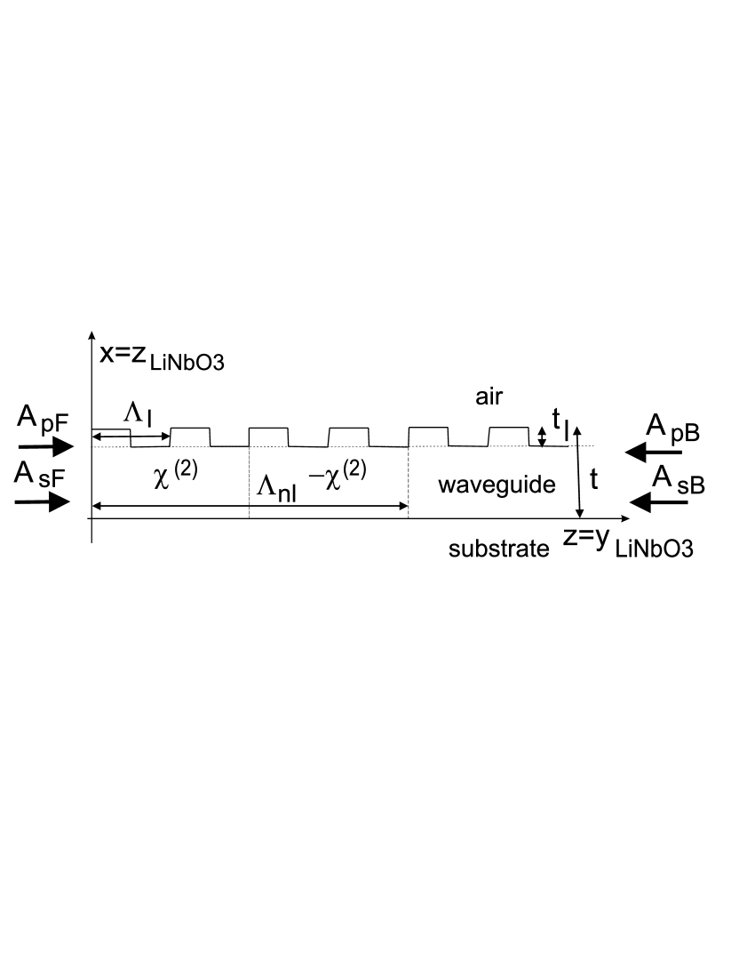
Figure 1: Four optical fields interact in a nonlinear waveguide of thickness $t$ and length $L$ with a periodically-poled (period $\Lambda_{nl}$) $\chi^{(2)}$ susceptibility; $A_{p_{F}}$, $A_{p_{B}}$, $A_{s_{F}}$, and $A_{s_{B}}$ mean forward-propagating pump, backward-propagating pump, forward-propagating second-subharmonic, and backward-propagating second-subharmonic electric-field amplitudes, respectively. A linear corrugation with depth $t_{l}$ and period $\Lambda_{l}$ is fabricated on the waveguide upper surface. Profile of the waveguide in the $x-y$ plane is rectangular with width $\Delta y$ and depth $t$; $\Delta y\gg t$ is assumed. The waveguide is made of LiNbO₃ with the optical axis oriented along the $x$ axis.

The electric-field amplitude ${\bf E}$ obeys the wave equation inside the waveguide with a nonlinear source term Snyder1983 ; Haus1984 :

$$\Delta{\bf E}-\nabla(\nabla\cdot{\bf E})-\mu\epsilon_{0}{\bf\epsilon}\cdot\frac{\partial^{2}{\bf E}}{\partial t^{2}}=\mu\frac{\partial^{2}{\bf P}_{\rm nl}}{\partial t^{2}}.$$ (1)

In Eq. (1) $\mu$ denotes vacuum permeability, $\epsilon_{0}$ vacuum permittivity, and ${\bf P}_{\rm nl}$ describes nonlinear polarization of the medium. The symbol $\Delta$ stands for Laplace operator, $(\cdot)$ means a scalar product, and $\cdot$ denotes tensorial multiplication. Every spectral component of the element ${\bf\epsilon}_{ij}({\bf r},\omega)$ of the relative permittivity tensor in the considered waveguide can be expressed as follows:

$${\bf\epsilon}_{ij}(x,y,z,\omega)=\bar{\bf\epsilon}_{ij}(x,y,\omega)\left[1+\Delta\epsilon_{ij}(x,y,z,\omega)\right].$$ (2)

Small variations of permittivity ${\bf\epsilon}$ described by $\Delta\epsilon_{ij}(x,y,z,\omega)$ are induced by a periodic corrugation of the waveguide surface. These variations of the elements $\Delta\epsilon_{ij}(x,y,z,\omega)$ along the z axis can be conveniently decomposed into harmonic waves:

$$\Delta\epsilon_{ij}(x,y,z,\omega)=\sum_{q=-\infty}^{\infty}{\bf\varepsilon}_{ij,q}(x,y,\omega)\exp\left[iq\frac{2\pi}{\Lambda_{l}}z\right],$$ (3)

where ${\bf\varepsilon}_{q,ij}$ are coefficients of the decomposition and $\Lambda_{l}$ is a period of the linear corrugation. Amplitude of the nonlinear polarization ${\bf P}_{\rm nl}$ of the medium is determined using tensor ${\bf d}$ of the second-order nonlinear coefficient:

$${\bf P}_{\rm nl}({\bf r},t)=2\epsilon_{0}{\bf d}({\bf r})\cdot{\bf E}({\bf r},t){\bf E}({\bf r},t).$$ (4)

Taking into account geometry of our waveguide elements ${\bf d}_{ijk}({\bf r})$ of the nonlinear coefficient can be expressed as follows:

$${\bf d}_{ijk}(x,y,z)=\sum_{q=-\infty}^{\infty}{\bf d}_{ijk,q}(x,y)\exp\left[iq\frac{2\pi}{\Lambda_{nl}}z\right],$$ (5)

where $\Lambda_{nl}$ describes the period of a possible periodical poling of the nonlinear material.

The electric-field amplitudes of pump (${\bf E}_{p}$) and second-subharmonic (${\bf E}_{s}$) monochromatic waves can be expressed in the form:

$${\bf E}_{a}(x,y,z,t) = i\left[A_{a_{F}}(z){\bf e}_{a}(x,y)\exp(i\beta_{a}z-i\omega_{a}t)\right.$$ (6)

$$\mbox{}+A_{a_{B}}(z){\bf e}_{a}(x,y)\exp(-i\beta_{a}z-i\omega_{a}t)$$

$$\mbox{}\left.-{\rm H.c.}\right],\hskip 28.45274pta=p,s,$$

where the symbols ${\bf e}_{p}$ and ${\bf e}_{s}$ refer to mode functions in the transverse plane of the beams. Amplitudes $A_{p_{F}}$ and $A_{s_{F}}$ [$A_{p_{B}}$ and $A_{s_{B}}$] describe forward- [backward-] propagating pump and second-subharmonic fields and are such that the quantities $|A_{p_{F}}|^{2}$, $|A_{p_{B}}|^{2}$, $|A_{s_{F}}|^{2}$, and $|A_{s_{B}}|^{2}$ give directly the number of photons in these fields. Symbol $\beta_{a}$ means propagation constant along the z axis in mode $a$ whereas $\omega_{a}$ stands for frequency of this mode. Symbol ${\rm H.c.}$ replaces hermitian conjugated terms. We note that the considered anisotropic waveguide supports only TM guided modes; TE modes are not guided and thus do not contribute significantly to nonlinear interaction.

Mode functions ${\bf e}_{p}$ and ${\bf e}_{s}$ describe the transverse profiles of pump and second-subharmonic fields, respectively, and fulfill the following equations:

$$\nabla\times\left(\nabla\times\left[{\bf e}_{a}(x,y)\exp(\pm i\beta_{a}z-i\omega_{a}t)\right]\right)$$

$$\mbox{}-\frac{\omega_{s}^{2}}{c^{2}}\bar{\bf\epsilon}_{ij}(x,y,\omega_{a})\cdot\left[{\bf e}_{a}(x,y)\exp(\pm i\beta_{a}z-i\omega_{a}t)\right]=0,$$

$$\hskip 85.35826pta=p,s.$$ (7)

We note that mean values of permittivities $\bar{\bf\epsilon}_{ij}(x,y,\omega_{a})$ are used for the determination of mode functions. The mode functions ${\bf e}_{p}$ and ${\bf e}_{s}$ are normalized to describe one photon in a mode inside the waveguide (see Appendix A).

Substitution of Eqs. (2-6) into Eq. (1) assuming $\left|\frac{\partial^{2}A_{a_{b}}}{\partial z^{2}}\right|\ll\left|\beta_{a}\frac{\partial A_{a_{b}}}{\partial z}\right|$ for $a=p,s$ and $b=F,B$ (analog of the slowly-varying envelope approximation to spatial evolution) results in the following equations for amplitudes $A_{p_{F}}$, $A_{p_{B}}$, $A_{s_{F}}$, and $A_{s_{B}}$:

$$\frac{dA_{s_{F}}}{dz} = iK_{s}\exp(-i\delta_{s}z)A_{s_{B}}$$

$$\mbox{}+4K_{nl,q}\exp(i\delta_{nl,q}z)A_{p_{F}}A^{*}_{s_{F}},$$

$$\frac{dA_{s_{B}}}{dz} = -iK^{*}_{s}\exp(i\delta_{s}z)A_{s_{F}}$$

$$\mbox{}-4K_{nl,q}\exp(-i\delta_{nl,q}z)A_{p_{B}}A^{*}_{s_{B}},$$

$$\frac{dA_{p_{F}}}{dz} = iK_{p}\exp(-i\delta_{p}z)A_{p_{B}}$$

$$\mbox{}-2K^{*}_{nl,q}\exp(-i\delta_{nl,q}z)A_{s_{F}}^{2},$$

$$\frac{dA_{p_{B}}}{dz} = -iK_{p}^{*}\exp(i\delta_{p}z)A_{p_{F}}$$ (8)

$$\mbox{}+2K^{*}_{nl,q}\exp(i\delta_{nl,q}z)A_{s_{B}}^{2}.$$

Because the waveguide is made of an anisotropic material, also the following relation has to hold in order to derive correctly equations in Eq. (8) (for details, see Snyder1983 ):

$$\frac{d^{2}A_{a_{b}}(z)}{dz^{2}}[{\bf e}_{a}(x,y)]_{z}\exp(\pm i\beta_{a}z)\;{\bf z}$$

$$\mbox{}+\frac{dA_{a_{b}}(z)}{dz}\nabla\left([{\bf e}_{a}(x,y)]_{z}\exp(\pm i\beta_{a}z)\right)$$

$$\mbox{}+\frac{dA_{a_{b}}(z)}{dz}\left(\nabla\cdot\left[{\bf e}_{a}(x,y)\exp(\pm i\beta_{a}z)\right]\right)\;{\bf z}\approx 0,$$

$$\hskip 85.35826pta=p,s,\hskip 8.53581ptb=F,B,$$ (9)

and ${\bf z}$ stands for a unit vector along the $z$ axis. We note that Eqs. (8) describe also a nonlinear coupler composed of two waveguides made of $\chi^{(2)}$ media whose modes interact through evanescent waves. Nonclassical properties of light propagating in this coupler have been studied in Perina1996 ; Korolkova1997 . A scheme that allows to decompose interactions in this coupler into a sequence of fictitious interactions has been suggested in Fiurasek2000 .

Phase mismatches $\delta_{s}$, $\delta_{p}$, and $\delta_{nl,q}$ occurring in Eq. (8) are given as follows:

$$\delta_{a} = 2\beta_{a}-\frac{2\pi}{\Lambda_{l}},\hskip 8.53581pta=p,s,$$

$$\delta_{nl,q} = \beta_{p}-2\beta_{s}+q\frac{2\pi}{\Lambda_{nl}}.$$ (10)

Coefficient $q$ equals $\pm 1$ for a periodically poled nonlinear material, whereas $q=0$ for a material without periodical poling. Linear coupling constants $K_{p}$ and $K_{s}$ are determined along the expressions:

$$K_{a} = \frac{\omega_{a}^{2}}{2c^{2}\beta_{a}}\frac{\int dxdy\,{\bf\varepsilon}_{1}(x,y,\omega_{a})\cdot{\bf e}^{*}_{a}(x,y){\bf e}_{a}(x,y)}{\int dxdy\,|{\bf e}_{a}(x,y)|^{2}},$$ (11)

$$a=p,s.$$

Similarly, the following expression can be found for nonlinear coupling constants $K_{nl,q}$ for $q=0,\pm 1$:

$$K_{nl,q} = \frac{2i\omega_{s}^{2}}{c^{2}\beta_{s}}\frac{\int dxdy\,{\bf d}_{q}(x,y)\cdot{\bf e}_{p}(x,y){\bf e}^{*}_{s}(x,y){\bf e}^{*}_{s}(x,y)}{\int dxdy\,|{\bf e}_{s}(x,y)|^{2}}$$

$$\approx \frac{2i\omega_{p}^{2}}{c^{2}\beta_{p}}\frac{\int dxdy\,{\bf d}_{q}(x,y)\cdot{\bf e}_{p}(x,y){\bf e}^{*}_{s}(x,y){\bf e}^{*}_{s}(x,y)}{\int dxdy\,|{\bf e}_{p}(x,y)|^{2}}.$$

The last approximate equality in Eq. (LABEL:12) is valid provided that $\omega_{s}/\beta_{s}\approx\omega_{p}/\beta_{p}$ and due to the normalization of the mode functions ${\bf e}_{s}$ and ${\bf e}_{p}$. This approximation assures, that only one nonlinear coupling constant occurs in Eqs. (8) which is important in quantum description.

Expressions for linear ($K_{s}$, $K_{p}$) and nonlinear ($K_{nl,0}$, $K_{nl,1}$) coupling constants appropriate for the considered waveguide and derived from Eqs. (11) and (LABEL:12) can be found in Appendix A in Eqs. (59-61).

Quantum model of the nonlinear interaction in the considered waveguide can be formulated changing the classical envelope electric-field amplitudes $A_{p_{F}}$, $A_{p_{B}}$, $A_{s_{F}}$, and $A_{s_{B}}$ occurring in Eq. (6) into operators denoted as $\hat{A}_{p_{F}}$, $\hat{A}_{p_{B}}$, $\hat{A}_{s_{F}}$, and $\hat{A}_{s_{B}}$, respectively. A quantum analog of the classical equations written in Eq. (8) can then be derived from the Heisenberg equations (for details, see PerinaJr2004 ; PerinaJr2005 ;

$$\frac{d\hat{X}}{dz}=-\frac{i}{\hbar}\left[\hat{G},\hat{X}\right];$$ (13)

considering the following momentum operator $\hat{G}$:

$$\hat{G} = \left[\hbar K_{s}\exp(-i\delta_{s}z)\hat{A}^{\dagger}_{s_{F}}\hat{A}_{s_{B}}\right.$$ (14)

$$\mbox{}\left.+\hbar K_{p}\exp(-i\delta_{p}z)\hat{A}^{\dagger}_{p_{F}}\hat{A}_{p_{B}}+{\rm H.c.}\right]$$

$$-\left[2i\hbar K_{nl,q}\exp(i\delta_{nl,q}z)\hat{A}^{\dagger 2}_{s_{F}}\hat{A}_{p_{F}}\right.$$

$$\mbox{}\left.+2i\hbar K_{nl,q}\exp(-i\delta_{nl,q}z)\hat{A}^{\dagger 2}_{s_{B}}\hat{A}_{p_{B}}+{\rm H.c.}\right],$$

where $q=0$ or $q=\pm 1$. In Eq. (13), $\hbar$ means the reduced Planck constant, $\hat{X}$ stands for an arbitrary operator and the symbol $[,]$ denotes commutator.

The operator quantum equations analogous to those written in Eq. (8) can be solved using the method of a small operator correction (denoted as $\delta\hat{A}$) to a mean value (denoted as $A$) in which an operator electric-field amplitude $\hat{A}$ is decomposed as $\hat{A}=A+\delta\hat{A}$. This method provides a set of classical nonlinear equations for the mean values $A$ that coincides with the set given in Eq. (8). The operator electric-field amplitude corrections $\delta\hat{A}$ fulfill the following linear operator equations:

$$\frac{d\delta\hat{A}_{s_{F}}}{dz} = {\cal K}_{s}\delta\hat{A}_{s_{B}}+{\cal K}_{F,q}\left[A_{p_{F}}\delta\hat{A}^{\dagger}_{s_{F}}+A^{*}_{s_{F}}\delta\hat{A}_{p_{F}}\right],$$

$$\frac{d\delta\hat{A}_{s_{B}}}{dz} = {\cal K}^{*}_{s}\delta\hat{A}_{s_{F}}-{\cal K}_{B,q}\left[A_{p_{B}}\delta\hat{A}^{*}_{s_{B}}+A^{*}_{s_{B}}\delta\hat{A}_{p_{B}}\right],$$

$$\frac{d\delta\hat{A}_{p_{F}}}{dz} = {\cal K}_{p}\delta\hat{A}_{p_{B}}-{\cal K}^{*}_{F,q}A_{s_{F}}\delta\hat{A}_{s_{F}},$$

$$\frac{d\delta\hat{A}_{p_{B}}}{dz} = {\cal K}^{*}_{p}\delta\hat{A}_{p_{B}}+{\cal K}^{*}_{B,q}A_{s_{B}}\delta\hat{A}_{s_{B}}.$$ (15)

The functions ${\cal K}_{s}$, ${\cal K}_{p}$, and ${\cal K}_{nl,q}$ introduced in Eqs. (15) are defined as:

$${\cal K}_{a} = iK_{a}\exp(-i\delta_{a}z),\hskip 28.45274pta=s,p,$$

$${\cal K}_{F,q} = 4K_{nl,q}\exp(i\delta_{nl,q}z),$$

$${\cal K}_{B,q} = 4K_{nl,q}\exp(-i\delta_{nl,q}z).$$ (16)

Solution of the classical nonlinear equations written in Eqs. (8) can only be reached numerically using, e.g., a finite difference method called BVP NumericalRecipes . This method requires an initial guess of the solution that can be conveniently obtained when the nonlinear terms in Eqs. (8) are omitted. Then, the initial solution can be written as follows:

$$A_{a_{F}}^{(0)} = \exp\left(-i\frac{\delta_{a}z}{2}\right)\left[B_{a}\cos(\Delta_{a}z)+\tilde{B_{a}}\sin(\Delta_{a}z)\right],$$

$$A_{a_{B}}^{(0)} = \exp\left(i\frac{\delta_{a}z}{2}\right)$$ (17)

$$\mbox{}\times\left[B_{a}\left(-\frac{\delta_{a}}{2K_{a}}\cos(\Delta_{a}z)+i\frac{\Delta_{a}}{K_{a}}\sin(\Delta_{a}z)\right)\right.$$

$$\mbox{}\left.+\tilde{B_{a}}\left(-\frac{\delta_{a}}{2K_{a}}\sin(\Delta_{a}z)-i\frac{\Delta_{a}}{K_{a}}\cos(\Delta_{a}z)\right)\right],$$

$$a=s,p,$$

and

$$\Delta_{a}=\sqrt{\frac{\delta_{a}^{2}}{4}-|K_{a}|^{2}},\hskip 28.45274pta=s,p.$$ (18)

In Eqs. (17), constants $B_{p}$, $\tilde{B_{p}}$, $B_{s}$, and $\tilde{B_{s}}$ are set according to the boundary conditions at both sides of the waveguide.

We note that any solution of the nonlinear equations in Eqs. (8) obeys the following relation useful in a numerical computation:

$$\frac{d}{dz}\left(|A_{s_{F}}|^{2}+2|A_{p_{F}}|^{2}-|A_{s_{B}}|^{2}-2|A_{p_{B}}|^{2}\right)=0.$$ (19)

The solution of the system of linear operator equations in Eqs. (15) for the operator electric-field amplitude corrections $\delta\hat{A}$ can be found numerically and put into the following matrix form:

$$\pmatrix{\delta\hat{\cal A}_{F,\rm out}\cr\delta\hat{\cal A}_{B,\rm in}}=\pmatrix{{\cal U}_{FF}&{\cal U}_{FB}\cr{\cal U}_{BF}&{\cal U}_{BB}}\pmatrix{\delta\hat{\cal A}_{F,\rm in}\cr\delta\hat{\cal A}_{B,\rm out}},$$ (20)

where

$$\delta\hat{\cal A}_{F,\rm in}=\pmatrix{\delta\hat{A}_{s_{F}}(0)\cr\delta\hat{A}^{\dagger}_{s_{F}}(0)\cr\delta\hat{A}_{p_{F}}(0)\cr\delta\hat{A}^{\dagger}_{p_{F}}(0)},\hskip 5.69046pt\delta\hat{\cal A}_{F,\rm out}=\pmatrix{\delta\hat{A}_{s_{F}}(L)\cr\delta\hat{A}^{\dagger}_{s_{F}}(L)\cr\delta\hat{A}_{p_{F}}(L)\cr\delta\hat{A}^{\dagger}_{p_{F}}(L)},$$

$$\delta\hat{\cal A}_{B,\rm in}=\pmatrix{\delta\hat{A}_{s_{B}}(L)\cr\delta\hat{A}^{\dagger}_{s_{B}}(L)\cr\delta\hat{A}_{p_{B}}(L)\cr\delta\hat{A}^{\dagger}_{p_{B}}(L)},\hskip 5.69046pt\delta\hat{\cal A}_{B,\rm out}=\pmatrix{\delta\hat{A}_{s_{B}}(0)\cr\delta\hat{A}^{\dagger}_{s_{B}}(0)\cr\delta\hat{A}_{p_{B}}(0)\cr\delta\hat{A}^{\dagger}_{p_{B}}(0)},$$ (21)

and $L$ means the length of the waveguide. Matrices ${\cal U}_{FF}$, ${\cal U}_{FB}$, ${\cal U}_{BF}$, and ${\cal U}_{BB}$ are determined using the numerical solution of Eqs. (15).

The following input-output relations among the operator amplitude corrections $\delta\hat{A}$,

$$\pmatrix{\delta\hat{A}_{F,\rm out}\cr\delta\hat{A}_{B,\rm out}} = \pmatrix{{\cal U}_{FF}-{\cal U}_{FB}{\cal U}^{-1}_{BB}{\cal U}_{BF}&{\cal U}_{FB}{\cal U}^{-1}_{BB}\cr-{\cal U}^{-1}_{BB}{\cal U}_{BF}&{\cal U}^{-1}_{BB}}$$ (22)

$$\mbox{}\times\pmatrix{\delta\hat{\cal A}_{F,\rm in}\cr\delta\hat{\cal A}_{B,\rm in}}$$

$$= {\cal U}\pmatrix{\delta\hat{\cal A}_{F,\rm in}\cr\delta\hat{\cal A}_{B,\rm in}},$$ (23)

are found solving Eqs. (21) with respect to vectors $\delta\hat{\cal A}_{F,\rm out}$ and $\delta\hat{\cal A}_{B,\rm out}$. The output operator electric-field amplitude corrections contained in vectors $\delta\hat{\cal A}_{F,\rm out}$ and $\delta\hat{\cal A}_{B,\rm out}$ obey boson commutation relations provided that the input operator electric-field amplitude corrections given in vectors $\delta\hat{\cal A}_{F,\rm in}$ and $\delta\hat{\cal A}_{B,\rm in}$ are ruled by boson commutation relations. We note that also certain commutation relations among the operator electric-field amplitude corrections in vectors $\delta\hat{\cal A}_{F,\rm out}$ and $\delta\hat{\cal A}_{B,\rm in}$ can be derived (for details, see PerinaJr2005 ).

We restrict our considerations to states of optical fields that can be described using the generalized superposition of signal and noise Perina1991 . Thus coherent states, squeezed states as well as noise can be considered. Parameters $B_{j}$, $C_{j}$, $D_{jk}$, and $\bar{D}_{jk}$ defined below are sufficient for the description of any state of a two-mode optical field in this approximation PerinaJr2000 :

$$B_{j} = \langle\Delta\hat{A}^{\dagger}_{j}\Delta\hat{A}_{j}\rangle,$$

$$C_{j} = \langle(\Delta\hat{A}_{j})^{2}\rangle,$$

$$D_{jk} = \langle\Delta\hat{A}_{j}\Delta\hat{A}_{k}\rangle,\hskip 28.45274ptj\neq k,$$

$$\bar{D}_{jk} = -\langle\Delta\hat{A}^{\dagger}_{j}\Delta\hat{A}_{k}\rangle,\hskip 28.45274ptj\neq k;$$ (24)

$\Delta\hat{A}_{j}=\hat{A}_{j}-\langle\hat{A}_{j}\rangle$; symbol $\langle\;\;\rangle$ denotes the quantum statistical mean value. Expressions for the coefficients $B_{j}$, $C_{j}$, $D_{jk}$, and $\bar{D}_{jk}$ appropriate for outgoing fields can be derived PerinaJr2005 using elements of the matrix $\cal U$ given in Eq. (23) and incident values of the coefficients $B_{j,\rm in,{\cal A}}$ and $C_{j,\rm in,{\cal A}}$ related to anti-normal ordering of field operators (for details, see PerinaJr2000 ):

$$B_{j,\rm in,{\cal A}} = \cosh^{2}(r_{j})+n_{ch,j},$$

$$C_{j,\rm in,{\cal A}} = \frac{1}{2}\exp(i\vartheta_{j})\sinh(2r_{j}).$$ (25)

In Eq. (25), $r_{j}$ stands for a squeeze parameter of the incident $j$-th field, $\vartheta_{j}$ means a squeeze phase, and $n_{ch,j}$ stands for a mean number of incident chaotic photons. Coefficients $D_{jk,\rm in,{\cal A}}$ and $\bar{D}_{jk,\rm in,{\cal A}}$ for an incident field are considered to be zero, i.e. the incident fields are assumed to be statistically independent.

The maximum attainable value of squeezing of electric-field amplitude fluctuations is given by the value of a principal squeeze variance $\lambda$ Perina1991 . Both single-mode principal squeeze variances $\lambda_{j}$ and compound-mode principal squeeze variances $\lambda_{ij}$ (characterizing an overall field composed of two other fields) can be determined in terms of the coefficients $B_{j}$, $C_{j}$, $D_{jk}$, and $\bar{D}_{jk}$ given in Eq. (24) (for details, see, Perina1991 ; PerinaJr2000 ):

$$\lambda_{j} = 1+2[B_{j}-|C_{j}|],$$ (26)

$$\lambda_{jk} = 2\left[1+B_{j}+B_{k}-2\Re(\bar{D}_{jk})\right.$$ (27)

$$\mbox{}\left.-|C_{j}+C_{k}+2D_{jk}|\right];$$

symbol $\Re$ means the real part of an expression. Values of the principal squeeze variance $\lambda_{j}$ ($\lambda_{jk}$) less than one (two) indicate squeezing in a single-mode (compound-mode) case.

III Suitable conditions for squeezed-light generation

It occurs that there exist two conditions for an efficient squeezed-light generation. The first condition comes from the requirement that the nonlinear interaction should be phase-matched along the whole waveguide, whereas the second one gives optimum conditions for the enhancement of electric-field amplitudes of the interacting optical fields inside the waveguide.

III.1 Overall phase-matching of the nonlinearly interacting fields

Conditions for an optimum phase-matching of the interacting fields can be revealed, when we write the differential equation for the number $N_{a}$ of photons in field $a$; $N_{a}=A^{*}_{a}A_{a}$. Using Eqs. (8) we arrive at the following differential equations:

$$\frac{dN_{s_{F}}}{dz} = -2\Im\left\{K_{s}\exp(-i\delta_{s}z)A^{*}_{s_{F}}A_{s_{B}}\right\}$$

$$\mbox{}+8\Re\left\{K_{nl,q}\exp(i\delta_{nl,q}z)A^{*2}_{s_{F}}A_{p_{F}}\right\},$$

$$\frac{dN_{s_{B}}}{dz} = -2\Im\left\{K_{s}\exp(-i\delta_{s}z)A^{*}_{s_{F}}A_{s_{B}}\right\}$$

$$\mbox{}-8\Re\left\{K_{nl,q}\exp(-i\delta_{nl,q}z)A^{*2}_{s_{B}}A_{p_{B}}\right\},$$

$$\frac{dN_{p_{F}}}{dz} = -2\Im\left\{K_{p}\exp(-i\delta_{p}z)A^{*}_{p_{F}}A_{p_{B}}\right\}$$

$$\mbox{}-4\Re\left\{K_{nl,q}\exp(i\delta_{nl,q}z)A^{*2}_{s_{F}}A_{p_{F}}\right\},$$

$$\frac{dN_{p_{B}}}{dz} = -2\Im\left\{K_{p}\exp(-i\delta_{p}z)A^{*}_{p_{F}}A_{p_{B}}\right\}$$ (28)

$$\mbox{}+4\Re\left\{K_{nl,q}\exp(-i\delta_{nl,q}z)A^{*2}_{s_{B}}A_{p_{B}}\right\};$$

symbol $\Im$ denotes the imaginary part of an expression. We note that the first terms on the right-hand side of the first and the second (as well as the third and the fourth) equations in Eqs. (28) have the same sign because of counter-propagation of the fields [see also Eq. (19)]. The nonlinear interaction described by the second terms on the right-hand sides of Eqs. (28) is weak and so we can judge the contribution of these terms using a perturbation approach. In the first step we neglect the nonlinear terms in Eqs. (8) and solve Eqs. (8) for field amplitudes $A_{s_{F}}^{(0)}$, $A_{s_{B}}^{(0)}$, $A_{p_{F}}^{(0)}$, and $A_{p_{B}}^{(0)}$. Then we insert this solution into the nonlinear terms in Eqs. (28) and find this way optimum conditions that maximize contributions of these terms. The solution for amplitudes $A_{s_{F}}^{(0)}$, $A_{s_{B}}^{(0)}$, $A_{p_{F}}^{(0)}$, and $A_{p_{B}}^{(0)}$ coincides with that written in Eqs. (17) as an initial guess for the numerical solution and we rewrite it into the following suitable form:

$$A_{a_{F}}^{(0)}(z) = \exp\left(-i\frac{\delta_{a}z}{2}\right)$$

$$\mbox{}\times\left[{\cal B}_{a_{F}}^{+}\exp(i\Delta_{a}z)+{\cal B}_{a_{F}}^{-}\exp(-i\Delta_{a}z)\right],$$

$${\cal B}_{a_{F}}^{+}=\frac{B_{a}-i\tilde{B}_{a}}{2},$$

$${\cal B}_{a_{F}}^{-}=\frac{B_{a}+i\tilde{B}_{a}}{2},$$

$$A_{a_{B}}^{(0)}(z) = \exp\left(i\frac{\delta_{a}z}{2}\right)$$

$$\mbox{}\times\left[{\cal B}_{a_{B}}^{+}\exp(i\Delta_{a}z)+{\cal B}_{a_{B}}^{-}\exp(-i\Delta_{a}z)\right],$$

$${\cal B}_{a_{B}}^{+}=\frac{-\delta_{a}+2\Delta_{a}}{4K_{a}}(B_{a}-i\tilde{B}_{a}),$$

$${\cal B}_{a_{B}}^{-}=\frac{-\delta_{a}-2\Delta_{a}}{4K_{a}}(B_{a}+i\tilde{B}_{a}),a=p,s.$$

Provided that a linear corrugation is missing in field $a$ the solution for amplitudes $A_{a_{F}}^{(0)}$ and $A_{a_{B}}^{(0)}$ can be obtained from the expressions in Eqs. (LABEL:29) using a sequence of two limits; $\delta_{a}\rightarrow 0$, $K_{a}\rightarrow 0$:

$$A_{a_{F}}^{(0)}(z) = B_{a},$$

$$A_{a_{B}}^{(0)}(z) = \tilde{B}_{a}.$$ (30)

The nonlinear interaction between the forward-propagating fields is described in Eqs. (28) in our perturbation approach by the term

$$\Re\left\{K_{nl,q}\exp(i\delta_{nl,q}z){A^{(0)}_{s_{F}}}^{*2}A_{p_{F}}^{(0)}\right\}$$ (31)

that, after substituting the expressions for amplitudes $A_{s_{F}}^{(0)}$ and $A_{p_{F}}^{(0)}$ from Eqs. (LABEL:29), splits into the following eight terms:

$$\Re\biggl{\{}K_{nl,q}{{\cal B}_{s_{F}}^{\pm}}^{*}{{\cal B}_{s_{F}}^{\pm}}^{*}{\cal B}_{p_{F}}^{\pm}$$

$$\mbox{}\times\exp(i[\delta_{nl,q}+\delta_{s}-\delta_{p}/2\mp\Delta_{s}\mp\Delta_{s}\pm\Delta_{p}]z)\biggr{\}}.$$ (32)

The nonlinear interaction is efficient under the condition that one of these terms does not oscillate along the $z$ axis. This gives us eight possible conditions that combine nonlinear phase-mismatch $\delta_{nl,q}$ and parameters of the corrugation $\delta_{s}$, $\delta_{p}$, $K_{s}$, and $K_{p}$:

$$\delta_{nl,q}+\delta_{s}-\delta_{p}/2\mp\Delta_{s}\mp\Delta_{s}\pm\Delta_{p}=0.$$ (33)

It depends on a given waveguide and initial conditions which out of these eight conditions leads to an efficient nonlinear interaction. We note that the conditions in Eq. (33) are valid also for the nonlinear interaction between the backward-propagating fields characterized by the term $\Re\left\{K_{nl,q}\exp(-i\delta_{nl,q}z){A^{(0)}_{s_{B}}}^{*2}A_{p_{B}}^{(0)}\right\}$ in Eqs. (28).

We consider two special cases in which a periodic corrugation is present either in the pump or the second-subharmonic field. Assuming the corrugation in the pump field the conditions in Eq. (33) get the form:

$$\delta_{nl,q}-\delta_{p}/2\pm\Delta_{p}=0.$$ (34)

Sign - (+) is suitable for $\delta_{nl,q}>0$ ($\delta_{nl,q}<0$) when we solve Eq. (34) for $\delta_{p}$:

$$\delta_{p}=\delta_{nl,q}+\frac{|K_{p}|^{2}}{\delta_{nl,q}};$$ (35)

i.e. $\delta_{nl,q}$ and $\delta_{p}$ have the same sign. The expression in Eq. (35) then determines the period $\Lambda_{l}$ of linear corrugation:

$$\Lambda_{l}=\frac{\pi}{\beta_{p}-\delta_{nl,q}/2-|K_{p}|^{2}/(2\delta_{nl,q})}.$$ (36)

On the other hand, the conditions

$$\delta_{nl,q}+\delta_{s}/2\mp\Delta_{s}\mp\Delta_{s}=0$$ (37)

are suitable for the periodic corrugation in the second-subharmonic field. When $\delta_{nl,q}>0$ ($\delta_{nl,q}<0$) signs - (+) in Eq. (37) are appropriate and we have:

$$\delta_{s}=-\frac{\delta_{nl,q}}{2}-\frac{2|K_{s}|^{2}}{\delta_{nl,q}};$$ (38)

i.e. $\delta_{nl,q}$ and $\delta_{s}$ have the opposite sign. The period $\Lambda_{l}$ of linear corrugation is then given as

$$\Lambda_{l}=\frac{\pi}{\beta_{s}+\delta_{nl,q}/4+|K_{p}|^{2}/\delta_{nl,q}}.$$ (39)

III.2 Enhancement of amplitudes of the interacting fields

The greatest increase of electric-field amplitudes inside the waveguide occurs under the condition of transparency for the incoming field Haus1998 . We note that this property also occurs in layered structures with band-gaps and transmission peaks where the field is well localized inside the structure provided that it lies in a transmission peak Scalora1997 .

A transmission peak of the waveguide can be found from the condition that a backward-propagating field is zero both at the beginning and at the end of the waveguide, because it is not initially seeded. These requirements are fulfilled by the solution in Eqs. (17) under the following conditions:

$$\Delta_{a}=\frac{m\pi}{L},\hskip 5.69054ptm=1,2,\ldots;$$

$$B_{a}=A_{a_{F}}^{(0)}(0);\hskip 8.53581pt\tilde{B}_{a}=\frac{i\delta_{a}}{2\Delta_{a}}B_{a},\hskip 5.69054pta=p,s.$$ (40)

A natural number $m$ counts areas of transmission.

The linear phase mismatch $\delta_{a}$ is determined from the first equation in Eqs. (40) in the following form

$$\delta_{a}=\pm 2\sqrt{\left(\frac{m\pi}{L}\right)^{2}+|K_{a}|^{2}},\hskip 5.69054pta=p,s,$$ (41)

and the corresponding period $\Lambda_{l}$ of linear corrugation is given as:

$$\Lambda_{l}=\frac{\pi}{\beta_{a}\pm\sqrt{(m\pi/L)^{2}+|K_{a}|^{2}}}.$$ (42)

The conditions in Eqs. (35) and (41) for a periodic corrugation in the pump field can be combined together to provide the following formula for the coupling constant $K_{p}$:

$$|K_{p}|^{2}=\delta_{nl,q}^{2}\left(1\pm\frac{2m\pi}{|\delta_{nl,q}|L}\right).$$ (43)

The linear phase mismatch $\delta_{p}$ is then determined along the formula in Eq. (41) such that the signs of $\delta_{nl,q}$ and $\delta_{p}$ are the same.

Similarly the conditions for a periodic corrugation in the second-subharmonic field written in Eqs. (38) and (41) and considered together lead to an expression for the coupling constant $K_{s}$:

$$|K_{s}|^{2}=\frac{\delta_{nl,q}^{2}}{4}\left(1\pm\frac{4m\pi}{|\delta_{nl,q}|L}\right).$$ (44)

The sign of linear phase mismatch $\delta_{s}$ determined from Eq. (41) is opposite to that of $\delta_{nl,q}$.

IV Squeezed-light generation - numerical analysis

The discussion of squeezed-light generation is decomposed into three parts. In the first one, we pay a detailed attention to attainable characteristics of the considered waveguide. The second part is devoted to second-subharmonic generation, i.e. an incident strong pump field is assumed. In the third part, a strong incident second-subharmonic field is assumed, i.e. second-harmonic generation is studied.

IV.1 Characteristic parameters of the waveguide

We consider a waveguide made of LiNbO₃ with length $L=1\times 10^{-3}$ m and width $\Delta y=1\times 10^{-5}$ m pumped at the wavelength $\lambda_{p}=0.534\times 10^{-6}$ m ($\lambda_{s}=1.064\times 10^{-6}$ m). More details are contained in Appendix A. We require a single-mode operation at both the pump- and second-subharmonic-field frequencies that can be achieved for values of the thickness $t$ of the waveguide in the range $t\in(0.403,0.544)\times 10^{-6}$ m. We also neglect losses in the waveguide that may be caused both by absorption inside the waveguide and scattering of light on the corrugation that does not propagate into guided modes. In practise, material absorption is weak at the used wavelengths. Scattering of light on imperfections of both the guided structure and periodic corrugation determines losses in a real waveguide and leads to degradation of squeezing. We also assume that intensity of the pump field is such that self-phase modulation due to $\chi^{3}$ nonlinearity does not occur.

Values of the natural nonlinear phase mismatch $\delta_{nl,0}$ are high (around $1.7\times 10^{6}$ m^-1) in the region of single-mode operation and depend on the thickness $t$ of the waveguide (see Fig. 2a). An additional periodical poling has to be introduced to compensate, at least partially, for this mismatch and allow an efficient nonlinear process Tricca2004 . Values of the nonlinear coupling constant $K_{nl,0}$ depicted in Fig. 2b increase with the increasing values of the thickness $t$ because of the thicker the waveguide the more the modes are localized inside the waveguide and so the greater the overlap of the nonlinearly interacting electric-field amplitudes. Attainable values of the linear coupling constants $K_{p}$ and $K_{s}$ for different values of thickness $t$ and depth $t_{l}$ of corrugation can be obtained from Fig. 3. Values of the coupling constants $K_{p}$ and $K_{s}$ for a given thickness $t$ increase monotonously with the increasing values of the depth $t_{l}$ of corrugation. For small values of the thickness $t$, values of the coupling constant $K_{s}$ are small because the waveguide is thin for the second-subharmonic field and so a considerable part of the field is outside the waveguide and cannot be scattered by the corrugation.

a)      

b)         

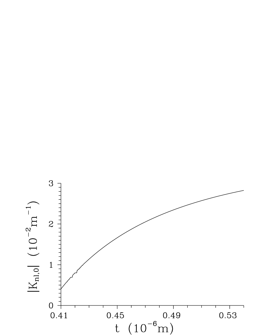
Figure 2: Natural nonlinear phase mismatch $\delta_{nl,0}$ (a) and absolute value of the nonlinear coupling constant $K_{nl,0}$ (b) as they depend on the thickness $t$ of the waveguide are shown in the region of single-mode operation; constant $K_{nl,0}$ is determined for amplitudes that correspond to one pump and one second-subharmonic photon inside the waveguide.

a)      

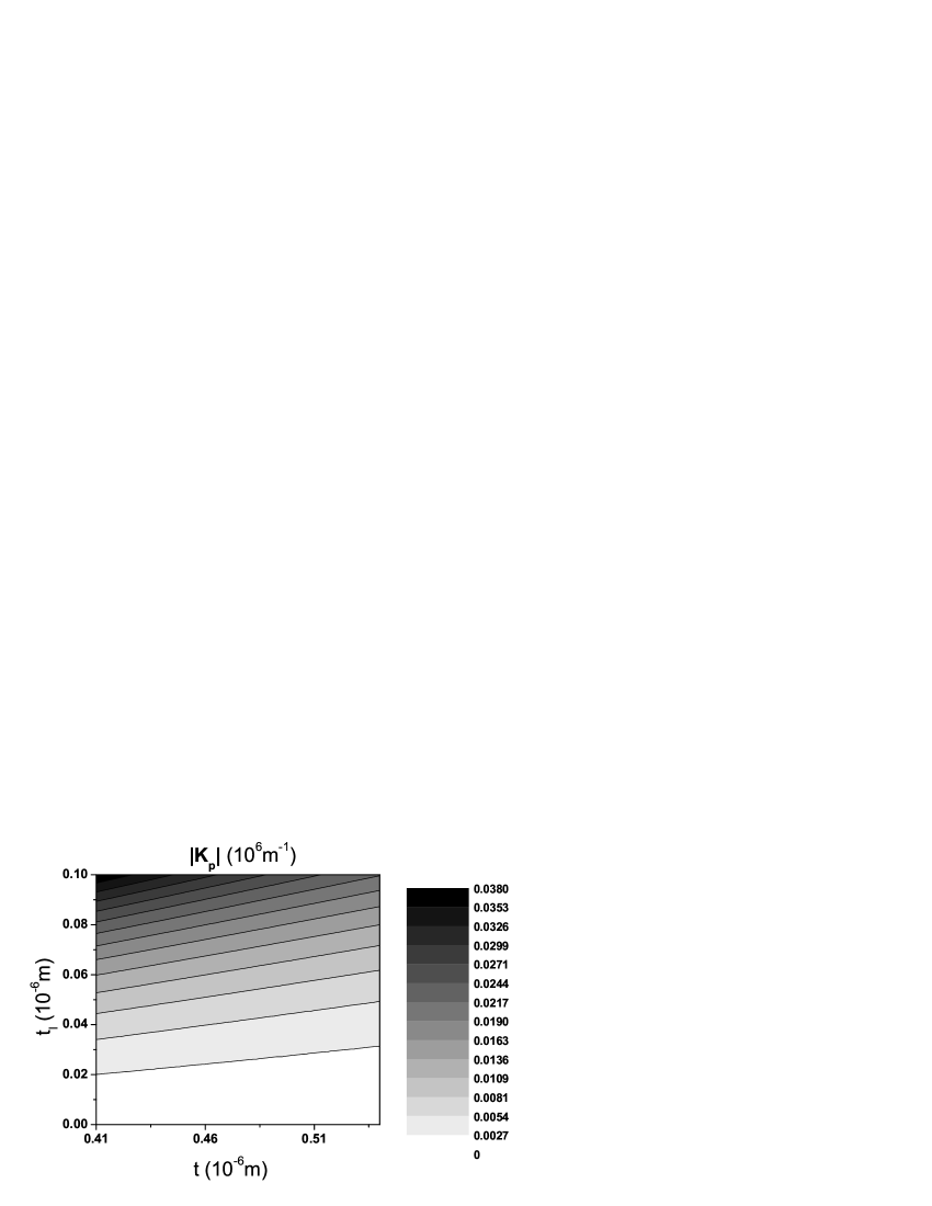
b)      

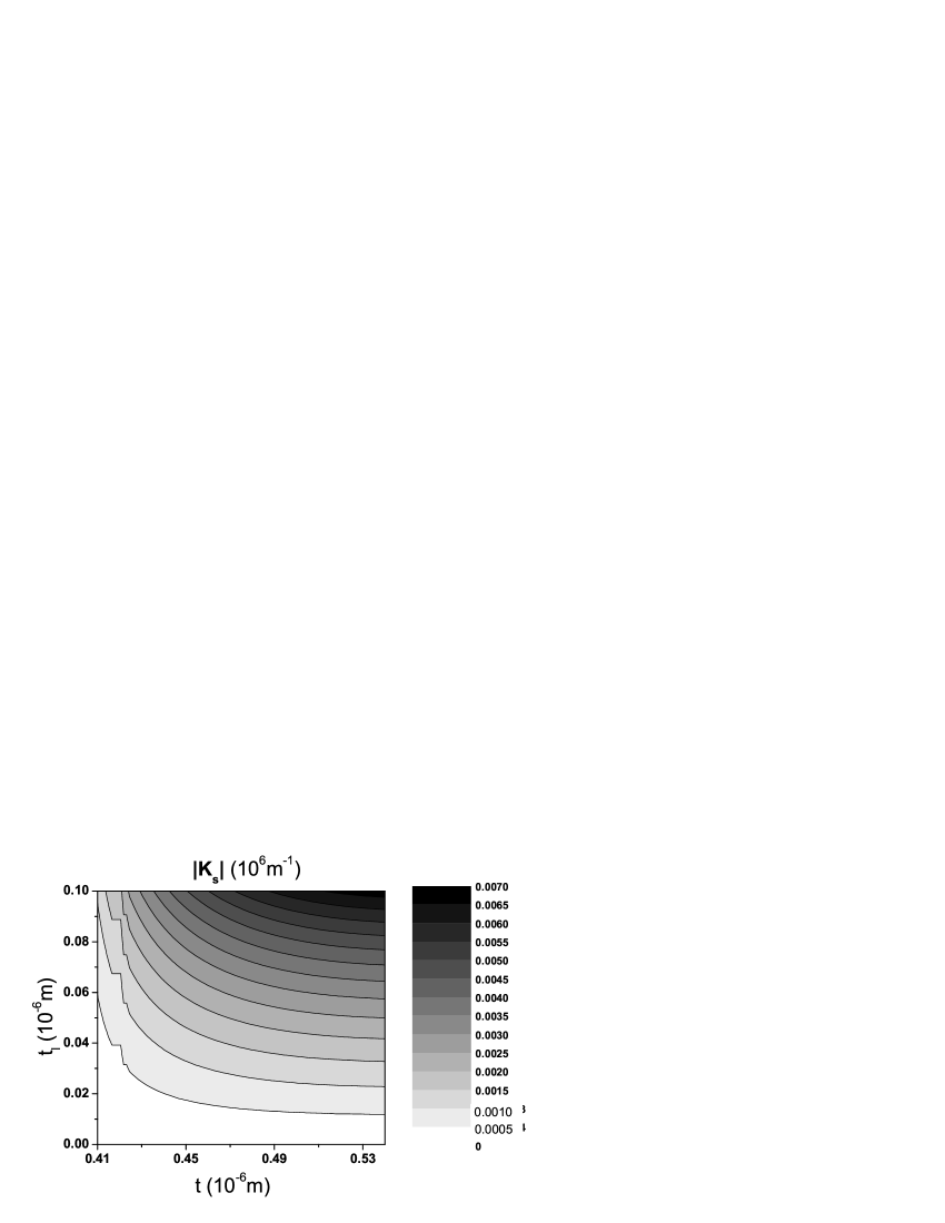
Figure 3: Contour plot of the absolute value of pump-field [second-subharmonic-field] linear coupling constant $K_{p}$ [$K_{s}$] as it depends on thickness $t$ of the waveguide and depth $t_{l}$ of linear corrugation is shown in (a) [(b)] in the region of single-mode operation.

Amplitudes $|A_{a_{b}}|$ of the dimensionless incident strong electric-field amplitudes are determined from the incident power $P_{a_{b}}$ along the relation:

$$|A_{a_{b}}|=\sqrt{\frac{P_{a_{b}}L\beta_{a}}{\hbar\omega_{a}^{2}}},\hskip 8.53581pta=p,s,\hskip 8.53581ptb=F,B.$$ (45)

On the other hand, the power $P_{a_{b}}^{\rm out}$ of an outgoing field is given as follows:

$$P_{a_{b}}^{\rm out} = \frac{\hbar\omega_{a}^{2}}{\beta_{a}L}|A_{a_{b}}|^{2}$$ (46)

$$= \frac{\hbar\omega_{a}^{2}}{\beta_{a}L}N_{a_{b}},\hskip 8.53581pta=p,s,\hskip 8.53581ptb=F,B;$$

$N_{a_{b}}$ denotes the number of photons leaving the waveguide.

New dimensionless parameters are convenient for the discussion of behavior of the waveguide;

$$z^{r}=z/L,$$

$$\Lambda_{l}^{r}=\Lambda_{l}/L,\Lambda_{nl,q}^{r}=\Lambda_{nl,q}/L,$$

$$\beta_{a}^{r}=L\beta_{a},\delta_{a}^{r}=L\delta_{a},K_{a}^{r}=LK_{a},\hskip 8.53581pta=p,s,$$

$$\delta_{nl,q}^{r}=L\delta_{nl,q},K_{nl,q}^{r}=LK_{nl,q}.$$ (47)

Applying these parameters the waveguide extends from $z^{r}=0$ to $z^{r}=1$. The dimensionless parameters enable to understand the behavior of the waveguide as it depends on the length $L$ using the graphs and discussion bellow.

IV.2 Second-subharmonic generation

As a reference for the efficiency of squeezed-light generation we consider the waveguide with periodical poling and assume that it is pumped by the power of 2 W. The nonlinear interaction is perfectly phase matched for the period of poling $\Lambda_{nl}^{r}\approx 3.552\times 10^{-3}$ where we have for the principal squeeze variances $\lambda_{s_{F}}\approx 0.45$ and $\lambda_{p_{F}}\approx 1$ (see Fig. 4). The more distant the value of $\Lambda_{nl}^{r}$ from the above-mentioned optimum value is, the larger the nonlinear phase mismatch and the larger the value of the principal squeeze variance $\lambda_{s_{F}}$.

Figure 4: Principal squeeze variances $\lambda_{s_{F}}$ (solid curve) and $\lambda_{p_{F}}$ (solid curve with $\ast$) as functions of the period $\Lambda_{nl}^{r}$ of poling for second-subharmonic generation; to understand the behavior with respect to the length $L$, the period $\Lambda_{nl}$ should be decomposed as $\Lambda_{nl}^{0}+\Delta\Lambda_{nl}$, then $\delta_{nl,q}^{r}\approx-2\pi q\Delta\Lambda_{nl}^{r}/{\Lambda_{nl}^{0}}^{2}$, $\Lambda_{nl}^{0}=2\pi q/(2\beta_{s}-\beta_{p})$, $\Delta\Lambda_{nl}^{r}=L\Delta\Lambda_{nl}$; $t=5\times 10^{-7}$ m, $K_{p}^{r}=0$, $K_{s}^{r}=0$, $P_{p_{F}}=2$ W, $P_{s_{F}}=1\times 10^{-10}$ W (a negligible seeding to substitute the spontaneous process in the classical equations), $\arg(A_{p_{F}})=0$, $\arg(A_{s_{F}})=0$, $A_{p_{B}}=0$, $A_{s_{B}}=0$; $\Lambda_{nl}^{0}\approx 3.552\times 10^{-6}$ m.

Considering a periodic corrugation in the pump field with such parameters that enhancement of the pump field inside the waveguide occurs, better values of squeezing in the second-subharmonic field can be reached. However, nonzero values of the nonlinear phase mismatch $\delta_{nl,1}$ are important to reach better squeezing because they have to compensate periodic spatial oscillations caused by the corrugation (see Schober2005a ). A perfect phase matching of all the processes occurring in the waveguide can be reached this way [see Eq. (34)].

A typical dependence of the principal squeeze variance $\lambda_{s_{F}}$ as well as the number $N_{s_{F}}$ of photons leaving the waveguide for forward-propagating second-subharmonic field for attainable values of parameters of the corrugation is shown in Fig. 5 assuming a fixed value of the nonlinear phase mismatch $\delta_{nl,1}^{r}$ equal to - 10.82 ($\Lambda_{nl}^{r}=3.53\times 10^{-3}$), i.e. it corresponds roughly to the second local maximum of $\lambda_{s_{F}}$ in the curve in Fig. 4. We can clearly see that an efficient nonlinear interaction occurs in strips that correspond to transmission peaks; the larger the number $m$ of a transmission peak [see Eq. (40)] the weaker the effective nonlinear interaction. The necessity to fulfill also the condition for perfect phase matching given in Eq. (35) is evident. The principal squeeze variance $\lambda_{s_{F}}$ reaches values around 0.2 inside the strips around the first several transmission peaks. The larger the number $m$ of a transmission peak, the greater values of linear coupling constant $K_{p}^{r}$ and linear phase mismatch $\delta_{p}^{r}$ have to be used to reach high levels of squeezing. Up to several forward-propagating photons can be present inside the waveguide (see Fig. 5b) at a given time instant. This means that the power of the outgoing field is of the order of $10^{-8}$ W (energy of one second-subharmonic photon inside the waveguide of thickness $t=5\times 10^{-7}$ m and length $L=1\times 10^{-3}$ m corresponds to the output power of $2.58\times 10^{-8}$ W). Only the first and the second transmission peaks can give reasonable values of the power of the outgoing field.

a)      

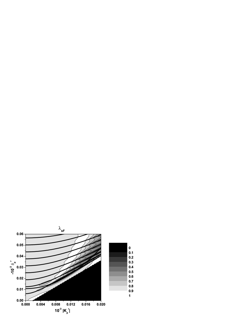
b)      

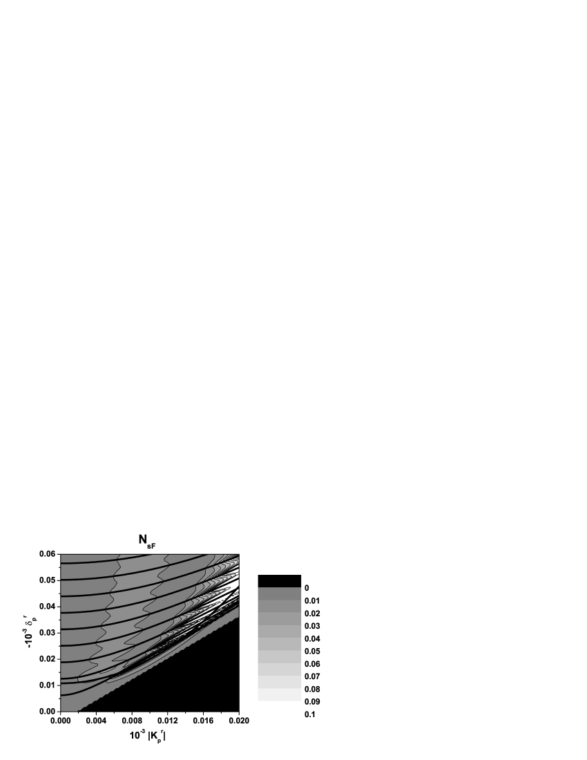
Figure 5: Contour plots of principal squeeze variance $\lambda_{s_{F}}$ (a) and number $N_{s_{F}}$ of photons leaving the waveguide (b) for forward-propagating second-subharmonic field as they depend on parameters $|K_{p}^{r}|$ and $\delta_{p}^{r}$ of the corrugation in the pump field; more-less equidistant curves in the graphs indicate positions of transmission peaks [Eq. (40)], the last curve going up is given by the condition in Eq. (35); $\Lambda_{nl}^{r}=3.53\times 10^{-3}$ ($\delta_{nl,1}^{r}=-10.82$), $\arg(K_{p}^{r})=\pi/2$; values of the other parameters are the same as in Fig. 4. Triangles in lower right corners with formally zero values in both graphs lie in the region with an exponential behavior of classical amplitudes that is not suitable for nonclassical-light generation.

Effect of a periodic corrugation to the enhancement of the nonlinear interaction can be approximately quantified as follows. Because the pump field is strong, its depletion by the nonlinear process can be omitted and its amplitude $A_{p_{F}}(z)$ along the waveguide is given by the formula in Eq. (LABEL:29). In our case, sign + in the condition in Eq. (34) is valid and this means that the nonlinear process exploits efficiently the first term in Eq. (LABEL:29) that is multiplied by the coefficient ${\cal B}_{p_{F}}^{+}$. An effective enhancement of the pump-field amplitude $A_{p_{F}}$ inside the waveguide can be given by the ratio ${\cal B}_{p_{F}}^{+}/A_{p_{F}}(0)$ that we call an enhancement factor ${\cal M}$. The enhancement factor ${\cal M}$ can be expressed as follows provided that the pump field lies in a transmission peak:

$${\cal M}=\frac{2\Delta_{p}+\delta_{p}}{4\Delta_{p}}=\frac{1}{2}+\frac{1}{2}\sqrt{\frac{|K_{p}|^{2}+(m\pi/L)^{2}}{(m\pi/L)2}}.$$ (48)

According to Eq. (48) the greatest value of enhancement factor ${\cal M}$ occurs at the first transmission peak ($m=1$) and the greater the linear coupling constant $K_{p}$ the greater the value of enhancement factor ${\cal M}$. The enhancement factor ${\cal M}$ for the first five transmission peaks is shown in Fig. 6 as a function of the linear coupling constant $K_{p}^{r}$. The greatest enhancement of an electric-field amplitude in the first transmission peak is accompanied by the greatest difference between the maximum and minimum values of electric-field intensities along the waveguide. This poses the question whether other types of distributed feedback resonators (like a quarter wave shifted distributed feedback resonator) giving a more uniform distribution of electric-field intensities along the waveguide Wang1999 can lead even to a better enhancement of the nonlinear process. Modelling of such distributed feedback resonators is, however, beyond the scope of the developed quantum consistent model and so we keep this question open.

Figure 6: Enhancement factor ${\cal M}$ as a function of linear coupling constant $K_{p}^{r}$ for the first five transmission peaks: $m=1$ (solid curve), 2 (solid curve with $\circ$), 3 (solid curve with $\ast$), 4 (solid curve with $\triangle$), and 5 (solid curve with $\diamond$); $t=5\times 10^{-7}$ m.

It is useful to compare the achievable values of the enhancement factor ${\cal M}$ with those typical for cavity geometries. Assuming a symmetric planar cavity with mirrors having intensity reflection $R$, an electric-field amplitude $A^{\rm cav}$ inside a cavity is determined from an incident electric-field amplitude $A^{\rm ini}$ along the formula $A^{\rm cav}=A^{\rm ini}/\sqrt{1-R}$. High quality cavities can have $R=99.9$ % and so the amplitude $A^{\rm cav}$ is enhanced with respect to the amplitude $A^{\rm ini}$ by factor 30, i.e. the enhancement of electric-field amplitudes is considerably greater in this case. On the other hand, the effective nonlinearity increases also due to field confinement in the transverse plane in a waveguide.

Optimum values of waveguide parameters with respect to squeezed-light generation can be determined along the following procedure:

• The greatest possible value of depth $t_{l}$ of a periodic corrugation should be used to maximize the pump-field scattering. This gives the value of linear coupling constant $K_{p}$. From practical point of view, the depth $t_{l}$ of periodic corrugation is limited by technological reasons (also validity of the model would have to be judged for deeper corrugations).

• The value of linear phase mismatch $\delta_{p}^{r}$ should be determined along the relation in Eq. (41) to insure that the pump field is in the first transmission peak. Both signs of the linear phase mismatch $\delta_{p}$ are possible and the corresponding period $\Lambda_{l}$ of linear corrugation is determined according to Eq. (10).

• Solution of Eq. (43) gives an appropriate value of the nonlinear phase mismatch $\delta_{nl,q}$ under the following requirements: sign + in Eq. (43) is used and sign of the determined nonlinear phase mismatch $\delta_{nl,q}$ has to be the same as that of the linear phase mismatch $\delta_{p}$ determined in the previous step.

• Numerical analysis in the surroundings of the analytically-found values of parameters $\delta_{p}$ and $\delta_{nl,\pm 1}$ finally gives the values of waveguide parameters optimum for squeezed-light generation.

This procedure is documented in Fig. 7. The dependence of the optimum value of nonlinear phase mismatch $\delta_{nl,1}^{r}$ on the linear coupling constant $K_{p}^{r}$ is shown in Fig. 7a. The greater the value of linear coupling constant $K_{p}^{r}$ the greater the optimum value of nonlinear phase mismatch $\delta_{nl,q}^{r}$. The corresponding values of the principal squeeze variance $\lambda_{s_{F}}$ are depicted in Fig. 7b. The larger the value of nonlinear phase mismatch $\delta_{nl,1}^{r}$ the better the values of the principal squeeze variance $\lambda_{s_{F}}$. Curves in Fig. 7b also indicate that sign + in Eq. (43) is appropriate and the first transmission peak gives the best values of principal squeeze variance $\lambda_{p_{F}}$. Keeping the incident pump-field power fixed, the depth $t_{l}$ of periodic corrugation limits the achievable values of principal squeeze variance $\lambda_{s_{F}}$.

a)      

b)        

Figure 7: Nonlinear phase mismatch $\delta_{nl,1}^{r}$ as a function of the absolute value $|K_{p}^{r}|$ of linear coupling constant [Eq. (43)] (a) and principal squeeze variance $\lambda_{s_{F}}$ as it depends on the nonlinear phase mismatch $\delta_{nl,1}^{r}$ (b); first (m=1) and second (m=2) transmission peaks as well as signs + and - in Eq. (43) are considered [$m=1+$ (solid curve with $\ast$), $m=1-$ (solid curve with $\diamond$), $m=2+$ (solid curve with $\circ$), and $m=2-$ (solid curve with $\triangle$)]; $\arg(K_{p}^{r})=\pi/2$; values of the other parameters are the same as in Fig. 4.

To see usefulness of the corrugation we compare two configurations: a perfectly quasi-phase matched waveguide and a non-perfectly quasi-phase matched waveguide with a suitable corrugation that compensates for the given phase mismatch. The waveguide with corrugation gives better values of the principal squeeze variance $\lambda_{s_{F}}$ and also considerably greater values of the number $N_{s_{F}}$ of photons leaving the waveguide, as documented in Fig. 8. Also improvement caused by an introduction of corrugation into a non-perfectly quasi-phase-matched waveguide is worth mentioning (see Fig. 8).

a)      

b)      

Figure 8: Principal squeeze variance $\lambda_{s_{F}}$ (a) and number $N_{s_{F}}$ of photons leaving the waveguide for forward-propagating second-subharmonic field as they depend on the incident pump-field power $P_{p_{F}}$ under different conditions: perfect quasi-phase matching ($\delta_{nl,1}^{r}=0$) without corrugation (solid curve), quasi-phase matching with $\Lambda_{nl}^{r}=3.53\times 10^{-3}$ ($\delta_{nl,1}^{r}=-10.82$) without corrugation (solid curve with $\diamond$), and quasi-phase matching with $\Lambda_{nl}^{r}=3.53\times 10^{-3}$ together with a corrugation [its parameters are given by the conditions in Eqs. (43) ($m=1$) and (35)] (solid curve with $\circ$); $\arg(K_{p}^{r})=\pi/2$; values of the other parameters are the same as in Fig. 4.

Benefit of the corrugation to squeezed-light generation can be quantified defining coefficient ${\cal D}$ that gives the ratio (in dB) of the principal squeeze variance $\lambda_{s_{F}}$ reached with a corrugation and the principal squeeze variance $\lambda_{s_{F}}^{\rm ref}$ characterizing a perfectly quasi-phase-matched waveguide without corrugation:

$${\cal D}=-10\log_{10}\left(\frac{\lambda_{s_{F}}}{\lambda_{s_{F}}^{\rm ref}}\right);$$ (49)

$\log_{10}$ stands for decimal logarithm. The value of coefficient ${\cal D}$ determined under the optimum values of parameters of the corrugation as given in Sec. III increases with an increasing incident pump-field power $P_{p_{F}}$ (see Fig. 9). According to curves in Fig. 9 the use of periodic corrugation leads to a significant improvement of squeezing, especially for deeper corrugations and greater incident pump powers.

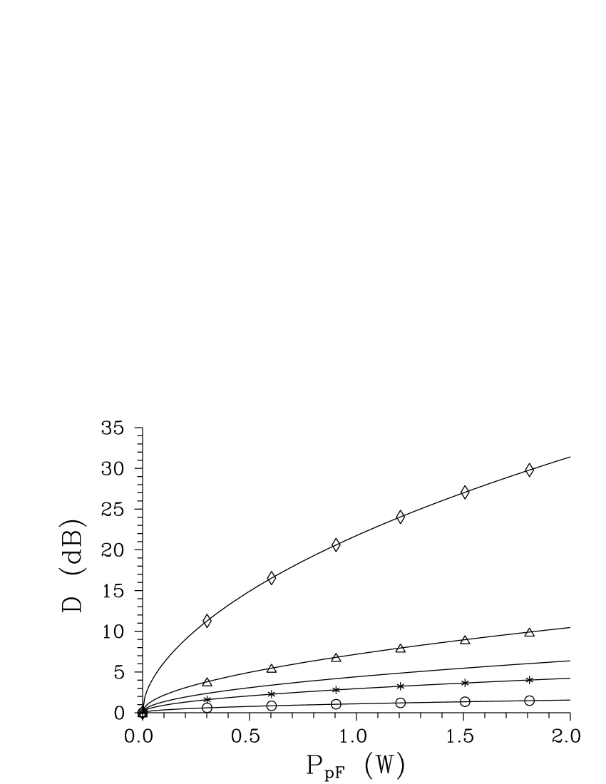
Figure 9: Coefficient ${\cal D}$ giving the improvement of squeezing as it depends on the incident pump power $P_{p_{F}}$ for $|K_{p}^{r}|=5$ (solid curve with $\circ$), $|K_{p}^{r}|=10$ (solid curve with $\ast$), $|K_{p}^{r}|=20$ (solid curve with $\triangle$), and $|K_{p}^{r}|=50$ (solid curve with $\diamond$). Solid curve without symbols is drawn for $\delta_{nl,1}^{r}=-10.82$. Tuning to the first transmission peak ($m=1$) as well as the condition for overall phase matching are assumed; $t=5\times 10^{-7}$ m, $K_{s}^{r}=0$, $\arg(K_{p}^{r})=\pi/2$, $P_{s_{F}}=1\times 10^{-10}$ W, $\arg(A_{s_{F}})=0$, $\arg(A_{p_{F}})=0$, $A_{s_{B}}=A_{p_{B}}=0$.

The role of length $L$ of the waveguide can be addressed using the above-mentioned results as follows. Because the nonlinear phase mismatch $\delta_{nl,1}$ does not depend on the length $L$, the dimensionless nonlinear phase mismatch $\delta_{nl,1}^{r}$ depicted in Fig. 7a is linearly proportional to the length $L$ and, according to curves in Fig. 7b, the larger the value of length $L$ the lower the value of the principal squeeze variance $\lambda_{s_{F}}$. The analysis of conditions in Eqs. (41) and (43) for optimum squeezed-light generation shows that $\delta_{nl,1}\rightarrow|K_{p}|$ and $\delta_{p}\rightarrow 2|K_{p}|$ in the limit of large length $L$. We note that the distance between the curves corresponding to adjacent transmission peaks in contour plots depicted in Fig. 5 behaves as $1/L$.

A periodic corrugation can be alternatively introduced into the second-subharmonic field. The results obtained for principal squeeze variances $\lambda$ and numbers $N$ of photons are comparable to those achieved with a corrugation in the pump field owing to an increase of electric-field amplitudes of the second-subharmonic field inside the waveguide. Suitable conditions are given in Eqs. (38) and (40) in this case.

IV.3 Second-harmonic generation

Second-harmonic generation requires a strong incident second-subharmonic field. As a reference we consider an incident power $P_{s_{F}}$ of the second-subharmonic field to be 2 W and periodical poling giving perfect quasi-phase matching. We then have for the principal squeeze variances $\lambda_{s_{F}}\approx 0.87$ and $\lambda_{p_{F}}\approx 0.99$ ($\Lambda_{nl}^{r}\approx 3.552\times 10^{-3}$).

The nonlinearly interacting fields behave similarly as in the case of second-subharmonic generation. If we introduce a periodic corrugation into the second-subharmonic field and set the nonlinear phase mismatch $\delta_{nl,1}^{r}$ equal to $3.53\times 10^{-3}$, values of the principal squeeze variance $\lambda_{s_{F}}$ approach 0.6 inside the strips in the plane spanned by variables $|K_{s}^{r}|$ and $\delta_{s}^{r}$ where the conditions from Eqs. (38) and (40) are fulfilled (compare Fig. 5). The number $N_{s_{F}}$ of second-subharmonic photons at the output of the waveguide (together with the output power) decreases by an order of magnitude inside these strips compared to the incident power as a consequence of transfer of energy from the strong second-subharmonic field into the pump field (due to an efficient nonlinear interaction) and also transfer of energy into the backward-propagating field (due to scattering) is considerable. Despite this the squeezed second-subharmonic field remains very strong, it contains about $10^{6}$ photons inside the waveguide. The pump field that is only weakly squeezed for perfect quasi-phase matching can reach values of the principal squeeze variance $\lambda_{p_{F}}$ around 0.8 assuming a corrugation with parameters given by Eqs. (38) and (40). The pump field gets a considerable amount of energy from the second-subharmonic field and so typical values of the number $N_{p_{F}}$ of pump photons leaving the waveguide can reach $10^{6}$; i.e. the output power is of the order of $10^{-1}$ W (energy of one pump photon inside the waveguide of thickness $t=5\times 10^{-7}$ m and length $L=1\times 10^{-3}$ m corresponds to the output power of $5.13\times 10^{-8}$ W).

A periodic corrugation can also be put into the pump field and we have qualitatively the same results as if the corrugation is present in the second-subharmonic field. Assuming $\delta_{nl,1}^{r}=-10.82$ as above, values of the principal squeeze variance $\lambda_{s_{F}}$ can reach even 0.3. On the other hand, values of the principal squeeze variance $\lambda_{p_{F}}$ lie above 0.9.

The influence of phases of the interacting optical fields to the nonlinear process is of interest. It can be easily shown that any solution of Eqs. (8) depends only on the phase $\psi=\arg(K_{p})-2\arg(K_{s})$. In our numerical investigations, we did not observe any dependence of numbers $N$ of photons as well as principle squeeze variances $\lambda$ on the phase $\psi$. On the other hand, these quantities depend weakly on phases $\arg(A_{s_{F}})$ and $\arg(A_{p_{F}})$ of the incident fields. However, this dependence is very weak under the conditions where a strongly squeezed light is generated.

At the end, we compare values of squeezing achievable in the considered waveguide with those reached in the commonly used cavity geometries. The best achieved values of squeezing generated in a cavity approach to 10 dB Vahlbruch2007 below the shot-noise level at present, i.e. values of the principal squeeze variance $\lambda_{s_{F}}$ lie slightly above 0.1. The analyzed waveguide does not reach so low values of the principal squeeze variance $\lambda_{s_{F}}$ ($\lambda_{s_{F}}\approx 0.2$) because, as pointed out above, the enhancement of the pump-field amplitude inside the nonlinear medium is considerably lower compared to high quality cavities. On the other hand, the considered waveguide is relatively broad along the $y$ axis ($\Delta y=1\times 10^{-5}$ m) and so narrowing of the waveguide is possible. This would lead to greater values of the effective nonlinearity and subsequently to better values of squeezing. Also longer waveguides can be considered. We believe that the analyzed waveguide with a periodic corrugation has potential to deliver squeezed light with values of parameters comparable to those measured in cavity geometries.

V Conclusions

We have shown that an additional scattering of two nonlinearly interacting optical fields caused by a small periodic corrugation on the surface of the waveguide can lead to an enhancement of the nonlinear process thus resulting in higher generation rates and better values of squeezing. Origin of this enhancement lies in constructive interference of the scattered fields leading to higher values of electric-field amplitudes inside the waveguide. Optimum conditions for this enhancement have been found approximately analytically and confirmed numerically. To observe this effect the natural nonlinear phase mismatch has to be nonzero in order to match with periodic oscillations caused by scattering at the corrugation. The deeper the corrugation and the higher the incident pump power the lower the values of the principal squeeze variances. A periodic corrugation can be designed to match either the pump or the second-subharmonic field, or even both of them.

The obtained results have shown that nonlinear planar waveguides with a periodically corrugated surface represent a promising source of squeezed light for integrated optoelectronics of near future.

Appendix A Modes of an anisotropic waveguide

A mode of the considered waveguide Yeh1988 depicted in Fig. 1 is given as a solution of the wave equation written in Eq. (7). The waveguide is made of LiNbO₃ crystal using the method of proton exchange. The crystallographic $z$ axis coincides with the $x$ axis of the coordinate system (see Fig. 1). Ordinary ($n_{s,o}$) and extraordinary ($n_{s,e}$) indices of refraction of LiNbO₃ valid for the substrate and used in calculations are given as:

$$n_{s,a}^{2} = A_{a}+\frac{B_{a}}{\lambda^{2}-C_{a}}-D_{a}\lambda^{2},\hskip 28.45274pta=o,e,$$ (50)

$$A_{o}=4.91300,B_{o}=0.118717,$$

$$C_{o}=0.045932,D_{o}=0.0278,$$

$$A_{e}=4.57906,B_{e}=0.099318,$$

$$C_{e}=0.042286,D_{e}=0.0224;$$

wavelength $\lambda$ is in $\mu$m. After proton exchange, ordinary ($n_{w,o}$) and extraordinary ($n_{w,e}$) indices of refraction of LiNbO₃ characterizing the waveguide are reached:

$$n_{w,o} = n_{s,o}-\frac{1}{3}\delta n,$$

$$n_{w,e} = n_{s,e}+\delta n,$$

$$(\delta n)^{2} = A_{1}+\frac{B_{1}}{\lambda^{2}-C_{1}}-D_{1}\lambda^{2};$$ (51)

$$A_{1}=0.007596,B_{1}=0.001129,$$

$$C_{1}=0.116926,D_{1}=-0.0003126.$$

We assume that air is present above the waveguide, i.e.:

$$n_{u}=1.$$ (52)

Because only the extraordinary index of refraction of LiNbO₃ increases during proton exchange, only TM waves can be guided. For this reason, instead of solving Eq. (7) for $x$ and $z$ components of the electric-field mode functions ${\bf e}_{a}$, we solve the following equation for the only nonzero $y$ component of the magnetic-field mode functions ${\bf h}_{a}(x)$ (fields are assumed to be homogeneous along the $y$ axis) Snyder1983 :

$$\frac{d^{2}{\bf h}_{a}(x)}{dx^{2}}+\left[-\frac{\bar{\bf\epsilon}_{zz}(x,\omega_{a})}{\bar{\bf\epsilon}_{xx}(x,\omega_{a})}\beta_{a}^{2}+\frac{\bar{\bf\epsilon}_{zz}(x,\omega_{a})\omega_{a}^{2}}{c^{2}}\right]{\bf h}_{a}(x)=0.$$

(53)

The solution of Eq. (53) for $y$ component of the magnetic-field mode function ${\bf h}_{a}(x)$ ($a=p,s$) can be written as:

$$[{\bf h}_{a}(x)]_{y} = -C_{a}\frac{h_{a}}{\tilde{q}_{a}}\exp(-qx),\hskip 5.69054ptx>0;$$ (54)

$$= C_{a}\left[-\frac{h_{a}}{\tilde{q}_{a}}\cos(h_{a}x)+\sin(h_{a}x)\right],\hskip 5.69054pt0<x<-t;$$

$$= -C_{a}\left[\frac{h_{a}}{\tilde{q}_{a}}\cos(h_{a}t)+\sin(h_{a}t)\right]\exp(p_{a}t)$$

$$\mbox{}\times\exp(p_{a}x),\hskip 5.69054ptx<-t;$$

where $C_{a}$ denotes a normalization constant. We have the following expressions for the coefficients $h_{a}$, $q_{a}$, $p_{a}$, $\tilde{p}_{a}$ and $\tilde{q}_{a}$ for the considered orientation of LiNbO₃:

$$h_{a} = \sqrt{\left(\frac{n_{w,o}(\omega_{a})\omega_{a}}{c}\right)^{2}-\left(\frac{n_{w,o}(\omega_{a})}{n_{w,e}(\omega_{a})}\beta_{a}\right)^{2}},$$

$$q_{a} = \sqrt{\beta_{a}^{2}-\left(\frac{n_{u}\omega_{a}}{c}\right)^{2}},$$

$$p_{a} = \sqrt{\left(\frac{n_{s,o}(\omega_{a})}{n_{s,e}(\omega_{a})}\beta_{a}\right)^{2}-\left(\frac{n_{s,o}(\omega_{a})\omega_{a}}{c}\right)^{2}},$$

$$\tilde{p}_{a} = \frac{n_{w,o}^{2}(\omega_{a})}{n_{s,o}^{2}(\omega_{a})}p_{a},$$

$$\tilde{q}_{a} = \frac{n_{w,o}^{2}(\omega_{a})}{n_{u}^{2}}q_{a}.$$ (55)

The solution written in Eq. (54) holds provided that the following dispersion relation giving a propagation constant $\beta_{a}$ as a function of frequency $\omega_{a}$ is fulfilled:

$$\tan(h_{a}t)=\frac{h_{a}(\tilde{p}_{a}+\tilde{q}_{a})}{h_{a}^{2}-\tilde{p}_{a}\tilde{q}_{a}}.$$ (56)

We note that possible solutions of Eq. (56) for $\beta_{a}$ lie in the interval $n_{s,e}(\omega_{a})\omega_{a}/c\leq\beta_{a}\leq n_{w,e}(\omega_{a})\omega_{a}/c$.

Components of the electric-field mode function ${\bf e}_{a}(x)$ can be derived from the magnetic-field mode functions ${\bf h}_{a}(x)$ along the relations:

$$[{\bf e}_{a}(x)]_{x} = \frac{\beta_{a}}{\omega_{a}\epsilon_{0}\bar{\bf\epsilon}_{xx}(x,\omega_{a})}[{\bf h}_{a}(x)]_{y},\mbox{}$$

$$\mbox{}[{\bf e}_{a}(x)]_{y} = 0,$$

$$\mbox{}[{\bf e}_{a}(x)]_{z} = -\frac{i}{\omega_{a}\epsilon_{0}\bar{\bf\epsilon}_{zz}(x,\omega_{a})}\frac{d[{\bf h}_{a}(x)]_{y}}{dx}.$$ (57)

The normalization constants $C_{a}$ occurring in Eqs. (54) are determined from the condition that the mode functions ${\bf e}_{a}(x)$ describe one photon with energy $\hbar\omega_{a}$ inside the waveguide (of length $L$ and thickness $\Delta y$):

$$2\epsilon_{0}\Delta yL\int_{-\infty}^{\infty}dx\left[\bar{\bf\epsilon}_{xx}(x,\omega_{a})\left|[{\bf e}_{a}(x)]_{x}\right|^{2}\right.$$

$$\left.\mbox{}+\bar{\bf\epsilon}_{zz}(x,\omega_{a})\left|[{\bf e}_{a}(x)]_{z}\right|^{2}\right]=\hbar\omega_{a}.$$ (58)

The corrugation on the surface causes periodic changes of values of permittivity ${\bf\epsilon}$ for $x\in(0,-t_{l})$ (see Fig. 1) and we have $\varepsilon_{\pm 1}=i(\bar{\bf\epsilon}-1)/(\pi\bar{\bf\epsilon})$ in this case using Eqs. (2) and (3). If the waveguide is periodically poled ${\bf d}_{\pm 1}=-2i/\pi{\bf d}$ in Eq. (5) and the remaining coefficients may be omitted. Using the electric-field mode functions ${\bf e}_{p}$ and ${\bf e}_{s}$ determined in Eqs. (57), linear ($K_{s}$, $K_{p}$) and nonlinear ($K_{nl,0}$, $K_{nl,1}$) coupling coefficients defined in Eqs. (11) and (LABEL:12) can be rearranged into the form:

$$K_{a} = \frac{i\omega_{a}^{2}}{2\pi c^{2}\beta_{a}}\left[\frac{n_{w,e}^{2}(\omega_{a})-1}{n_{w,e}^{2}(\omega_{a})}\int_{-t_{l}}^{0}dx\,\left|[{\bf e}_{a}(x)]_{x}\right|^{2}\right.$$ (59)

$$\mbox{}\left.+\frac{n_{w,o}^{2}(\omega_{a})-1}{n_{w,o}^{2}(\omega_{a})}\int_{-t_{l}}^{0}dx\,\left|[{\bf e}_{a}(x)]_{z}\right|^{2}\right]$$

$$\mbox{}\times\left[\int_{-\infty}^{\infty}dx\,(\left|[{\bf e}_{a}(x)]_{x}\right|^{2}+\left|[{\bf e}_{a}(x)]_{z}\right|^{2})\right]^{-1},$$

$$\mbox{}\hskip 14.22636pta=p,s,$$

$$K_{nl,0} = \frac{i\omega_{s}^{2}}{2c^{2}\beta_{s}}\int_{-\infty}^{0}dx\,{\bf d}\cdot{\bf e}_{p}(x){\bf e}_{s}^{*}(x){\bf e}_{s}^{*}(x)$$

$$\mbox{}\times\left[\int_{-\infty}^{\infty}dx\,(\left|[{\bf e}_{s}(x)]_{x}\right|^{2}+\left|[{\bf e}_{s}(x)]_{z}\right|^{2})\right]^{-1},$$

$$K_{nl,1} = -\frac{2i}{\pi}K_{nl,0}.$$ (61)

Nonzero coefficients of the nonlinear tensor ${\bf d}$ of LiNbO₃ used in calculations are the following:

$$d_{zzz} = -d_{zyy}=-d_{yyz}=3.1\times 10^{-12}{\rm mV}^{-1},$$

$$d_{xyy} = d_{xzz}=d_{zzx}=d_{yyx}=5.87\times 10^{-12}{\rm mV}^{-1},$$

$$d_{xxx} = 41.05\times 10^{-12}{\rm mV}^{-1}.$$ (62)

- (1) J.A. Armstrong, N. Bloemberger, J. Ducuing, and P.S. Pershan, Phys. Rev. 127, 1918 (1962).
- (2) J. Peřina, Quantum Statistics of Linear and Nonlinear Optical Phenomena (Kluwer, Dordrecht, 1991).
- (3) W. Schleich and A. Wheeler, J. Opt. Soc. Am. B 4, 1715 (1987).
- (4) J. Peřina and J. Bajer, Phys. Rev. A 41, 516 (1990).
- (5) E. Waks, E. Diamanti, B.C. Sanders, S.D. Bartlett, and Y. Yamamoto, Phys. Rev. Lett. 92, 113602 (20024).
- (6) Z.Y. Ou, Phys. Rev. A 49, 2106 (1994).
- (7) R.-D. Li and P. Kumar, Optics Lett. 18, 1961 (1993).
- (8) R.-D. Li and P. Kumar, Phys. Rev. A 49, 2157 (1994).
- (9) D.K. Serkland, M.M. Fejer, R.L. Byer, and Y. Yamamoto, Optics Lett. 20, 1649 (1995).
- (10) D.K. Serkland, P. Kumar, M.A. Arbore, and M.M. Fejer, Optics Lett. 22, 1497 (1997).
- (11) X. Yu, L. Scaccabarozzi, J.S. Harris, Jr., P.S. Kuo, and M.M. Fejer, Optics Express 13, 10742 (2005).
- (12) J. Huang, X.P. Xie, C. Langrock, R.V. Roussev, D.S. Hum, and M.M. Fejer, Optics. Lett. 31 604 (2006).
- (13) A.W. Schober, M. Charbonneau-Lefort, and M.M. Fejer, J. Opt. Soc. Am.B 22, 1699 (2005).
- (14) M.J. Lawrence, R.L. Byer, M.M. Fejer, W. Bowen, P.K. Lam, and H.-A. Bachor, J. Opt. Soc. Am. B 19, 1592 (2002).
- (15) U. Leonhardt, Measuring the quantum state of light (Cambridge Univ. Press, Cambridge, 1997).
- (16) H.-A. Bachor and T.C. Ralph, A Guide to Experiments in Quantum Optics (Wiley-VCH, Weinheim, 2004).
- (17) P. Dong and A.G. Kirk, Phys. Rev. Lett. 93, 133901 (2004).
- (18) J. Peřina Jr. and J. Peřina, Progress in Optics 41, Ed. E. Wolf, (Elsevier Science, Amsterdam, 2000), p. 362.
- (19) J.D. Joannopoulos, R.D. Meade, and J.N. Winn, Photonic Crystals: Molding the Flow of Light (Princeton University Press, Princeton, 1995).
- (20) M. Bertolotti, C.M. Bowden, and C. Sibilia, Nanoscale Linear and Nonlinear Optics, AIP Vol. 560 (AIP, Melville, 2001).
- (21) J.W. Haus, R.Viswanathan, M. Scalora, A.G. Kalocsai, J.D. Cole, and J. Theimer, Phys. Rev. A 57, 2120 (1998).
- (22) D. Pezzetta, C. Sibilia, M. Bertolotti, J.W. Haus, M. Scalora, M.J. Bloemer, and C.M. Bowden, J. Opt. Soc. Am. B 18, 1326 (2001).
- (23) D. Tricca, C. Sibilia, S. Severini, M. Bertolotti, M. Scalora, C.M. Bowden, and K. Sakoda, J. Opt. Soc. Am. B 21, 671 (2004).
- (24) D. Pezzetta, C. Sibilia, M. Bertolotti, R. Ramponi, R. Osellame, M. Marangoni, J.W. Haus, M. Scalora, M.J. Bloemer, and C.M. Bowden, J. Opt. Soc. Am. B 19, 2102 (2002).
- (25) K. Sakoda, J. Opt. Soc. Am. B 19, 2060 (2002).
- (26) M. Scalora, M.J. Bloemer, A.S. Manka, J.P. Dowling, C.M. Bowden, R. Viswanathan, and J.W. Haus, Phys. Rev. A 56, 3166 (1997).
- (27) G. D’Aguanno, M. Centini, M. Scalora, C. Sibilia, Y. Dumeige, P. Vidakovic, J.A. Levenson, M.J. Bloemer, C.M. Bowden, J.W. Haus, and M. Bertolotti, Phys. Rev. E 64, 016609 (2001).
- (28) Y. Dumeige, P. Vidakovic, S. Sauvage, I. Sagnes, J.A. Levenson, C. Sibilia, M. Centini, G. D’Aguanno, and M. Scalora, Appl. Phys. Lett. 78, 3021 (2001).
- (29) Y. Takeno, M. Yukawa, H. Yonezawa, and A. Furusawa, Optics Express 15, 4321 (2007); arXiv:quant-ph/0702139.
- (30) H. Valhbruch, M. Mehmet, N. Lastzka, B. Hage, S. Chelkowski, A. Franzen, S. Goßler, K. Danzmann, and R. Schnabel, arXiv:quant-ph/0706.1434.
- (31) A.W. Snyder and J.D. Love, Optical Waveguide Theory, (Chapman & Hall, London, 1983).
- (32) H.A. Haus, Waves and Fields in Optoelectronics (Prentice Hall, Englewood Cliffs, 1984).
- (33) J. Peřina and J. Peřina Jr., J. Mod. Opt. 43, 1956 (1996).
- (34) N. Korolkova and J. Peřina, Opt. Commun. 137, 263 (1997).
- (35) J. Fiurášek and J. Peřina, Phys. Rev. A 62, 033808 (2000).
- (36) J. Peřina Jr., C. Sibilia, D. Tricca, and M. Bertolotti, Phys. Rev. A 70, 043816 (2004); quant-ph/0405051.
- (37) J. Peřina Jr., C. Sibilia, D. Tricca, and M. Bertolotti, Phys. Rev. A 71, 043813 (2005); quant-ph/0412208.
- (38) W.H. Press, S.A. Teukolsky, W.T. Vetterling, and B.P. Flannery, Numerical Recipes (Cambridge University Press, Cambridge, 1996).
- (39) P. Yeh, Optical Waves in Layered Media (Wiley, New York, 1988).
- (40) A.W. Schober, M.M. Fejer, S. Carrasco, and L. Torner, Optics. Lett. 30, 1983 (2005).
- (41) J.-Y. Wang, M. Cada, and J. Sun, IEEE Photonics Technol. Lett. 11, 24 (1999).