Stochastic processes Lattice theory and statistics (Ising, Potts, etc.) Dynamic critical phenomena

On the occurrence of oscillatory modulations in the power-law behavior of dynamic and kinetic processes in fractals

Abstract

The dynamic and kinetic behavior of processes occurring in fractals with spatial discrete scale invariance (DSI) is considered. Spatial DSI implies the existence of a fundamental scaling ratio ($b_{1}$). We address time-dependent physical processes, which as a consequence of the time evolution develop a characteristic length of the form $\xi\propto t^{1/z}$, where $z$ is the dynamic exponent. So, we conjecture that the interplay between the physical process and the symmetry properties of the fractal leads to the occurrence of time DSI evidenced by soft log-periodic modulations of physical observables, with a fundamental time scaling ratio given by $\tau=b_{1}^{z}$. The conjecture is tested numerically for random walks, and representative systems of broad universality classes in the fields of irreversible and equilibrium critical phenomena.

The understanding of the kinetic and dynamic behavior of the wide variety of phenomena and processes, taking place in disordered and low-dimensional media, is a challenging issue of increasing interdisciplinary interest [1, 2]. The simplest and paradigmatic example is, most likely, the effort devoted to the study of random walks [3]. However, many other examples can also be quoted such as the dynamics of critical systems in condensed matter physics [2, 4]; chemical reactions in catalysts, porous media, nano- and microcavities; annihilation reactions of a wide diversity ranging from magnetic monopoles in the early stages of the Universe to excitons in polymeric matrices [5]; epidemic propagation of diseases and forest fires in far from-equilibrium systems [1, 4, 6]; coarsening dynamics in many systems involving fluids, magnets, and eventually the formation of opinion in social systems [4]; etc. In this letter we address the subtle interplay between time-dependent processes and the symmetry properties of the underlying structure or substrate where the considered process actually takes place. For this purpose, fractal media that exhibit discrete scale invariance (DSI) [7] are considered. DSI is a weak kind of scale invariance such that an observable $O(x)$, obeys the scaling law

$$O(x)=\mu(b)O(bx),$$ (1)

under the change $x\rightarrow bx$. Here $b$ is no longer an arbitrary real number, as in the case of continuous scale invariance, but it can only take specific discrete values of the form $b_{n}=(b_{1})^{n}$, where $b_{1}$ is a fundamental scaling ratio. If an observable $O(x)$ satisfies equation (1) for an arbitrary $b$, it necessary has to obey a power law of the type $O(x)=Cx^{\alpha}$, where $\alpha$ is an exponent. But in the case of DSI, the solution of equation (1) yields

$$O(x)=x^{\alpha}F\left(\frac{\log(x)}{\log(b_{1})}\right),$$ (2)

where $F$ is a periodic function of period one. The detection of soft oscillations in spatial domain [7] is a signature of spatial DSI. Let us consider physical processes that develop a time-dependent characteristic length $\xi(t)$ that increases monotonically, and analyze the behavior of kinetic or dynamic observables, $O(t)$, which characterize these physical processes. If a biunivocal $t=f(\xi)$ relationship holds, we conjecture $\tilde{O}(\xi)=O(t(\xi))$ to obey spatial DSI of the form

$$\tilde{O}(\xi)=\mu(b_{1}^{n})\tilde{O}(b_{1}^{n}\xi).$$ (3)

Now, if we assume that $\xi\propto t^{1/z}$, where $z$ is a dynamic exponent, it is straightforward to show that $O(t)$ has to obey time DSI. In fact, by using equation (2) for $\tilde{O}(\xi)$ and replacing $\xi$ by its explicit time dependence, one has

$$O(t)=Ct^{\alpha/z}F\left(\phi+\frac{\log(t)}{\log(b_{1}^{z})}\right),$$ (4)

where $C$ and $\phi$ are constants. So, if our conjecture given by equation (3) is correct, we would expect to obtain a logarithmic periodic modulation of time observables characterized by a time-scaling ratio $\tau$ given by

$$\tau=b_{1}^{z}.$$ (5)

A relationship between spatial and time DSI was implicitly suggested in connection with the behaviour of earthquakes on a pre-existing hierarchical fault structure [8] and by ourselves in order to account for the dynamic behaviour of a magnet on a fractal substrate [9]. This relationship has also been established in the mathematical literature for the case of a random walk on Sierpinski graphs [10]. In this letter we propose the conjecture given by equation(3) to obtain an explicit relationship between spatial and time DSI according to equation(5). Furthermore, we test our conjecture for three paradigmatic cases in detail, namely i) the behavior of a single random walk and the diffusion-controlled reaction among random walkers [3, 5], ii) the contact process as an archetype of an epidemic process exhibiting irreversible critical behavior [4, 6, 11], and iii) the Ising model that represents a broad universality of reversible (equilibrium) critical phenomena [12].

While equations (4) and (5) are expected to hold for processes occurring in all substrate exhibiting spatial DSI, for the sake of simplicity in this paper we have simulated physical processes on Sierpinski Carpets (SC), which have both infinite and finite ramification orders (IR and FR, respectively), and fractal dimensions within the interval $1.631\leq d_{F}\leq 1.975$. In order to build up a generic SC (SCIR(b,c) or SCFR(b,c)), a square in $d=2-$dimensions is segmented into b^d subsquares and $c$ of them are then removed, and this segmentation process is iterated on the remaining subsquares a number $k$ of segmentation steps. DSI may become evident by measuring some topological property of the fractal, such as the average number of sites belonging to the fractal as a function of the distance to the origin [13], e.g. see figure 1.

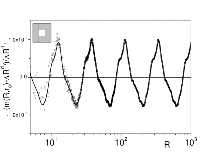
Figure 1: Plot of the number of particles of the fractal located within a distance $R$ from the origin $r_{o}$ $(m(R,r_{o}))$, as a function of $R$. Notice that the vertical axis has been normalized by using the results of the standard power-law fit with an exponent given by the fractal dimension $d_{F}=ln(8)/ln(3)$. For the oscillation, the fit (shown by a continuous line) yields a frequency given by $\omega=2\pi/log(3)$, and involves up to the $5^{th}$ harmonic. The generating cell of the SCIR(9,8) is shown in the top-left corner.

Relevant kinetic observables of random walks are the average number of distinct sites visited after $N$ steps ($S_{N}$) and the mean square displacement from the origin ($R^{2}$), given by

$$S_{N}(t)\propto t^{d_{s}/2},\hskip 14.22636pt{\rm and}\hskip 14.22636ptR^{2}(t)\propto t^{\nu},$$ (6)

respectively [3, 5]. Here we have taken $N\propto t$, while $d_{s}$ is the spectral dimension and $\nu$ is the random walk exponent. For homogeneous media in dimensions $d\geq 2$ one has $d_{s}=2$ and $\nu=1$ leading to classical (standard) diffusion. However, for $d<2$ one has $d_{s}<2$, and the diffusion is anomalous, as diffusion controlled annihilation reactions (such as e.g. $A+A\rightarrow 0$) that no longer obey the classical textbook equation for a second-order reaction, but instead are described by the following anomalous rate equation [5]

$$\frac{d\rho(t)}{dt}=-k_{o}\rho(t)^{X},\rho\rightarrow 0,$$ (7)

where $\rho$ is the density of reacting walkers, $k_{o}$ is the rate constant, and the anomalous reaction order is given by $X=1+2/d_{s}$ [5]. Figures 2(a), (b), and (c) show log-log plots of $S_{N}$, $R^{2}$ and $\rho$ versus $t$ (notice that after a simple integration, equation (7) yields $\rho\propto t^{-d_{s}/2}$), respectively. Results are averaged over $n_{s}$ different configurations.

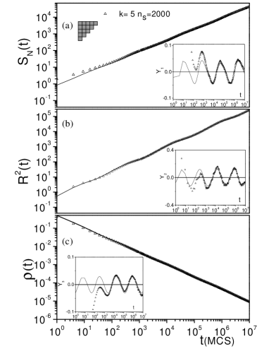
Figure 2: Log-log plot of (a) $S_{N}(t)$, (b) $R^{2}(t)$, and (c) $\rho(t)$ versus $t$, respectively. Results obtained for random walks on the SCFR(5,10) shown in (a). Each of the insets shows, on a linear-log scale, the oscillatory modulation of the corresponding main panel, after previous subtraction and subsequent normalization by the fitted power law. These quantities are denoted by $Y_{m},m=1,2$ and $3$, as taken form the upper to the lower panel, respectively.

The soft oscillatory modulations of the power-law behavior of these observables become more evident after a proper normalization, as shown in the insets of figure 2. Table I summarizes the results obtained by fitting the data with equation (4) up to the $2^{nd}$ harmonic. An excellent agreement (within error bars) between the relevant parameters is obtained: the exponent $d_{s}$, evaluated for a single walk, agrees with the result corresponding to the annihilation reaction; the period of the oscillation is independent of the observable as is the exponent $z$ obtained by applying equation (5). Furthermore, by comparing equations (4) and (6), and taking $R^{2}(t)\propto\xi(t)^{2}$, it follows that $z=2/\nu$, so that the evaluation of $R^{2}(t)$ provides an independent test for the conjectured relationship given by equation (5), (see the $5^{th}$ column of Table I).

Table 1: Results obtained for random walks by fitting the data shown in figure 2 by means of equation (4). The dynamic exponents are obtained by using equation (5) with $b_{1}=5$. More details in the text.

Observable	Exponent	log($\tau)$	$z$	$2/\nu$
$S_{N}(t)$	$d_{s}$ = 1.342(4)	1.785(15)	2.55(2)	—
$\rho(t)$	$d_{s}$ = 1.350(8)	1.72(3)	2.46(4)	—
$R^{2}(t)$	$\nu$ = 0.809(3)	1.75(4)	2.50(6)	2.47(1)

The contact process (CP) [4, 6, 11], is a model for the spreading of an epidemic. It is a one-component non-equilibrium lattice model with spontaneous annihilation and autocatalytic creation of particles. In the CP each site is either vacant or occupied by a single particle. Particles are annihilated at a rate $p$, independent of the states of other sites, and vacancies become occupied at a rate $M/Z$, where $M$ is the number of occupied nearest-neighboring (NN) sites, and $Z$ is the total number of NN sites. The vacuum state of the CP is absorbing and it is reached for $p$ exceeding a critical threshold ( $p\geq p_{c}$). For $p<p_{c}$ the state is fluctuating with an stationary propagation of the activity. So, just at $p_{c}$ one has a second-order irreversible phase transition (IPT). IPT s are often characterized by means of dynamic (epidemic) measurements that allow avoiding undesired finite-size effects [4, 11]. Epidemic measurements are started with a configuration very close to the absorbing state, e.g. the vacuum state with a single particle in the center of the sample for the case of the CP [11]. Subsequently, one measures the average number of particles ($N(t)$) at time $t$, the probability that the system has not entered into the absorbing state ($P(t)$) at time $t$, and the average mean-square distance of spreading ($R^{2}(t)$). In order to obtain appropriate statistic one has to perform many epidemic runs (typically we performed $N_{e}\approx 4\times 10^{4}$ different runs). From the scaling Ansatz of IPT s it follows that, at criticality, the quantities defined above obey, in nonfractal $d-$dimensional spaces, power-law behaviors of the form

$$N(t)\propto t^{\eta},(a)~{}~{}P(t)\propto t^{-\delta},(b)~{}~{}{\rm and}~{}~{}R^{2}(t)\propto t^{z_{e}},(c)$$ (8)

where $\eta$, $\delta$, and $z_{e}$ are the critical exponents. (Notice that, for the sake of clarity, we have used $\nu$ in equation (6) and $z_{e}$ (equation (8(c)) for the exponent of the mean square displacement of the randon walk and the epidemics, respectively.) Figures 3 (a) and (b) show that log-log plots of $N(t)$ and $R^{2}(t)$ versus $t$ exhibit soft log-periodic oscillations modulating the power-law behavior given by equations (8)(a) and (c), respectively. By fitting $N(t)$ with a modulated power law of the type given by equation (4), we can easily identify the critical threshold and decouple the oscillations, as shown in the inset of figure 3(a). Also, for $R^{2}(t)$, with the aid of equation (8)(c) we obtained $z_{e}$ as listed in Table II. As in the case of the random walk, one has that $z=2/z_{e}$, so that the epidemic study allows us to perform independent measurements of the dynamic exponent, see Table III. By considering the error bars, all results corresponding to the CP, which are summarized in Table II, show excellent agreement: the period is independent of the observable, as are the values of $z$, and the independent measurements of $z$ are consistent.

Table 2: Results obtained by performing epidemics in the fractals listed in the first column. The logarithmic period, and the dynamic exponents obtained by using equation (5), for the different observables, are listed in subsequent columns.

$SCIR$	$log(\tau)_{N}$	$z$	$log(\tau)_{P}$	$z$	$log(\tau)_{R^{2}}$	$z$	$2/z_{e}$
(3,1)	0.882(9)	1.85(2)	—	—	0.87(2)	1.83(4)	1.91(1)
(4,4)	1.122(4)	1.863(7)	1.18(2)	1.96(3)	1.12(2)	1.86(4)	1.867(5)
(6,16)	1.415(16)	1.82(2)	1.41(2)	1.81(2)	1.42(2)	1.83(2)	1.835(5)

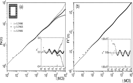
Figure 3: Data corresponding to the CP. (a) Log-log plots of the number of active sites versus time obtained for different values of $p$. In the left-top corner we show the generating cell. (b) Log-log plots of $R^{2}$ versus time obtained at criticality. The insets show the modulating function.

The Ising model is a lattice system where each site $i$ is occupied by a two-state spin variable $\sigma_{i}=\pm 1$[12]. In the absence of external magnetic fields, the Hamiltonian ($H$) is given by $H=-J\sum_{i,i^{\prime}=1}^{N}\sigma_{i}\sigma_{i^{\prime}}$, where $J>0$ is the coupling constant and the summation runs over nearest neighbor sites. In $d>1$ dimensions the Ising model exhibit a continuous phase transition between a ferromagnetic and a paramagnetic phase, which has become the archetypical example for the study of critical phenomena. By starting from a fully ordered configuration with magnetization $M=1$, corresponding to the ground state at $T=0$, after quenching to the critical point one observes a relaxation of the form $M(t)\propto t^{-\beta/\nu z}$, where $\beta$ and $\nu$ are the order parameter and correlation length critical exponents, respectively. We have shown that the relaxation of $M(t)$ exhibits clear evidence of a log-periodic modulation, in the case of the SCIR(4,4) [14] and SCIR(3,1) [9]. We now assume that the observed behavior can be understood in terms of time DSI, allowing us to evaluate $z$. Furthermore, we have performed additional simulations for different fractals, which are summarized in Table III.

Table 3: Critical exponent $\frac{\beta}{\nu z}$, oscillation logarithmic period and dynamic exponent $z$ for the Ising model on several Sierpinski Carpets.

SC	$\frac{\beta}{\nu z}$	$log(\tau)$	$z$
SCIR(5,1)	0.0508(4)	1.61(4)	2.30(6)
SCIR(3,1)	0.0341(1)	1.28(3)	2.69(6)
SCIR(4,4)	0.0110(1)	2.16(1)	3.59(1)
SCIR(5,9)	0.00214(5)	3.47(2)	4.97(3)

Summing up, we have well established a relationship between discrete scaling symmetry invariance, as it is present in fractal structures, and a corresponding symmetry in the time domain for the kinetic and dynamic evolution of different physical systems defined in such structures. We conjecture that the relationship can be obtained by making time observables satisfy spatial DSI symmetry, when they are expresed in terms of the growing length, which characterizes the time evolution. We have also shown that our conjecture implies the presence of time logarithmic oscillations of period $\tau$, linked to the fundamental scaling ratio of the fractal ($b_{1}$) and the dynamical exponent ($z$) (equation (5)). For the sake of simplicity, we have tested numerically our conjecture for relevant archetypical cases on SC substrates. However, our arguments are valid for any fractal exhibiting spatial DSI.

Acknowledgments: This work is supported financially by CONICET, UNLP, and ANPCyT (Argentina). GF acknowledge the ICTP for working facilities.

References

- [1] A. Scott (Ed.), Encyclopedia of Nonlinear Science, Routledge, New York, (2005).
- [2] K. Lindenberg et al (Eds.) J. Phys. Cond. Matt. 19 (2007), special issue containing around 50 papers reporting the state of the art in this topic.
- [3] D. Ben Avraham and S. Havlin, Diffusion and Reactions in Fractals and Disordered Media, Cambridge Universiy Press, Cambridge (2000).
- [4] H. Hinrichsen, Adv.Phys. 49, 815 (2000) and Physica A, 369, 1 (2006).
- [5] R. Kopelman, Science 241, 1620 (1988), L. W. Anacker and R. Kopelman. Phys. Rev. Lett. 58, 289 (1987).
- [6] T. M. Liggett, in Interacting Particle Systems, Spinger, New York, (1985).
- [7] D. Sornette, Phys. Rep. 297, 239 (1998), and references therein.
- [8] Y. Huang, H. Saleur, C.Sammis and D. Sornette, Europhys. Lett. 41, 43 (1998).
- [9] M. Bab, G. Fabricius, E. V. Albano. Phys. Rev. E, 71, 036139 (2005).
- [10] E. Teufl. Combin. Probab. Comput. 12, 203 (2003), and B. Krön, E. Teufl. Trans. Amer. Math. Soc. 356, 393 (2004).
- [11] I. Jensen. Phys. Rev. Lett. 70, 1465 (1993).
- [12] B. M. McCoy and T. T. Wu, “The two dimensional Ising model”. Harvard University Press, Cambridge, MA. (1973); E. Ising, Z. Phys. 31, 253 (1925).
- [13] Y. Huang, G. Ouillon, H. Saleur and D. Sornette, Phys. Rev. E. 55, 6433 (1997).
- [14] M. Bab, G. Fabricius, E. V. Albano. Phys. Rev. E,74, 041123 (2006).