Extremality conditions for isolated and dynamical horizons
Abstract
A maximally rotating Kerr black hole is said to be extremal. In this paper we introduce the corresponding restrictions for isolated and dynamical horizons. These reduce to the standard notions for Kerr but in general do not require the horizon to be either stationary or rotationally symmetric. We consider physical implications and applications of these results. In particular we introduce a parameter which characterizes how close a horizon is to extremality and should be calculable in numerical simulations.
I Introduction
It is well known that there is a limit on the maximum allowed angular momentum for a Kerr black hole. If such a hole has mass then the angular momentum must satisfy . Solutions which saturate this bound are known as extremal while Kerr spacetimes with contain naked singularities rather than black holes. Given this constraint on stationary solutions it is natural to consider whether there is a similar restriction for astrophysical black holes. In contrast to the Kerr holes which sit alone in an otherwise empty universe, real black holes do not exist solely in isolation and can, for example, be surrounded by accretion disks or be components of binary systems.
For this reason, it is interesting to investigate whether extremality conditions can be formulated and applied to interacting black holes. This is of particular interest during black hole collisions. It is widely accepted that following a merger, the final black hole will settle down to one of the known stationary solutions. However, during the highly dynamical merger phase, it is not clear whether the black hole’s angular momentum is bounded. The existence or lack of an extremality condition may help us to understand the physics of black hole mergers, and provide insight into whether binary black holes will necessarily “hang up” in orbit, emitting excess angular momentum prior to forming a common horizon. Similar questions arise for black holes forming from the gravitational collapse of matter.
Away from the Kerr–Newmann family of solutions there are some recent results that either support or cast doubt on the possible existence of such a bound. In support, Dain Dain (2006a, b, c) has shown that for a large class of asymptotically flat, axially symmetric, vacuum black holes where the subscripts indicate that these are the ADM mass and angular momentum as measured at spatial infinity. By contrast Petroff and Ansorg Ansorg and Petroff (2005, 2006); Petroff and Ansorg (2005) have recently generated numerical examples of black holes surrounded by rotating rings of matter for which the Komar mass and angular momentum violate the bound .
Clearly in considering these issues one needs to be careful about how the physical quantities are defined. In particular, in formulating a bound one would like to distinguish between the mass and angular momentum directly associated with the black hole versus any matter or gravitational waves surrounding it. This is, of course, easier said than done. Mass and energy are notoriously ambiguous quantities in general relativity. They are well-defined for entire asymptotically flat spacetimes but in general it is not possible to assign mass and energy to more localized regions of spacetime (see, for example, the discussion in Szabados (2004)). Similar problems arise for angular momentum and away from axi-symmetry it is not at all clear that angular momentum can be described by a single number.
Distinguishing between local and global properties of black holes is one of the main motivations for the recent interest in quasilocal characterizations of horizons, including trapping Hayward (1994, 2004a, 2006a, 2004b), isolated Ashtekar et al. (1999); Ashtekar et al. (2000a, b); Ashtekar et al. (2000c, 2001), and dynamical Ashtekar and Krishnan (2002, 2003) horizons. In this paper we apply the machinery developed in the study of quasilocal horizons to investigate local characterizations of extremality.
We will argue that the ambiguities in defining mass and angular momentum mean that, in general, the usual Kerr extremality bound is not well formulated for quasilocal horizons. Thus we will examine alternative characterizations of extremality and show that they do apply. For isolated horizons these arise from 1) the non-negativity of the surface gravity and 2) the idea that there should be trapped surfaces just inside the horizon. For dynamical horizons only the second these characterizations is applicable since the surface gravity is only meaningful for slowly evolving dynamical horizons (in the sense of Booth and Fairhurst (2004); Kavanagh and Booth (2006); Booth and Fairhurst (2007)).
Both the surface gravity and trapped surface characterizations of extremality give rise to an alternative, local extremality condition. This condition is similar in spirit to the Kerr extremality bound, and involves contributions from both the black hole’s angular momentum and horizon matter fields. However, it can be written locally on the horizon and angular momentum ambiguities are avoided by making use of the square of an “angular momentum density” integrated over the horizon rather than the angular momentum relative to any particular axis. With this definition of extremality, we show that generic dynamical horizons, in the sense of Ashtekar and Galloway (2005), are necessarily sub-extremal. Isolated horizons can obtain extremality (in which case the local geometry must be that of the Kerr horizon Lewandowski and Pawlowski (2003)). We discuss how this local extremality compares to the standard Kerr relation, and argue that in those cases where both are well formulated it may still be possible for a black hole to violate the Kerr bound.
The paper is laid out as follows. We begin in Section II with a discussion of extremality for stationary black holes and recall the three notions of extremality already mentioned: maximum angular momentum, vanishing surface gravity, and coincidence of the inner and outer horizons. The next section shows how these notions may be adapted to isolated horizons, examines conditions under which they are equivalent, and considers situations under which one or more of them might be violated. In Section IV we use this experience to study the equivalent notions for dynamical horizons and show that these horizons are always sub-extremal. Finally, Section V provides a brief summary. An Appendix shows how the various notions apply to the Kerr (anti-)deSitter family of solutions.
II Stationary Black Hole Horizons
Let us begin by reviewing the notion of extremality for stationary, asymptotically flat black hole space-times. In Einstein–Maxwell theory, the uniqueness theorems tell us that the class of such solutions is restricted to the Kerr–Newman space-times. Furthermore, these space-times are characterized by only three quantities; their mass M, angular momentum J and electric charge Q. Black hole solutions exist for all values of , and which satisfy the inequality:
| (1) |
If this inequality is violated the resulting spacetimes are still solutions of the Einstein equations, however they contain a naked singularity in lieu of a black hole. The first notion of extremality arises from Eq. (1). Solutions for which the equality is satisfied, namely
| (2) |
are said to be extremal as they contain the maximum allowed angular momentum/charge for a given mass.
Since the Kerr–Newman solutions are stationary and axi-symmetric, they have both a time-translation Killing vector field and a rotational Killing vector field . The event horizon is a non-expanding null surface whose null normal is
| (3) |
where is interpreted as the angular velocity of the horizon. It is then straightforward to calculate the acceleration of at the horizon:
| (4) |
The quantity is known as the surface gravity. Since is defined in terms of Killing vectors which are appropriately normalized at infinity, there is no ambiguity in its normalization and by direct calculation
| (5) |
The second notion of extremality comes from this surface gravity. It is clear from Eqs. (1) and (5) that the surface gravity is only well-defined for black hole (as opposed to naked singularity) solutions and is necessarily non-negative. Furthermore, for an extremal black hole satisfying (2), the surface gravity vanishes, i.e. . Thus, vanishing surface gravity is often taken as the defining property of an extremal horizon.
Finally, we can understand extremality from the geometric structure of space-time — one of the fundamental properties of a black hole is that it contains trapped surfaces which are defined in the following way. Any spacelike two-surface has two future-pointing null normals, which we will denote and . Then, the expansion of these null vectors is defined as:
| (6) |
where is the metric of the two-surface. On a trapped surface, the expansions of both null vector fields are negative. This is in contrast to a typical (convex) two-surface in flat space which will have one positive and one negative expansion. For asymptotically flat spacetimes, the existence of a trapped surface is sufficient to imply the existence both an event horizon enclosing the surface and a space-time singularity somewhere in its interior Penrose (1965).
For typical charged or rotating black holes, there are two horizons, the event horizon and the inner Cauchy horizon. These are null, foliated by two-dimensional marginally trapped surfaces ( and ), and split the space-time into distinct regions. It is only in the region between the horizons that trapped surfaces exist. If the charge or angular momentum is increased towards the extremal value, the trapped region between the horizons shrinks, until, at extremality, the inner and outer horizons coincide, the trapped region vanishes and only the marginally trapped surfaces of the horizon remain. It is this notion of extremality which is used in Israel’s proof that a non-extremal black hole cannot achieve extremality in a finite time Israel (1986).
Thus, we see that for event horizons in stationary space-times, there are three notions of horizon extremality which all coincide:
- First Characterization:
-
The angular momentum and charge of a black hole are restricted according to Eq. (1). For an extremal black hole, .
- Second Characterization
-
The surface gravity of a black hole must be greater than or equal to zero. The surface gravity vanishes if and only if the horizon is extremal.
- Third Characterization
-
The horizon of the black hole is a marginally trapped surface. For non-extremal black holes, the interior of the black hole must contain trapped surfaces, while for extremal black holes, the inner and outer horizons coincide and there are no trapped surfaces.
In the remainder of this paper, we will argue that the second and third definitions can be extended to isolated and dynamical horizons. Furthermore, we will obtain a horizon relation similar in spirit, though not identical, to the one appearing in the first definition above. We start with isolated horizons.
III Isolated Horizons
Isolated horizons have been introduced to capture the local physics of the horizon of a black hole in equilibrium Ashtekar et al. (1999); Ashtekar et al. (2000a, b); Ashtekar et al. (2001, 2000c). These are null surfaces and so form causal boundaries. However, unlike event horizons, they are defined (quasi-)locally. Specifically, a null surface of topology with (degenerate) metric , derivative , and normal is an isolated horizon if:
-
1.
is non-expanding: ,
-
2.
an energy condition holds at the horizon: is future-directed and causal, and
-
3.
the null vector is scaled such that
(7)
The energy condition is weaker than and implied by any of the standard energy conditions. Together with the first condition and the Raychaudhuri equation it follows both that the intrinsic geometry of is invariant in time: and that there is no flux of matter through the horizon: . The third condition fixes the scaling of up to an overall constant and ensures that the extrinsic geometry is similarly invariant in time.
To make all of this a little more concrete, note that one can always find functions on that are compatible with (so that ) and which have spacelike level surfaces with topology . For such a function, is not only normal to these surfaces of constant but is also null and satisfies . The spacelike metric on the can be written as .
With these additional structures the invariance of the intrinsic geometry can be written as
| (8) |
so that both the expansion and shear of the two-surfaces vanish. Further, the third condition implies that the corresponding expansion and shear in the -direction are also invariant in time
| (9) |
as is the connection
| (10) |
on the normal bundle to the foliation two-surfaces:
| (11) |
Finally, one can use the axioms to prove a zeroth law. For the allowed scalings of the null vectors, the surface gravity , defined in a similar manner to that on the event horizon (4),
| (12) |
is constant on the horizon: Ashtekar et al. (2000b).
On an isolated horizon, the scaling of the null vectors is only fixed up to an overall positive multiplicative constant. Under allowed rescalings and , the connection is invariant while . Thus, while is constant over , its exact value is only fixed up to sign (ie. positive, negative, or zero).
Derivations of these facts can be found in the already cited references or in Ashtekar et al. (2002) which focuses on the geometry of horizons.
III.1 Extremality from , and ?
We begin with the first notion of extremality: the horizon of a Kerr–Newman black hole is extremal if and only if . Let us attempt to extend this to isolated horizons. The prerequisite to this is to obtain a satisfactory definition of each of these quantities and, except for the electric charge, that is where problems arise. Given a two-dimensional cross-section of the horizon, the charge is well-defined by Gauss’ law:
| (13) |
where is the determinant of the two-metric on and is the electromagnetic field tensor. Equivalently, we rewrite where and respectively are orthogonal timelike and spacelike unit normal vectors to . is the flux of the electric field through as observed by a timelike observer with evolution vector . Since the horizon is isolated, this is independent of the cross-section Ashtekar et al. (2000b).
Next, we consider angular momentum. In classical, non-relativistic, physics angular momentum is defined relative to an axis of rotation. For isolated horizons the analogue of an axis of rotation is a rotational vector field. Following Booth and Fairhurst (2004, 2005, 2007) this is given by whose flow foliates the into closed integral curves of parameter length plus two fixed points (the poles of the rotation). A vector field of this type is necessarily divergence-free and the canonical example is a horizon with a rotational Killing vector field so that
| (14) |
The angular momentum relative to a rotational vector field is then Ashtekar et al. (2001, 2000c)
| (15) |
where is the connection of the normal bundle that we have already encountered in Eq. (10), and is the electromagnetic connection. It is immediate that on an isolated horizon this quantity is independent of the choice of cross-section .
This is closely related to other standard measures of angular momentum such as the Brown-York Brown and York (1993) or dynamical horizon Ashtekar and Krishnan (2003) measures. In particular, as is discussed in more detail in Ashtekar et al. (2000b)
| (16) |
is the Weingarten map and is analogous to the standard extrinsic curvature, although tailored to the null surface of the horizon. Then, it is not surprising that the geometric part of the angular momentum (15) agrees with usual extrinsic curvature formula. To see this, consider the case where the isolated horizon is an apparent horizon found in a numerical simulation. In this case, the are each contained in spacelike three-surfaces , is the future directed unit normal to the and is the outward-pointing spacelike unit normal to the . Then, for a divergence-free rotational vector field it is straightforward that the isolated horizon angular momentum can be rewritten as
| (17) |
where is the extrinsic curvature of (with the induced three-metric on ). In stationary blak hole spacetimes, this measure also agrees with the Komar and ADM angular momenta evaluated at infinity.
Thus, given a rotational vector field the angular momentum of the horizon is well-defined. Unfortunately, in the absence of axi-symmetry there is no obvious way to uniquely select a geometrically preferred rotational vector field. Indeed, for highly distorted horizons, it is by no means clear that one should always expect such an “axis of rotation” to exist. For non-axisymmetric horizons it seems unlikely that the angular momentum can be characterized by a single number (though see Dreyer et al. (2003); Schnetter et al. (2006); Hayward (2006b); Cook and Whiting (2007); Korzynski (2007) for alternative viewpoints).
Even if we restrict our attention to axially symmetric horizons, in order to define extremality by Eq. (1) we would still need a definition of horizon mass and here the greatest difficulties arise. While local definitions of angular momentum for a surface are readily available and tend to agree, the issue of a local energy or mass is much more difficult Ashtekar et al. (2000b); Booth and Fairhurst (2005); Szabados (2004). In particular, the rescaling freedom of precludes the identification of a preferred energy associated with evolution along . A common solution to this is to simply define the mass of a horizon with area and angular momentum to be equal to the value it would take in the Kerr space-time. Then by the Christodoulou formula Christodoulou (1970)
| (18) |
where is the areal radius of the horizon. With this mass, it is straightforward to show that is less than . However this is simply a property of the definition and the physical relevance of (18) for highly distorted black holes is, at best, unclear.
Given the difficulties with the definition of mass, it probably makes more sense to rephrase any characterization of type (1) entirely in terms of quantities such as , , and which can be locally measured on the horizon. Then, this bound may be rewritten as
| (19) |
Thus defining , , and as we have above, this is the first possible characterization of extremality, at least for axi-symmetric horizons. There is no general derivation that this bound must hold outside of the Kerr–Newman family. Indeed, the inequality in Eq. (19) can be violated for non-asymptotically flat spacetimes (Appendix A). Similarly, in higher dimensional asymptotically flat space-times the original bound (1) can also be violated Myers and Perry (1986); Emparan and Myers (2003). Despite this, Ansorg and Pfister have demonstrated that (19) holds (with equalilty) for a class of extremal configurations of black holes surrounded by matter rings. Furthermore, they have conjectured that the inequality will hold for stationary, axially and equatorially symmetric black hole–matter ring solutions Ansorg and Pfister (2007).
III.2 Extremality from
The second notion of extremality for Kerr black holes says that the surface gravity is positive for sub-extremal holes and zero for extremal holes. It is never negative. We now consider this characterization for isolated horizons and see that in many ways it is more satisfactory than that considered in the previous section.
The surface gravity for an isolated horizon was given in Eq. (12), where it was noted that a zeroth law holds so that everywhere on for some (fixed) . The scaling of the null vectors is only fixed up to a positive multiplicative constant so rescalings of the form , are allowed. For such rescalings and so the formalism only allows us to say whether an isolated horizon has a surface gravity that is positive, negative, or zero. This is sufficient for our purposes; an isolated horizon is sub-extremal if and only if , extremal if , and super-extremal if .
Such a definition is more than just nomenclature. For there is a local uniqueness theorem for isolated horizons; the intrinsic geometry of an extremal isolated horizon must be identical to that of the Kerr–Newmann horizon with the same area, charge and angular momentum Lewandowski and Pawlowski (2003). Further, sub-extremal horizons must obey bounds on their electric charge and the angular momentum one-form . To see this, note that the the evolution of is given by Ashtekar et al. (2000b); Booth and Fairhurst (2007):
| (20) |
where is the two-curvature of the cross-sections of the horizon, is the spacelike two-metric compatible covariant derivative and is the energy-momentum tensor.
The standard definition of an isolated horizon doesn’t restrict the sign of the inward expansion . However, since we are interested only in black hole horizons333The defining conditions for isolated horizons are intended to be necessary conditions that a null surface should meet in order to be considered as the boundary of a non-interacting black hole region. However, they are not sufficient to distinguish black hole horizons from white hole or cosmological horizons. Furthermore, there are examples of isolated horizons which either do not correspond to black holes (in Pawlowski et al. (2004) there are no trapped surfaces) or their black hole status is unclear (in Fairhurst and Krishnan (2001) it is not known whether the “black holes” all contain trapped surfaces)., it is reasonable to impose the extra requirement that there be trapped surfaces “just inside” the horizon. Thus, by continuity we restrict our attention to horizons with .
Now, consider equation (III.2) evaluated on a sub-extremal isolated horizon. On the left-hand side, the first term will vanish since the geometry is time independent. The second term is necessarily non-positive: by assumption surface gravity is non-negative, and we have restricted to black hole horizons where . Finally, although the itself can vary in sign, we know that since the cross-sections of the horizon have topology , .
Thus, integrating (III.2) over any gives
| (21) |
(the integral of the exact derivative vanishes). This gives an alternative characterization of extremality for isolated horizons: vanishes if and only if and is positive if and only if . This expression provides a local extremality condition for isolated horizons expressed in terms of the horizon angular momentum (encoded in the one-form ) and matter fields. As such, it is similar in spirit to the standard Kerr bound. However, this condition is applicable to all isolated horizons, and does not require either axi-symmetry or asymptotic flatness.
The exact interpretation of the matter term depends on the matter present at the horizon, but for electromagnetism it is related to the electric and magnetic charge of the hole:
| (22) |
The first term is the square of the electric flux density, while the second is the square of the corresponding magnetic flux — the integral of is the magnetic charge contained by .
The second term of (21) is associated with angular momentum. It side-steps the problems of defining an axis of rotation by working with the square of the angular momentum density integrated over the horizon as a measure of the total angular momentum. To gain some insight into this quantity, consider an axi-symmetric horizon. On such a horizon, the angular momentum can be decomposed into its multipole moments Ashtekar et al. (2004). Based on this decomposition, can be interpreted as the dipole angular momentum of the horizon. Then the quantity appearing in our extremality condition (21) can, at least intuitively, be thought of as the sum of the squares of all the angular momentum multipoles of the horizon.
These associations can be made concrete by calculating for the known black hole solutions. First for Reissner–Nordström space-times (where vanishes) it is straightforward to show that
| (23) |
where is the charge and is the areal radius of the horizon. Thus corresponds to the extremality condition while implies that .
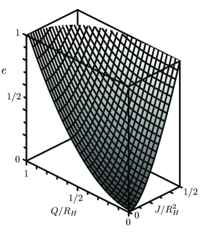
Moving on to the Kerr–Newman solutions the functional form of becomes considerably more complicated and so instead of stating it explicitly, we plot it in Fig. 1 as a function of the angular momentum and electric charge. Recall from Eq. (19) that the standard extremality condition for Kerr–Newman solutions can be written as . Then from the figure, we see that for these extremal solutions while for non-extremal solutions . Therefore, the local extremality quantity behaves as expected for stationary, asymptotically flat black holes.
III.3 Trapped surfaces
Finally we consider the third characterization of extremality: a horizon is sub-extremal if there are trapped surfaces “just inside” the horizon and extremal (or super-extremal) if there are no such surfaces. For this notion we need to understand how the properties of a surface change under infinitesimal deformations. Continuing to assume that on the horizon (and so by continuity remains negative for sufficiently small deformations), we are then interested in cases where there exists an inward deformation so that also becomes negative. The equations governing such deformations have been derived and rederived many times and in many ways over the years Newman (1987); Gourgoulhon (2005); Gourgoulhon and Jaramillo (2006); Korzynski (2006); Eardley (1998); Hayward (1994); Booth and Fairhurst (2007). Here we follow Booth and Fairhurst (2007).
There, it is shown that given a spacelike two-surface and a transverse deformation vector field ,
| (24) |
where and are the components of deformation vector relative to the null normals so that . Furthermore,
| (25) |
(the Raychaudhuri equation with ) and
| (26) |
are the variations of under the deformations generated by the null vectors. One way of calculating these deformations is to construct a coordinate system on the manifold for which is parameterized by two-coordinates (say ) and is a level surface with respect to the other two. The deforming vector (be it , or ) should be a tangent vector field to one of these other coordinates. For such a construction, quantities such as can be defined on level surfaces of the non- coordinates in a neighbourhood of . Then the s are Lie derivatives. In fact we have already seen an example of this type of construction in this paper; equation (III.2) could equally well be written as . Indeed, Eq. (26) can be obtained from (III.2) by simply switching and and noting that .
Inward deformation vector fields will necessarily take the form where . For simplicity, we can rescale the null vectors such that . Let us denote these rescaled vectors as , . Then
| (27) |
since on an isolated horizon regardless of the scaling on the null vectors (note that this result is independent of Eq. (7) ). Thus, slices of the horizon may be deformed inwards into fully trapped surfaces if and only if there is a scaling of the null vectors such that .
By this measure we characterize an isolated horizon as sub-extremal if there exists a scaling of the null vectors such that , extremal if there exists a scaling such that , and super-extremal if there exists a scaling such that . It is important to keep in mind that each of these conditions must hold everywhere on and that it will usually be non-trivial to find the correct scaling needed for the classification.
The Kerr solutions themselves provide an example of these difficulties. For rapidly rotating Kerr black holes with the usual (Killing vector) scaling of the null vectors, varies in sign over . However, this does not indicate that these horizons lie outside the classification system. Instead it suggests that a different scaling of the null vectors is needed. Such a rescaling is considered explicitly in Appendix C of Booth and Fairhurst (2007), however here we generalize that calculation to prove a more general result: for axi-symmetric isolated horizons with the surface gravity and trapped surface classifications of extremality are equivalent. That is
| Sub-extremal: | ||||
| Extremal: | and | |||
| Super-extremal: |
where and are appropriate rescalings of the null vectors.
We prove this result by explicitly constructing these rescalings. To this end we first note the following key fact: On a topologically spherical two-surface embedded in spacetime there is always a scaling of the null vectors so that the angular momentum one-form is divergence-free: (this result ultimately follows from the Hodge decomposition theorem Ashtekar et al. (2002)). The scaling is unique up to the usual multiplicative constant. Thus, taking such a pair of vectors (,) as a reference, we can write any other scaling of the null vectors as
| (28) |
for some scalar function over . Then we can define the inverse scaling
| (29) |
and using equations (III.2) and (26) it is straightforward to see that on an isolated horizon:
| (30) |
For an axisymmetric horizon the dual requirements that respect the symmetry and that not diverge at the poles of rotation imply that must be parallel to the rotation vector. Then the last term of (30) vanishes and we find that
| (31) |
The result is established. As a corollary, the value of the extremality parameter is the same evaluated for either the constant surface gravity scaling of the null vectors or the corresponding inverse scaling.
In more general situations, deciding on the classification of a horizon will amount to studying the properties of a second order elliptic partial differential operator. In particular, again taking as reference scalings we have
| (32) |
where
| (33) |
and we wish to find functions for which (32) is everywhere negative (or zero or positive).
We will not investigate this equation in detail in this paper but instead content ourselves with proving that, in general, the classification is well defined. That is, given a scaling of the null vectors so that is everywhere negative, it is impossible to rescale the vectors so that the horizon becomes extremal or super-extremal. Physically this is equivalent to saying that there cannot be both trapped and untrapped surfaces “just inside” the horizon.
To see this, we reuse Eq. (32) though this time take as any scaling of the null vectors and as some rescaling by . Let us assume for a moment that is analytic. Then if it is not constant it must have maximum and a minimum. At each of these vanishes while is respectively greater or less than zero. Thus at : while at : and it is clear that if then will have a mixed sign. Similarly if is everywhere positive (or negative) then it cannot be rescaled to be everywhere negative (or positive). These results extend to non-analytic rescalings with the help of the maximum principle (see for example Booth and Fairhurst (2007)) and so it is clear that rescalings cannot change the classification of a horizon.
Finally, note that we have not eliminated the possibility that some isolated horizons might exist which do not fall into any of the three categories. That is, there may be horizons for which no rescaling will cause to either vanish or be positive/negative everywhere. A source of potential examples are the distorted horizons discussed in Fairhurst and Krishnan (2001).
III.4 A bound on angular momentum
With these two notions of extremality established let us now return to the first: is there a maximum angular momentum for rotationally symmetric isolated horizons? In answer to this question we now show that the allowed angular momentum is bound by the intrinsic geometry of the horizon and in particular for a large class of horizons, that bound is exactly the local version of the Kerr bound, Eq. (19). For simplicity, in this section, we restrict our attention to uncharged black holes, i.e. horizons for which the second term in (15) vanishes.
First, applying the Cauchy-Schwarz inequality to the definition of , we have
| (34) |
and so with we immediately have a bound on the angular momentum determined by the intrinsic geometry of the horizon two-surfaces.
To better understand this bound we rewrite it as
| (35) |
where
| (36) |
The properties of are more easily studied by introducing a canonical coordinate system on . First use the symmetry vector to generate a foliation of into circles (plus two poles). Next, choose a point on one of the circles and construct a perpendicular geodesic from that point. This curve runs from pole to pole and also perpendicularly intersects each of the other circles. Then the first coordinate labels the slices by the proper distance measured along this geodesic from one of the poles. Thus where is the distance between the poles. The second coordinate is the usual rotational coordinate defined so that the geodesic is a curve of constant and . For this system the metric takes the form
| (37) |
where is the circumference of the circle of coordinate radius and .
Then (36) becomes
| (38) |
and it is clear that for arbitrary there is no bound on — given a horizon whose geometry is described by the function and a constant we can define a new horizon geometry described by for which . Thus, can be made arbitrarily large.
However this class of rescalings is only possible if is also allowed to become arbitrarily large and, at least in some circumstances, it is reasonable to bound this quantity. For example, if can be embedded in Euclidean then ; the maximum rate at which the circumferential radius can increase is (for a flat disc).
Given a bound for some positive constant , it can be shown that the maximum value of arises for the curve that increases with slope as runs from to and then decreases with slope from to (see appendix B). In this case and so (34) becomes
| (39) |
With , the angular momentum is bounded by the standard (Kerr) value (Eq. 19). Unfortunately not all surfaces of interest satisfy . For example it is well known that sufficiently rapidly rotating Kerr horizons cannot be embedded in Euclidean . This is precisely because in this situation near the poles. For extremal Kerr it achieves a maximum value of and . Therefore, the local extremality condition (21) cannot be used to infer even though this condition still holds. Interestingly, as shown in Appendix A, for the Kerr-AdS black holes may be violated by an arbitrary amount. In such cases and the new bound (39) still holds although with .
In summary the allowed angular momentum for a rotationally symmetric isolated horizon is bound by the intrinsic geometry of the surface. For surfaces that can be embedded in Euclidean this is exactly the usual Kerr bound. However for more exotic horizon cross-sections the intrinsic geometry can be similarly exotic and so the numerical factor in (39) can become arbitrarily large.
IV Dynamical horizons
Let us now turn our attention to local, interacting horizons. There are several formulations describing these horizons, but here we choose to use the dynamical horizon framework of Ashtekar and Krishnan Ashtekar and Krishnan (2002, 2003). The results are equally applicable, with minor modifications, to the other formulations, including Hayward’s trapping horizons Hayward (2004a, 2006a, b).
We begin by recalling a few basic properties of dynamical horizons. A dynamical horizon is a spacelike three-surface, uniquely Ashtekar and Galloway (2005) foliated by two-surfaces which are marginally trapped, namely and . Given a foliation label we can write the evolution vector field , defined so that it is normal to the two-surfaces and , as
| (40) |
for some functions and . Since is tangent to the spacelike , neither nor can vanish anywhere. Further if we choose the orientation of the labelling so that it follows that as well. From this and the assumption that , it immediately follows that, like event horizons, dynamical horizons always expand in area:
| (41) |
We now consider the possible characterizations of extremality. The ambiguities in defining a mass or energy are even greater than for isolated horizons so we do not pursue that characterization. There are also difficulties in using surface gravity. While this can be defined analogously to the surface gravity on an isolated horizon:
| (42) |
it is generally not constant on a dynamical horizon. This is to be expected as, taking the analogy between black holes and thermodynamics, it is equivalent to the statement that the temperature will not normally be constant for a system away from equilibrium. Thus, for dynamical horizons we have little control over the value of the surface gravity, and hence cannot use it in constructing an extremality condition.
A partial exception to this statement occurs if the horizon is slowly evolving as defined in Booth and Fairhurst (2004); Kavanagh and Booth (2006); Booth and Fairhurst (2007). In this case it is in quasi-equilibrium and “almost” isolated and one can show that the surface gravity almost constant. It changes slowly both across the two-surface cross sections and in evolving up the horizon. In this case it would be feasible to state that the horizon is non-extremal, at least to the order for which is constant.
More generally we are left to consider the implication of the existence of fully trapped surfaces just inside the horizon. Here, we restrict attention to “generic dynamical horizons” in the sense of Ashtekar and Galloway (2005), in order that we are dealing only with black hole horizons and not cosmological horizons or horizons arising in other space-times, such as those in Senovilla (2003). The genericity condition requires that does not vanish at any point on the horizon. As has been shown previously, for example in Refs. Hayward (1994); Ashtekar and Krishnan (2003), this guarantees that there will be trapped surfaces inside the horizon. Here we briefly repeat the argument.
First, scale the null vectors so that
| (43) |
or equivalently
| (44) |
where is a positive function, is the future-pointing timelike normal to the horizon and is the in-horizon spacelike normal to the slices that points in the direction of increasing area. For such a scaling, in Eq. (40) is
constant on cross sections of the horizon whence Eq. (24) simplifies to
| (45) |
Thus, with zero everywhere on ,
| (46) |
Finally if the null energy condition holds and we assume that nowhere vanishes, then by Eq. (25) we have
| (47) |
Since trapped surfaces must exist inside a dynamical horizon, we can immediately apply the results of sections III.3 and III.4 to them. In particular, it follows that the extremality parameter introduced in Eq. (21) cannot exceed unity. Further, by Eq. (47) it must be strictly less than one — dynamical horizons must be sub-extremal. Thus, for example, in Einstein-Maxwell theory the angular momentum one-form and electric and magnetic fluxes are bound on a dynamical horizon by
| (48) |
and for an axi-symmetric horizon whose cross-sections can be embedded in Euclidean :
| (49) |
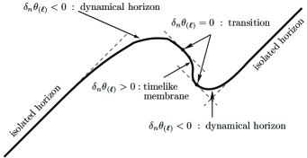
While dynamical horizons cannot violate the trapped surface extremality condition, they can transform into a new type of structure that does not contain trapped surfaces inside. In Booth et al. (2006), it is demonstrated that marginally trapped tubes (foliated three-surfaces which satisfy and ) in Tolman-Bondi spacetimes may transform from being spacelike (and so dynamical horizons with ) to timelike (with ). The change in behaviour occurs when the dust density becomes greater than where is the area of the horizon cross-sections. Intuitively one can think of this as occurring when the matter density becomes high enough to form a new horizon outside the old and then the timelike section of the horizon is characteristic of a horizon “jump”. Such a behaviour is shown in Fig. 2 (which is adapted from Booth et al. (2006)).
Similarly, Schnetter, Krishnan, and Florian Schnetter et al. (2006) have studied various numerical simulations including the collision of spinning black holes. They find that before the holes collide, an outer spacelike horizon forms. At the same time, an inner horizon forms which is part spacelike, part timelike. Although they were unable to follow the evolution far enough, they conjecture that the horizons will form a continuous three-surface, only some fraction of which is spacelike. The results presented here suggest a criterion for determining when these jumps are about to occur — the transition between the spacelike and timelike sections of the horizon will occur as . Note however that in general this transition may be complicated and include horizon cross-sections whose evolution may be spacelike in some areas and null or timelike in others. For a detailed understanding of the transition one would need to track and/or the signature of the evolution vector point-by-point. However while the evolution is still purely spacelike, should provide a good estimate of the proximity to extremality.
With a view towards tracking either or in a simulation, let us reformulate the expressions above in terms of spacelike/timelike unit normals. First, in terms of the unit tangent () and normal () vectors to the horizon, the angular momentum one-form and stress-energy component can be rewritten as
| (50) |
for the preferred scaling (44) where is the extrinsic curvature of the horizon relative to .
Alternatively we can consider an apparent horizon, with unit normal , in a three-slice , with unit timelike normal . The horizon evolution vector field can be expressed as
| (51) |
where is the lapse and is the the velocity of the horizon relative to the foliation. Then, following Booth (2007), we can write
| (52) |
where and so . We obtain a similar expression for the extremality parameter as:
See Ref. Booth (2007) for further details of these calculations.
Thus, thanks to the preferred scaling of the null normals we have an unambiguous definition of on each slice of any dynamical horizon. Things are, however, slightly more complicated in more general situations. First, keep in mind that the scalings (44) are defined by the timelike normal to and the spacelike normal to in . Thus one cannot use this form of the definition if becomes null (either as an isolated horizon or while transitioning to become a timelike membrane). In such cases one must return to the original definition Eq. (21).
There is also a second situation where it is not feasible to use Eq. (IV) to calculate . An apparent horizon in a set of initial data can evolve into many different dynamical horizons depending on how the data itself is evolved – that is apparent horizons are foliation dependent. From the point of view of Eq. (IV) the various potential horizons will generate different scalings of the null normals to and so different values of . This ambiguity can be more easily understood by switching back to the original definition of the extremality parameter given in Eq. (21). Then, if and the ambiguity in under rescalings of the null vectors is given by
| (54) |
while
| (55) |
That said, it should be kept in mind that by the trapped surface classification presented in Section III.3, is defined as sub-extremal, extremal, or super-extremal based on possible rather than any particular scalings of the null vectors. Though may vary for various choices of scalings, the ultimate classification of is invariant. For dynamical horizons a suitable scaling is defined by the normals to , but if one only has a single surface, then one must go back to an analysis of the elliptic operator defined by Eq. (55).
Interestingly, in the context of trapping horizons, Hayward Hayward (1994) has introduced an alternative expression for surface gravity which is proportional to . Such a definition explicitly ties together the non-vanishing of surface gravity with the existence of trapped surfaces inside the horizon, i.e. the second and third characterizations of extremality necessarily coincide. Furthermore, making use of Eq. (III.2) he has obtained a zeroth law for trapping horizons which has many similarities with the extremality condition introduced in this paper.
V Summary
In this paper, we have considered three characterizations of extremality. The first is the standard Kerr bound on angular momentum relative to mass. We have argued that in general it is not well-posed due to the difficulties in defining mass and angular momentum in general relativity. Even when the Kerr bound is reformulated in terms of horizon area and angular momentum, it can only be meaningfully evaluated on axi-symmetric horizons. Furthermore, while we have not provided an explicit violation of this bound in asymptotically flat spacetimes, we have argued that it is likely that it can be violated. In particular Kerr-AdS solutions can violate the bound by an arbitrary amount. These results do not violate the recent theorems of Dain which only apply to asymptotically flat vacuum spacetimes.
A more satisfactory characterization of extremality for isolated horizons arises from the surface gravity. For isolated horizons, a sub-extremal horizon will have positive surface gravity, while the surface gravity for an extremal horizon vanishes. Furthermore, non-negativity of surface gravity leads to a bound on the integrated square of the angular momentum density and the matter stress-energy at the horizon.
Alternatively, we can characterize non-extremality as the requirement that there should be fully trapped surfaces just inside a black hole horizon. This notion is then applicable to both isolated and dynamical horizons. In addition, this condition again leads to a bound on the integrated square of the angular momentum density and the matter stress-energy at the horizon. The surface gravity and trapped surface characterizations of extremality for isolated horizons are very closely related, and indeed in axi-symmetry are entirely equivalent.
The local extremality condition is also sufficient to place a restriction on the maximum allowed angular momentum relative to the intrinsic geometry of the horizon. For horizons whose cross-sections can be embedded in Euclidean this is sufficient to imply the standard Kerr bound , however for more exotic intrinsic geometries we can only show that for some constant which may be made arbitrarily large in, for example, Kerr-AdS.
Thus, the notion of extremality extends beyond the Kerr solutions though in a non-trivial way. The spirit of the bounds remains. The angular momentum of the horizon is bounded relative to the intrinsic geometry of the horizon. In general, when no axis of rotation exists, it is the square of the angular momentum density which is bounded. Equivalently, one can think of this as a bound on the sum of the multipole moments of the angular momentum rather than the dipole itself. The extremality quantity, , which we have introduced should be calculable on apparent horizons occuring in numerical relativity simulations and would provide an interesting characterization of how close to extremality a black hole is immediately following a merger.
Acknowledgements
We would like to thank Peter Booth, Patrick Brady, Jolien Creighton, Herb Gaskill and Badri Krishnan for helpful discussions. Ivan Booth was supported by the Natural Sciences and Engineering Research Council of Canada. Stephen Fairhurst was supported by NSF grant PHY-0200852 and the Royal Society.
Appendix A Kerr anti-deSitter black holes
The Kerr-(anti)deSitter family of solutions are described by the metric:
| (56) | |||||
where
| (57) |
is the cosmological constant (and so is positive for deSitter and negative for anti-deSitter), is the mass parameter, and is the rotation parameter.
We are interested in the black hole sector of the solution space. The various horizons occur at the roots of . For , has four roots in the black hole sector. In increasing order they are a (negative) unphysical solution, inner black hole horizon, outer black hole horizon, and the cosmological horizon. For there are just two roots: the inner and outer black hole horizons. Our interest is in the outer black hole horizon which we label . The coordinate representation (56) of the metric diverges at but for our purposes we can work around this by considering appropriate limiting cases which are well-defined. Then, one can show (see for example Dehghani and Mann (2001)) that the areal radius and angular momentum of the horizon are, respectively,
| (58) |
Here, for definiteness, we focus on the extremal horizons of this family where the inner and outer horizons coincide and so has a degenerate root (the second and third roots are degenerate for ). Such cases are most easily identified by examining where the discriminant of vanishes (the expression is a quintic in and quartic in but may be dealt with easily enough with the help of a computer algebra system).
For a given value of the mass , there is a finite range of for which extremal solutions exist. The lower bound is where (this is a lower bound as for the signature of the the coordinate changes and becomes timelike close to and ). The maximum value occurs when the inner and outer black hole horizons and the cosmological horizon all coincide in a triply degenerate root.
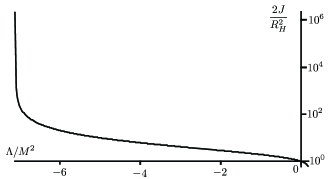
Given the range of values of which permit an extremal horizon, we can plot and see whether the extremality bound (19) is violated. This is shown in Fig. 3 and it is clear that the bound is violated for all extremal Kerr-AdS solutions. To understand this in light of the discussion in Section III.4, first note that in the presence of a cosmological constant Eq. (21) becomes:
| (59) |
Thus for , the contribution from the cosmologicl constant is positive and so we still have . In this case however becomes arbitrarily large as we approach . Specifically, the induced metric on a cross-section of the horizon is
| (60) |
Then the circumferential radius is
| (61) |
and
| (62) |
It is easy to see that this quantity diverges as .
For simplicity we only considered extremal horizons here, but it is clear (by continuity) that these violations of the bound will also extend into parts of the non-extremal sector.
Finally, it is perhaps interesting to note that on inserting a into Eq. (59), we see that the upper bound on the integral of increases with increasing . However, at least for Kerr-dS this does not provide enough freedom to violate as there is a concomitant tightening of .
Appendix B Surface of maximum
Let be the set of continuous functions that satisfy
-
i)
-
ii)
,
-
iii)
and and
-
iv)
for some .
Thinking back to the two-surfaces defined by these , the first condition guarantees a non-negative “radius”, the second and third require that the surfaces close exactly at and , and the fourth is the assumed bound on the maximum rate of change of the radius relative to the arclength.
Further define
Then in this appendix we show that of all , the triangular function
| (65) |
shown in Fig. 4 maximizes .
This is slightly more complicated than a basic variational problem. As noted in the text, if one generalizes to the set of all non-negative functions then is unbounded. Thus, our goal is to show that is globally maximized over by the “boundary” curve .
To prove this we first show that gives a local maximum. To this end, we calculate the first variation of in as
| (66) |
where all integrals are from to . For variations around this becomes
| (67) |
Now by the restriction on the maximum slope, all allowed and further is non-increasing from to . Thus taking (the zero of ) as a dividing point , we have for and for . Similar results apply for which is also non-increasing on this interval. Then, keeping in mind that must be zero at least somewhere we find . That is, all allowed variations decrease the value of and so provides at least a local maximum for our problem.
We complete the proof by showing for any other we can find a -increasing variation . It will be sufficient to restrict our attention to the subset of variations for which . For such variations (66) simplifies and we find
| (68) |
Intuitively these inequalities can be satisfied by constructing variations which increase where it is larger and balancing this off by decreasing it where it is smaller.
First consider the case where there is an interval over which is monotonically increasing but and construct a variation
| (72) |
where is arbitrarily small; in particular it is sufficiently small to ensure that and . By the monotonicity for and for , so by (68) it is straightforward to see that . Thus any that contains an increasing region over which , cannot maximize . A nearly identical argument shows that an with a decreasing region over which cannot provide a maximum.
In fact the same variation (72) can also be used to eliminate all which contain a constant section over which . In that case vanishes but a straightforward calculation of the second variation shows that this is because such a is a local minimum with respect to these variations.
Thus a which maximizes must have slope everywhere – that is either or a (possibly broken) “saw-toothed” curve such as that shown in Fig. 4.
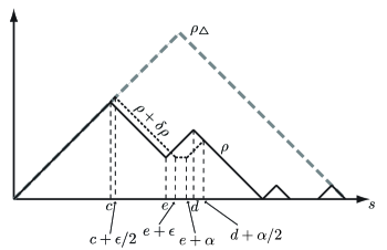
There are several special cases to consider here but while details differ, the basic variation is the same: we increase a higher peak while decreasing a lower one and so increase . In the interests of saving space we consider only the case of two immediately adjoining peaks as shown in the figure.
Then, with the higher peak at , lower at and the valley in between at we consider variations of the following type:
| (79) |
is the usual small parameter and is chosen so that . To first order (which is all that is needed for a variational calculation) it is
| (80) |
Then a direct calculation with (68) shows that if the first peak is higher than the second, . If they are equal then but going to the second order variation, it can be seen that this is because it is a local minimum under such variations. Similarly ponderous calculations can be performed to show that no other “saw-toothed” is a maximum.
Thus in summary we have shown that is a local maximum for curves in while there exist variations of all other curves that increase . Thus, is the global maximum as claimed.
References
- Dain (2006a) S. Dain (2006a), eprint gr-qc/0606105.
- Dain (2006b) S. Dain, Phys. Rev. Lett. 96, 101101 (2006b), eprint gr-qc/0511101.
- Dain (2006c) S. Dain, Class. Quant. Grav. 23, 6845 (2006c), eprint gr-qc/0511087.
- Ansorg and Petroff (2005) M. Ansorg and D. Petroff, Phys. Rev. D72, 024019 (2005), eprint gr-qc/0505060.
- Ansorg and Petroff (2006) M. Ansorg and D. Petroff, Class. Quant. Grav. 23, L81 (2006), eprint gr-qc/0607091.
- Petroff and Ansorg (2005) D. Petroff and M. Ansorg (2005), eprint gr-qc/0511102.
- Szabados (2004) L. B. Szabados, Living Rev. Rel. 7, 4 (2004).
- Hayward (1994) S. A. Hayward, Phys. Rev. D49, 6467 (1994).
- Hayward (2004a) S. A. Hayward, Phys. Rev. D70, 104027 (2004a), eprint gr-qc/0408008.
- Hayward (2006a) S. A. Hayward (2006a), eprint gr-qc/0607081.
- Hayward (2004b) S. A. Hayward, Phys. Rev. Lett. 93, 251101 (2004b), eprint gr-qc/0404077.
- Ashtekar et al. (1999) A. Ashtekar, C. Beetle, and S. Fairhurst, Class. Quant. Grav. 16, L1 (1999), eprint gr-qc/9812065.
- Ashtekar et al. (2000a) A. Ashtekar, C. Beetle, and S. Fairhurst, Class. Quant. Grav. 17, 253 (2000a), eprint gr-qc/9907068.
- Ashtekar et al. (2000b) A. Ashtekar, S. Fairhurst, and B. Krishnan, Phys. Rev. D62, 104025 (2000b), eprint gr-qc/0005083.
- Ashtekar et al. (2000c) A. Ashtekar et al., Phys. Rev. Lett. 85, 3564 (2000c), eprint gr-qc/0006006.
- Ashtekar et al. (2001) A. Ashtekar, C. Beetle, and J. Lewandowski, Phys. Rev. D64, 044016 (2001), eprint gr-qc/0103026.
- Ashtekar and Krishnan (2002) A. Ashtekar and B. Krishnan, Phys. Rev. Lett. 89, 261101 (2002), eprint gr-qc/0207080.
- Ashtekar and Krishnan (2003) A. Ashtekar and B. Krishnan, Phys. Rev. D68, 104030 (2003), eprint gr-qc/0308033.
- Booth and Fairhurst (2004) I. Booth and S. Fairhurst, Phys. Rev. Lett. 92, 011102 (2004), eprint gr-qc/0307087.
- Kavanagh and Booth (2006) W. Kavanagh and I. Booth, Phys. Rev. D74, 044027 (2006), eprint gr-qc/0603074.
- Booth and Fairhurst (2007) I. Booth and S. Fairhurst, Phys. Rev. D75, 084019 (2007), eprint gr-qc/0610032.
- Ashtekar and Galloway (2005) A. Ashtekar and G. J. Galloway, Adv. Theor. Math. Phys. 9, 1 (2005), eprint gr-qc/0503109.
- Lewandowski and Pawlowski (2003) J. Lewandowski and T. Pawlowski, Class. Quant. Grav. 20, 587 (2003), eprint gr-qc/0208032.
- Penrose (1965) R. Penrose, Phys. Rev. Lett. 14, 57 (1965).
- Israel (1986) W. Israel, Phys. Rev. Lett. 57, 397 (1986).
- Ashtekar et al. (2002) A. Ashtekar, C. Beetle, and J. Lewandowski, Class. Quant. Grav. 19, 1195 (2002), eprint gr-qc/0111067.
- Booth and Fairhurst (2005) I. Booth and S. Fairhurst, Class. Quant. Grav. 22, 4515 (2005), eprint gr-qc/0505049.
- Brown and York (1993) J. D. Brown and J. York, James W., Phys. Rev. D47, 1407 (1993).
- Dreyer et al. (2003) O. Dreyer, B. Krishnan, D. Shoemaker, and E. Schnetter, Phys. Rev. D67, 024018 (2003), eprint gr-qc/0206008.
- Schnetter et al. (2006) E. Schnetter, B. Krishnan, and F. Beyer, Phys. Rev. D74, 024028 (2006), eprint gr-qc/0604015.
- Hayward (2006b) S. A. Hayward, Phys. Rev. D74, 104013 (2006b), eprint gr-qc/0609008.
- Cook and Whiting (2007) G. B. Cook and B. F. Whiting (2007), eprint arXiv:0706.0199 [gr-qc].
- Korzynski (2007) M. Korzynski (2007), eprint arXiv:0707.2824 [gr-qc].
- Christodoulou (1970) D. Christodoulou, Phys. Rev. Lett. 25, 1596 (1970).
- Myers and Perry (1986) R. C. Myers and M. J. Perry, Ann. Phys. 172, 304 (1986).
- Emparan and Myers (2003) R. Emparan and R. C. Myers, JHEP 09, 025 (2003), eprint hep-th/0308056.
- Ansorg and Pfister (2007) M. Ansorg and H. Pfister (2007), eprint arXiv:0708.4196 [gr-qc].
- Pawlowski et al. (2004) T. Pawlowski, J. Lewandowski, and J. Jezierski, Class. Quant. Grav. 21, 1237 (2004), eprint gr-qc/0306107.
- Fairhurst and Krishnan (2001) S. Fairhurst and B. Krishnan, Int. J. Mod. Phys. D10, 691 (2001), eprint gr-qc/0010088.
- Ashtekar et al. (2004) A. Ashtekar, J. Engle, T. Pawlowski, and C. Van Den Broeck, Class. Quant. Grav. 21, 2549 (2004), eprint gr-qc/0401114.
- Newman (1987) R. P. A. C. Newman, Classical and Quantum Gravity 4, 277 (1987).
- Gourgoulhon (2005) E. Gourgoulhon, Phys. Rev. D72, 104007 (2005), eprint gr-qc/0508003.
- Gourgoulhon and Jaramillo (2006) E. Gourgoulhon and J. L. Jaramillo, Phys. Rev. D74, 087502 (2006), eprint gr-qc/0607050.
- Korzynski (2006) M. Korzynski, Phys. Rev. D74, 104029 (2006), eprint gr-qc/0605019.
- Eardley (1998) D. M. Eardley, Phys. Rev. D57, 2299 (1998), eprint gr-qc/9703027.
- Senovilla (2003) J. M. M. Senovilla, JHEP 11, 046 (2003), eprint hep-th/0311172.
- Booth et al. (2006) I. Booth, L. Brits, J. A. Gonzalez, and C. Van Den Broeck, Class. Quant. Grav. 23, 413 (2006), eprint gr-qc/0506119.
- Booth (2007) I. Booth (2007), eprint arXiv:0709.0934 [gr-qc].
- Dehghani and Mann (2001) M. H. Dehghani and R. B. Mann, Phys. Rev. D64, 044003 (2001), eprint hep-th/0102001.