Ordering from frustration in a strongly correlated one-dimensional system

Abstract

We study a one-dimensional extended Hubbard model with longer-range Coulomb interactions at quarter-filling in the strong coupling limit. We find two different charge-ordered (CO) ground states as the strength of the longer range interactions is varied. At lower energies, these CO states drive two different spin-ordered ground states. A variety of response functions computed here bear a remarkable resemblance to recent experimental observations for organic TMTSF systems, and so we propose that these systems are proximate to a QCP associated with $T=0$ charge order. For a ladder system relevant to $Sr_{14}Cu_{24}O_{41}$, we find in-chain CO, rung-dimer, and orbital antiferromagnetic ordered phases with varying interchain couplings and superconductivity with hole-doping. RPA studies of many chains (ladders) coupled reveal a phase diagram with the ordered phase extended to finite temperatures and a phase boundary ending at a quantum critical point (QCP). Critical quantum fluctuations at the QCP are found to enhance the transverse dispersion, leading to a dimensional crossover and a $T=0$ decofinement transition.

1 Introduction

Electron crystallization, or the charge ordering of electrons due to interactions, is an issue of enduring interest in condensed matter physics  mott ; imada . A host of excellent studies clearly show the relevance of charge ordering (CO) in diverse systems like organics org , transition metal oxides imada ; salamon , and coupled chain-ladder systems mccaron . Generically, CO seems to compete with superconductivity org ; mccaron , or with metallicity imada ; salamon . Hence, in addition to its intrinsic academic interest, the study of the conditions favoring CO, along with its competition with metallic (magnetic) and/or superconducting states constitutes a problem of wide-ranging interest for a host of real systems.

The simplest case of a CO state is the one where band fermions hop on a lattice with a staggered (static) crystal potential ashcroft . In this case, the CO gap is just the band-insulating gap. Needless to say, this picture is too simple; it does not contain the ingredients necessary to study the coupled charge/spin aspects of the systems mentioned above: these point to the basic importance of the Hubbard $U$ in practice. In contrast to the band-CO case, one expects the correlation driven CO state to have drastic consequences for the magnetic order emerging at lower energy scales imada ; org ; salamon ; mccaron , as well as for the competition between charge and spin orders manifested as one between Mott insulating (magnetic) and metallic (superconducting) states.

The availability of several powerful analytical as well as numerical methods in one dimension facilitates the detailed study of the effects of strong correlations in such systems. The study of the Hubbard model in one dimension, with and without extended Coulomb interactions, has a long history giamarchi ; capponi . With the focus mostly on the case of $1/2$-filling tsuchiizu , systems away from $1/2$-filling have not received sufficient attention. Furthermore, studies at different fillings have typically concentrated on the weak coupling limit yoshioka ; tsuorig ; yoshi1 , while real systems of interest imada ; org ; salamon ; mccaron are generically in the strong coupling limit of appropriate Hubbard-type models. Additionally, one dimensional correlated models with couplings to the lattice have also been studied riera ; kuwabara ; yoshi2 , revealing phase diagrams with various different kinds of charge orders (CO) and spin orders (SO).

The issue of whether various types of CO can, at fillings away from $1/2$, be driven purely by longer range Coulomb interactions remains, however, largely unadressed. The importance of extended Coulomb interactions was appreciated in an early work by Hubbard hubbard . Here, it was shown that the next nearest neighbor Coulomb (nnn) interaction can be as large as 40 percent of the nearest neighbor (nn) interaction, with the intra-atomic Hubbard $U$ being the largest, and the one-particle hopping between neighbors the smallest energy scales in an effective one-band extended Hubbard model. In practice, coupling to high-energy Einstein (optical) phonons has the result of reducing the nn coupling kuwabara ; in a model with Coulomb interactions extended to next nearest neighbours, this gives rise to the possibility of tuning the ratio of nnn to nn interactions through $1/2$, a point at which interesting additional physics is expected. Thus, the search for competing charge ordered states driven purely by long-range electronic interactions, and the co-existence of charge and spin order, in a one dimensional $1/4$-filled electronic model are among the primary goals of the present work. Further, by working with a model in which the Coulomb correlations are much larger than the single particle hopping strength, we are able to obtain analytic results in a regime where little progress has been made. From our earlier discussion, our results are also clearly relevant to several material systems.

In the following section, we begin by presenting a derivation of a 1D transverse field Ising model (TFIM) effective pseudospin Hamiltonian in the extreme strong-coupling limit for the charge degrees of freedom of the $1/4$-filled 1D spinful electron Hubbard model with extended correlations. We then discuss the consequences various features of the phase diagram of the (exactly solvable) TFIM effective model have for the charge and spin degrees of freedom of the original electronic model. Various thermodynamic quantities of the electronic model, e.g., the optical conductivity, the dielectric function and the electronic contribution to the Raman scattering, are computed from the effective pseudospin theory. We follow this, in section III, with an analysis of the effective theories obtained for the case of a 2-leg ladder of two coupled TFIM chains with the inter-chain couplings in the strong coupling limit, as well as for a ladder doped with holes. In section IV, we then analyse the case of many such TFIM (chain and 2-leg ladder) systems coupled to another by a random phase approximation (RPA) method giamarchi ; scalapino ; schulz ; carr . The goal is to conduct a systematic study of the physics of dimensional crossover and deconfinement in such anisotropic strongly coupled lower dimensional systems, when coupled to one another. In section V, we present a comparison of our findings with some recent numerical works. Finally, we conclude in section VI.

2 Single chain in strong-coupling regime

In this work, we study this issue within an extended quarter-filled Hubbard model on a linear chain, described by,

$$H_{\mathrm{eff}} = -t\sum_{i,\sigma}(C_{i\sigma}^{{\dagger}}C_{i+1,\sigma}+h.c)+(U-2zP)\sum_{i}n_{i\uparrow}n_{i\downarrow}$$ (1)

$$+V\sum_{i}n_{i}n_{i+1}+P\sum_{i}n_{i}n_{i+2}$$

The couplings $U$, $V$ and $P$ represent the on-site Hubbard, nn and nnn replusive interactions, $t$ represents the hopping strength and $z$ the coordination number for the lattice (which in the case of the linear chain is 2). This somewhat complicated looking microscopic model gives us the means to model extended Coulomb interactions in a $1/4$-filled system in the limit of strong coupling (as discussed below). Further, it is by now a well accepted paradigm that in theories of electrons in one-dimension interacting with one another through well-behaved (i.e., non-singular) potentials, the low-energy effective (fixed point) theory is one where the charge and spin degrees of freedom have separate dynamics  giamarchi . This is the concept of the Tomonaga-Luttinger liquid with spin-charge separation, and characterised by the spin fluctuations being those of an ideal $S=1/2$ XXX AF chain

$$H_{s}=J\sum_{j}{\bf S}_{j}.{\bf S}_{j+1},$$ (2)

while the charge fluctuations are described by the Hamiltonian

$$H_{\mathrm{c}} = -t\sum_{i}(c_{i}^{{\dagger}}c_{i+1}+h.c)+(V-J/4)\sum_{i}n_{i}n_{i+1}$$ (3)

$$+P\sum_{i}n_{i}n_{i+2}$$

that describes a model with frustrating interactions. The coupling $J$ is obtained from straightforward perturbation theory as $J\sim 4t^{2}/(U-V-4P)$. In 1D, the projected fermions are spinless fermions with a hard-core constraint.

2.1 Effective TFIM model

The model for spinless electrons given above has been considered as a model for studying the effects of frustration on charge ordering emery ; kats . For narrow-band systems, we consider the limit $t<<(V-J/4),P$. Before embarking on a detailed derivation of the effective Hamiltonian in this regime, we present a heuristic one emery . For this, we employ an extension of the trick used for the $1d$ next-nearest neighbor Ising chain: for $t=0$, we notice that with $(V-J/4)>2P$, the ground state is the usual CDW (Wigner) crystal (and doubly degenerate, (..101010…) and (…010101…), for $1/4$-filling). With $2P>(V-J/4)$, however, the dimerized state (Peierls) is the ground state. The ground state has a degeneracy of four, with one of the states written schematically as (11001100….) and the other three achieved by shifting the state by one lattice site. Taking the state shown and splitting this in a slightly different way, we have […(01)(10)(01)(10)…]. Associating a pseudospin $\tau=1/2$ operator, with $\tau^{z}=+1$ for (10) and -1 for (01), the state is antiferromagnetic and doubly degenerate in terms of the $\tau_{i}^{z}$. This state has a partner, obtained by shifting the state given above by 2 sites (or the pseudospin $\tau$ variables by one site). For small $t$, this is an attractive trick because (in spin language) the transverse term does flip the $\tau_{i}^{z}$, but cannot break a pair. This leads to the effective Hamiltonian emery ; kats ,

$$H_{\mathrm{eff}}=-\sum_{l}[2t\tau_{l}^{x}+(V-J/4-2P)\tau_{l}^{z}\tau_{l+1}^{z}]$$ (4)

Let us now see how this simple Hamiltonian is obtained as the effective Hamiltonian for our original theory for the charge degrees of freedom in the limit of the couplings $U>>V,P>>t$. We begin with the Hamiltonian for a spin chain system

$$H = -\sum_{n}[J_{x}(S_{n}^{x}S_{n+1}^{x}+S_{n}^{y}S_{n+1}^{y})+J_{1}S_{n}^{z}S_{n+1}^{z}$$ (5)

$$+J_{2}S_{n}^{z}S_{n+2}^{z}+hS_{n}^{z}]$$

where $S_{n}^{x}$, $S_{n}^{y}$ and $S_{n}^{z}$ and spin-1/2 operators. The couplings $J_{x}$, $J_{1},J_{2}>0$ are the nearest neighbour (nn) XY, the nearest neighbour Ising and the next nearest neighbour (nnn) Ising couplings respectively and $h$ is the external magnetic field. For $h=0$, this Hamiltonian can be derived from the on-site Hubbard interaction $U\rightarrow\infty$ strong-coupling limit of an extended Hubbard model at 1/4-filling and with nn ($J_{1}\equiv(V-J/4)$) and nnn ($J_{2}\equiv 2P$) density-density interaction couplings and the nn electron hopping ($J_{x}\equiv t$) via a Jordan-Wigner transformation (from a model of spinless-fermions to spins)

$$H=\sum_{n}[-\frac{J_{x}}{2}(c_{i}^{\dagger}c_{i+1}+h.c)+J_{1}n_{i}n_{i+1}+J_{2}n_{i}n_{i+2}]~{}.$$ (6)

We study the problem in the limit of strong-coupling where $J_{1},J_{2}>>J_{x}$ (but where $(J_{1}-2J_{2})\sim 2J_{x}$).

Let us begin by studying the case of $J_{x}=0$ emery (we will be studying eq.(5) for the case of $h=0$ in all that follows). It is easy to see that for the case of $J_{1}>2J_{2}$, the ground state of the system is given by a Neel-ordered antiferromagnetic (AF) state with two degenerate ground-states given by

$$|AFGS1\rangle = |\ldots+-+-+-+-\ldots\rangle$$

$$|AFGS2\rangle = |\ldots-+-+-+-+\ldots\rangle$$ (7)

where we signify $S_{n}^{z}=1/2,-1/2$ by $+$ and $-$ respectively and we have explicitly shown the spin configuration in the site nos. $-3\leq n\leq 4$ in the ground states. In the original electronic Hamiltonian eq.(6), this AF order corresponds to a Wigner charge-ordering (CO) in the ground-state. Similarly, for the case of $J_{1}<2J_{2}$, the ground state of the system is given by a dimer-ordered $(2,2)$ state emery with four degenerate ground-states given by

$$|22GS1\rangle = |\ldots-++--++-\ldots\rangle$$

$$|22GS2\rangle = |\ldots--++--++\ldots\rangle$$

$$|22GS3\rangle = |\ldots+--++--+\ldots\rangle$$

$$|22GS4\rangle = |\ldots++--++--\ldots\rangle$$

where we signify $S_{n}^{z}=1/2,-1/2$ by $+$ and $-$ respectively and we have explicitly shown the spin configuration in the site nos. $-2\leq n\leq 5$ in the ground states. In the original electronic Hamiltonian eq.(6), this $(2,2)$ order corresponds to a Peierls CO in the ground-state. Further, as the Hamiltonian eq.(5) with $J_{x}=0=h$ is the one-dimensional axial next nearest neighbour Ising (ANNNI) model, we know that the “frustration” point at $J_{1}=2J_{2}$ peschel is gapless, highly degenerate and has a ground state entropy per site of $\ln(1+\sqrt{5})/2\simeq 0.4812$ while the ordered ground states on either side of the frustration point have zero ground state entropy liebmann .

We now work out the effect of the XY terms in the Hamiltonian (5) on these ground states. Let us start with noting the effect of a XY term on a single nn spin-pair on the 4 degenerate $(2,2)$ ground-states; for purposes of brevity, we will denote the entire $J_{x}(S_{n}^{x}S_{n+1}^{x}+S{n}^{y}S_{n+1}^{y})$ term simply as $J_{x}^{n,n+1}$. Thus,

$$J_{x}^{0,1}|22GS1\rangle = J_{x}^{0,1}|\ldots+-\ldots\rangle=\frac{J_{x}}{2}|\ldots-+\ldots\rangle$$

$$J_{x}^{0,1}|22GS2\rangle = J_{x}^{0,1}|\ldots++\ldots\rangle=0$$

$$J_{x}^{0,1}|22GS3\rangle = J_{x}^{0,1}|\ldots-+\ldots\rangle=\frac{J_{x}}{2}|\ldots+-\ldots\rangle$$

$$J_{x}^{0,1}|22GS1\rangle = J_{x}^{0,1}|\ldots--\ldots\rangle=0$$

$$J_{x}^{-1,0}|22GS1\rangle = J_{x}^{-1,0}|\ldots++\ldots\rangle=0$$

$$J_{x}^{-1,0}|22GS2\rangle = J_{x}^{-1,0}|\ldots-+\ldots\rangle=\frac{J_{x}}{2}|\ldots+-\ldots\rangle$$

$$J_{x}^{-1,0}|22GS3\rangle = J_{x}^{-1,0}|\ldots--\ldots\rangle=0$$

$$J_{x}^{-1,0}|22GS4\rangle = J_{x}^{-1,0}|\ldots+-\ldots\rangle=\frac{J_{x}}{2}|\ldots-+\ldots\rangle~{}.$$ (9)

In a similar manner, we study the action of the operator $J_{x}^{n,n+1}$ on the two degenerate ground states of the AF ordered configuration as

$$J_{x}^{0,1}|AFGS1\rangle = J_{x}^{0,1}|\ldots+-\ldots\rangle=\frac{J_{x}}{2}|\ldots-+\ldots\rangle$$

$$J_{x}^{0,1}|AFGS2\rangle = J_{x}^{0,1}|\ldots-+\ldots\rangle=\frac{J_{x}}{2}|\ldots+-\ldots\rangle$$

$$J_{x}^{-1,0}|AFGS1\rangle = J_{x}^{-1,0}|\ldots-+\ldots\rangle=\frac{J_{x}}{2}|\ldots+-\ldots\rangle$$

$$J_{x}^{-1,0}|AFGS2\rangle = J_{x}^{-1,0}|\ldots+-\ldots\rangle=\frac{J_{x}}{2}|\ldots-+\ldots\rangle~{}.$$ (10)

Defining bond-pseudospins $\tau_{i}^{z}=(S_{i}^{z}-S_{i-1}^{z})/2$, $\tau_{i}^{+}=S_{i}^{+}S_{i-1}^{-}$ and $\tau_{i}^{-}=S_{i}^{-}S_{i-1}^{+}$ (which can be rewritten in terms of fermionic operators in the original electronic Hamiltonian eq.(6) as $\tau_{i}^{z}=(n_{i}-n_{i-1})/2$, $\tau_{i}^{+}=c_{i}^{\dagger}c_{i-1}$ and $\tau_{i}^{-}=c_{i}c_{i-1}^{\dagger}$ respectively), we can write the four degenerate ground states of the $(2,2)$ ordered configuration in terms of these bond pseudospins as

$$|22GS1\rangle = |\ldots~{}0~{}-~{}0~{}+~{}0\ldots\rangle$$

$$|22GS2\rangle = |\ldots\hskip 2.84544pt+~{}0~{}-~{}0~{}+\ldots\rangle$$

$$|22GS3\rangle = |\ldots~{}0~{}+~{}0~{}-~{}0\ldots\rangle$$

$$|22GS4\rangle = |\ldots\hskip 2.84544pt-~{}0~{}+~{}0~{}-\ldots\rangle~{},$$ (11)

where we have denoted $\tau_{n}^{z}=1/2$ as $+$ and $\tau_{n}^{z}=-1/2$ as $-$ and have explicitly shown the pseudospin configurations on the bond nos. $0\leq n\leq 4$. We can clearly see from eq.(11) that these four ground-states break up into two pairs of doubly degenerate (AF) orderings of the pseudospins defined on the odd bonds ($|22GS1\rangle$ and $|22GS3\rangle$) on the even bonds ($|22GS2\rangle$ and $|22GS4\rangle$) respectively. It is also simple to see from eq.(9) that the action of the operator $J_{x}^{n-1,n}$ (for the nearest neighbour pair of sites given by $(n-1,n)$) on these four ground states is to flip a pseudospin defined on the bond $n$ (lying in between the pair of sites $(n-1,n)$) or to have no effect at all.

We can now similarly see that the two-degenerate ground states of the AF ordered configuration can be written in terms of the bond-pseudospins defined above as

$$|AFGS1\rangle = |\ldots+-+-+\ldots\rangle$$

$$|AFGS2\rangle = |\ldots-+-+-\ldots\rangle$$ (12)

where we have explicitly shown the pseudospin configurations on the bond nos. $0\leq n\leq 4$. From eq.(12), we see that the two degenerate ground-states have antiferromagnetic ordering of pseudospins on nn bonds; this can equally well be understood in terms of the ferromagnetic ordering of pseudospins on the odd bonds and on the even bonds separately. Further, from eq.(10), we can see that the action of the operator $J_{x}^{n-1,n}$ (for the nearest neighbour pair of sites given by $(n-1,n)$) on these two ground states is again to flip a pseudospin defined on the odd (even) bond $n$ (lying in between the pair of sites $(n-1,n)$) against a background of ferromagnetically ordered configuration of pseudospins defined on the odd (even) bonds.

Thus, we can model these pseudospin ordered ground states (11),(12) as well as all possible pseudospin-flip excitations above them (as given by action of operators of the type $J_{x}^{n-1,n}$ (9),(10)) with the effective Hamiltonian

$$H = -\sum_{n\in odd}[2J_{x}\tau_{n}^{x}+(J_{1}-2J_{2})\tau_{n}^{z}\tau_{n+2}^{z}]$$ (13)

$$-\sum_{n\in even}[2J_{x}\tau_{n}^{x}+(J_{1}-2J_{2})\tau_{n}^{z}\tau_{n+2}^{z}]$$

$$= -\sum_{n}[2J_{x}\tau_{n}^{x}+(J_{1}-2J_{2})\tau_{n}^{z}\tau_{n+2}^{z}]~{},$$

where $n$ is the bond index.

This is just the Ising model in a transverse field, which is exactly solvable lieb ; niemeijer and has been studied extensively in 1D  sachdev ; chakrabarti . If $(V-J/4-2P)>0$, the ground state is ferromagnetically ordered in $\tau^{z}$, i.e, it corresponds to a Wigner CDW. For $(V-J/4-2P)<0$, the Peierls dimer order results in the ground state. At $(V-J/4-2P)<2t$, the quantum disordered phase has short-ranged pseudospin correlations, and is a charge “valence-bond” liquid. The quantum critical point at $(V-J/4-2P)=2t$ separating these phases is a deconfined phase with gapless pseudospin ($\tau$) excitations, and power-law fall-off in the pseudospin-pseudospin correlation functions. Correspondingly, the density-density correlation function has a power-law singular behavior at low energy, with an exponent $\alpha=1/4$ characteristic of the $2D$ Ising model at criticality. The gap in the pseudospin spectrum on either side of the critical point is given by $\Delta_{\tau}=2|V-J/4-2P-2t|$. Further, the quantum-critical behaviour extends to temperatures as high as $T\sim\Delta_{\tau}/2$  kopp and undergoes finite-temperature crossovers to the two gapped phases at $T\sim|\Delta_{\tau}|$. For $P=0$, the metallic phase for $V-J/4\leq 2t$ is a Luttinger liquid, and in this limit, the low-energy physics is qualitatively similar to that of the usual $t-J$ model. The “Mott” insulating state for $V-J/4>2t$ has Wigner CO in the ground state, and the M-I transition is of the Kosterlitz-Thouless type tsvelik .

\psfrag{1}[bl][bl][4][0]{$T$}\psfrag{2}[bl][bl][4]{$g$}\psfrag{3}[bl][bl][3.5][0]{$g=0$}\psfrag{4}[bl][bl][3.5][0]{Low $T$ gapped}\psfrag{5}[bl][bl][3.5][0]{CO state}\psfrag{6}[bl][bl][3.5][0]{with LRO}\psfrag{7}[bl][bl][4][0]{Quantum}\psfrag{8}[bl][bl][4][0]{Critical}\psfrag{9}[bl][bl][3.5][0]{Low $T$ gapped}\psfrag{10}[bl][bl][3.5][0]{short ranged}\psfrag{11}[bl][bl][3.5][0]{charge VB liquid}\includegraphics{tfimphasediag.eps}

Figure 1: A schematic phase diagram of the temperature $T$ vs. coupling $g=|(V-J/4-2P-2t)/(V-J/4-2P)|=\Delta_{\tau}/(V-J/4-2P)$ of the effective 1D Transverse Field Ising Model theory for the charge sector of our original electronic model. The black circle with $g=0$ represents the $T=0$ quantum critical point (QCP) separating an phase with true LRO given by Wigner CDW or Peierls dimer order (depending on whether $V-J/4>2P$ or $V-J/4<2P$ respectively, thick dark line) and a quantum disordered phase corresponding to a charge valence bond (VB) liquid. The finite-$T$ physics of the quantum critical region lying just above the QCP is discussed in subsection IIB. The dashed regions represent finite-$T$ crossovers to low-$T$ gapped charge ordered and charge VB liquid phases with no long-range order (LRO).

The full Hamiltonian in our case for the strong-coupling limit is now given by

$$H_{\mathrm{eff}}=-\sum_{l}[2t\tau_{l}^{x}+(V-J/4-2P)\tau_{l}^{z}\tau_{l+1}^{z}]+J\sum_{l}{\bf S_{l}}.{\bf S_{l+1}}$$ (14)

To study the magnetic phases, we adapt the Ogata-Shiba ogata technique for our case. This is possible if $J(\sim t^{2}/(U-V-4P))<<t,V$, in which case, the pseudospin part is first solved exactly (this is possible because of the known exact solution of the 1D transverse field Ising model), and the exchange part is then treated as a perturbation. Writing the total wavefunction as a product of a spin and pseudospin wavefunction (where the spin wavefunction is defined, for a system of size $N$, in a Hilbert space of dimension $2^{N}$), i.e, $|\psi>=|\tau>\otimes|{S}>$, and following standard degenerate perturbation theory, the spin degeneracy is lifted by the correction (of order $1/N$):

$$<H_{\mathrm{eff}}>^{\prime}=-2t<\tau^{x}>+\sum_{l}\tilde{J}_{l,l+1}({\bf S_{l}}.{\bf S_{l+1}}-1/4)$$ (15)

where the average $<..>^{\prime}$ denotes that the average is taken over the exact ground state $|\tau>$ of the pseudospin part above, i.e. $<A>^{\prime}=<\tau|A|\tau>$ and $\tilde{J}_{l,l+1}=\frac{1}{N}(V-\frac{J}{4}-2P)<\tau_{l}^{z}\tau_{l+1}^{z}>$.

An interesting fact now emerges: Wigner CO (FM order of $\tau$) results in an HAFM $S=1/2$ spin model with the Hamiltonian $H_{\mathrm{s}}=\tilde{J}\sum_{i}{\bf S}_{i}.{\bf S}_{i+1}$. This gives rise to a gapless AF ground state for the spin degrees of freedom. The charge (holon) excitations have a gap $\Delta_{\tau}=2(V-J/4-2P-2t)$; this corresponds to a linear confining potential for holons. On the other hand, Peierls dimerization in the charge sector (AF Neel order of $\tau$) gives rise to dimerization in the spin sector, with the Hamiltonian $H_{\mathrm{s}}=\tilde{J}\sum_{i}[1+(-1)^{i}\delta]{\bf S}_{i}.{\bf S}_{i+1}$. The bare value of the dimerisation is given found from the perturbation theory as proportional to the Ising pseudospin (charge dimer) gap, i.e., $\delta\sim\Delta_{\tau}/\tilde{J}$. However, as we shall discuss now, a continuum field theoretic description of this Hamiltonian shows that the dimerisation parameter $\delta$ is renormalised by quantum fluctuations, and scales as $\delta\sim(\Delta_{\tau}/\tilde{J})^{2/3}$.

Translated into fermion variables, this yields a sine-Gordon problem with $\beta^{2}=2\pi$, and describes an instability to a singlet pinned ground state commensurate with the Peierls CO setting in at higher energies. The elementary excitations are solitons carrying $S^{z}=\pm 1$. Scaling theory predicts a dimer gap, $\Delta_{\tau}\simeq\delta^{2/3}\tilde{J}$. Exactly at $\beta^{2}=2\pi$, the SG model has just two $S^{z}=0$ breather excitations with opposite parity haldane , the lowest, even parity breather being degenerate with the $S^{z}=\pm 1$ soliton doublet, forming a $S=1$ triplet, while the second odd-parity breather is a singlet with a gap, $\sqrt{3}\Delta_{\tau}$. It is important to notice that both charge and spin order arise from long range Coulomb interactions, and do not involve an electron phonon coupling mechanism.

2.2 Consequences of CO on thermodynamic quantities in the quantum critical regime

Let us consider the implications of having the CO state in the high-$T$ regime, where one could imagine the system to be effectively one-dimensional. In particular, we want to look at the $\omega,T$ dependence of the various response functions at high-$T$. Using the exact solution of the pseudospin model in 1D, the high $T$ (in the “quantum critical” regime) behavior can be explicitly derived sachdev . In fact, near Ising criticality, the response function, $\chi(r)\simeq r^{-1/4}$ where $r=(x^{2}+\tau^{2})^{1/2}$ (with the velocity $v$ set to unity). This relation is still valid away from criticality in the “short range” region, $r<<\Delta_{\tau}$, where $\Delta_{\tau}=2|V-J/4-2P-2t|$ is the pseudospini gap (which corresponds, in our case, to the charge gap) of the 1D-TFIM. As we will see, in what follows, knowing the microscopic form of the Ising pseudospin gap $\Delta_{\tau}$ is enough information for us to be able to compute a host of thermodynamic response functions of the sytem and be able to relate them to the couplings in our original microscopic theory of interacting electrons in one dimension. Using this asymptotic form, we have

$$\chi_{\mathrm{crit}}(0,\omega)=-\frac{\sin(2\pi\Delta)}{(2\pi T)^{2-4\Delta}}B^{2}(\Delta-iS,1-2\Delta)$$ (16)

where $S=\frac{\omega}{4\pi T}$, and $\Delta=1/16$ is the conformal dimension. $B(x,y)$ is the beta function.

In the quantum critical region, an illuminating form is

$$\chi(k,\omega)=\frac{\chi(0,0)}{1-i\omega/\Gamma_{\mathrm{R}}+k^{2}\xi^{2}-(\omega/\omega_{1})^{2}}$$ (17)

where the quantities $\Gamma_{\mathrm{R}}=(2\tan(\pi/16)k_{\mathrm{B}}T/\hbar)e^{-\Delta_{\tau}/k_{\mathrm{B}}T}$, $\omega_{1}=0.795(k_{\mathrm{B}}T/\hbar)$ and $\xi=1.28(c\hbar/k_{\mathrm{B}}T)e^{\Delta_{\tau}/k_{\mathrm{B}}T}$, are determined solely by $T$ and the fundamental natural constants, as expected in the QC regime. We stress once again that here, $\Delta_{\tau}=2(V-J/4-2P-2t)$ is the energy gap to charge excitations in the Wigner/Peierls CO states (Ising pseudospin gap) described above. This represents the collective charge susceptibility, and the optical conductivity follows directly from $\sigma(\omega)=-i\omega\chi(0,\omega)$, giving,

$$\sigma(\omega)=\frac{\chi(0,0)}{\Gamma_{R}}\frac{\omega^{2}}{(1-\omega^{2}/\omega_{1}^{2})^{2}+(\omega/\Gamma_{\mathrm{R}})^{2}}$$ (18)

The frequency dependent dielectric function, $\epsilon(\omega)$, is obtained from $\epsilon(\omega)=1+(4\pi i\sigma(\omega)/\omega)$, and the electronic contribution to the Raman scattering is estimated therefrom to be given by $I_{\mathrm{R}}(\omega)=\mathrm{Im}(1/\epsilon(0,\omega))$, for light polarized along the chain axis. In terms of the charge susceptibility, this is simply,

$$I_{\mathrm{R}}(\omega)=\mathrm{Im}\frac{1}{\epsilon(\omega)}=\frac{\frac{4\pi\chi(0,0)}{\Gamma_{\mathrm{R}}}F(\omega,T)}{1+(\frac{4\pi\chi(0,0)}{\Gamma_{\mathrm{R}}})^{2}F^{2}(\omega,T)}$$ (19)

where $F(\omega,T)=\frac{\omega}{(1-\omega^{2}/\omega_{1}^{2})^{2}+(\omega/\Gamma_{\mathrm{R}})^{2}}$.

$\chi"(k,\omega)$ has its maximum value at $\omega_{m}=\omega_{1}-i(\omega_{1}^{2}/\Gamma_{\mathrm{R}})$, implying that the collective mode broadens and shifts to higher energy linearly in $T$ with increasing $T$ at high temperatures. Further, the $T$-dependent damping rate of the collective mode correlates well with the relaxational peak seen in transport, underlying their common origin. In fact, the $dc$ resistivity is linear in $T$ at high $T$, with “insulating” features showing up at lower $T$. In our picture, these are collective (longitudinal) bosonic charge-density modes in the high-$T$ quantum critical region above an incipient CO transition (expected to occur at low $T$). In fig.(1), we show the electronic Raman lineshape as a function of $\omega/T$. The sharp low energy peak corresponds to the collective charge density fluctuation mode of the CO ground state.

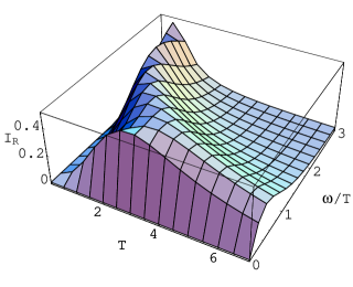
Figure 2: A three-dimensional plot of the Raman intensity $I_{R}$ versus a scaled energy $\omega/T$ and temperature $T$ for parameter values of the original model which constitute a gap $\Delta_{\tau}=0.05k_{\mathrm{B}}$.

The corresponding frequency-dependent dielectric constant also shows an explicit $\omega/T$ scaling in the QC regime, or generally, at high-$T$, it shows strong $T$-dependence. From fig.(2), we see that it becomes $\omega$-independent at high $T$, but appreciably increases as $T$ is lowered, with a maximum at $\omega\simeq T$.

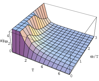
Figure 3: A three-dimensional plot of $\sigma(\omega)/\omega$ versus a scaled energy $\omega/T$ and temperature $T$ for $\Delta_{\tau}=0.05k_{\mathrm{B}}$. The limiting behaviors are: (1) $\sigma(\omega)\simeq\frac{\omega^{2}}{T^{11/4}}$ for high $T$, and $\sigma(\omega)\simeq\frac{1}{\omega^{3/4}}$ for low $T$. (2) $\epsilon^{\prime}(\omega,T)=1+\frac{const}{T^{7/4}}$ for high $T$, and $\epsilon^{\prime}(\omega,T)\simeq\frac{-1}{\omega^{7/4}}$ for low $T$.

The fact that organic charge transfer salts bra exhibit features very similar to those found above has interesting implications. In light of our results, these anomalous features can now be identified with proximity to an underlying quantum critical point associated with charge (Wigner/Peierls) ordering. We recall that very recent work mon ; bishop shows that the dimerized insulating state in TMTSF systems has charge order at low $T$. Interestingly, $\epsilon^{\prime}(0,\omega)$ indeed shows appreciable increase as $T$ is lowered, further supporting an interpretation based on proximity to an underlying CO ground state bra . Hence, we conclude that observation of these features in TMTSF systems constitutes strong evidence that this system is close to a putative QCP associated with charge order. Observation of dimerized/Neel ordered AFM states co-existing CO states at low $T$ are also naturally understood in light of the analysis above bishop .

3 Two-chain TFIM Ladder systems at strong inter-chain coupling

We now consider the strong coupling version of a coupled two-chain ladder system, with each chain being described by $H$ as in eq.(1). In the strong coupling limit, where each chain is described by a TFIM for charge degrees of freedom, the coupled chain model is constructed as follows. For $U\rightarrow\infty$, and $V,P>t$ (but $(V-J/4-2P)$ comparable to $t$), the charge degrees of freedom of the fermionic problem for each chain are described by an effective pseudospin model on n-n bonds, via the effective Hamiltonian,

$$H^{chain}=-\sum_{j}[2t\tau_{j}^{x}+(V-J/4-2P)~{}\tau_{j}^{z}\tau_{j+1}^{z}]$$ (20)

Rotating the pseudospin axis such that $\tau^{x}\rightarrow\tau^{z}$, $\tau^{z}\rightarrow-\tau^{x}$ and coupling two such chains via an interaction coupling $U_{\perp}$ and a two-electron interchain transfer $t_{\perp}$, we have the effective Hamiltonian for the charge sector of the two chain system as

$$H = -\sum_{j,a}[2t\tau_{j,a}^{z}+(V-J/4-2P)~{}\tau_{j,a}^{x}\tau_{j+1,a}^{x}]$$ (21)

$$-\sum_{j,a,b\neq a}[U_{\perp}\tau_{j,a}^{z}\tau_{j,b}^{z}+~{}t_{\perp}~{}(\tau_{j,a}^{x}\tau_{j,b}^{x}+\tau_{j,a}^{y}\tau_{j,b}^{y})]~{},$$

where $a,b=1,2$ is the chain index. Denote the in-chain pseudospin coupling as $J=(V-J/4-2P)$ and the inter-chain pseudospin coupling as $J_{\perp}=U_{\perp}$. Here, we study the strong coupling version of this problem in several limits by deriving the respective low-energy effective Hamiltonians (LEEH). The weak-coupling problem is studied elsewhere next .

3.1 The case of $|J_{\perp}|>>|J|,~{}t_{\perp}$

For the case of $|J_{\perp}|>>|J|,~{}t_{\perp}$ , the 2 chain system can be better thought of as strongly-coupled rungs which are weakly coupled to their neighboring rungs. Thus, we treat $J$ as a weak perturbation on the zeroth-order system of rungs defined by the large coupling $J_{\perp}$, giving $H_{eff}=H_{0}+H_{1}$ where

$$H_{0} = -h\sum_{j,a}\tau_{j,a}^{z}+J_{\perp}\sum_{j,a,b\neq a}\tau_{j,a}^{z}\tau_{j,b}^{z}$$

$$H_{1} = -J\sum_{j,a}\tau_{j,a}^{x}\tau_{j+1,a}^{x}-\frac{t_{\perp}}{2}\sum_{j,a,b\neq a}(\tau_{j,a}^{+}\tau_{j,b}^{-}+{\rm h.c})$$ (22)

where the effective magnetic field is given by $h=2t>0$.

3.1.1 LEEH for $J_{\perp}<0$

For $J_{\perp}<0$ and $h<<J_{\perp}$, we find that the triplet state $|+\rangle=\frac{1}{\sqrt{2}}(|\uparrow\downarrow\rangle+|\downarrow\uparrow\rangle)$ and the singlet state $|-\rangle=\frac{1}{\sqrt{2}}(|\uparrow\downarrow\rangle-|\downarrow\uparrow\rangle)$ are degenerate on any rung and are separated from all other states by a large gap of order $J_{\perp}$. Thus, these two states define the subspace which will determine the low-energy physics of the system. Identifying a pseudospin-1/2 operator $\xi_{j}$ with the low-energy subspace on each rung, we treat the Hamiltonian $H_{1}$ as a perturbation (to second order in $J/J_{\perp}$) to obtain the LEEH as

$$H = \sum_{j}[-\frac{J^{2}}{2J_{\perp}}(\frac{J_{\perp}^{2}-2h^{2}}{J_{\perp}^{2}-4h^{2}})\xi_{j}^{z}\xi_{j+1}^{z}-\frac{t_{\perp}}{2}\xi_{j}^{z}$$ (23)

$$-\frac{J^{2}}{2J_{\perp}}(\frac{h^{2}}{J_{\perp}^{2}-4h^{2}})(\xi_{j}^{+}\xi_{j+1}^{+}+{\rm h.c})-\frac{J^{2}}{8J_{\perp}}(\frac{J_{\perp}^{2}-2h^{2}}{J_{\perp}^{2}-4h^{2}})]$$

We find that $t_{\perp}$ acts as the strength of a Zeeman-splitting like term in the LEEH. Bosonising this, we obtain a sine-Gordon Hamiltonian with a cosine potential in the dual ($\theta$) field and a magnetic-field term

$$H=\frac{v}{2}[(\partial_{x}\phi)^{2}+(\partial_{x}\theta)^{2}]-\frac{m}{2\pi\alpha}\cos\beta_{1}\theta-\frac{\beta_{1}t_{\perp}}{2}\partial_{x}\phi~{},$$ (24)

where the cosine term arises directly from the BCS-like in the effective Hamiltonian, with the bare value of the mass $m\sim J^{2}h^{2}/J_{\perp}^{3}$. The velocity, $v$, and sine-Gordon correlation exponent, $\beta_{1}$, are both functions of the energy scale $J^{2}/J_{\perp}$. We note that bosonisation of the general XYZ Hamiltonian results in the appearance of an additional $4k_{F}$ Umklapp term  giamarchi , $\cos\beta_{2}\phi$, which is irrelevant for a finite $t_{\perp}$ and is hence ignored in what follows. When $t_{\perp}$ is below a certain critical value, incommensurate Wigner charge order (ordering of the $\xi^{z}$) occurs giamschulz . Above this critical value, a spin-flop transition orders the system in the $x$ direction (i.e., ordering of the $\xi^{x}$) via a Kosterlitz-Thouless transition. For $\beta_{1}^{2}<8\pi$, the cosine in the dual field, $\theta$, is a relevant perturbation and orders the dual field. The magnetic-field term $\propto t_{\perp}$ leads to a ground state with charges which are coherently delocalised on the diagonals of each pair of nearest-neighbor rungs; this is an orbital antiferromagnet-type ordering with circulating currents in plaquettes  tsvelik ; giamarchi .

3.1.2 LEEH for $J_{\perp}>0$

For $J_{\perp}>0$, and $h>0$, the triplet state $|+\rangle=|\uparrow\uparrow\rangle$ is the low energy state on any rung. For $h=0$, we find that the triplet states $|+\rangle$ (defined above) and $|-\rangle=|\downarrow\downarrow\rangle$ are degenerate. Thus, we can again identify these two states as the subspace which determines the low-energy physics of the system. For $h<<J$, we again identify a pseudospin-1/2 operator $\xi_{j}$ with the low-energy subspace on each rung, and treat the Hamiltonian $H_{1}$ as a perturbation (to second order in $J/J_{\perp}$) to obtain the LEEH as

$$H=-\frac{J^{2}}{4J_{\perp}}\sum_{j}\xi_{j}^{x}\xi_{j+1}^{x}-2t\sum_{j}\xi_{j}^{z}~{}.$$ (25)

This is just the 1D TFIM (with ferromagnetic Ising coupling). In the ordered phase, the ground state has in-chain Wigner CO and dimers on every alternate rung. The disordered phase is a gapped, short-ranged charge-dimer liquid. At $t=J^{2}/4J_{\perp}$, the quantum critical point describes a gapless charge-dimer liquid with $\omega/T,vk/T$ QC scaling, exactly as was described before. Transposing the results obtained before, we conclude that the dc resistivity, optical conductivity, electronic Raman and dielectric responses will be exactly described by the same scaling functions (eqs.(16)-(19)) with the gap, $\Delta_{\tau}$, now being the CO gap of the ladder problem ($H$ in eq.(15)). Very interestingly, exactly such behavior is observed in undoped ladder system $Sr_{14}Cu_{24}O_{41}$ blum and attributed to a longitudinal, collective charge fluctuation mode, exactly as described here.

3.2 $|t_{\perp}|>>|J|,~{}J_{\perp}$

For the case of $|J_{\perp}|>>|J|,~{}t_{\perp}$, we can again treat the 2-chain system as that composed of strongly coupled rungs which are weakly coupled to their neighbours. Thus, we treat $J$ as a weak perturbation on the zeroth-order system of rungs defined by the large coupling $J_{\perp}$, giving $H_{eff}=H_{0}+H_{1}$ where

$$H_{0} = -h\sum_{j,a}\tau_{j,a}^{z}-\frac{t_{\perp}}{2}\sum_{j,a,b\neq a}(\tau_{j,a}^{+}\tau_{j,b}^{-}+{\rm h.c})$$

$$H_{1} = -J\sum_{j,a}\tau_{j,a}^{x}\tau_{j+1,a}^{x}-J_{\perp}\sum_{j,a,b\neq a}\tau_{j,a}^{z}\tau_{j,b}^{z}$$ (26)

where the effective magnetic field is given by $h=2t>0$.

For $t_{\perp}>0$ and $h=t_{\perp}/2$, we find that the triplet zero state $|+\rangle=\frac{1}{\sqrt{2}}(|\uparrow\downarrow\rangle+|\downarrow\uparrow\rangle)$ and the triplet up state $|-\rangle=|\uparrow\uparrow\rangle$ are degenerate on any rung and are separated from all other states by a large gap of order $t_{\perp}$. Thus, these two states define the subspace which will determine the low-energy physics of the system. Identifying a pseudospin-1/2 operator $\xi_{j}$ with the low-energy subspace on each rung, we treat the Hamiltonian $H_{1}$ as a perturbation to obtain the LEEH as

$$H = \sum_{j}[-J_{\perp}\xi_{j}^{z}+\frac{J}{2}(\xi_{j}^{+}\xi_{j+1}^{-}+{\rm h.c})]$$ (27)

Note that, unlike the LEEHs derived earlier, this LEEH is at first order in $J/t_{\perp}$ and $\tilde{J}_{\perp}/t_{\perp}$. Further, we have checked that the terms obtained at next order in the perturbative expansion are considerably smaller and do not introduce anything qualitatively new; it is, therefore, sufficient to stop at this order.

The expression (27) is the Hamiltonian for the isotropic XY model in a transverse magnetic field. This theory is, again, exactly solvable and has a $T=0$ QCP in its phase diagram at $J_{\perp}^{c}=|J|/2$. Further, there exists an equivalence between the classical 2D Ising model at finite $T$ and the $T=0$ isotropic quantum XY model in a transverse field suzuki : the high (low) $T$ regions of the former with $T>T_{c}$ ($T<T_{c}$) map onto the high (low) $J$ regions of the latter with $J_{\perp}>J_{\perp}^{c}$ ($J_{\perp}<J_{\perp}^{c}$). The critical exponents associated with the finite-$T$ thermal phase transition in the classical 2D Ising model are also identical to those associated with the $T=0$ quantum phase transition in the XY model in a transverse field. Thus, we can expect scaling forms for the various response functions of the system in the quantum critical region of the phase diagram (lying just above the QCP in the $T$ direction), as discussed earlier. In the ordered phase, the ground state of the system has either rung-dimer or rung-diagonal dimer order, while in the disordered state is characterised again by a gapped charge-dimer liquid.

3.3 LEEH for hole-doped ladder

Upon doping the ladder with holes, while a single hole experiences a linear confining potential in the Wigner (Ising-like) or Peierls (dimerized) CO background, a pair of holes on the same rung is free to propagate. One can then describe the hole-pair as a hard-core boson, representing its creation and annihilation operators using the spin-1/2 operators $\sigma^{\pm}$; the local charge density is then described by $\sigma^{z}$. Following tsvelik , we find the LEEH describing the dynamics of such hole-pairs to be the XXZ model in an external magnetic field

$$H=\sum_{j}[-\frac{t_{\mathrm{h}}}{2}(\sigma_{j}^{+}\sigma_{j+1}^{-}+{\rm h.c})-u_{\mathrm{h}}\sigma_{j}^{z}\sigma_{j+1}^{z}-\mu\sigma_{j}^{z}]$$ (28)

where $t_{\mathrm{h}}\sim\tilde{J}^{2}/\tilde{J}_{\perp}$ is the pair-hopping matrix element, $u_{\mathrm{h}}$ is the Coulomb interaction between pairs on nearest-neighbour rungs and $\mu$ is the chemical potential of the holes. The phase diagram of this model is known tsvelik : for $\mu=0$ and $u_{\mathrm{h}}>t_{\mathrm{h}}$, the ground state is an insulating CDW of hole pairs. Beyond a critical $\mu_{\mathrm{c}}=f(u_{\mathrm{h}},t_{\mathrm{h}})$, the system has a ground state described by Bose condensation of hole pairs. In fact, from the bosonisation analysis of the equivalent $S=1/2$ XXZ model in an external Zeeman field, we know that $<\sigma_{i}^{z}\sigma_{i+r}^{z}>\simeq r^{-1/\alpha}$ and $<\sigma_{i}^{+}\sigma_{i+r}^{-}>\simeq r^{-\alpha}$ where $\alpha=1/2-\pi^{-1}\sin^{-1}(2u_{\mathrm{h}}/t_{\mathrm{h}})$. Clearly, for $\alpha<1$, the ground state has dominant superconducting correlations. This is true for both the cases described above: in the first case, we have a Bose condensate of intrachain pairs of holes, while in the second hole pairs on individual rungs Bose condense, describing two possible superconducting types in the ladder system. This finding matches our conclusions obtained from a weak coupling analysis  next , and thus constitutes a generic feature of undoped/doped strongly correlated ladder systems.

4 Dimensional Crossover in Coupled Chain and Ladder Systems

Having studied the case of the single chain at strong-coupling as well as those of strongly coupled 2-chain ladder systems of such chains, we now turn our attention to the invesigation of the case of when many such chains and ladders are coupled to one another through transverse couplings of the kind studied in the previous section. We have recently studied next in detail the consequences of transverse couplings between many TFIM systems using the random phase appromximation (RPA) scalapino ; schulz ; carr . In what follows, therefore, we will rely largely on the derivations and results give there next . With the transverse field Ising model (TFIM) having appeared as an effective theory for both the case of a single electronic chain at strong coupling as well as proving to be the LEEH for a strongly coupled 2-leg TFIM ladder system, we will focus first on dealing with the case of TFIM chains and ladders. We then pass to a study of some of the other ladder LEEH theories for another work.

Let us begin by setting out what we can expect to happen generically upon coupling many TFIM chain or ladder systems. In the absence of any transverse couplings, as discussed earlier, by defining the coupling $g=|(V-J/4-2P-2t)/(V-J/4-2P)|$, the phase diagram at $T=0$ is simple (see Fig.(1)), with an ordered phase for $2t<V-J/4-2P$ ($g<0$), a quantum disordered phase for $2t>V-J/4-2P$ ($g>0$) and a quantum critical point at $2t=V-J/4-2P$ ($g=0$). A finite transverse coupling, denoted by ${\cal O}_{\perp}$, causes the ordered phase to be extended to finite temperatures (with a critical temperature $T_{c}$ for the case of $2t=V-J/4-2P$) with a first order phase boundary ending at a new quantum critical point (QCP) $g_{c}=\Delta_{c}/V$ at $T=0$ carr . As for the simple TFIM sachdev , there exists a “quantum critical” region just above the QCP and to the right of the ordered phase, with a crossover to the disordered phase at finite $T$. This is shown schematically in the $T-g$ phase diagram given below in Fig.(4). The transition belongs to the 3D Ising universality class while the QCP to the 4D Ising universality class itzdrouffe .

\psfrag{1}[bl][bl][3.5][0]{$T_{c}$}\psfrag{2}[bl][bl][4]{$T$}\psfrag{3}[bl][bl][3.5][0]{$0$}\psfrag{4}[bl][bl][3.5][0]{$g_{c}$~{}({\bf QCP})}\psfrag{5}[bl][bl][4][0]{$g$}\psfrag{6}[bl][bl][3][0]{Ordered}\psfrag{7}[bl][bl][3][0]{Gapless}\psfrag{8}[bl][bl][3][0]{Disordered}\psfrag{9}[bl][bl][3][0]{Phase}\psfrag{10}[bl][bl][3][0]{Phase}\psfrag{11}[bl][bl][3][0]{Critical}\psfrag{12}[bl][bl][3][0]{Region}\psfrag{13}[bl][bl][3][0]{Quantum}\includegraphics{qcp.eps}

Figure 4: The $T-g$ phase diagram for the case of many TFIM systems coupled by a transverse coupling $t_{\perp}$ (or $J_{\perp}$). The $T=0$ Ordered Phase of the uncoupled TFIM is now extended, with a phase boundary which has a value $T_{c}$ for the model at $g=0$ and a $T=0$ quantum critical point (QCP) at $g\equiv g_{c}$. The hashed region immediately to the right of the ordered phase and just above the QCP is the gapless quantum critical region (described in the text). The dashed line represents a finite $T$ crossover from the quantum critical region to a Disordered phase.

In keeping with the fact that the passage to higher dimensions is essentially a nonperturbative phenomenon  giamarchi , we use the RPA method to study the physics of dimensional crossover. Put another way, we are interested in gaining an understanding of how lower dimensional systems (here, our one-dimensional strongly correlated chains), when coupled to one another, go from being nearly isolated to a anisotropic strongly coupled system in higher dimensions. It is worth noting that, while the mean-field-like approach of RPA is exact only in infinite dimensions (i.e., infinite coordination number), its application to the physics of coupled quasi-1D spin systems for small coordination numbers (i.e., lower dimensions) has met with considerable success irkhin ; bocquet2 . Further, while a naive mean-field treatment of single particle-hopping between fermionic chains is not possible as a single fermion operator has no well-defined classical limit  giamarchi , we are able to treat two-particle hopping processes between our underlying chain and ladder systems via RPA by working with an effective theory in terms of pseudospins. This is justified because the presence of the large on-site Hubbard coupling in our underlying model makes the single particle hopping irrelevant (in a RG sense), while two-particle processes (including hopping terms) can be crucial in determining the phase diagram giamarchi . A full treatment including single-particle hopping will require a treatment using chain-dynamical mean field theory (c-DMFT) arrigoni and will be the focus of a future work.

For a transverse coupling ${\cal O}_{\perp}$, the RPA method involves computing the dynamical spin susceptibility $\chi$ of the coupled system in the disordered phase as

$$\chi(\omega,k,\vec{k}_{\perp})=[\chi_{1D}^{-1}(\omega,k)-{\cal O}_{\perp}(\vec{k}_{\perp})]^{-1}$$ (29)

in terms of the frequency $\omega$, the longitudinal and transverse wave-vectors $k$ and $\vec{k}_{\perp}$ respectively. $\chi_{1D}$ is the dynamical spin susceptibility of a single TFIM system, to be calculated assuming incipient order along the $\tau^{x}$ direction in pseudospin space

$$\chi_{1D}(\omega,k)=-i\sum_{n}\int_{0}^{\infty}dte^{i(\omega t-kn)}\langle[\tau^{x}(t,n),\tau^{x}(0,0)]\rangle$$ (30)

and the transverse coupling ${\cal O}_{\perp}(\vec{k}_{\perp})\sim z_{\perp}{\cal O}_{\perp}(\vec{k}_{\perp}=0)$, for each TFIM system having a coordination number of $z_{\perp}$. Then, a divergence in the dynamical pseudospin correlation function $\chi(\omega,k,\vec{k_{\perp}})$ signifies an instability towards the formation of an ordered state. In this way, it is possible to compute the quantities $g_{c}$ at $T=0$, $T_{c}$ for the case of $g\equiv\Delta/(V-J/4-2P)=0$ (single pseudospin chain mass $\Delta=|V-J/4-2P-2t|$ for the TFIM), the shape of the phase boundary near the QCP, the dynamical spin susceptibility $\chi(\omega,k,\vec{k}_{\perp})$ at the QCP as well as the dispersion in the transverse directions for small ${\cal O}_{\perp}$ and close to the QCP carr . We focus our attention mainly on, and in the neighbourhood of, the QCP in order to assess the role played by the critical quantum fluctuations in determining the physics of deconfinement and dimensional crossover in our system. In this, we will often be aided by the integrability and conformal invariance of the unedrlying pseudospin model (e.g., for the TFIM, at $2t=V-J/4-2P$, ${\cal O}_{\perp}=0$  lieb ; sachdev ). We can then exploit the nonperturbative results for a single pseudospin system (as long as the mass scale $\Delta<<1$), while dealing with the physics of the transverse couplings at a mean-field level.

We learn from the results presented below that, in passing from the interior of the ordered phase towards the phase boundary, the excitation gaps decrease together with a gradual growth of the dispersion in the transverse directions. The spectrum is gapless at the QCP. At low $T$, directly in the region above the QCP, the spectrum and dynamics are mainly governed by the QCP while the thermal excitations are described by the associated continuum quantum field theory sachdev . The dimensional crossover is thus characterised by the growth of the dispersion in the transverse directions close to the QCP, while the $T=0$ deconfinement transition is characterised by the vanishing of all mass gaps at the QCP.

We can, thus, begin with the case of transverse couplings $t_{\perp}$ and $J_{\perp}$ in a system of many TFIM chains (as given in equn.(21)). As a detailed study of a generic situation of coupled TFIM systems has been carried out in Ref.(carr ; next ), it is sufficient to quote the main results here for the case of $t_{\perp}$. As discussed below, this is done since the results for the $J_{\perp}$ coupling are found to be qualitatively similar. The critical temperature $T_{c}$ for the case of $g=0$ is obtained from the $\chi_{1D}(\omega=0,k=0)$ at finite $T$

$$\chi_{1D}(\omega=0=k)=\frac{c_{2}}{(V-J/4-2P)}(\frac{2\pi T}{(V-J/4-2P)})^{-7/4}$$ (31)

where the constant $c_{2}=\sin(\pi/8){\rm B}^{2}(1/16,7/8)$ and ${\rm B}(x,y)$ is the Euler Beta function. Thus, we find, from the condition for the divergence of the susceptibility $\chi$

$$\frac{T_{c}}{(V-J/4-2P)}=c_{3}(\frac{z_{\perp}t_{\perp}}{(V-J/4-2P)})^{4/7}$$ (32)

where the constant $c_{3}=c_{2}/(2\pi)=2.12$.

We next compute the critical value of the transverse coupling $g_{c}$ at $T=0$. For this, we can use the expression for slightly off-critical $\chi_{1D}$ for the case when the mass of the single TFIM system is very small ($m=\Delta_{c}<<1$). This, for small $\omega$, is given by

$$\chi_{1D}(\omega,k)\simeq\frac{Z_{0}V(\Delta_{c}/V)^{1/4}}{\omega^{2}-(vk)^{2}-\Delta_{c}^{2}}$$ (33)

where the velocity $v=(V-J/4-2P)\alpha$ (where $\alpha$ is the lattice spacing) and $Z_{0}=1.8437$. Then, from the divergence of the susceptibility of the coupled system, $\chi(\omega,k,\vec{k}_{\perp})$

$$\chi_{1D}^{-1}(\omega,k)=z_{\perp}t_{\perp}(\vec{k}_{\perp}=0),$$ (34)

we get, for the case of $\omega=0=k$,

$$\frac{(V-J/4-2P)}{Z_{0}}g_{c}^{7/4}\approx z_{\perp}t_{\perp}$$ (35)

where we’ve dropped the argument of $\vec{k}_{\perp}=0$ in $t_{\perp}$ for the sake of convenience. Thus, we get

$$g_{c}\approx c_{1}(\frac{z_{\perp}t_{\perp}}{(V-J/4-2P)})^{4/7}$$ (36)

where the constant $c_{1}=Z_{0}^{4/7}=1.42$. Precisely the same expression for the mass in the ordered phase and very close to the QCP, $\Delta=g_{c}(V-J/4-2P)$, is also obtained by carrying out a self-consistent treatment of the effective magnetic field, $h=z_{\perp}t_{\perp}\langle\tau^{x}\rangle$ in the TFIM for a single chain. For this, one uses the slightly off-critical susceptibility for the 1D TFIM given earlier (eqn.(33)) with the mass $\Delta$ replaced by $\Delta(1+(h/(V-J/4-2P))^{2})$  delfino . From this result, the authors of Ref.(carr ) concluded that the dispersion in the transverse directions in the ordered phase and close to the QCP is much stronger than that deep in the ordered phase.

The susceptibility $\chi$ for the coupled system at the QCP for small $\vec{k}_{\perp}$ can also be computed by using the relation for the slightly off-critical $\chi_{1D}$ given earlier, eqn.(33), together with the relation $\Delta_{c}^{2}=g_{c}^{1/4}(V-J/4-2P)t_{\perp}$ in eqn.(29). This leads to

$$\chi(\omega,k,\vec{k}_{\perp})\sim\frac{Z_{O}(V-J/4-2P)g_{c}^{1/4}}{\omega^{2}-(vk)^{2}-(\vec{v}_{\perp}\cdot\vec{k}_{\perp}){2}},$$ (37)

where $|\vec{v}_{\perp}|^{2}=(Z_{0}(V-J/4-2P)g_{c}^{1/4}/2)d^{2}t_{\perp}(\vec{k}_{\perp}=0)/d\vec{k}_{\perp}^{2}$ is gained by a Taylor expansion to second order carr ; next . The shape of the phase boundary at low $T$ can now be determined by using the $\chi_{1D}$ of the TFIM at low $T$  sachdev

$$\chi_{1D}(\omega,k)=\frac{Z_{0}(\alpha\Delta/v)^{1/4}}{(\omega+i/\tau_{\psi})^{2}-(vk)^{2}-\Delta^{2}},$$ (38)

where $\tau_{\psi}=\frac{\pi}{2T}e^{\Delta/T}$ is the dephasing time due to quantum fluctuations. Then, for $\omega=0=k$ in $\chi_{1D}$, the eqn.(34) gives

$$\ln T-\frac{\Delta}{T}=\ln m+\ln\Lambda,$$ (39)

where $\Lambda=\frac{\pi}{2}(\frac{Z_{0}t_{\perp}}{g^{7/4}V}-1)^{1/2}$. The expression (39) given above has an approximate solution carr ; next

$$T_{c}=\frac{\Delta}{\ln(1/\Lambda)-\ln\ln(1/\Lambda)}~{}.$$ (40)

This relation gives us the shape of the phase boundary for low $T$ and close to the QCP. We have, therefore, derived the important features of the $T-g$ phase diagram for the case of the $t_{\perp}$ transverse coupling (Fig.(4)) given above. A RPA calculation for the other transverse coupling, $J_{\perp}$, for critical TFIM chains (i.e., the Hamiltonian (21) with $V-J/4-2P=2t$, $U_{\perp}=J_{\perp}$ and $t_{\perp}=0$) can also be carried out carr . This is guaranteed by the integrability of this Hamiltonian zamol and the fact that it falls into the same universality as the TFIM. The RPA calculation thus leads to an similar set of relations for $g_{c}$, $T_{c}$, the susceptibility $\chi$, dispersion in the transverse directions as well as the shape of the phase boundary close to the QCP to those obtained earlier, but with $t_{\perp}$ replaced by $J_{\perp}$ everywhere. In this way, we obtain essentially the same $T-g$ phase diagram for the case of the $J_{\perp}$ transverse coupling; the only notable difference is that the spectrum of the ordered phase is now obtained from the exact solution of the 1D TFIM in a longitudinal field zamol .

We now turn to a discussion of the results of a RPA treatment for the case of coupled 2-leg TFIM ladders, by using the LEEHs obtained in various limits in section III. For the case of the strongly coupled 2-leg Ladder LEEH with the coupling $J_{\perp}>0$ (equ.(25)), as we again find the TFIM Hamiltonian as the effective theory, we can safely conclude that an RPA treatment for many such coupled ladders will lead to the same results as those given above and a phase diagram identical to Fig.(4). A RPA treatment of the LEEH derived for the case of $J_{\perp}<0$ (equn.(23)) can be carried out easily for some special cases: (i)$h=0=t_{\perp}$, (ii) $t_{\perp}=(J^{2}/J_{\perp})(J_{\perp}^{2}-2h^{2})/(J_{\perp}^{2}-4h^{2})$ and (iii) $J_{\perp}^{2}=2h^{2}$. We discuss each of these in turn.

For $t_{\perp}=0=h$, the LEEH for $J_{\perp}<0$ reduces simply to that of the 1D Ising model with an exchange coupling $-J^{2}/2J_{\perp}$. We can now treat interchain coupling terms $\bar{t}(\xi^{x}_{j,a}\xi^{x}_{j,b}+\xi^{y}_{j,a}\xi^{y}_{j,b})$ and $\bar{U}\xi^{z}_{j,a}\xi^{z}_{j,b}$ (where $a,b$ are chain indices, $\bar{t}\sim J^{4}/J_{\perp}^{3}$ and $\bar{U}\sim J^{3}/J_{\perp}^{2}$) in turn via RPA. In this program, we can assume order along a given direction in pseudospin space and then replace the appropriate interchain coupling term by an effective field term (in the spirit of a mean-field treatment) and solve the Hamiltonian in a self-consistent manner. Thus, we can see that for the $\bar{t}$ spin flip term, such a mean-field treatment assumes order along $\xi^{x}$, say, and thus has an effective magnetic field $h=z_{\perp}\bar{t}\langle\xi^{x}\rangle$ (where $z_{\perp}$ is the coordination number of any ladder system). This leads to the self-consistent effective Hamiltonian of the coupled ladder problem again taking the form of the 1D TFIM. Computing the critical value of the gap at the QCP in a self-consistent manner (as discussed earlier) gives $g_{c}=J^{2}/(2J_{\perp})(2z_{\perp}\bar{t}J_{\perp}/J^{2})^{4/7}$. In this way, it is clear that the self-consistent solution of this effective theory will again give rise to a phase diagram like Fig.(4).

An identical calculation for the $\bar{U}$ Ising transverse coupling term can be carried out for the case of $t_{\perp}=(J^{2}/J_{\perp})(J_{\perp}^{2}-2h^{2})/(J_{\perp}^{2}-4h^{2})$. This is the case of the critical TFIM in a longitudinal field, which is integrable and belongs to the same universality class as the TFIM zamol . The RPA calculation assumes order along $\xi^{z}$ and has an effective (self-consistent) magnetic field $h=z_{\perp}\bar{U}\langle\xi^{z}\rangle$ in a 1D Ising model in a longitudinal field. Using the exact solution of the problem zamol , together with the divergence condition in the RPA, gives us the critical gap as $g_{c}=J^{2}/(2J_{\perp})(2z_{\perp}\bar{U}J_{\perp}/J^{2})^{4/7}$. Again, we reach qualitatively similar conclusions with regards to the phase diagram for this transverse coupling. Finally, we note that the LEEHs for both the cases of $J_{\perp}<0,J^{2}=2h^{2}$ and $t_{\perp}>>J,J_{\perp}$ are those of the XY model in a transverse magnetic field; a detailed RPA investigation of this problem will be presented elsewhere.

5 Comparison with recent numerical works

We present here a discussion of the relevance of our work to some numerical investigations that have been carried out on strongly correlated single chain, 2-leg ladder systems as well as coupled TFIM systems. We begin with a discussion of the early work of Capponi et al. capponi . The study assessed the effects of long-range Coulomb interactions on the phase diagram of a finite-size one-dimensional system of spinless electrons at $1/2$-filling. The authors concluded from an exact diagonalisation analysis that for intermediate strengths, the presence of extended range interactions caused an enhancement of the metallic nature of the system; this is in contrast with the fact that in the thermodynamic limit, such a system would always be driven by the logarithmic divergence of the long wavelength part of the interactions towards insulating character. While the metallic phase was observed to have a vanishing gap, it did not agree with the predictions of conformal field theory. Increasing the strength of the Coulomb interactions caused a crossover towards a localised $2k_{F}$ CDW phase. Note that a gapless metallic phase arising from a Wigner CO phase as the strength of the Coulomb interactions is reduced is not in contradiction with our results for the charge sector of the single chain in the strong-coupling regime: the effective TFIM model at $T=0$ has a gapless QCP emerging from a CO phase as the nearest neighbour hopping $t$ grows to a critical value. Capponi et al., however, found no signatures of the Peierls CO phase for the single chain discussed in section II.

There are a few notable works on quasi-1D strongly correlated models at $1/4$-filling with extended interactions. Riera et al. riera studied the case of $1/4$-filled chain/ladder Hubbard and $t-J$ systems, but which also include Holstein and/or Peierls-type couplings to the underlying lattice. Their findings reveal coexisting charge and spin orders in both chain and ladder systems. Specifically, for the case of their chain system, by keeping only on-site and nn repulsion together with an on-site Holstein-type coupling of the electronic density to a phonon field, their phase diagram (Figs.4) reveal separate phases with Wigner as well Peierls-type charge order. This is in keeping with our findings, but the origin of the Peierls order in the two cases are different: in our work, it originates from the competition of the nnn coupling $V_{2}$ with the nn coupling $V_{1}$, while in their work, it needs the Holstein coupling to the lattice. Riera et al. find a similar phase diagram (Figs.5) for the case of an extended $t-J$ model (i.e., including nnn t and J couplings) with a Holstein coupling. The addition of a Peierls-type coupling leads to a spin-Peierls instability, i.e., the formation of a dimerised spin order, which coexists with the Peierls-type charge order. Again, while this matches our findings, the origins are different. Qualitatively similar conclusions are also reached by the authors in their study of an anisotropic 2-leg $t-J$ ladder with an extended on-chain nn coupling and Holstein/Peierls-type lattice couplings (Figs.2 and 3).

Vojta et al. vojta studied the problem of a strongly correlated electronic problem at $1/4$-filling and with extended Hubbard interactions (keeping only a nn repulsion) using the DMRG method. The phase diagram they obtained contains several phases with charge and/or spin excitation gaps. While a comparison of our work with this study is hindered by the fact that the DMRG analysis does not have the crucial element of the nnn repulsion ($V_{2}$ in our work), Fig.2 of that work reveals that for the case of $U>>V_{1}>t$, the authors indeed find a charge-ordered CDW state (i.e, the Wigner charge ordered state of discussed in section II) with an excitation gap in the spin sector as well. This is in conformity with our finding of a Wigner charge-ordered state with a spin gap for the case of the $U_{\rho}$ coupling being the most relevant under RG. Further, the $t_{\perp}$ of that study corresponds to the single-particle hopping between the legs while our work has focused on the effects of two-particle hopping. Finally, with the on-site Hubbard coupling, $U$, being the largest in the problem, we are unable to see any phase-separated state in our phase diagram (as observed by Vojta et al.).

We end by commenting on a very recent DMRG studies of Konik et al. konik on coupled TFIM systems in an effort at studying two dimensional coupled arrays of one dimensional systems. By starting with a reliable spectrum truncation procedure for a single TFIM chain (which relies on the underlying continuum 1D theory being either conformally invariant or gapped but integrable), the authors then implement an improvement of their DMRG algorithm using first-order perturbative RG arguments. Their results for a $J_{\perp}$ coupling of the TFIM chains confirms the accuracy of the RPA analysis of Ref.(carr ) and the present work in computing quantities like the single chain excitation gap (which is found to vanish at a critical $J_{\perp}$) and dispersion of excitations in the coupled system as a function of $J_{\perp}$. Their results indicate that the RPA method and the DMRG analysis agree very well upto values of $J_{\perp}$ of the order of the gap. This method also appears to give accurate values of critical exponents related to the ordering transition. Thus, this numerical approach appears to provide a confirmation of the interplay of the QCP in the TFIM and the transverse coupling in driving the dimensional crossover and deconfinement transition. Such an approach, therefore, holds much promise for the numerical investigations of such phenomena in systems with similar ingredients.

6 Conclusions

To conclude, we have explored the strong-coupling limit of strongly correlated $1/4$-filled single chain and two-leg ladder models using a variety of methods. The charge sector of a $1/4$-filled 1D model of electrons with extended interactions is, in the regime of the on-site Hubbard term being the largest and the hopping strength the smallest, found to lead to an effective theory of the 1D transverse field Ising model. The ordered phases in the charge sector are found to belong to either the Wigner or Peierls type CO. The two kinds of CO are then found to give rise to a gapless AF ground state and a dimerised state respectively in the spin sector. The integrability of the 1D TFIM allows us to make considerable progress in computing various thermodynamic quantities (e.g., response functions), especially in the quantum critical region lying just above the $T=0$ quantum critical point (QCP).

Strongly coupled 2-leg ladder systems composed of such chains are also studied in various limits, with the low energy effective theory generically being found to be described once again by an exactly solvable 1D model with a QCP. The varying of interchain couplings in the 2-leg ladder is found to give rise to a variety of charge ordered phases (e.g., in chain Wigner CO, rung-dimer as well as orbital antiferromagnet type charge order). This is in conformity with our recent studies on the weak coupling phase diagram for a coupled 2-leg TFIM system next . Doping such ladders with holes is also found to give rise to superconductivity. RPA studies on the effects of transverse couplings connecting many such chain and ladder systems presented a generic phase diagram for the coupled system containing an ordered phase extending to finite $T$ and with a phase boundary ending in a quantum critical point. These calculations also stressed the importance of the role of the QCP in the mechanism responsible for the dimensional crossover in the quantum critical region lying at finite $T$ just above the QCP and the accompanying $T=0$ deconfinement transition.

Significantly, the favourable comparison of our findings, as discussed earlier, for the strongly coupled single chain and 2-leg ladder systems with experimentally observed phenomena in prototype examples like organics (TMTSF) and $Sr_{14}Cu_{24}O_{41}$ respectively strongly suggests that these systems lie in close proximity to an underlying QCP associated with charge order. This constitutes a significant advance in our understanding of the physical responses of these systems in a new theoretical framework. Further, the robustness of the dimensional crossover mechanism found in this work leads us to conclude that critical quantum fluctuations associated with a QCP can quite generically enhance the dispersion in the transverse dimensions for anisotropic systems, i.e., facilitate the passage from the gapped phases of lower dimensional systems to the gapless phases of the coupled system in higher dimensions.

- (1) A classic text on the subject is N. F. Mott, Metal-Insulator Transitions (Taylor and Francis, London, 1990).
- (2) M. Imada, A. Fujimori and Y. Tokura, Rev. Mod. Phys. 70, (1988) 1039.
- (3) D. Jerome, Organic Superconductors: From to Fullerenes (Marcel Dekker, New York, 1994), pgs. 405.
- (4) M. B. Salamon and M. Jaime, Rev. Mod. Phys. 73, (2001) 583.
- (5) E. M. McCarron III et al., Mater. Res. Bull. 23, (1988) 1355; M. Uehara et al., J. Phys. Soc. Jpn. 65 (1996) 2764.
- (6) N. W. Aschcroft and N. D. Mermin, Solid State Physics (Holt, Rinehart and Winston, New York, 1976).
- (7) Thierry Giamarchi, Quantum Physics in One Dimension (Oxford Univ. Press, Oxford, 2004) and references therein.
- (8) S. Capponi, D. Poilblanc and T. Giamarchi, Phys. Rev. B 61, (2000) 13410.
- (9) M. Tsuchiizu and A. Furusaki, Phys. Rev. B 69, (2004) 035103 and references therein.
- (10) H. Yoshioka, M. Tsuchiizu and Y. Suzumura, J. Phys. Soc. Jpn. 69 (2000) 651.
- (11) M. Tsuchiizu and E. Orignac, J. Phys. Chem. Solids 63 (2002) 1459.
- (12) H. Yoshioka, M. Tsuchiizu and H. Seo, J. Phys. Soc. Jpn 75, (2006) 063706.
- (13) J. Riera and D. Poilblanc, Phys. Rev. B 59, (1999) 2667.
- (14) M. Kuwabara, H. Seo and M. Ogata, J. Phys. Soc. Jpn. 72, (2003) 225.
- (15) H. Yoshioka, M. Tsuchiizu and H. Seo, cond-mat/0708.0910
- (16) J. Hubbard, Phys. Rev. B 17, (1978) 494.
- (17) D. J. Scalapino, Y. Imry and P. Pincus, Phys. Rev. B 11, (1975) 2042.
- (18) H. J. Schulz, Phys. Rev. Lett. 77, (1996) 2790.
- (19) S. T. Carr and A. M. Tsvelik, Phys. Rev. Lett. 90, (2003) 177206.
- (20) V. J. Emery and C. Noguera, Phys. Rev. Lett. 60, (1988) 631.
- (21) A. K. Zhuravlev and M. I. Katsnelson, Phys. Rev. B 64, (2001) 033102.
- (22) I. Peschel, Z. Phys. B 45, (1982) 339.
- (23) R. Liebmann, Statistical Mechanics of Periodic Frustrated Ising Systems, Lecture Notes in Physics Vol. 251 (Springer-Verlag, Berlin, 1986).
- (24) E. Lieb, T. Schultz and D. Mattis, Ann. Phys.(N.Y.) 16, (1961) 406.
- (25) Th. Niemeijer, Physica 36, (1967) 377; ibid., Physica 39, (1968) 313.
- (26) B. K. Chakrabarti, A. Dutta and P. Sen, Quantum Ising Phases and Transitions in Transverse Ising Models, Lecture Notes in Physics Vol. m 41 (Springer-Verlag, Berlin, 1996).
- (27) S. Sachdev, Quantum Phase Transitions (Cambridge Univ. Press, Cambridge, 1999) and references therein.
- (28) A. Kopp and S. Chakravarty, Nature Physics 1, (2005) 53.
- (29) A. O. Gogolin, A. A. Nersesyan and A. M. Tsvelik, Bosonization and Strongly Correlated Systems (Cambridge Univ. Press, Cambridge, 1998) and references therein.
- (30) M. Ogata and H. Shiba, Phys. Rev. B 41, (1990) 2326.
- (31) F. D. M. Haldane, Phys. Rev. B 25, (1982) 4925.
- (32) S. Brazovskii, cond-mat/0401309 and references therein; D. Staresinic et al., cond-mat/0509146.
- (33) S. Brazovskii, P. Monceau and F. Nad, Synthetic Materials 137, (2003) 1331.
- (34) H. Fehske et al. Physica B 359-361, (2005) 699.
- (35) S. Lal and M. S. Laad, cond-mat/0511458; a comprehensively extended work is presented in cond-mat/0708.2159.
- (36) T. Giamarchi and H. J. Schulz, J. de Physique (Paris) 49, (1988) 819.
- (37) G. Blumberg et al., Science 297, (2002) 584.
- (38) M. Suzuki, Prog. Theor. Phys. 46, (1971) 1337.
- (39) C. Itzykson and J-M. Drouffe, Statistical Field Theory (Cambridge Univ. Press, Cambridge, UK, 1989), Vol.1.
- (40) V. Y. Irkhin and A. A. Katanin, Phys. Rev. B 61, (2000) 6757.
- (41) M. Bocquet, Phys. Rev. B 65, (2002) 184415.
- (42) E. Arrigoni, Phys. Rev. B 61, (2000) 7909; S. Biermann, A. Georges, A. Lichtenstein and T. Giamarchi, Phys. Rev. Lett. 87, (2001) 276405.
- (43) G. Delfino, G. Mussardo and P. Simonetti, Nucl. Phys. B 473, (1996) 469.
- (44) A. B. Zamolodchikov, Int. J. Mod. Phys. A 3, (1988) 743.
- (45) M. Vojta, A. Hübsch and R. M. Noack, Phys. Rev. B 63, (2001) 045105.
- (46) R. M. Konik and Y. Adamov, cond-mat/0707.1160