Two-Fermion Bound States within the Bethe-Salpeter Approach
Abstract
To solve the spinor-spinor Bethe-Salpeter equation in Euclidean space we propose a novel method related to the use of hyperspherical harmonics. We suggest an appropriate extension to form a new basis of spin-angular harmonics that is suitable for a representation of the vertex functions. We present a numerical algorithm to solve the Bethe-Salpeter equation and investigate in detail the properties of the solution for the scalar, pseudoscalar and vector meson exchange kernels including the stability of bound states. We also compare our results to the non relativistic ones and to the results given by light front dynamics.
pacs:
11.80.Et,11.10.St,11.15.TkI Introduction
Interpretation of many modern experiments requires a covariant description of the two-body system. This is either due to high precision that calls for an inclusion of all possible corrections to a standard (possibly nonrelativistic) approach or due to the high energies and momenta involved in the processes investigated. Even the simplest atomic object, the hydrogen atom, or the simplest leptonic system, the Positronium, needs a covariant description to match the high experimental precision already achieved. In the subatomic field the most obvious examples are the properties and structure of the deuteron and to some extent the mesons, if the later are treated as a quark antiquark system. In the spirit of a local quantum field theory the starting point of a relativistic covariant description of bound states of two particles is the Bethe-Salpeter (BS) equation. However, despite the obvious simplicity of two-body systems, the procedure of solving the BS equation encounters difficulties. These are related to singularities and branch points (cuts) of the amplitude along the real axis of the relative energy in Minkowski space. Therefore, up to now the BS equation including realistic interaction kernels has been solved either in Euclidean space within the ladder approximation (see e.g. Refs. rupp ; tjon ; ztjon ; umnikov ; maris and references quoted therein) or utilizing additional approximations of the equation itself gross ; LCTA ; karmanov ; tobias ; efimov ; bakker . Doing so, a fairly good description of experimental data has been achieved (cf. Refs. gross1 -our_brkp ). Note, however, that for processes involving the deuteron the new data on electromagnetic form factors edff and on the proton-deuteron scattering reactions cosy are still challenging. In addition, there are open issues describing the positronium as a bound electron-positron state interacting via electromagnetic forces positr .
At high energies a consistent relativistic analysis of processes with two particles is of a great importance since covariance and relativistic invariance play a crucial role in the calculation of matrix elements. At low energies a relativistic framework can also be relevant, because of the high precision achieved by modern experiments. This means that a relativistic framework might be essential to facilitate understanding of the properties of bound system even at non relativistic energies. E.g., investigating the energy spectrum of the hydrogen atom as a bound system of an electron and a proton that interact via the Coulomb potential requires a refined description of the fine structure of the spectrum that can be accomplished by using the relativistic Dirac equation for the electron wave function LL . Otherwise, in a pure non relativistic framework a sizable amount of corrections to the potential must be considered. A similar scenario appears in hadronic physics when analyzing deuteron reactions mentioned above, were the deuteron is treated within the impulse approximation. It is common notion that a non relativistic approach fails to describe processes at intermediate and high energies unless additional (relativistic) corrections are taken into account. At the same time, the use of the BS amplitude already in the ”impulse approximation” provides such corrections, e.g. the Lorentz boost effects, meson exchange currents etc const , in a natural way. Hence, analyzing different hadronic and electromagnetic processes involving light nuclei static ; dp ; our_chex ; our_brkp ; const ; edenp we conclude that the relativistic description of the initial and final states of the reacting particles should be included ab initio.
A realistic implementation of this program started off by the pioneering works by J. Tjon tjon -ztjon . The basic challenge of the BS approach and that of other relativistic formalisms, such as the quasipotential approach or equations of relativistic quantum mechanics within Light Front Dynamics, is the covariant description of the nucleon-nucleon interactions. As new refined experimental data on deuteron reactions at intermediate and high energies have become available (cf. Refs. edff ; cosy ; t20exp ), the interest in a theoretical treatment of relativistic equations has been renewed: the procedure of solving the BS equation numerically has been revisited in Ref. fb-tjon , a reduction of the BS equation to an equation of the Light Front form has been proposed in Ref. tobias . Also, a detailed investigation of the solution and the properties of two spinor particle bound state within Light Front Dynamics has been reported in Refs. karm2 ; gsalme .
Unfortunately, our understanding of the mathematical properties of bound states within a relativistic approach is far from being perfect. In mathematical terms the BS equation itself is a quite complicated object, and the technical problem of solving it is still a fundamental issue. Consequently there are very few successful examples of solving the BS equation for fermions including realistic interactions. For example, in Refs. tjon ; umnikov the BS equation for spinor particles was regularly treated by using a two-dimensional Gaussian mesh. That series of studies revealed a high feasibility of the BS approach to describe nucleon-nucleon interactions, in particular, processes involving the deuteron. However, it should be mentioned that the algorithms exploiting the two-dimensional meshes are rather cumbersome and require large computer resources. In addition, the numerical solution is obtained as two-dimensional arrays which are quite awkward in practice when computing matrix elements and in attempts to establish reliable parameterizations and possible analytical continuations of the solution back to Minkowski space. Therefore, it is necessary to provide a method for solving BS equations that would feature a smaller degree of arbitrariness.
In the present paper we suggest an efficient and promising method to solve the BS equation for fermions involving interaction kernels of one-boson exchange type supplemented by corresponding form factors. It is based on hyperspherical harmonics used to expand partial amplitudes and kernels. We show that this novel technique provides many insights into the BS approach. The current study is partially stimulated by the results reported in Ref. karmanov . We explore the structure of and bound states for different couplings and study the details of the convergence of solutions and corresponding eigenvalues. In particular, on the basis of the proposed method for solving the BS equation it becomes possible to analyze the specifics of the problem related to the stability of bound states in the BS approach. Besides that, the hyperspherical expansion provides an effective parameterization of the amplitude, which is extremely useful in practical calculations of observables and in theoretical investigations of the separability of the BS kernel with one-boson exchange interaction last_yaf ; arhiv .
Our paper is organized as follows. Section II contains, in the context of scalar particles, an overview on the use of the hyperspherical harmonics which displays the basic features of the method. In Section III, our generalization of the method for the spinor-spinor BS equation is presented. We introduce a new basis of spin-angular harmonics in the spinor space and present the appropriate decomposition for the BS amplitude. The corresponding analytical expressions for the partial amplitudes are found explicitly in Euclidean space. Numerical calculations together with an analysis of the stability of bound states are presented in Section IV. In this Section the computational algorithm is introduced and the results for scalar, pseudoscalar and vector meson exchange kernels are discussed. We give our conclusions in Section V. The most cumbersome formulas are collected in the Appendix.
II Overview of the method
The main idea of solving multidimensional integral equations such as the Bethe–Salpeter equation consists in finding an appropriate decomposition of the unknown solution over a complete basis in momentum space, carry out several integrations over this basis analytically and solve the resulting equations with respect to the unknown coefficients of such a decomposition. In this way one reduces the dimension of the relevant integrals and essentially simplifies the numerical procedure of solving the equation. Usually (see e.g. tjon ; umnikov ), the corresponding basis is chosen to be the complete set of the two-dimensional spherical harmonics which allows one to eliminate all the angular dependencies from the corresponding equation. Since the BS equation is a four-dimensional integral equation, the decomposition over the spherical harmonics results in an equation with only two-dimensional integrations that has to be solved numerically. Instead, in the present paper we suggest a higher dimensional basis, i.e. the basis of hyperspherical harmonics. Apart from the familiar spherical angles , it also includes a third variable - the hyperangle (see, below). With this basis one can eliminate up to three variables from the four-dimensional integral equation and to reduce the problem to find numerical solutions of ordinary (one-dimensional) integral equations. To demonstrate the essence of the method, let us consider the simplest case of the homogenous Bethe–Salpeter equation for two scalar particles with equal masses interacting via exchange of a scalar particle with mass fb-tjon . The corresponding BS equation for the vertex function is
| (1) |
where , and are the relative 4-momenta, is the total 4-momentum of the two particles in their center of mass system and is the corresponding coupling constant. In (1) and are the free propagators of the constituents and of the exchanged particle, respectively
| (2) |
It is seen from (2) that even in this simplest scalar case the BS equation contains singularities (poles) in Minkowski space. Moreover, it is known that the vertex function itself contains cuts along the real axis of () making the solving procedure rather cumbersome. To rid us of difficulties connected to the treatment of these singularities, one usually performs the Wick rotation in the complex plane and solves the BS equation (1) in Euclidean space, where it is given by
| (3) |
To reduce the dimension of the integral we decompose the relevant quantities in (3) over the basis of hyperspherical harmonics
| (4) |
where are the familiar spherical harmonics, and are the Gegenbauer polynomials. The hyperangle of a 4-vector is defined as
| (5) |
with Euclidean 4-vectors and having modules and . The hyperspherical harmonics (4) satisfy the orthonormalization relation
| (6) |
For the interacting kernel in (3) it follows
| (7) | |||||
| (8) | |||||
The vertex function is then given in the form
| (9) |
Changing the integration variables, , inserting (7) and (9) into (3) and performing the necessary angular integrations we obtain a system of one-dimensional integral equations for the expansion coefficients
| (10) |
The explicit expressions for the coefficients result from the corresponding angular integrations. Note that a two particle bound state is characterized by definite values of angular momenta , so that only few (one) values of contribute in (9) and (10).
Equation (10) demonstrates how one can obtain an equivalent system of one dimensional integral equations by starting from the four-dimensional integral equation (3) and applying the hyperspherical harmonics decomposition (9). Formally the expansion that leads to the final equation (10) contains an infinite number of terms, , hence, from a pure mathematical point of view, the problem of finding a solution seems not much simplified. However, in practise when starting from an approximate solution of (3), it turns out that the series (9) converges rather fast and it suffice to restrict oneself to a finite number of terms, making then the system finite and mathematically meaningful. Then the procedure of solving the system (10) numerically becomes rather straightforward. Previously we found that the first three to four terms in the decomposition (9) assure a sufficiently high accuracy of the solution last_yaf ; arhiv . Only in the case of a low binding energy and very light exchanged particles, , more terms are needed in the series (9) for a convergence. In the limit a more extended analysis is required. Note that the described method can also be applied to the inhomogeneous BS equation.
III Spinor-Spinor BS equation
Below we generalize the method introduced in the previous section to the spinor-spinor BS equation, i.e., the BS equation for two spinor particles interacting via one-boson-exchange potentials. In this case the vertex is a matrix in spinor space and the corresponding BS equation is nakan
| (11) |
where the propagator for the exchange of scalar and pseudoscalar mesons is given in (2) and by
| (12) |
for vector mesons. The propagators of the spinor constituents are
with the charge conjugation matrix . The meson vertices are determined by the corresponding effective interaction Lagrangians describing the interaction of the spinor particles with mesons. For a system of two nucleons they are given by
| scalar | (13) | ||||||
| pseudoscalar | (14) | ||||||
| vector | (15) |
In (15) the momentum transfer is defined as , denotes the strength of the tensor part of the interaction and the coupling constant in (11) is imaginary for the pseudoscalar mesons else real. Each interaction vertex is regularized by a monopole form factor
| (16) |
with as free cut-off parameters. For the sake of simplicity we presently adopt . Consequently, in the propagators of vector particles, eq. (12), the part proportional to is neglected as well. These restrictions lead only to slight redefinitions of other effective constants (cut-off parameters, vector coupling constants etc) and do not affect the method and the main final conclusions.
Contrary to the scalar case, the bound state of two spinor particles is characterized by the total angular momentum , which is an algebraic sum of the total spin and total orbital momentum (), i.e., . Traditionally, for two spinor bound states one adopts the spectroscopic notation .
We investigate the lowest ground states of the and – channels taking into account only one type of mesons at a time, either scalar, pseudoscalar or vector. The inclusion of the sum of all mesons in the interaction kernels of the BS equation which reflects the more realistic case is beyond the scope of the present paper. A generalization of the method will be done elsewhere.
For completeness we give the BS amplitude used in the following that is related to the corresponding vertex functions via
| (17) |
III.1 Spin-angular harmonics
The main difference between the scalar (3) and the spinor BS equation (11) is that in the later case the vertex function is a matrix in spinor space. Consequently, the spinor BS equation is of matrix form and before proceeding with numerical solutions we shall transform it into a system of ordinary equations. To this end, we expand into a complete set of basis matrices and obtain a system of equations for the coefficients of such a decomposition. In the most general case, there are 16 linearly independent matrices that can be used as a basis. The choice of such a basis system depends on the specific aim envisaged. Usually one uses either the complete set of the Dirac matrices umnikov or the complete set of the spin-angular harmonics kubis . Different basis are related to each other via unitary transformations static .
For specific bound states with given quantum numbers only some basis matrices contribute to the vertex function (amplitude ). E.g., for the state only four matrices are relevant to describe the amplitude, while in the channel eight basis matrices are needed. A standard choice for the basis matrices in these two channels is referred to as -spin angular harmonics , where the index lists the quantum numbers of the momenta and that of the –spin. In fact, the spin angular harmonics are constructed as outer products of two Dirac spinors which, for each constituent, form complete sets of solutions of the free Dirac equation. Then the -spin (projection) reflects the signs of the energy of two basis spinors in the outer product and is labeled by ,, and correspondingly. Sometimes, instead of and one uses linear combinations which can be even () or odd () with respect to symmetry on the relative energy (for details see Ref. kubis ). In Table 1 we present the classification of the partial components in this basis and the spectroscopical notation for the partial components of the BS amplitude in the channel (first row) and in the – channel (second row). The explicit expressions for the corresponding spin angular harmonics can be found, e.g., in Ref. static .
The expansion of the BS amplitude and of the vertex function into spin-angular harmonics is
| (18) | |||||
| (19) |
where the expansion coefficients and are evaluated numerically. A comparison of (19) with (4) and (9) shows that the spin-angular harmonics can be considered as a direct generalization of the spherical harmonics in spinor space. Hence, at first glance, it seems natural to expand also the coefficients () into Gegenbauer polynomials defined in (4) and to obtain a system of one dimensional integral equations like (10). However, a more detailed inspection of the spinor-spinor BS equation, together with the explicit forms of the spin-angular harmonics shows that the use of the commonly accepted form of the -spin basis hinders a further use of the Gegenbauer polynomials. To be more specific, note that in (18) and (19) terms appear that always mix the angular and hyperangular dependence (viz. nonlinear terms proportional to, e.g. ) which make an analytical integration over the hyperangle impossible. To avoid such difficulties within the hyperspherical harmonics formalism we suggest a slightly modified set of spin-angular matrices which represent a generalization of the -spin basis. In the channel the new basis is
| (20) |
and for the – channel we choose
| (21) | |||||
The left hand side of (21) depends implicitly on , which denote the components of the polarization vector fixed by , , . The new basis is orthogonal and normalized
The partial expansions of the vertex functions over the new basis is given by
| (22) |
with
| (23) |
In (22) , where for the and for the bound states. As mentioned, different bases are related to each other via corresponding unitary transformations. The connection between the -spin and the new basis (21), or equivalently, the relation between the quantities () and () can be found by using the completeness of the two basis and the parity of the coefficients with respect to the operation . The Pauli principle together with charge conjugation operation leads to
| (24) |
where stands for the isospin of the system, is the -spin parity. From (24) one obtains that in the channel the component is of the odd parity () while are of the even parity (); correspondingly, in the channel the two components are odd in , and are even.
The unitary relation between two sets eq. (19) and eqs. (20) and (21) is
| (25) | |||||
for the states and
| (44) | ||||
| (45) |
for the state. Here denotes the total energy of a free particle with the momentum , i.e. . As seen from (25) and (45) all quantities containing and that prevent the use of Gegenbauer polynomials have been explicitly extracted into the corresponding coefficients.
To complete this section we present the partial amplitudes in terms of the corresponding partial components of the vertex functions in the -spin basis
| (46) | |||||
| (47) | |||||
| (48) | |||||
| (49) |
Since the components with negative -spins reflect the contribution of negative energies (of the solution of the Dirac equation) one might argue that at moderate energies and momentum transfers they could be suppressed compared to the components with positive -spins. Hence in calculations of matrix elements such components could therefore safely be neglected. Moreover, often the components with mixed -spins ( or ) could also be disregarded in concrete calculations. Note, however, that in the BS equation these components cannot be omitted, since the convergence and stability of the numerical solution is sensitive to each component. To estimate the magnitude of different components one might introduce the pseudo probability, i.e. the contributions of each component in the normalization condition
| (50) | |||||
III.2 Hyperspherical decomposition
Similar to the scalar case the spinor-spinor BS equation after the Wick rotation wick , is considered in Euclidean space (c.f. eq. (3)). The Wick rotation can be achieved by replacing the scalar product of two vectors in Minkowski space by their Euclidean analogue () and changing and . Notice, that every odd function of , being homogeneous in its argument, explicitly receives an additional imaginary unit after the Wick rotation. Therefore, for convenience, we divide this common factor by redefining the odd partial components
for the channel and
for the channel. Now, by placing eq. (22) into the Wick rotated BS equation (11) and using (23) one obtains
| (51) |
where for the and for the – state, respectively, is a sign coefficient reflecting the type of the exchanged meson (see Tables 2 and 3) and the scalar part of the two spinor propagators is defined as
| (52) |
The coefficients in (51) directly follow from calculating traces of the BS equation after multiplying it from the right by the corresponding basis matrix (20) or (21). The angular dependence of on is entirely governed by the dependence on the vector of the corresponding harmonics 111in one keeps the transversal part in the meson propagator (12) and in the tensor part of the interaction vertex (15) the calculations of the angular dependence of become more cumbersome, but however straightforward. So, from (20) one infers that in the channel and are while and are . Analogously from eq. (21) it can be found that in the channel the angular dependence of is proportional to with . Such a dependence essentially simplifies integrations over .
After expanding the interaction kernel into hyperspherical harmonics, eq. (7), integrations over the angles and are carried out analytically. The result is
| (53) |
where
is the hyperspherical partial kernel in Euclidean space. The values of the angular momentum are restricted by the dependence of on of the corresponding integrals. These are for , and for in the -channel and for , for and for in the channel (see also eqs. (20) and (21)). The explicit expressions for the quantities in eq. (53) are collected in Tables 4, 5 and 6. A prominent feature of the partial BS equation (53) that is related to the proposed basis (20) and (21) is that the coefficients are independent on the type of the exchanged meson in the interaction kernel. This dependence is solely contained in the coefficients (Tables 2 and 3 ) and in the coupling constant (if a cut off form factor is included into the consideration, the cut off parameter can also depend on the meson type). From Tables 2-6 one can also infer the parity of the component . Note that in eq. (53) one can easily express of eq. (52) and , given in Tables 4, 5 and 6, via the hyperspherical variables and .
We now expand the partial vertex functions into hyperspherical functions in a similar way done in eqs. (7) and (9). Since the value of the angular momentum are restricted in the partial components , as discussed before, the hyperspherical expansion reduces to an expansion into the functions , i.e. the Gegenbauer polynomials. Moreover, due to definite parity of the components with respect to (), summation over is restricted to only even or only odd values of , in accordance with the relation
For the partial BS components one gets
| (54) | |||||
| (55) | |||||
| (56) |
Similarly for the – channel we obtain
| (57) | |||||
| (58) | |||||
| (59) | |||||
| (60) |
where the corresponding equations for the coefficients can be readily obtained by inserting eqs. (54)-(60) into eq. (53) and by using the orthonormalization relation for , eq. (6). In the channel the resulting equations are
| (61) | |||||
| (62) | |||||
| (63) |
For the – channel we get
| (64) | |||||
| (65) | |||||
| (66) |
where the explicit expressions for and are presented in Tables 7, 8 and 9 (for details see Appendix A). This is our main analytical result. As seen from Tables 2 and 3, the partial amplitudes in the channel and , and in the channel are identically zero for the vector meson exchange, which is a direct consequence of our (approximate) choice of the propagator of vector particles.
An implementation of the vertex form factors (16) into the calculation is straightforward. Namely, by observing that in Euclidean space
| (67) |
with
| (68) | |||||
one finds that the only modification of eqs. (61)- (66) consists in replacing the quantities of (8), by the ”dressed” quantities of (68). Hence, one can conclude that the system of equations (61)- (66) together with the proposed new basis (20) and (21) present a direct generalization of the hyperspherical harmonics method for the spinor-spinor BS equation. Since the new basis used here is less intuitive than the more traditional -spin basis, one would like to relate the results to the -spin formalism where the computed matrix elements have a clear physical meaning and allow for direct comparisons with nonrelativistic calculations. This can be done by first solving the BS equation for the partial components and then by use of eqs. (25) and (45) finding the desired partial components of the -spin formalism.
IV Numerical solutions
Equations (61)-(66) represent the desired system of the BS one-dimensional integral equations within the hyperspherical harmonics formalism to be solved numerically. Before choosing a specific computational algorithm one has to analyze at least two issues, i) existence and uniqueness of the solution and ii) if such a solution exists, one has to analyze the convergence and stability of the (approximate) solution to the exact one. Obviously, both issue are tightly connected to the properties of the interaction kernels. The main requirement for the existence of solutions of the Fredholm type equations is the finiteness of the kernel. This can always be fulfilled by considering the cut-off form factors (16) in the interaction Lagrangians. To find the numerical solution, one transforms the continuous space of arguments and solutions into a discrete one, forms the skeletons of the approximate kernel and of the solution, chooses a numerical method to solve the resulting (finite) system of linear equations and investigates, within such a scheme, the convergence of the skeletons to their exact originals. In such a way one estimates the effectiveness and correctness of the algorithm of the chosen procedure. However, inclusion of cut-off form factors is not always physically justified. Moreover, in some specific cases the interaction kernel can increase unbound and therefore, does not automatically guarantee the existence of a solution. Within nonrelativistic quantum mechanics it is known that the bound state of the Schrödinger equation with the interaction potential of the form ( is the radius vector in co-ordinate space) can disappear 222This effect is known as collapse, i.e. when the particle classically ”falls” into the center at large enough coupling constant LL . A similar situation occurs also in relativistic quantum mechanics within the Light Front Dynamics karmanov ; karm2 ; gl , where for potentials corresponding to exchanges of scalar mesons, a critical value of the coupling constant exists, above which the bound state disappears. Recall that this refers to the case without cut-off form factors. Inclusion of form factors, e.g. eq. (16), essentially aims to improve convergence of the system of equations and to assure the existence of a solution for any type of the (attractive) exchange meson.
IV.1 Stability of solutions
In this section we investigate the existence and stability of the solution of the BS equation without cut-off form factors for two spinor particles. For definiteness, we consider the system (51) in the channel for the scalar exchange.
Since we are interested in clarifying the existence of a critical value of the coupling constant , the system (51) is analyzed at asymptotically large values of . In this case it is sufficient to investigate the properties of the system (51) in the two-dimensional space (), without further decomposition (54)-(54) into Gegenbauer polynomials. The equation for the component is then
| (69) | |||
For further convenience we introduce a new integration variable by . Then at in eq. (69) only terms proportional to survive and eq. (69) becomes
| (70) |
where the interaction kernel
| (71) |
is positively defined and the relation holds. From eqs. (70) and (71) one infers that the integral converges if asymptotically vanishes as or faster, i.e. if can be written in the form
| (72) |
where has been introduced for convenience. Now, by splitting the integration over in (70) into two sub-ranges as
| (73) |
and changing the variable in the second integral and carrying out integration over analytically, we obtain for (70)
| (74) |
where . Eq. (74) can be considered as an equation of the Sturm-Liouville-like problem of finding the eigenvalues and the eigenvectors of the corresponding integral operator. It is immediately seen that the eigenvalues depend on the asymptotic behavior of and that the most harmful situation occurs at and . Namely, for the integral is divergent and the equation becomes meaningless, for the integral converges rather fast ensuring the existence of bound states. Thereby, the critical value of the coupling constant can occur only at . Note, that from eq. (74) one finds that the function is odd with respect to the variable , . This implies that at and the quantity can be developed into an odd Fourier series
| (75) |
It is straightforward to check that each term of the series (75) represents a solution of the eq. (74) with . Moreover, since
| (76) |
the critical value depends on , being . Obviously, the lowest occurs at , i.e. .
Similarly one finds the critical value of the coupling constant from the asymptotic equation for . The result is that the lowest critical value is determined by the solution of the form (with ), which provides . The remaining components and are negligibly small and can be neglected in the present analysis. Hence, we find that in the channel the critical value . This is confirmed, with good accuracy, by concrete numerical calculations where no bound states for are found at . This is also in full accordance with the nonrelativistic potential .
The critical value for the coupling constant for the channel above which the bound state disappears is .
IV.2 Numerical methods
In concrete numerical calculations we form the skeletons of approximate solutions and kernels by using the Gaussian method of computing integrals and by restricting the infinite sum over in eqs. (61)-(63) and (64)-(66) by a finite value . The Gaussian quadrature formula assures a rather good convergence of the numerical procedure and provides the sought solution in the Gaussian nodes which are spread rather uniformly in the interval . In order to have the solution in detail at moderate values of , which is the interval of the actual physical interests, one usually redistributes the Gaussian mesh making the nodes more dense at low values of . To this end one applies an appropriate mapping of the Gaussian mesh by changing of variables as fb-tjon
| (77) |
with as a free parameter and . Then the corresponding set of linear equations reads as
| (78) |
where the vector
| (79) |
represents the sought solution in the form of a group of sets of partial wave components specified on the integration mesh of the order . As before, in eq. (79) and for the and channels, respectively. The matrix is determined by the corresponding partial kernels, the Gaussian weights and the Jacobian of the transformation (77) and is of the dimension, where . Since the system of equations (78) is homogeneous, the eigenvalues (at given mass of the bound state ) are obtained from the condition . Then the partial components are found by solving numerically the system (78) with these eigenvalues .
We use a combined method of finding the solution . First, the Gauss-Jordan elimination and pivoting method involving the choice of the leading element forsyth is applied. Then the obtained solution is used as a trial input into an iteration procedure to find (after iterations) more refined results. Within such an algorithm we investigated the convergence of the approximate solution by increasing the dimension of the matrix and found that the method is stable and robust up to values . This is quite enough to obtain solutions with practically any desired accuracy.
Another way to solve the system (78) consists in directly using the iteration method with known nonrelativistic wave functions as trial inputs. This method has been inspired by the success of the One Iteration Approximation scheme developed in dp ; our_chex ; our_brkp , which provides a quick and accurate solution. In the present paper both of these methods are widely explored. In practice, however, instead of finding the eigenvalues at given , one usually considers the inverse problem when the coupling constant is kept fixed and the mass is assumed as a function of .
As an illustration of the stability of the numerical procedure, in Table 10 we present results for the masses of the bound state depending on the Gaussian mesh and . Calculations have been performed for the state, eqs. (61)-(63), with a scalar meson exchange of mass for two values and ; the constituent particles (nucleons) have been taken with equal masses for simplicity. Results presented in Table 10 clearly demonstrate that the approximate solution converges rather rapidly, and already at and the method provides a good solution of the system (61)-(63). Obviously, the coupling constant must be taken small enough, i.e. to ensure the existence of the solution. The free parameter in (77) does not affect the convergence and for definiteness it has been set . As expected, an implementation of the cut off form factors (16), (67) and (68) essentially improves the convergence of the approximate solution.
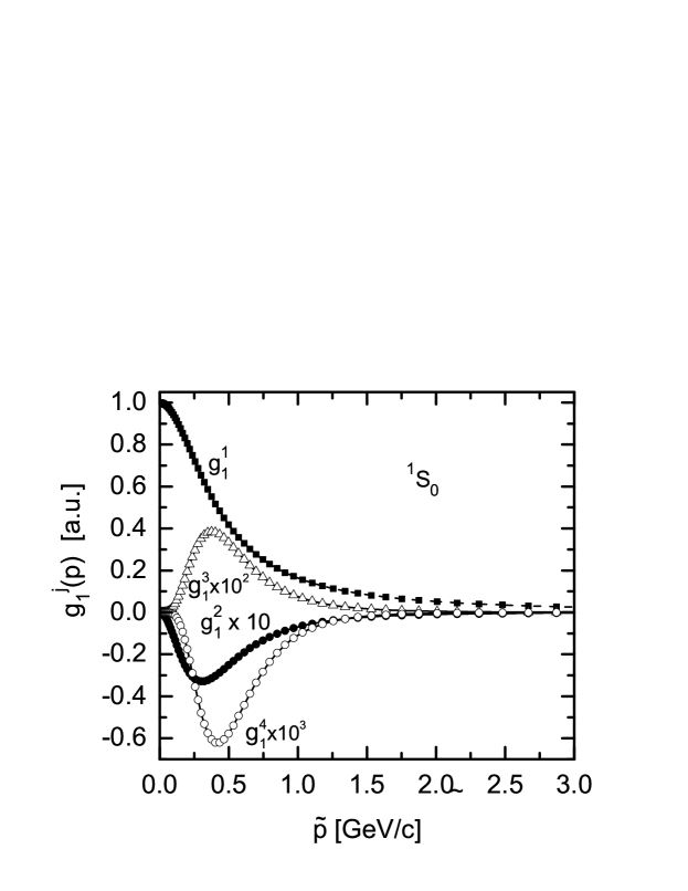
To display the behavior of the components of the vertex function, in Fig. 1 we present the resulting coefficients for the channel , , eq. (54), at for , and . It can be seen that at large these functions decrease as inverse powers of which permits to cast the approximate solution into the form
| (80) |
where the parameters and can be found from an analysis of the adjustment of eq. (80) to the approximate solution (see Table 11). The solid lines in Fig. 1 reflect the result of the fit of the numerical solution by eq. (80). The accuracy of the results implies that in such a way one can find solutions of the corresponding system of equations as continuous functions of which are extremely useful in practical applications. Similar analysis of other coefficient functions shows that an excellent fit of the numerical solutions can be achieved for all the partial components . From this encouraging result we argue that this method using hyperspherical harmonics can be considered as a reliable tool to solve the Bethe-Salpeter equation numerically, even with different parameterizations of the solution than the simple form (80). Unfortunately, for small meson masses the method becomes less effective, having a poor or even failing convergence feature and hence becomes less adequate, requiring a separate analysis (see also Ref. fb-tjon ).
Also, as mentioned above, at large values of the coupling constants , close to or even larger than the critical value , the numerical solutions become strongly dependent on , and which is a clear signal that (in absence of the cut-off form factors (16)) the solution becomes unstable at and disappears at . Such a situation is illustrated in Fig. 2 where we present the dependence of the mass on the values of the cut-off parameter at different coupling constants , below and above the critical value . It is seen that if the solution exists and is stable () then the mass is almost independent on the cut-off form factor and tends to a constant value at large . Contrarily, the dependence of the mass on at evidently indicates that in this case the solution becomes unstable and at large values of , , it can disappear at all. Such a behavior of the solution at exactly reproduces the peculiarities of the well-known collapse phenomenon for potentials like in nonrelativistic quantum mechanics (see, also discussions in Ref. karm2 ). In Fig. 3 the numerical solutions for the partial components are given for two values of the coupling constant, below (solid lines) and above the critical (dashed lines). In order to ensure the existence of the solution, calculations have been performed at a finite, however large, value of the cut-off parameter . It is seen that in the case of the asymptotic decrease of the wave functions is rather weak which implies the instability of the solution. In Fig. 3 the continuous lines reflect the result of a fit by eq. (80) which for the asymptotic region of the component , can be written in a simple form
| (81) |
where () and (). A comparison with eqs. (72) and (75) shows that for coupling constants below the critical value, , one has , while above , , i.e., the integral (70) without form factors (16) diverges. A similar behavior of the numerical solution occurs in the - channel as well (see, Fig. 4).
IV.3 Scalar coupling
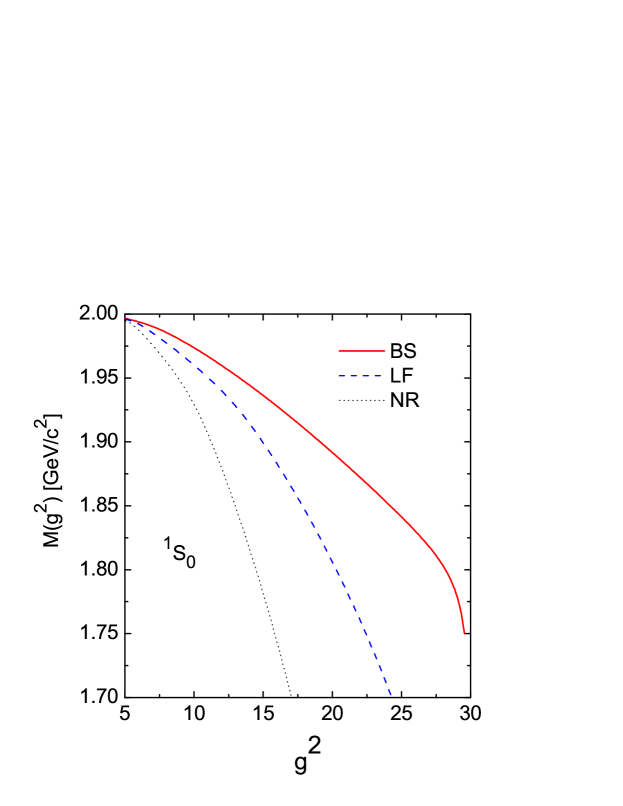
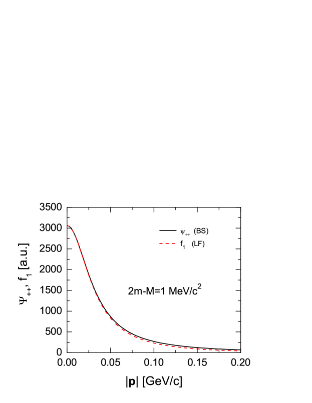
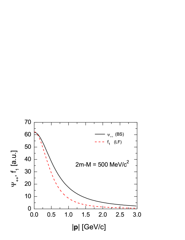
Having established the main features of the numerical procedure, we solve the BS equation within the hyperspherical harmonics method for different kinds of the exchanged mesons, i.e. scalar, pseudoscalar and vector mesons. We investigate the dependence of the bound state mass on the coupling constant and study the partial components as a function of the hypervariable at fixed values of and the coupling constant . All calculations have been done with and without the cut-off form factors (16) and, obviously, for the coupling constants below their critical values. We compare our results with other calculations performed for similar conditions, namely we widely compare our analysis to the ones obtained by Light Front (LF) dynamics karmanov and by the non relativistic (NR) Schrödinger approach. Note that within these approaches the dynamical variables used differ slightly from the ones used in BS formalism, hence a direct comparison of the calculated quantities is hampered. However, one can reconcile approaches by choosing one variable within the BS formalism, e.g. the modulus of the 3-dimensional relative momentum , and relate the corresponding quantities in LF or NR approaches through this variable for further comparisons.
Such relations have been found and reported in detail in Refs. our-BS-LF ; karmanov_PR . Here we note only that in determining relations between the BS and LF amplitudes one finds that in the channel only two components ( and ) of the BS amplitude correspond pairwise to the two LF functions and (notation as in Ref. karmanov ). The other BS components, when being projected on to the LF surface, vanish. Similarly, in the channel only five BS components survive on to LF surface our-BS-LF ; karmanov_PR . In Fig. 5 the mass of the bound state as a function of the coupling constant for scalar meson exchange is shown. The solid line corresponds to results within the BS approach, while the dashed and dotted lines show calculations with LF karmanov and NR (with an Yukawa-type potential) approaches, respectively. Only at low values of the binding energy different approaches provide similar results. As the coupling constant increases (increase of the binding energy) the difference becomes more and more significant. Even within two relativistic frameworks, BS and LF formalisms, the difference increases with the binding energy increase. This is illustrated also in Figs. 6 and 7 where the wave function , eq. (46), is compared to the corresponding LF wave function karmanov for two different binding energies. It is seen that the two approaches provide similar results for low, and rather different results for high values of the binding energy. Obviously, this is a direct consequence of the different treatment of the relativistic effects within the BS and LF formalisms. Since when projecting the BS amplitude on to the LF surface, some partial components (with negative -spins) vanish, the observed large difference between BS and LF results serves as a hint that in this case the role of the components with negative -spins increases. This can be checked by computing the pseudo probabilities for different components, eq. (50), at several values of the binding energy. To this end, we apply the transformation eq. (25) (or eq. (45) for the state) to the set of functions , preliminarily obtained numerically from the series (54)-(56) (or (57)-(60)). The corresponding results for the channel are collected in Table 12, where the pseudo probabilities for different components have been computed assuming the total normalization to be
| (82) |
As expected, the contribution of the component is negligibly small for weakly bound systems and significant for large binding energies. Similar conclusions hold for the – state as well. As mentioned, the BS system of equations for the partial components have been solved for a coupling constant below the critical value. However, there is also a lower limit below which the solution of the BS equation disappears, in a fully analogy with the nonrelativistic Schrödinger equation, when, for shallow potentials, bound states do not exist. Another observation is the result that the condition provides an equation for which in the interval can have more than one solution. In such a case the lowest value of corresponds to the ground state, while others refer to the discrete excited state of the system. We investigated also the behaviour of the partial vertex functions for the excited states and found that, likewise in the nonrelativistic case, these functions possess zeros as functions of . This is in a good agreement with our previous results obtained for the two-dimensional mesh nash_yaf1 .
IV.4 Pseudoscalar meson exchange
As follows from eq. (51), the system of equations for pseudoscalar meson exchange is quite similar to the previously described scalar case (see also Tables 4-6). However, contrary to the scalar case, when the main components and in eqs. (61) and (64) are determined by pure attractive kernels, for the pseudoscalar exchange one of these components is governed by a pure repulsive kernel (c.f. Tables 2 and 3). Thus, the resulting balance of forces forming the bound state for pseudoscalar exchange is more sophisticated. As a consequence, to ensure an attractive residual kernel for creation of a given bound state , the BS equation requires larger values of the coupling constant . Consequently, this can lead to subtle situations when the minimal value of is close to or even above the critical value , which may cause problems with the stability of the solution. Namely such a situation we encountered in our numerical calculations for a two-nucleon like system with pseudoscalar exchanges for which the stable bound state (without cutoff form factors) does not exist at all. Similar result has been obtained also within the LF approach karmanov and seems to be of a general nature, i.e. there is no relativistic bound state in a deuteron-like system with pure pseudoscalar exchange.
Another striking feature here is connected to the behavior of the binding energy as a function of the coupling constant. In Fig. 8, the dependencies of the binding energy for the state are shown for some values of the cutoff parameter . It is clear that such a dependence is very sharp – binding energy increases very rapidly with , which is in agreement with the results reported in Ref. karmanov .
IV.5 Vector meson exchange
Since the contribution of vector meson exchange in the nucleon-nucleon potential is repulsive a deuteron-like bound state cannot be formed by pure vector meson exchanges, therefore an investigation of the homogeneous BS equation with such kernels is hampered. However, one can consider a different two-fermion system such as the electron-positron pair, for which the vector exchange potential does have a bound state. Note that the general form of the BS equation, eq. (11), in the particle-antiparticle channel is maintained almost unchanged (see, e.g. Refs. nakan and itz ) so that a relativistic description of the positronium can be achieved by eq. (11) with , and . Unfortunately, the knowledge of the positronium, as a two-fermion bound system, is rather scarce positr , even the absolute value of the binding energy is not definitely established.
Nowadays only the transition energy between different positronium levels (e.g., between para- and ortho-positronium) is an object of experimental and theoretical investigation positr . Compared to the electron mass this quantity is very small LL , being of the order (where is the fine structure constant, is the electron mass and is the positronium binding energy predicted by the nonrelativistic Schrödinger equation). Consequently, the procedure of solving the BS equation numerically for the bound state and calculations of the transition energy and comparison with experimental data require extremely high accuracy of calculations and large computational resources. Moreover, as mentioned before, in case of vanishing masses of the exchange particle, the convergence of the method is rather ill defined and the implementation of cut-off form factors becomes a necessity in numerical calculations. Therefore, in analyzing effects of relativistic corrections computed within different schemes (e.g., within perturbative quantum electro-dynamics (QED), LF dynamics and BS formalism) one usually solves the corresponding equation with cut-off form factors and at an effective coupling constant much larger than the fine structure constant (see Ref. karmanov ) and compares the obtained results with those known analytically from the nonrelativistic Schrödinger equation. For this reason, a commonly accepted value of is , which corresponds to and to a nonrelativistic binding energy karmanov . In our calculations we also adopted such a coupling constant for which the para- and ortho- positronium binding energy has been calculated. The results are presented in Table 13, where the cut-off parameter and binding energies are given in units of the electron mass . The obtained results demonstrate that at large enough values of , the solution of the BS equation is quite stable and almost independent on . It is also seen that the BS equation provides a binding energy almost twice smaller than the nonrelativistic one which implies that the relativistic corrections are of repulsive nature. Analogous result has been obtained within the LF dynamics for the positronium karm2 . However, calculations within the perturbative QED show that the first order relativistic corrections are attractive. This contradictory result can serve as an indication that the adopted interaction kernel is not accurate enough for a refined description of the positronium within the ladder approximation. Other channels (e.g, the electron-positron annihilation itz ) and/or terms beyond the ladder approximation should be included into the analysis.
V Conclusion
We generalize a method based on hyperspherical harmonics to solve the homogeneous spinor-spinor Bethe-Salpeter equation in Euclidean space. To do so, we introduce a new basis of spin-angular harmonics, suitable to expand the Bethe-Salpeter vertex into four-dimensional hyperspherical harmonics. We obtain an explicit form of the corresponding system of one-dimensional integral equations for the partial components and formulate a proper numerical algorithm to solve this system of equations. The BS vertex functions are studied in detail for the and bound states with scalar, pseudoscalar and vector meson exchanges. Our results are in a good agreement with calculations within the non relativistic and Light Front Dynamics approaches.
Within the novel method the effectiveness of the numerical procedure is analyzed for the scalar, pseudoscalar and vector meson exchanges and conditions for stability of the solution are established. It is demonstrated that above some critical values of the coupling constant the solution of the BS equation does not exist unless the cut-off form factors are considered.
An advantage of the method is the possibility to present the numerical solution in a reliable and simple analytical parameterized form, extremely convenient in practical calculations of matrix elements within the BS formalism and for analytical continuation of the solution back to Minkowski space.
The method allows us to describe, in a covariant way, realistic two-body systems, such as the deuteron, the positronium and the variety of known mesons, as bound states of quark-antiquark pairs and to solve the inhomogeneous BS equation for scattering states in the continuum.
VI Acknowledgments
We thank V.A. Karmanov, G.V. Efimov and T. Frederico for valuable discussions and M. Mangin-Brinet for sending of results within Light Front calculating. S.M.D. and S.S.S. acknowledge the warm hospitality at the Elementary Particle Physics group, University of Rostock, where a bulk of this work was performed. This work was supported in part by the Heisenberg - Landau program of the JINR - FRG collaboration and by the Deutscher Akademischer Austauschdienst.
Appendix A Partial kernels
Here we present the explicit form of the kernels which determine the partial kernels and , eqs. (61)-(63) and (64)-(66). For this let us introduce an auxiliary quantity defined as
| (83) | |||||
where max (min) is the maximum (minimum) index of , and stand for the Gegenbauer polynomials and Legendre functions of the second kind, respectively, of imaginary argument with
Note that, as follows from properties of Gegenbauer polynomials, the quantities are different from zero for nonnegative and integer. The Legendre functions in eq. (83) for explicitly read as
By using the recurrent relations for the Gegenbauer polynomials batman , the partial kernels can be expressed via as
References
- (1) G. Rupp and J.A. Tjon, Phys. Rev. C45 (1992) 2133.
- (2) J. Fleischer, J.A. Tjon, Nucl. Phys. B84 (1975) 375.
- (3) M.J. Zuilhof, J.A. Tjon, Phys. Rev. C22 (1980) 2369 and references therein.
- (4) A.Yu. Umnikov, L.P. Kaptari, F.C Khanna, Phys. Rev. C56 (1997) 1700.
- (5) A. Holl, A. Krassnigg, P. Maris, C.D. Roberts, S.V. Wright, Phys. Rev. C71 (2005) 065204.
- (6) F. Gross, J.W. Van Orden, K. Holinde, Phys. Rev. C45 (1992) 2094.
- (7) I.V. Puzynin et al., Phys. Part. Nucl. 30 (1999) 87.
- (8) M. Mangin-Brinet, J. Carbonell, V.A. Karmanov, Phys. Rev. C68 (2003) 055203.
- (9) T. Frederico, J.H.O. Sales, B.V. Carlson, P.U. Sauer, Few Body Syst. 33 (2003) 89.
- (10) G.V. Efimov, Few-Body Syst. 33 (2003) 199.
- (11) B.L.G. Bakker, M. van Iersel, F. Pijlman, Few Body Syst. 33 (2003) 27.
- (12) R. Gilman, F. Gross, J. Phys. G28 (2002) R37.
- (13) L.P. Kaptari, A.Yu. Umnikov, S.G. Bondarenko, K.Yu. Kazakov, F.C. Khanna, B. Kämpfer, Phys. Rev. C54 (1996) 986.
- (14) L.P. Kaptari, B. Kaempfer, S.M. Dorkin, S.S. Semikh, Phys. Rev. C57 (1998) 1097.
- (15) L.P. Kaptari, B. Kämpfer, S.S. Semikh, S.M. Dorkin, Eur. Phys. J. A17 (2003) 119.
- (16) L.P. Kaptari, B. Kämpfer, S.S. Semikh, S.M. Dorkin, Eur. Phys. J. A19 (2004) 301.
- (17) D. Abbott et al., Phys. Rev. Lett. 84 (2000) 5053.
- (18) V. Komarov et al., Phys. Lett. B 553 (2003) 179.
-
(19)
D.M. Nikolenko et al., Nucl. Phys. A 684 (2001) 525c;
D. Abbott et al., Phys. Rev. Lett. 84 (2000) 5053. - (20) S.G. Karshenboim, Int. J. Mod. Phys. A19 (2004) 3879.
- (21) L.D. Landau, E.M. Lifshits, ”Quantum Electrodynamics”, Pergamon Press, 1965.
- (22) S.G. Bondarenko, V.V. Burov, M. Beyer, S.M. Dorkin, Phys. Rev. C58 (1998) 3143.
- (23) E.E. Salpeter and H.A. Bethe, Phys. Rev. 84 (1951) 1232.
- (24) J. Carbonell, B. Desplanques, V.A. Karmanov, J.-F. Mathiot, Phys. Rept. 300 (1998) 215.
- (25) C. Ciofi degli Atti, L.P. Kaptari, e-Print Archive: nucl-th/0407024; C. Ciofi degli Atti, L.P. Kaptari, D. Treleani, Phys. Rev. C63 (2001) 044601.01; S.G. Bondarenko, V.V. Burov, M. Beyer, S.M. Dorkin, e-Print Archive: nucl-th/9612047.
- (26) J.J. Kubis, Phys. Rev D6 (1972) 547.
- (27) T. Nieuwenhuis, J.A. Tjon, Few-Body Syst. 21 (1996) 167.
- (28) M. Mangin-Brinet, J. Carbonell, V.A. Karmanov, Phys. Rev. D64 (2001) 125005.
-
(29)
F.M. Lev, E. Pace, G. Salme, Phys. Rev. C62 (2000) 064004;
F.M. Lev, E. Pace, G. Salme, Phys. Rev. Lett. 83 (1999) 5250;
J.P.B.C. de Melo, T. Frederico, E. Pace, G. Salme, Phys. Lett. B581(2004) 75. - (30) S.S. Semikh, S.M. Dorkin, M. Beyer, L.P. Kaptari, Phys. Atom. Nucl. 68 (2005) 2022; Yad. Fiz. 68 (2005) 2084.
- (31) S.S. Semikh, S.M. Dorkin, M. Beyer, L.P. Kaptari, e-Print Archive: nucl-th/0410076.
- (32) N. Nakanishi, Prog. Theor. Phys. Suppl. 43 (1969) 1.
- (33) S.M. Dorkin, L.P. Kaptari, S.S. Semikh, Phys. Atom. Nucl. 60 (1997) 1629; Yad. Fiz. 60 (1997) 1784.
- (34) M.J. Levine, J. Wright, J.A. Tjon, Phys. Rev. 154 (1967) 1433; M. Fortes, A.D. Jackson, Nucl. Phys. A 175 (1971) 449.
- (35) G. Rupp, J.A. Tjon, Phys. Rev. C41 (1990) 472.
- (36) G.C. Wick, Phys. Rev. 96, 1124 (1954).
- (37) St. Glazek et al., Phys Rev. D47 (1993) 1599: St. Glazek, K. Wilson, Phys. Rev. D47 (1993) 4657.
- (38) G.E. Forsythe, M.A. Malcolm, C.B. Moler, Computer Methods for Mathematical Computations (Prentice-Hall, Englewood Cliffs, N.J., 1977).
- (39) A. Erdelyi, Higher Transcendental Functions (Bateman Manuscript Project), Ed. by A. Erdelyi, (McGraw-Hill, New York, 1953), Vol. 2.
- (40) S.G. Bondarenko, V.V. Burov, M. Beyer, S.M. Dorkin, Few Body Syst., 26 (1999) 185.
- (41) C. Itzykson, J.-B. Zuber. Quantum Field Theory, McGraw-Hill, 1980.