Self-Trapping of Bose-Einstein Condensates in an Optical Lattice: the Effect of the System Dimension

Abstract

In the present paper, we investigate the dynamics of a Bose-Einstein condensates (BEC) loaded into an deep optical lattice of 1D, 2D and 3D, both analytically and numerically. We focus on the self-trapping state and the effect of the system dimension. Under the tight-binding approximation we obtain an analytical criterion for the self-trapping state of BEC using time-dependent variational method. The phase diagram for self-trapping, soliton, breather, or diffusion of the BEC cloud is obtained accordingly and verified by directly solving the discrete Gross-Pitaevskii equation (GPE) numerically. In particular, we find that the criterion and the phase diagrams are modified dramatically by the dimension of the lattices.

I Introduction

Recently, the Bose-Einstein condensates (BECs) in an optical lattice attract much attention both experimentally and theoreticallyrev1 . This is partly because the physical parameters, e.g., lattice parameters, interaction strength, etc., in such a clean system (”clean” means perfect periodicity without impurity) can be manipulated at will using modern experimental technique like Feshbach resonance. Taking this advantage people have observed well-known and long-predicted phenomena, such as Bloch oscillationsd1 and the quantum phase transition between superfluid and Mott insulatord2 . More importantly, there are new phenomena that have been either observed or predicted in this system, for example, nonlinear Landau-Zener tunneling between Bloch bandsd3 ; d4 and the strongly inhibited transport of one-dimensional BEC in an optical latticed5 .

Another intriguing phenomenon, namely, self-trapping, was recently observed experimentally in this system c10 . In such a experiment, it was observed that a BEC cloud with repulsive interaction initially loaded in an optical lattice was self-trapped or localized and the diffusion was completely blocked when the number of the degenerate bosonic atom was larger than a critical value. This is quite counterintuitive. Even without interaction, a wave packet with a narrow distribution in the Brillouin zone expands continuously inside a periodic potential. When there is an interaction between atoms and it is repulsive, one would certainly expect the wave packet to expand. On the other aspect, the self-trapping phenomenon also attract many theoretical efforts and a lot of meaningful results have been obtainedc11 ; c12 ; c13 ; c14 ; c15 ; kivshar ; c16 . However, most of these analyses are limited to 1D system. Beyond these 1D approximation, the localized statesc17 -c18 , self-trapping and other quantum phenomenac19 -c22 have been observed in high-dimensional optical lattices. To our knowledge, however, there are no systematical theoretical analyses on the dynamics of BEC loaded into multi-dimensional optical lattices. There leaves some important problems, e.g., what is the effect of the system dimension on the dynamics of BEC in optical lattices ?

In this paper, we address this issue both analytically and numerically focusing on the intriguing self-trapping phenomenon, within the tight-binding approximation. Based on the discrete GPE and exploiting a time-dependent variational approach, we obtain an analytical criterion for the self-trapping state of BEC and the phase diagram for self-trapping, soliton, breather, or diffusion of the BEC cloud. Our results show that, the change on the dimension of the system leads to many interesting consequence: i) Self-trapping state can also emerge in higher-dimension systems, however, compared to the 1D situation its parameter domain in the phase diagram is largely shrunken; ii) The stable moving soliton and breather solutions of the wavepackets that exist in $1D$ system, no longer stand in $2D$ and $3D$ systems. iii) In addition, when the self-trapping occurs, the ratio between the final BEC cloud width and the initial wavepacket width is greatly modified in $2D$ and $3D$ systems compared to the 1D case.

Our paper is organized as follows. In Sec.II, under the tight-binding approximation, we obtain a discrete GPE that governs the dynamical behavior of BEC in deep $3D$ periodic optical lattices. In Sec.III, using the time-dependent variation of a Gaussian profile wavepacket, the dynamics of BEC is discussed analytically and the critical conditions for occurrence of self-trapping state are obtained. Moreover, the phase diagram for self-trapping, soliton, breather, or diffusion of the BEC matter waves is obtained accordingly. In Sec.IV, directly solving GPE is exploited to confirm our theoretical predictions. Sec.V, are our discussion and conclusion.

II NONLINEAR DISCRETE MODEL

We focus our attention on the situation that a BEC is loaded into a $3D$ optical lattices. In the mean field approximation, the $3D$ BEC dynamics at T=0 satisfies the GPE

$$i\hslash\frac{\partial\Psi}{\partial t}=-\frac{\hslash^{2}}{2M}\nabla^{2}\Psi+(V_{opt}(\overrightarrow{r})+\frac{4\pi\hslash^{2}a_{s}}{M}|\Psi|^{2})\Psi$$ (1)

where $\Psi$ is the wave function of the condensate. The coupling constant $4\pi\hslash^{2}a_{s}/M$, which relate to the mass of the atoms $M$ and the repulsive (attraction) s-wave scattering length $a_{s}>0(a_{s}<0)$, is the nonlinear coefficient corresponding to the two body interactions, $V_{opt}(\overrightarrow{r})=V_{\max}(\cos(2\kappa x)+$ $\cos(2\kappa y)+\cos(2\kappa z))$ is the external optical potential created by three orthogonal pairs of counter-propagating laser beamsc23 , $\kappa$ is the wave number of the laser lights that generate the optical lattice.
All the variables can be re-scaled to be dimensionless by the system’s basic parameters $t$ $\sim$ $t\nu$, $x$ $\sim$ $\kappa x$, $\Psi\sim$ $\frac{1}{\sqrt{\kappa N}}\Psi$, then GPE (1) becomes

$$i\frac{\partial\Psi}{\partial t}=-\nabla^{2}\Psi+V(\overrightarrow{r})\Psi+\frac{4\pi\hslash^{2}a_{s}\kappa N}{M\hslash\nu}|\Psi|^{2}\Psi$$ (2)

where $N$ is the total number of atoms, $V(\overrightarrow{r})=V_{0}[\cos(2x)+$ $\cos(2y)+\cos(2z)]$, the parameter $V_{0}=V_{\max}/2E_{R}$ is the strength of the optical lattices, with $E_{R}=\hslash^{2}\kappa^{2}/2M$ is the recoil energy of the lattice, $\nu=E_{R}/\hslash$. The associated Hamiltonian is

$$H=\int d\overrightarrow{r}[-\Psi(\overrightarrow{\nabla}\Psi)\Psi^{\ast}+V(\overrightarrow{r})|\Psi|^{2}+\frac{2\pi\hslash^{2}a_{s}\kappa N}{M\hslash\nu}|\Psi|^{4}]$$ (3)

In order to understand the dynamical behaviors of BEC in deep 3D optical lattices, it is worthwhile to study the system in certain extreme limits. The particular limit that we now insight into is the tight-binding approximation, where the lattice is so strong that the BEC system can be looked as a chain of trapped BECs that are weakly linkedc11 . Under the tight binding limit, the condensate parameter can be written as

$$\Psi(\overrightarrow{r},t)=\sum_{n,m,k}\psi_{n,m,k}(t)\phi(\overrightarrow{r}-\overrightarrow{r}_{n,m,k})$$ (4)

where $\psi_{n,m,k}(t)=\sqrt{N_{n,m,k}(t)}e^{i\theta_{n,m,k}(t)}$ is the ($n,m,k)$th amplitude, $N_{n,m,k}$ and $\theta_{n,m,k}(t)$ are the number of particles and phases in the well $(n,m,k)$. $\sum_{n,m,k}|\Psi_{n,m,k}|^{2}=1$, $\phi(\overrightarrow{r}-\overrightarrow{r}_{n,m,k})$ is the condensate wavefunction localized in the well $(n,m,k)$, with the normalization $\int d\overrightarrow{r}\phi_{n,m,k}^{2}=1$, and the orthogonality of the condensate wave functions $\int d\overrightarrow{r}\phi_{n,m,k}\phi_{n+1,m,k}\simeq 0,\int d\overrightarrow{r}\phi_{n,m,k}\phi_{n,m+1,k}\simeq 0,\int d\overrightarrow{r}\phi_{n,m,k}\phi_{n,m,k+1}\simeq 0$. Inserting the nonlinear tight-binding approximation (4) into the GPE (2) and integrating out the spatial degrees of freedom, following re-scale the time as $t\rightarrow 2Kt$, we find the reduced GPE

$$i\frac{\partial\psi_{n,m,k}}{\partial t} = -\frac{1}{2}(\psi_{n-1,m,k}+\psi_{n+1,m,k}+\psi_{n,m-1,k}$$ (5)

$$+\psi_{n,m+1,k}+\psi_{n,m,k-1}+\psi_{n,m,k+1})$$

$$+(A+\Lambda|\psi_{n,m,k}|^{2})\psi_{n,m,k}$$

where $A=\frac{1}{2K}\int d\overrightarrow{r}[(\nabla\phi_{n,m,k})^{2}+V(\overrightarrow{r})\phi_{n,m,k}{}^{2}]$, $\Lambda=\frac{1}{2K}\frac{4\pi\hslash^{2}a_{s}\kappa N}{M\hslash\nu}\int d\overrightarrow{r}\phi_{n,m,k}{}^{4}$ is the ratio of the nonlinear coefficient, induced by the two-body interatomic interactions. And the included parameter $K\simeq-\int dr\{(\nabla\phi_{n+1,m,k}\nabla\phi_{n,m,k}+\nabla\phi_{n,m+1,k}\nabla\phi_{n,m,k}+\nabla\phi_{n,m,k+1}\nabla\phi_{n,m,k})+V_{0}[\cos(2x)\phi_{n+1,m,k}\phi_{n,m,k}+\cos(2y)\phi_{n,m+1,k}\phi_{n,m,k}+\cos(2z)\phi_{n,m,k+1}\phi_{n,m,k}]\}$ is the tunneling rates between the adjacent sites $(n,m,k)$ and $(n+1,m+1,k+1)$. In order to make an agreement with the experiments done with ${}^{87}Rb$, the two-body interaction term is expected to be positive, that is $\Lambda>0$.

Equation (5) can be written as $\overset{\cdot}{\psi}_{n,m,k}=\partial H/\partial(i\psi_{n,m,k}^{\ast})$, where $H$ is the Hamiltonian function

$$H = \sum_{n,m,k}[-\frac{1}{2}(\psi_{n,m,k}\psi_{n+1,m,k}^{\ast}+\psi_{n,m,k}^{\ast}\psi_{n+1,m,k}$$ (6)

$$+\psi_{n,m,k}\psi_{n,m+1,k}^{\ast}+\psi_{n,m,k}^{\ast}\psi_{n,m+1,k}$$

$$+\psi_{n,m,k}\psi_{n,m,k+1}^{\ast}+\psi_{n,m,k}^{\ast}\psi_{n,m,k+1})$$

$$+A|\psi_{n,m,k}|^{2}+\frac{\Lambda}{2}|\psi_{n,m,k}|^{4}]$$

III ANALYTIC RESULTS BASED ON THE TIME-DEPENDENT VARIATIONAL APPROACH

To study the dynamics of the BEC wavepacket loaded into multi-dimensional optical lattices, we consider the evolution of a Gaussian profile wavepacket, which we parametrize as $\psi_{n,m,k}(t)=\sqrt{\rho}\exp\{-\frac{(n-\xi_{x})^{2}}{R_{x}^{2}}-\frac{(m-\xi_{y})^{2}}{R_{y}^{2}}-\frac{(k-\xi_{z})^{2}}{R_{z}^{2}}+i[p_{x}(n-\xi_{x})+p_{y}(m-\xi_{y})+p_{z}(k-\xi_{z})]+\frac{i}{2}[\delta_{x}(n-\xi_{x})^{2}+\delta_{y}(m-\xi_{y})^{2}+\delta_{z}(k-\xi_{z})^{2}\}$, define $\alpha=x,y$ or $z$, where $\xi_{\alpha}(t)$ and $R_{\alpha}(t)$ are the center and the width of the wavepacket in the $\alpha$ direction, $p_{\alpha}(t)$ and $\delta_{\alpha}(t)$ are their associated momenta in the $\alpha$ direction, and $\rho$ is a normalization factor. The wavepacket dynamical evolution can be obtained by a variational principle from the Lagrangian $L=\sum_{n,m,k}i(\overset{\cdot}{\psi}_{n,m,k}\psi_{n,m,k}^{\ast}-\psi_{n,m,k}^{\ast}\overset{\cdot}{\psi}_{n,m,k}^{\ast})-H$, with the equations of motion for the variational parameters $q_{i}(t)=$ $\xi_{\alpha},R_{\alpha},p_{\alpha},\delta_{\alpha}$ given by $\frac{d}{dt}\frac{\partial L}{\partial\overset{\cdot}{q_{i}}}=\frac{\partial L}{\partial q_{i}}$, where $H$ is given by Eq.(6). In calculation, we can replace the sums over $(n,m,k)$ in the Lagrangian with integrals when $R_{\alpha}$ is not too smallc11 . In this limit, the normalization factor is obtained as $\rho=\frac{1}{\sqrt{\pi/2}^{3}\underset{\alpha=x,y,z}{\prod}R_{\alpha}}$ from $\int_{-\infty}^{\infty}\int_{-\infty}^{\infty}\int_{-\infty}^{\infty}|\psi_{n,m,k}|^{2}dndmdk=1$. All these parameters lead to $L=-V(R_{{}_{\alpha}},\xi_{{}_{\alpha}})-\frac{\Lambda}{2\sqrt{\pi}^{3}\underset{\beta=x,y,z}{\prod}R_{\beta}}+\sum_{{}_{{}_{\alpha}}}(2p_{{}_{\alpha}}\overset{\cdot}{\xi}_{{}_{\alpha}}-\frac{1}{4}\overset{\cdot}{\delta}_{{}_{\alpha}}R_{{}_{\alpha}}^{2}+e^{-\sigma_{\alpha}}\cos p_{{}_{\alpha}})$, where $\sigma_{\alpha}=\frac{1}{2R_{\alpha}^{2}}+\frac{R_{\alpha}^{2}\delta_{\alpha}^{2}}{8}$, and $V(R_{{}_{\alpha}},\xi_{{}_{\alpha}})=\rho\int_{-\infty}^{\infty}\int_{-\infty}^{\infty}\int_{-\infty}^{\infty}dndmdkAe^{-(\frac{2(n-\xi_{x})^{2}}{R_{x}^{2}}+\frac{2(m-\xi_{y})^{2}}{R_{y}^{2}}+\frac{2(k-\xi_{z})^{2}}{R_{z}^{2}})}$. The equations of motion of collective variables $\xi_{\alpha}(t),$ $R_{\alpha}(t),$ $p_{\alpha}(t),$ $\delta_{\alpha}(t)$ are given by

$$\overset{\cdot}{p_{\alpha}} = -\frac{1}{2}\frac{\partial V}{\partial\xi_{\alpha}}$$

$$\overset{\cdot}{\xi_{\alpha}} = \frac{1}{2}e^{-\sigma_{\alpha}}\sin p_{\alpha}$$

$$\overset{\cdot}{\delta_{\alpha}} = \cos p_{\alpha}(\frac{2}{R_{\alpha}^{4}}-\frac{\delta_{\alpha}^{2}}{2})e^{-\sigma_{\alpha}}-\frac{2}{R_{\alpha}}\frac{\partial V}{\partial R_{\alpha}}$$

$$+\frac{\Lambda}{\sqrt{\pi}^{3}R_{\alpha}^{3}\underset{\underset{(\beta\neq\alpha)}{\beta=x,y,z}}{\prod}R_{\beta}}$$

$$\overset{\cdot}{R_{\alpha}} = \frac{R_{\alpha}}{2}\delta_{\alpha}e^{-\sigma_{\alpha}}\cos p_{\alpha}$$ (7)

For simplicity, we assume: $\ R_{x}=R_{y}=R_{z}=R,$ $p_{x}=p_{y}=p_{z}=p,$ $\delta_{x}=\delta_{y}=\delta_{z}=\delta,$ $\sigma_{x}=\sigma_{y}=\sigma_{z}=\sigma=\frac{1}{2R^{2}}+\frac{R^{2}\delta^{2}}{8},$ $\xi_{x}=\xi_{y}=\xi_{z}=\xi.$ Then, the effective Hamiltonian reduce to

$$H=-De^{-\sigma}\cos p+V(R,\xi)+\frac{\Lambda}{2\sqrt{\pi}^{D}R^{D}}$$ (8)

where $D=1,2,$ or $3$ reflects the dimension of the system. It can be seen from Eq.(8), $D$ plays an important role in the effective Hamiltonian.

The group velocity of the wave packet is

$$v_{g}\equiv\frac{\partial H}{\partial p}=\overset{\cdot}{\xi}=\frac{\tan p}{m^{\ast}}$$ (9)

with the inverse effective mass

$$\frac{1}{m^{\ast}}\equiv\frac{\partial^{2}H}{\partial p^{2}}=\cos p\bullet e^{-\sigma}$$ (10)

It is important to note that, because this effective mass is related to the quasi-momentum, the system will exist rich dynamical phenomenons. Especially, when $\cos p<0$, the effective mass is negative and the system can exist the localized solution, i.e. soliton solution. For a untilted trap, $V(R,\xi)=0$, the momentum $p(t)$ remains a constant $p_{0}$. Initially, we set $\xi_{0}=0$ and $\delta_{0}=0$. In this case, the effective Hamiltonian becomes

$$H=-D\cos p_{0}\bullet e^{-\sigma}+\frac{\Lambda}{2\sqrt{\pi}^{D}R^{D}}$$ (11)

Clearly, the dynamical properties of the system not only governed by the parameter $\Lambda$, but also influenced by the dimension $D$. As discussed above, the dynamics of the wavepacket are modified significantly by the sign of $\cos p_{0}$. So two cases with $\cos p_{0}>0$ and $\cos p_{0}<0$ will be discussed respectively.

III.1 $\cos p_{0}>0$

Let us first consider the case with $\cos p_{0}>0$, following this case there exist two nonlinear phenomenons.

Self-trapping: Equation (9) shows that when the diverging effective mass $m^{\ast}\rightarrow\infty$, the group velocity of the wave packet $v_{g}\rightarrow 0$, this corresponding to a self-trapping solution. Thus, for $t\rightarrow\infty$ one has $R\rightarrow R_{\max}$, $\delta\rightarrow\infty$ and $\overset{\cdot}{\xi}\rightarrow 0,H\rightarrow\frac{\Lambda}{2\sqrt{\pi}^{D}R_{\max}^{D}}$.  Because the Hamiltonian is conserved, $H=H_{0}>0$, so when $H_{0}>0$, we get the maximum value of the width

$$R_{\max}=(\frac{\Lambda}{\frac{\Lambda}{R_{0}^{D}}-2D\sqrt{\pi}^{D}\cos p_{0}\bullet e^{-\frac{1}{2R_{0}^{2}}}})^{1/D}$$ (12)

Diffusion: In this case, for $t\rightarrow\infty$, one has $R\rightarrow\infty$, $\delta\rightarrow 0$ and $\overset{\cdot}{\xi}\rightarrow\frac{1}{2}\sin p_{0}$, as well as the effective Hamiltonian $H\rightarrow-D\cos p_{0}$. So the condition $-\cos p_{0}\leq$ $H_{0}\leq 0$ corresponding to the diffusive region of the system. The critical condition between self-trapping and diffusion is given by $H_{0}=0$, i.e., $-D\cos p_{0}\bullet e^{-\frac{1}{2R_{0}^{2}}}+\frac{\Lambda}{2\sqrt{\pi}^{D}R_{0}^{D}}=0$, one can get

$$\Lambda_{c}=2\sqrt{\pi}^{D}DR_{0}^{D}\cos p_{0}\bullet e^{-\frac{1}{2R_{0}^{2}}}$$ (13)

The self-trapping phenomenon occurs at $\Lambda>\Lambda_{c}$, and the diffusion occurs at $\Lambda<\Lambda_{c}$. By observing the equation (12), one readily obtain

$$R_{0}/R_{\max}=(1-\frac{\Lambda_{c}}{\Lambda})^{1/D}$$ (14)

It is clear that when D=1, Eqs. (13) and (14) reduce to the corresponding results given inc11 .

III.2 $\cos p_{0}<0$

When $\cos p_{0}<0$, the dynamics of the system (11) can be governed by (see Eq.(7)).

$$\overset{\cdot}{\delta} = -D|\cos p_{0}|(\frac{2}{R^{4}}-\frac{\delta^{2}}{2})e^{-\sigma}+\frac{\Lambda}{\sqrt{\pi}^{D}R^{D+2}}$$

$$\overset{\cdot}{R} = -\frac{R}{2}\delta e^{-\sigma}|\cos p_{0}|$$ (15)

This system has moving soliton solution. The moving soliton solution corresponding to the fixed points $\overset{\cdot}{R}=0$ and $\overset{\cdot}{\delta}=0$, $\overset{\cdot}{\xi}=$constant. One readily gets from (15):

$$\delta_{0}=0,\Lambda_{c}=2\sqrt{\pi}^{D}R_{0}^{D-2}|\cos p_{0}|e^{-\frac{1}{2R_{0}^{2}}}$$ (16)

We now discuss the stability of this soliton state. Let $\delta=\delta_{0}+\delta^{\prime},R=R_{0}+R^{\prime},$ and linearize Eq.(15) at the soliton state, we have:

$$\binom{\overset{\cdot}{\delta^{\prime}}}{\overset{\cdot}{R^{\prime}}}=\frac{\Lambda}{4\sqrt{\pi}^{D}R_{0}^{D+3}}\left(\begin{array}[]{cc}0&4(2-D-1/R_{0}^{2})\\ -R_{0}^{6}&0\end{array}\right)\binom{\delta^{\prime}}{R^{\prime}}$$ (17)

one obtains its eigenvalue $\lambda^{2}=\frac{1}{2}R_{0}^{3}(D-2+1/R_{0}^{2}).$ It is clear that when $D=1,$ the soliton state is a center point (note that $R_{0}>1$), stable soliton solution and breather solution can exist in $1D$ case. The dynamical behaviors of the wavepacket in $1D$ case is discussed in detail in Ref.c11 . When $D>1$, however, the soliton solution is a saddle point, no stable soliton and breather solutions can exist in the system. The numerical results for the phase diagram in the $R-\delta$ space given by Eq.(15) for $2D$ and $3D$ cases are shown in Fig.1. One can find that soliton and breather cannot exist in higher dimensional system. When $\Lambda>\Lambda_{c}$, for $t\rightarrow\infty,$ one has $R\rightarrow R_{\min}<R_{0}$ and $\delta\rightarrow\infty$. It means that the BEC wavepacket remains finite finally and the self-trapping phenomenon occurs. While $\Lambda<\Lambda_{c}$, the situation is changed. It is shown that $R\rightarrow\infty$ and $\delta\rightarrow 0$, diffusion takes place. That is, the dynamics of the BEC wavepackets in $1D$, $2D$ and $3D$ optical lattices are very different. In $1D$, soliton, breather, and self-trapping states can exist. In 2D and 3D systems, however, only self-trapping state can exist when $\Lambda>\Lambda_{c}$.

Figure 1: The Phase diagram of Eq. (15) for $2D$ [(a), $R_{0}=5$, $\delta_{0}=0$] and $3D$ case [(b), $R_{0}=10$, $\delta_{0}=0$]

In this case ($\cos p_{0}<0$), after the self-trapping occurs, $R\rightarrow R_{\min}<R_{0}$, $\delta\rightarrow\infty$ and $\overset{\cdot}{\xi}\rightarrow 0$, $H\rightarrow\frac{\Lambda}{2\sqrt{\pi}^{D}R_{\min}^{D}}$, one can get from $H_{0}=H=-D\cos p_{0}\bullet e^{-\frac{1}{2R_{0}^{2}}}+\frac{\Lambda}{2\sqrt{\pi}^{D}R_{0}^{D}}$

$$R_{0}/R_{\min}=(1+\frac{\Lambda^{\prime}}{\Lambda})^{1/D}$$ (18)

where $\Lambda^{\prime}=2\sqrt{\pi}^{D}DR_{0}^{D}|\cos p_{0}|e^{-\frac{1}{2R_{0}^{2}}}$, and $\Lambda>\Lambda_{c}$.

The first and second panels in Fig.2 show the analytical results for the dynamical diagram of the wavepacket in the $\cos p_{0}-\Lambda_{c}$ plane. It reveals that the dynamics of the system can be influenced dramatically by the dimension. Compared with the $1D$ case, the results are modified greatly in $2D$ and $3D$ systems. The region of the self-trapping decreases quickly with $D$, while the regions of the diffusion increases with $D$. We can clearly find that the soliton and breather solutions disappear in $2D$ and $3D$ systems. It is also shown that, the effect of $D$ on the regions of the self-trapping is more significant when the width of wavepacket is increased.

Figure 2: The critical value $\Lambda_{c}$ against $\cos p_{0}$ (the first two panels) and initial width $R_{0}$ (the third panel)

The critical value $\Lambda_{c}$ against the initial wavepacket width $R_{0}$ given by Eqs.(13) and (16) are also described in the third panel in Fig.2. It is clear that the variation of self-trapping region against $R_{0}$ is very different for $1D$, $2D$, and $3D$ cases, especially, for $\cos p_{0}<0$ case. When $\cos p_{0}<0$, $\Lambda_{c}$ reaches a maximum in the beginning and then decreases with increasing $R_{0}$ in $1D$. However, this relation is modified in $2D$, where $\Lambda_{c}$ increases with $R_{0}$ sharply when $R_{0}<3$ and finally $\Lambda_{c}$ remains an invariable value when $R_{0}>3$. Especially, $\Lambda_{c}$ increases with $R_{0}$ linearly in $3D$. Moreover, for a fixed $R_{0}$, $\Lambda_{c}$ in $3D$ case is several times, even one order of magnitude larger than that in $1D$ and $2D$. That is, if the initial wavepacket is given, the higher the dimension is, the greater the atomic interactions or atom number are needed in order to get into the self-trapping state. Thus it can be seen the dimension has significant effect on the critical condition for the occurrence of the self-trapping state.

Figure 3: The value of $R_{0}/R_{\max}$ for $\cos p_{0}>0$ (a) and the minimum value $R_{\min}$ against the initial width $R_{0}$ for $\cos p_{0}<0$ (b)

Fig.3(a) shows the ratio $R_{0}/R_{\max}$ versus ratio $\Lambda/\Lambda_{c}$ for $\cos p_{0}>0$. When the self-trapping occurs, one can find that the final wavepacket width $R_{\max}$ is larger than the initial wavepacket width $R_{0}$. For a fixed $\Lambda/\Lambda_{c}$, $R_{0}/R_{\max}$ increases with increasing $D$. It means that, when $\Lambda>\Lambda_{c}$, the BEC cloud can easily get into self-trapping state with little adjustment of the initial wavepacket for higher dimension case. In addition, it is clearly that $R_{0}/R_{\max}$ increases with $\Lambda/\Lambda_{c}$ and close to 1 eventually for $1D$, $2D$, and $3D$ cases. In other words, for sufficiently large $\Lambda$, the BEC cloud will quickly get into self-trapping state for all the case and the effect of dimension is weakened.

Fig.3(b) shows the minimum wavepacket width $R_{\min}$ against the initial wavepacket width $R_{0}$ for $\cos p_{0}<0$. As is expressed, $R_{\min}$ is always smaller than $R_{0}$. More interestingly, $R_{\min}$ increases with $R_{0}$ in $1D$ and $3D$, while $R_{\min}$ keeps a constant ($0.75$) and nearly independent with $R_{0}$. On the other hand, because the effect mass given by Eq.(10) is negative, the BEC cloud will finally squeeze into several lattice points for $1D$ and $3D$ case and about two lattice points for $2D$ case.

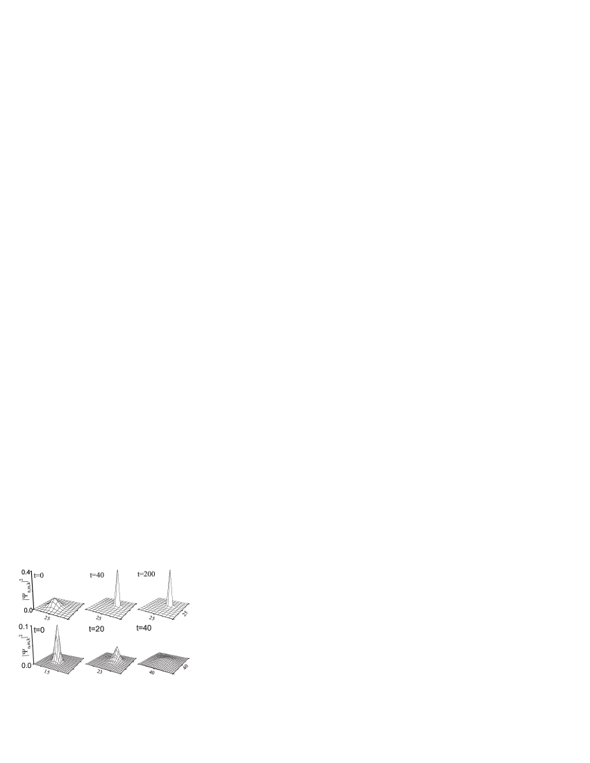
Figure 4: The dynamics of the $2D$ wavepacket with $\Lambda=6.5>\Lambda_{c}\simeq 4$ (the first panel) and $\Lambda=3.5<\Lambda_{c}\simeq 4$ (the second panel), $R_{0}=2.5$, $p_{0}=3\pi/4$

IV
NUMERICAL SIMULATIONS ON THE GPE

To confirm the above theoretical predictions, the direct numerical simulations of the full discrete GPE(5) are presented in Figs.4-9.

The numerical results for the dynamics of $2D$ wavepacket with small initial width ($R_{0}=2.5$) are provided in Fig.4. It is explicit that when $\Lambda>\Lambda_{c}$ (first panel) the BEC cloud is quickly squeezed into two optical lattices finally and the width of the wavepacket remains finite (self-trapping). On the contrary, when $\Lambda<\Lambda_{c}$ (second panel), as it is expected the wavepacket will expanding indefinitely with time (diffusion).

Figs.5-7 show the numerical results of the wavepacket with wider initial wavepacket ($R_{0}=10$). The results with $\Lambda=5>\Lambda_{c}\approx 4.4$ are shown in Fig.5. One can find that the wavepacket is also trapped into several lattices (at $t\approx 100$) as wavepacket moving. In this case, however, the self-trapping occurs only during a certain time ($t\lesssim 100$, this time scale decreasing with $\Lambda$) but then the wavepacket start to diffuse. If we strengthen the nonlinear term to $\Lambda=20>>\Lambda_{c}=4.4$, the associated results are shown in Fig.6. It indicates that the condensate is trapped almost in two optical lattices eventually and diffusion is not occur. Also, Fig.7 provides the results with $\Lambda<\Lambda_{c}$, as expected the diffusion result is obtained.

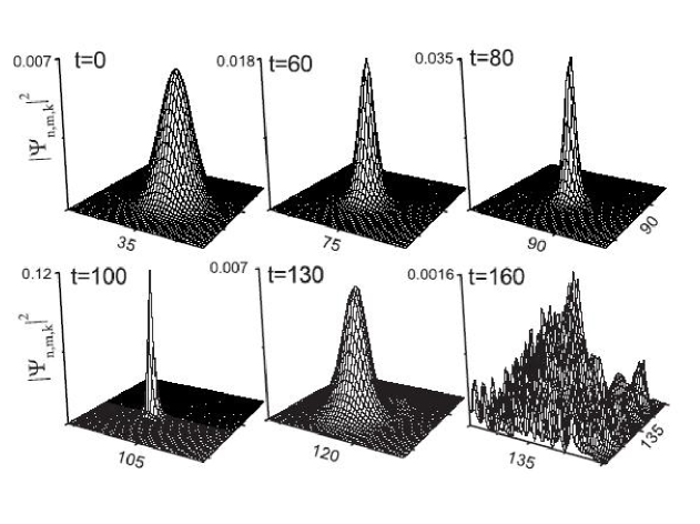
Figure 5: The dynamics of the $2D$ wavepacket with $\Lambda=5>\Lambda_{c}\simeq 4.4$, $R_{0}=10$, $p_{0}=3\pi/4$

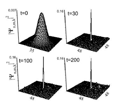
Figure 6: The dynamics of the $2D$ wavepacket with $\Lambda=20>>\Lambda_{c}\simeq 4.4$, $R_{0}=10$, $p_{0}=3\pi/4$

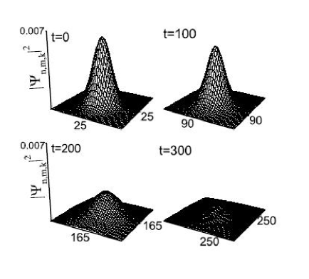
Figure 7: The dynamics of the $2D$ wavepacket with $\Lambda=3<\Lambda_{c}\simeq 4.4$, $R_{0}=10$, $p_{0}=3\pi/4$

Figs.8-9 show the numerical results for the dynamics of 3D wavepacket. Differ from the results in $2D$, when $\Lambda>\Lambda_{c}$ (the first panel in Fig.8 and Fig.9, respectively), the $3D$ wavepacket gets into self-trapping state and finally, the wavepacket splits into two pieces and localized state appears. The results with $\Lambda<\Lambda_{c}$ (the second panel in Fig.8 and Fig.9, respectively) give the diffusion results. It is clearly that the above numerical results are in good agreement with our variational predications. It can be seen the dimension of the lattices has significant effect on the dynamic of BEC wavepackets moving in optical lattices.

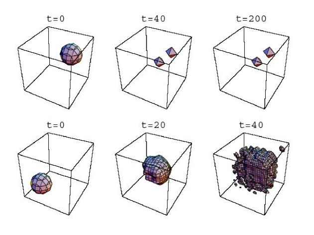
Figure 8: The dynamics of the $3D$ wavepacket with $\Lambda=30>\Lambda_{c}$ $\simeq 18$ (the first panel) and $\Lambda=15<\Lambda_{c}$ $\simeq 18$ (the second panel), $R_{0}=2.5$, $p_{0}=3\pi/4$

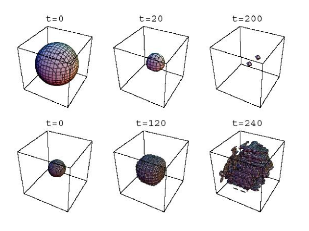
Figure 9: The dynamics of the $3D$ wavepacket with $\Lambda=90>\Lambda_{c}$ $\simeq 79$ (the first panel) and $\Lambda=50<\Lambda_{c}$ $\simeq 79$ (the second panel), $R_{0}=10$, $p_{0}=3\pi/4$

V
Conclusion

To summarize, we have investigated the dynamics of a BEC wavepacket loaded into a deep multi-dimensional periodic optical lattices both numerically and analytically, focusing on the effect of the lattice dimension. Our study shows that the dynamics of the BEC wavepacket is quite different in $1D$, $2D$ or $3D$ systems. For example, the stable moving soliton and breather states that exist in $1D$ lattice system no longer stand in $2D$ and $3D$ lattice systems. We also obtain an analytical criterion for the self-trapping state of BEC and phase diagram for self-trapping, soliton, breather, or diffusion of the BEC cloud for 1D, 2D and 3D, respectively. The above analytical results are confirmed by our directly solving the GPE. We hope that our studies will stimulate the experiments in the direction.

References

- (1) O. Morsch and M. Oberthaler, Rev. Mod. Phys. 78, 179 (2006), and references therein.
- (2) O. Morsch, J. H. Muller, M. Cristiani, D. Ciampini, and E. Arimondo, Phys. Rev. Lett. 87, 140402 (2001).
- (3) M. Greiner, O. Mandel, T. Esslinger, T. Hansch, and I. Bloch, Nature (London) 415, 39 (2002).
- (4) M. Jona-Lasinio, O. Morsch, M. Cristiani, N. Malossi, J. H. Muller, E. Courtade, M. Anderlini, and E. Arimondo, Phys. Rev. Lett. 91, 230406 (2003).
- (5) B. Wu and Q. Niu, Phys. Rev. A 61, 023402 (2000).
- (6) C. D. Fertig, K. M. O Hara, J. H. Huckans, S. L. Rolston, W. D. Phillips, and J. Porto, Phys. Rev. Lett. 94, 120403 (2005).
- (7) T. Anker et al., Phys. Rev. Lett. 94, 020403 (2005)
- (8) A. Trombettoni and A. Smerzi, Phys. Rev. Lett. 86, 2353 (2001); C Menotti, A Smerzi and A Trombettoni, New J. Phys. 5, 112 (2003); A. Smerzi and A. Trombettoni, Phys. Rev. A 68, 023613 (2003).
- (9) D. Henning and G. P. Tsironis, Phys. Rep. 307, 333 (1999).
- (10) K. O. Rasmussen, T. Cretegny, P. G. Kevrekidis, and N. G. Gronbech-Jensen, Phys. Rev. Lett. 84, 3740 (2000).
- (11) A. Gammal, T. Frederico, L. Tomio, and F.Kh. Abdullaev, Phys. Lett. A 267, 305 (2000).
- (12) P. G. Krvrekidis, K. O. Rasmussen, and A. Bishop, Phys. Rev. E61, 2652 (2000).
- (13) T. J. Alexander, E. A. Ostrovskaya, and Y.S. Kivshar Phys. Rev. Lett. 96, 040401 (2006).
- (14) Bingbing Wang, Panming Fu, Jie Liu, Biao Wu, Phys. Rev. A 74, 063610 (2006); Guan-Fang Wang, Li-Bin Fu, Jie Liu , Phys. Rev. A 73, 013619 (2006); Bin Liu, Li-Bin Fu, Shi-Ping Yang, and Jie Liu, Phys. Rev. A 75, 033601 (2007)
- (15) G. Kalosakas, S. Aubry, and G. P. Tsironis, Phys. Rev. B 58, 3094 (1998).
- (16) S. Flach, K. Kladko, and R. S. MacKay, Phys. Rev. Lett. 78, 1207 (1997).
- (17) P. G. Kevrekidis et al., Phys. Rev. E 75, 026603 (2007).
- (18) G. Kalosakas, K. Ø. Rasmussen, and A. R. Bishop, Phys. Rev. Lett. 89, 030402 (2002).
- (19) R. Carretero-González, P. G. Kevrekidis, B. A. Malomed, and D. J. Frantzeskakis, ibid. 94, 203901 (2005).
- (20) D. N. Neshev et al., Phys. Rev. Lett. 92, 123903 (2004).
- (21) M. Greiner, O. Mandel, T. Esslinger, T. W. Hänsch, and I. Bloch, Nature 415, 39 (2002); Tristram J. Alexander, Elena A. Ostrovskaya, Andrey A. Sukhorukov, Yuri S. Kivshar, Phys. Rev. A 72, 043603 (2005). A. R. Kolovsky and H. J. Korsch, Phys. Rev. A 67, 063601 (2003); B. B. Baizakov, B. A. Malomed, and M. Salerno, Europhys. Lett. 63, 642(2003)