Optimal Control Theory for Continuous Variable Quantum Gates

Abstract

We apply the methodology of optimal control theory to the problem of implementing quantum gates in continuous variable systems with quadratic Hamiltonians. We demonstrate that it is possible to define a fidelity measure for continuous variable (CV) gate optimization that is devoid of traps, such that the search for optimal control fields using local algorithms will not be hindered. The optimal control of several quantum computing gates, as well as that of algorithms composed of these primitives, is investigated using several typical physical models and compared for discrete and continuous quantum systems. Numerical simulations indicate that the optimization of generic CV quantum gates is inherently more expensive than that of generic discrete variable quantum gates, and that the exact-time controllability of CV systems plays an important role in determining the maximum achievable gate fidelity. The resulting optimal control fields typically display more complicated Fourier spectra that suggest a richer variety of possible control mechanisms. Moreover, the ability to control interactions between qunits is important for delimiting the total control fluence. The comparative ability of current experimental protocols to implement such time-dependent controls may help determine which physical incarnations of CV quantum information processing will be the easiest to implement with optimal fidelity.

I INTRODUCTION

The optimal control of quantum dynamical systems has become a subject of intense interest in chemistry, physics and most recently, information theory Peirce et al. (1988); Shapiro and Brumer (2006). Over the past several years, it has become clear that the physical implementation of logical gates in quantum information processing (QIP) may be facilitated by using the methods of optimal control theory (OCT) Palao and Kosloff (2002); Tesch et al. (2001); Grace et al. (2006); Khaneja and Glaser (2001); Khaneja et al. (2001, 2002). When implementing a quantum logic gate through OCT, the distance between the real and ideal quantum unitary transformation can be used as a metric for assessing optimality Palao and Kosloff (2002). The map between admissible controls and associated values of this distance is referred to as the control landscape; extremal control solutions to the problem correspond to critical points of this map. These landscapes were recently shown to universally possess very simple critical topologies for finite-dimensional quantum gates, with no suboptimal traps impeding optimal searches, irrespective of the system Hamiltonian for controllable systems Rabitz et al. (2005); Hsieh and Rabitz (2006).

Prior work on the implementation of quantum gates using OCT has been directed toward discrete QIP, as hypothetically carried out on the so-called quantum spin computers originally discussed by Benioff and Feynman Benioff (1982); Feynman (1985). These computers, in which information is carried as quantum bits (qubits) Nielsen and Chuang (2000) encoded in discrete systems like electron spins or two-level atoms, are the quantum version of digital classical computers. Classical information can be carried by either a discrete (digital) signal or a continuous (analog) signal. Quantum information can also be carried by continuous (infinite-dimensional) systems, such as a harmonic oscillator, rotor, or modes of the electromagnetic field Lloyd and Braunstein (1999). Quantum information processing over continuous variables (CV) can be thought of as the systematic creation and manipulation of continuous quantum bits, or qunits Lloyd and Braunstein (1999).

Importantly, CV QIP may be less susceptible to drift than its classical counterpart. Cleverly encoded quantum states can be restandardized and protected from the gradual accumulation of small errors, or from the destructive effects of decoherence Shor (1995). Moreover, compared to discrete QIP, continuous-variable QIP has several practical advantages, originating for example in the high bandwidth of continuous degrees of freedom, that have spurred substantial interest in its generic properties. Significant advances have recently been made in the experimental implementation of continuous QIP, including the demonstration of quantum teleportation over continuous variables Braunstein (1998). As experimental methodologies improve, it becomes important to consider how such implementations could be enhanced through the systematic application of OCT.

Early control studies on continuous quantum systems focused on the manipulation of quantum scattering states in bond-selective control (i.e., dissociation or association of atoms) of molecular systems Zhao and Rice (1991); Shapiro and Brumer (2005). Such systems were shown to be associated with dynamical symmetries represented by noncompact Lie groups with infinite-dimensional unitary representations Wu et al. (2006a). A criterion for approximate strong controllability was given, showing that such systems, which possess an uncountable number of levels, can be well manipulated using a finite number of control fields.

Here, we examine OCT problems pertaining to an important class of continuous quantum gates, namely those that can be represented as symplectic transformations of the quadrature vectors in the Heisenberg picture. This gate set is referred to as the Clifford group Bartlett et al. (2002). Although universal quantum computation over continuous variables requires higher-order nonlinear operational gates, networks using only Clifford group gates have numerous important applications in the area of quantum communication, and in fact, these gates are in many ways easier to implement over continuous variables than over discrete variables Braunstein and Pati (2003). For example, quantum error correcting codes, which are essential for overcoming the effects of errors and decoherence, use only Clifford group gates for encoding and decoding. Other important protocols in QIP, like quantum teleportation, also rely solely on Clifford group gates and related measurements. The Clifford group gates are sufficient to represent any CV quantum computation that can be efficiently simulated on a classical computer. As such, the symplectic gate formalism also has applications in the context of reversible analog classical computation.

In this paper, we investigate the implementation of CV quantum gates via OCT. We carry out this analysis in two stages. First, we analyze the topology of the optimal control landscape for symplectic gate fidelity upon the assumption of full controllability of the underlying control systems, which is demonstrated to be free of local traps that might otherwise impede the optimization process. This analysis is Hamiltonian-independent except for the assumption of full controllability and therefore the conclusions are generic for CV quantum computation. Next, we carry out numerical OCT calculations for various CV gates, comparing to the analogous discrete variable gates with two physical models. We identify characteristic differences between these two problems both in terms of control optimization efficiency and the complexity of the associated optimal Hamiltonians.

The paper is organized as follows. Section II summarizes the symplectic geometry arising in quantum linear optics and provides preliminaries on the symplectic gates applied in CV QIP. Section III analyzes the landscape topology for symplectic gate fidelity and its restriction on the maximal compact subgroup of the symplectic group. In Section IV, we discuss several physical models for CV QIP and compare their properties as control systems. In Section V, we carry out OCT calculations for specific CV gates and algorithms using these model Hamiltonians, comparing with the corresponding problems for discrete quantum gates. Finally, Section VI draws general conclusions regarding OCT for CV quantum gates versus discrete quantum gates.

II SYMPLECTIC GEOMETRY AND SYMPLECTIC GATES

Formulation of optimal control theory for CV gates is simplified by framing the time evolution of the canonical observable operators in terms of group theory Arnold (1989). For example, suppose that the system is be realized as a quantized electromagnetic field. Let $\hat{a}_{i}$ and $\hat{a}_{i}^{\dagger}$ represent the creation and annihilation operators corresponding to the $i$-th mode of the field. These operators are related to the position and momentum operators by

$$\hat{q}_{i}=\frac{1}{\sqrt{2}}(\hat{a}_{i}+\hat{a}_{i}^{\dagger}),\quad\hat{p}_{i}=\frac{1}{\sqrt{2}}(\hat{a}_{i}-\hat{a}_{i}^{\dagger})$$

Then the time evolution of the vector of quadratures is associated with a time evolution of the $2N$-dimensional vector of creation and annihilation operators $\xi=(\hat{a}_{1},\cdots,\hat{a}_{N},\hat{a}_{1}^{{\dagger}},\cdots,\hat{a}_{N}^{{\dagger}})$.

The system Hamiltonian $\hat{H}(t)$ generates a one-parameter family of evolution transformations $U(t)$ on the Hilbert space $\mathcal{H}$ that obeys the Schrödinger equation

$$\frac{\partial{U}(t)}{\partial t}=-\frac{i}{\hbar}~{}\hat{H}(t){U}(t),$$ (1)

where the parameter is the time, and $\hat{H}$ is assumed to be a quadratic Hamiltonian that takes on various forms depending on the nature of the coupling between the oscillator modes Arvind et al. (1995). Denote the vector of quadratures of quantum observables $\hat{z}=(\hat{q}_{1},\cdots,\hat{q}_{N};\hat{p}_{1},\cdots,\hat{p}_{N})^{T}$. The evolution propagator transforms the quadrature vectors linearly through

$$U:~{}~{}\hat{z}_{\alpha}~{}\rightarrow~{}U^{\dagger}(t)\hat{z}_{\alpha}U(t)=\sum_{\beta}S_{\alpha\beta}(t)\hat{z}_{\beta},$$

where the matrix $S(t)$ is an element of the symplectic group ${\rm Sp}(2N,{\mathbb{R}})$. The symplectic group is defined as the set of $2N\times 2N$ matrices that satisfies $S^{T}JS=J$, where

$$J=\left(\begin{array}[]{cc}&I_{N}\\ -I_{N}&\\ \end{array}\right).$$

Thus, the matrix $S$ captures the Heisenberg equations of motion for the operators $\hat{z}_{i}$, and the unitary propagator $U$ forms the metaplectic unitary representation of $S$ in ${\rm Sp}(2N,{\mathbb{R}})$. Correspondingly, let $H=\{h_{ij}\}=H^{T}$ be the matrix representation of the Hamiltonian, i.e., $\hat{H}(t)=\sum_{i,j}h_{ij}(t)\hat{z}_{i}\hat{z}_{j}$, which belongs to the Lie algebra ${\rm sp}(2N,{\mathbb{R}})$ of ${\rm Sp}(2N,{\mathbb{R}})=\{JH~{}|~{}H^{T}=H\}$ Dragt et al. (1988) with dimension being $N(2N+1)$. Through this representation, the symplectic matrix $S(t)$ associated with $U(t)$ follows a classical Hamiltonian evolution equation

$$\frac{{\rm d}{S}(t)}{{\rm d}t}=JH(t)S(t).$$ (2)

The infinite dimensional unitary operator $U(t)$ in (1) carries the (metaplectic) unitary representation of these symplectic transformations on the Hilbert space $\mathcal{H}$ of quantum states in the Schrödinger picture Arvind et al. (1995).

Another important class of transformations are the displacements that shift $\hat{q}$ and $\hat{p}$ by constants:

$$\hat{q}\rightarrow\hat{q}+a,\quad\hat{p}\rightarrow\hat{p}+b.$$

The combination of displacements with homogeneous symplectic transformations forms the inhomogeneous or affine symplectic group ${\rm ISp}(2N,{\mathbb{R}})$ in the form of

$$S_{c}=\left(\begin{array}[]{cc}S&c\\ 0&1\\ \end{array}\right),~{}~{}~{}~{}S\in{\rm Sp}(2N,{\mathbb{R}}),~{}c\in{\mathbb{R}}^{2N},$$

which acts on the extended phase vector $\left(\begin{array}[]{c}z\\ 1\\ \end{array}\right)$.

Symplectic operations executed by CV quantum computers are particularly important because they correspond to information processing tasks for which these computers are expected to outperform their discrete counterparts. In the context of quantum optics, which is the basis of most proposed schemes for CV quantum computation, they require only linear optics and squeezing; as such, these gates may be fairly straightforward to implement Braunstein and Pati (2003). Theoretically, the generalized Gottesman-Knill (GK) theorem provides a valuable tool for assessing the classical complexity of a given continuous quantum information process Bartlett et al. (2002). It states that any quantum algorithm that initiates in the computational basis and employs only the restricted class of affine symplectic gates, along with projective measurements in the computational basis, can be efficiently simulated on a classical computer. This computational model is often described within the stabilizer formalism Nielsen and Chuang (2000); Bartlett et al. (2002) as Clifford group computation. To achieve universal continuous quantum computation, it is necessary to introduce additional operations (corresponding to elements of the nonlinear symplectic diffeomorphism group), afforded in the quantum optics laboratory by the ability to count photons.

Quantum optical control components can include linear elements (such as beam splitters, mirrors, and half-wave plates), nonlinear elements (such as squeezers, parametric amplifiers and down-converters) or a combination thereof. The symplectic transformations that can be performed by linear optics consist of the inhomogeneous displacement transformation and the maximal compact subgroup ${\rm OSp}(2N,{\mathbb{R}})$ of orthogonal symplectic matrices, which preserve the total photon number

$$\hat{n}=\sum_{i=1}^{N}\hat{a}_{i}^{\dagger}\hat{a}_{i}.$$

This subgroup is isomorphic to the unitary group $\mathcal{U}(N)$ via the correspondence:

$$X-iY\in\mathcal{U}(N)~{}\rightarrow~{}S=\left(\begin{array}[]{cc}X&Y\\ -Y&X\\ \end{array}\right).$$ (3)

Squeezing operators (also referred to as active transformations) cannot be implemented using linear optics; they fall into the noncompact portion of ${\rm Sp}(2N,{\mathbb{R}})$, and correspond to photon non-conserving transformations. These operators rescale canonical operators by a real number $\lambda$ along one axis in the quadrature plane, and by $\lambda^{-1}$ along the conjugate axis:

$$\hat{q}\rightarrow\lambda\hat{q},\quad\hat{p}\rightarrow\lambda^{-1}\hat{p}.$$

There exists a set of universal symplectic gates whose combinations may realize arbitrary Clifford gates in ${\rm ISp}(2N,{\mathbb{R}})$. A well-known choice of the universal gate set consists of the Pauli operators, the Fourier gate, phase gate, and the SUM gate. The Pauli operators perform the phase displacements

$$X(q_{i})=\exp(i\hbar q_{i}\hat{p}_{i}),\quad Z(p_{i})=\exp(i\hbar p_{i}\hat{q}_{i}),$$

whose symplectic representations are

$$X(q)=\left(\begin{array}[]{ccc}1&0&q\\ 0&1&0\\ 0&0&1\\ \end{array}\right),\quad Z(p)=\left(\begin{array}[]{ccc}1&0&0\\ 0&1&-p\\ 0&0&1\\ \end{array}\right)\quad\in{\rm ISp}(2N,{\mathbb{R}}).$$ (4)

The one-qunit Fourier transform is the CV analog of the discrete Hadamard gate:

$$F=\exp\left\{\frac{i}{\hbar}\frac{\pi}{4}({\hat{q}}^{2}+{\hat{p}}^{2})\right\}:~{}~{}\left(\begin{array}[]{c}\hat{q}\\ \hat{p}\\ \end{array}\right)\rightarrow\left(\begin{array}[]{c}\hat{p}\\ -\hat{q}\\ \end{array}\right).$$

This action can be represented by a $3\times 3$ affine symplectic matrix

$$F=\left(\begin{array}[]{ccc}0&1&0\\ -1&0&0\\ 0&0&1\\ \end{array}\right)\in{\rm ISp}(2N,{\mathbb{R}}).$$ (5)

The phase gate is the analog of the discrete variable phase gate

$$P(\eta)=\exp\left(\frac{i}{2\hbar}\eta{\hat{q}}^{2}\right):~{}~{}\left(\begin{array}[]{c}\hat{q}\\ \hat{p}\\ \end{array}\right)\rightarrow\left(\begin{array}[]{c}\hat{q}\\ \hat{p}-\eta\hat{q}\\ \end{array}\right).$$

Unlike the other gates, $P$ is a function of a real parameter, and can be represented by the matrix

$$P(\eta)=\left(\begin{array}[]{ccc}1&0&0\\ -\eta&1&0\\ 0&0&1\\ \end{array}\right)\in{\rm ISp}(2N,{\mathbb{R}}).$$ (6)

Finally, the SUM gate acts on a two-qunit system where qunit $1$ is said to be the control and qunit $2$ is said to be the target Bartlett et al. (2002); Gottesman et al. (2001), and it carries out the following transformations on the canonical observable operators:

$${\rm SUM}:\quad\hat{q}_{1}\rightarrow\hat{q}_{1},\quad\hat{q}_{2}\rightarrow\hat{q}_{1}+\hat{q}_{2},\quad\hat{p}_{1}\rightarrow\hat{p}_{1}-p_{2},\quad\hat{p}_{2}\rightarrow\hat{p}_{2}.$$

This is the continuous-variable analog of the discrete CNOT gate and its unitary representation is

$${\rm SUM}=\exp\left(-\frac{i}{\hbar}\hat{q}_{1}\hat{p}_{2}\right).$$

Therefore, the associated symplectic representation is

$${\rm SUM}=\left(\begin{array}[]{ccccc}1&0&0&0&0\\ 1&1&0&0&0\\ 0&0&1&-1&0\\ 0&0&0&1&0\\ 0&0&0&0&1\\ \end{array}\right)\in{\rm ISp}(2N,{\mathbb{R}}).$$ (7)

III Control Landscape Topology for Symplectic Gate Fidelity

In this work, we are concerned with the optimal control problem of identifying the time-dependent functional form of the Hamiltonian that maximizes the fidelity of a symplectic (CV) gate at a fixed time $t_{f}$, with a particular focus on the convergence of search algorithms for this problem. Prior work Braunstein (2005) has begun to examine the question of constructing minimal time quantum circuits for a given symplectic gate from restricted control Hamiltonians. By contrast, we are interested in the general problem of gate control for arbitrary quadratic Hamiltonians and arbitrary final times. This problem must be solved through computational search over the space of time-dependent quadratic coupling Hamiltonians that minimize the distance to the target gate. In continuous quantum computation, we are primarily interested in the set of gates that can be efficiently simulated classically, i.e., those that form the inhomogeneous symplectic group ${\rm ISp}(2N,{\mathbb{R}})$. Since the (quantum) symplectic gate $U$ is a faithful unitary representation of a symplectic matrix $S$, it is reasonable and convenient to define the gate fidelity analogously to that for discrete gates as

$$\mathcal{J}[C(\cdot),t_{f}]={\rm Tr}(S-W)^{T}(S-W)+(s-w)^{T}(s-w),\quad S_{s}\in{\rm ISp}(2N,{\mathbb{R}}),$$ (8)

where $W_{w}$ (including a homogeneous transformation $W$ and a $w$-translation) is the finite-dimensional representation of the target quantum propagator, and $S_{s}$ is the representation of the system propagator $U(t)$ as an implicit function of $C(\cdot)$. Since the control of the inhomogeneous part via linear couplings has been extensively studied in the literature Belavkin (1983); Beumee and Rabitz (1990), we are primarily concerned with the control of the homogeneous part $S$ and will always omit the inhomogeneous part (in practice, by switching off the corresponding linear interactions).

The unitary propagator is an implicit function of the control field $C(t)$ through the controlled Schrödinger equation

$$\frac{\partial{U}(t)}{\partial t}=-\frac{i}{\hbar}~{}\left[\hat{H}_{0}(t)+\sum_{i=1}^{m}C_{i}(t)\hat{H}_{i}\right]{U}(t),$$ (9)

where $\hat{H}_{0}$ is the (quadratic) internal Hamiltonian and $\hat{H}_{i}$ is the interaction Hamiltonian steered by a control field $C_{i}(t)$ to couple the internal degrees of freedoms. Hence, the optimization problem is formally defined on the space of time-dependent control fields subject to the dynamical constraint of the Schrödinger equation (9), which is equivalent to the following dynamical constraint on $S$:

$$\frac{{\rm d}{S}(t)}{{\rm d}t}=J\left[{H}_{0}(t)+\sum_{i=1}^{m}C_{i}(t)H_{i}\right]{S}(t).$$ (10)

Within the framework of quantum optics, a compact symplectic gate corresponds to a control implemented via linear optics, and a noncompact gate corresponds to a control involving implementations of squeezing.

As described in prior work Wu et al. (2006b); Rabitz et al. (2005), any search for the optimal control fields minimizing such a cost functional for a given physical system will traverse a so-called control landscape, defined as the map between admissible control fields $\{C_{i}(t)\}$ and the associated values of $\mathcal{J}$. In order to facilitate our comparison of the optimization efficiencies of discrete and CV quantum gates, it is useful to acquire the critical topology for the latter problem, i.e., the distribution of all possible critical points, including suboptima that may serve as undesirable attractors for the search trajectory. Since the cost function is a complete function of the propagator $S$, it would be convenient to investigate the landscape topology on ${\rm Sp}(2N,{\mathbb{R}})$. According to Wu et al. (2006c); Wu and Rabitz (2007), the optimality status (i.e., minimum, maximum or saddle point) of a critical control field $\{C_{i}(t)\}$ is equivalent to that of the resulting gate $S$ on ${\rm Sp}(2N,{\mathbb{R}})$, provided that the map from $\{C_{i}(t)\}$ to $S$ is locally surjective at $\{C_{i}(t)\}$ on the set of realizable gates at the time $t_{f}$. Such controls are conventionally called regular extremal controls. Vanishing of the gradient $\nabla\mathcal{J}[C(\cdot)]$ may also be caused by singularities of the map from $\{C_{i}(t)\}$ to $S$. These critical points, which are independent of the choice of the cost function, are called singular extremal controls Bonnard and Chyba (2003). For simplicity, only regular extremals are considered, and the singular extremals will be studied in the future. Actually, in most cases of this paper the local optima are not singular Bonnard and Chyba (2003).

In addition, we assume that the system is fully controllable at the final time $t_{f}$, i.e., any Clifford group element can be achieved by some cleverly designed control functions $\{C_{i}(t)\}$, so that the system is capable of achieving arbitrary Clifford group computations. The critical topology problem can then be reduced from the (infinite-dimensional) domain of control fields onto the symplectic group. Generally, a fundamental requirement for the controllability of systems evolving on Lie groupsJurdjevic and Sussmann (1972) is the rank condition, i.e., the condition that the Lie algebra spanned by $H_{0},H_{1},\cdots,H_{m}$, and their commutators such as $[H_{0},H_{i}]$, $[H_{0},[H_{0},H_{i}]]$, $[H_{i},[H_{0},H_{j}]]$, etc., equals the Lie algebra of the Lie group. This condition has been proven to be sufficient for the unitary propagators of discrete-state quantum systems Jurdjevic and Sussmann (1972), and for these systems there exists a positive time $T_{0}$ such that arbitrary gate can be achieved exactly at any positive time larger than $T_{0}$. For systems on noncompact symplectic groups, the rank condition is only sufficient when $H_{0}$ is compact, and there is no guarantee of exact-time controllability, i.e., particular gates may only be reachable after an extremely long time. The controllability usually fails when $H_{0}$ is noncompact Jurdjevic and Sussmann (1972); Jurdjevic (1997). However, multiple control fields may greatly enhance the controllability, such that any gate can be achieved at arbitrary positive times (rendering the system strongly controllable), if their corresponding control Hamiltonians span the whole Lie algebra of the symplectic group. Unfortunately, many physical models possessing multiple control fields for CV quantum computing are still not strongly controllable. However, as discussed in Section IV, it is possible to design systems with proper coupling Hamiltonians that guarantee the strong controllability of the system. In what follows, we assume that a final time $t_{f}$ has been found at which the system is controllable, and derive the corresponding control landscape topology analytically.

It is instructive to review the case of discrete variable quantum gate control. In this case, a typical measure of fidelity is the Frobenius matrix norm on $\mathcal{U}(N)$, defining the following objective function:

$$\mathcal{J}(U)=\|W-U\|^{2}_{F}={\rm Tr}(W-U)^{\dagger}(W-U)=2N-2Re{\rm Tr}(W^{\dagger}U).$$ (11)

where $W\in\mathcal{U}(N)$ is the target unitary transformation. Extensive numerical studies of gate control optimization using this measure have been reported Palao and Kosloff (2002); local iterative algorithms have generally succeeded in locating the global optima (albeit at a somewhat higher expense than the optimization of quantum observables). Application of the tools of differential geometry on the Riemannian manifold $\mathcal{U}(N)$ Helmke and Moore (1994) has enabled identification of the critical manifolds of this objective function Hsieh and Rabitz (2006). The essential findings of this work were 1) no local traps exist in the control landscapes for discrete quantum gate implementation, consistent with the routine success of the associated OCT calculations and 2) the critical topology of these landscapes is universal, i.e., independent of the target gate $W$ as well as the Hamiltonian. The correspondence of critical points on the unitary propagator and control field domains was also the subject of a separate recent investigation, where the critical topology on $C(t)$ was derived explicitly under the electric dipole approximation, and found to be essentially identical to that on the dynamical group $\mathcal{U}(N)$ Ho et al. (2006); Rabitz et al. (2005).

III.1 Critical Landscape Topology over the Symplectic Group

The optimization problem (8) can be decomposed into two separate problems on the groups ${\rm Sp}(2N,{\mathbb{R}})$ and ${\mathbb{R}}^{2N}$, respectively, where the latter has a unique optimum $s=w$. Thus, we only the critical topology on ${\rm Sp}(2N,{\mathbb{R}})$ of the function

$$\mathcal{J}(S)={\rm Tr}(S-W)^{T}(S-W),\quad S\in{\rm Sp}(2N,{\mathbb{R}}).$$ (12)

The method to solve the critical points is to perturb the cost function in an arbitrary open subset and determine when the variation always vanishes irrespective to the perturbation, which leads to the following condition Wu et al. (2006b):

$$(S^{T}S-W^{T}S)J=J(S^{T}S-S^{T}W).$$ (13)

In contrast to the case of the unitary group, the critical topology becomes more complex as will be shown below, because (12) does not possess a favorable linear form as shown in (11). Nevertheless, this equation is still analytically solvable owing to its highly symmetric form. Here we only present the conclusions, and the details can be found in a separate work of the authors Wu et al. (2006b). Let $W=UEV$ be the singular value decomposition of $W$, where $U,V\in{\rm OSp}(2N,{\mathbb{R}})$ and the diagonal matrix $E$ contains the singular values of $W$. Suppose that there are $2n_{0}$ singular values $e_{0}=1$ (if existing) and the remaining singular values $1<e_{1}<\cdots<e_{s}$ have degeneracies $n_{1},\cdots,n_{s}$. In the context of quantum optics, the pre-transformation $V$ and the post-transformation $U$ decompose the target symplectic transformation into operations on decoupled modes, which includes $n_{0}$ linear operations and the remainder are squeezing operations with squeezing ratios $e_{1},\cdots,e_{s}$ on the $\hat{p}$-components. In the following discussions, we always assume that $U=V=I_{2N}$ so that the physics can be discussed in a simple canonical coordinate system where all the modes are decoupled.

The critical submanifolds can be expressed as Wu et al. (2006b):

$$S^{*}=R^{T}DR,\quad R\in{\rm{Stab}}(E),$$ (14)

where the stabilizer ${\rm{Stab}}(E)$ of $E$ in ${\rm OSp}(2N,{\mathbb{R}})$ is defined as

$${\rm{Stab}}(E)=\{R\in{\rm OSp}(2N,{\mathbb{R}})|R^{T}ER=E\}={\rm OSp}(2n_{0})\times O(n_{1})\times\cdots O(n_{s}).$$

The characteristic matrix $D$ consists of different operations on the separate modes represented by the following diagonal blocks (their inverses appear pairwisely symmetrically in $D$ and $E$ according to the reciprocal property of eigenvalues of symplectic matrices):

(1) Type-I operations $D^{\prime}_{\alpha}=e_{\alpha}I_{m^{\prime}_{\alpha}}$ corresponding to a sub-block $E^{\prime}_{\alpha}=e_{\alpha}I_{m^{\prime}_{\alpha}}$ in $E$, which are identical with those operations in the target transformation $W$;

(2) Type-II operations $D^{\prime\prime}_{\beta}=-e_{\beta}^{1/3}I_{m^{\prime\prime}_{\beta}}$ corresponding to a sub-block $E^{\prime\prime}_{\beta}=e_{\beta}^{-1}I_{m^{\prime\prime}_{\beta}}$ in $E$, which reverse the directions of the quadrature vector of the corresponding modes and is followed by a squeezing operation with ratio $e_{\beta}^{1/3}$ on the $\hat{q}$-components.

(3) Type-III operations

$$D_{\gamma\delta}=\sqrt{\frac{e_{\delta}}{e_{\gamma}}}\left(\begin{array}[]{rr}\cos x_{\gamma\delta}I_{m_{\gamma\delta}}&\pm\sin x_{\gamma\delta}I_{m_{\gamma\delta}}\\ \pm\sin x_{\gamma\delta}I_{m_{\gamma\delta}}&-\cos x_{\gamma\delta}I_{m_{\gamma\delta}}\\ \end{array}\right),$$

where $x_{\delta\gamma}=\arccos\frac{{e_{\gamma}}/{e_{\delta}}-{e_{\delta}}/{e_{\gamma}}}{(e_{\delta}e_{\gamma})^{\frac{1}{2}}-(e_{\delta}e_{\gamma})^{-\frac{1}{2}}}$, corresponding to a sub-block

$$E_{\gamma\delta}=\left(\begin{array}[]{rr}e_{\gamma}I_{m_{\gamma\delta}}&\\ &e_{\delta}^{-1}I_{m_{\gamma\delta}}\\ \end{array}\right),~{}~{}~{}e_{\delta}^{1/3}\leq e_{\gamma}\leq e_{\delta},$$

which rotates two decoupled $\gamma$-th and $\delta$-th modes with an angle $x_{\delta\gamma}$ followed by a uniform squeezing operation on both modes.

(4) The sub-block for the particular singular value $e_{0}=1$ is

$$D_{0}=\left(\begin{array}[]{cc}I_{m_{0}}&\\ &-I_{n_{0}-m_{0}}\\ \end{array}\right),$$

which leaves $m_{0}$ modes of linear operations invariant and reverses the direction of quadrature vectors of the other $n_{0}-m_{0}$ modes in the phase space.

Moreover, the critical transformations allows for arbitrary linear optical transformations in the stabilizer ${\rm{Stab}}(E)$ as shown in (14). Each combination of the above operations forms a critical submanifold, and the indices $\{m_{0},m^{\prime}_{\alpha},m^{\prime\prime}_{\beta},m_{\gamma\delta}\}$ label each individual critical submanifold. All admissible combinations can be enumerated to count the number of the critical submanifolds.

Having identified the complete set of critical points, it is important to determine their optimality status (i.e, maxima, minima or saddle points) through analysis of the eigenvalue structure of the Hessian quadratic form, so as to understand their influence on the search effort for optimal controls. Enumeration of the positive, negative and zero eigenvalues of the Hessian at a critical point provides information about the number of the upward, downward and flat orientations of the principal axis directions of the landscape, respectively. The counting results are given in Wu et al. (2006b); they show that the local minimum $S^{*}=W$ is unique among all the critical solutions, and the remaining critical points are all saddle points. Thus, no false traps are present to impede the search of optimal controls.

III.2 Landscape critical topology on ${\rm OSp}(2N,{\mathbb{R}})$

Carrying out optimal control field searches using only linear quantum optics corresponds to searching over only the compact subgroup ${\rm OSp}(2N,{\mathbb{R}}).$ Such a strategy may be desirable in the case of compact symplectic gates, such as $F,X$ or $Z$ above. A priori, it is not obvious when it is desirable to search over only this subgroup versus the whole group using a combination of linear optics and squeezing. Since such decisions would be facilitated by knowledge of the landscape topology over ${\rm OSp}(2N,{\mathbb{R}})$, we also carry out a critical point analysis over this domain.

Firstly, the landscape function is greatly simplified on ${\rm OSp}(2N,{\mathbb{R}})$:

$$\mathcal{J}(S)={\rm Tr}(S-W)^{T}(S-W)=4N-2{\rm Tr}(W^{T}S),\quad S\in{\rm OSp}(2N,{\mathbb{R}}),$$ (15)

where $W$ is the target compact symplectic gate. In fact, by (3), the control landscape over ${\rm OSp}(2N,{\mathbb{R}})$ can be mapped to an equivalent control landscape in the form of (11). Hence, it is obvious Wu et al. (2006b) that the critical topology is identical with that of the unitary transformation landscape Rabitz et al. (2005). Specifically, the critical manifolds are ${\rm OSp}(2N,{\mathbb{R}})$ orbits Wu et al. (2006b), i.e., $S^{*}=WO^{T}D_{m}O$, where $O\in{\rm OSp}(2N,{\mathbb{R}})$ and

$$D_{m}=\left(\begin{array}[]{cccc}-I_{m}&&&\\ &I_{N-m}&&\\ &&-I_{m}&\\ &&&I_{N-m}\\ \end{array}\right),\quad m=0,1,\cdots,N.$$

Hence, there are a total of $N+1$ critical solutions, with values of the cost functional $\mathcal{J}=0,8,16,...,8N$. The minimum and maximum values of $\mathcal{J}$ correspond to $S=W$ and $S=-W$, respectively, and the rest critical points are saddle.

We note the important fact that whereas the dimension of a unitary transformation representing a $N$-qubit discrete quantum gate scales exponentially as $2^{N}$ Nielsen and Chuang (2000), for continuous systems, the dimension of the symplectic transformation required to implement the equivalent continuous quantum gate within the Clifford group scales linearly as $2N$, where $N$ is the number of qunits. This is understandable because the computational capabilities of discrete quantum computers extend beyond those of Clifford-gate CV quantum computers.

IV OPTIMAL CONTROL OF CONTINUOUS VARIABLE GATES

Algorithms for quantum optimal control have been extensively developed for the control of discrete (finite-dimensional) quantum systems, or continuous quantum systems that can be treated as finite-dimensional to a reasonable approximation. Broadly speaking, two distinct types of discrete variable quantum control problems have been considered from an algorithmic point of view: 1) control of quantum observables; 2) control of dynamical propagators (gates). It has been noted that the latter is generally computationally more expensive, in part because the solution set is relatively small to locate. One of our primary aims in this work is to characterize the expense of solving 3) optimal control problems for CV quantum dynamical propagators under various constraints and to compare this expense to that of 2). For similar reasons, one would expect problem 3) to be inherently more difficult than the optimization of CV observables.

The analysis above shows that despite the noncompactness of the symplectic group of CV propagators, it is possible to choose a scalar fidelity function with a fairly simple critical topology. In this section, we describe the physical models employed for CV quantum computations and the numerical algorithms used to search for optimal controls.

IV.1 Physical control systems for CV quantum information processing

Over the past few years, several physical models have been suggested for the implementation of symplectic gates. Early proposals focused on coupled pairs of conjugate continuous variables describing quadrature modes of the electromagnetic field Gottesman et al. (2001); Lloyd and Braunstein (1999); Fiurasek (2003). In such traditional quantum optics models, it is typically possible to apply only one control at any given time. Although it is often possible to implement CV gates via one control with reasonable fidelity if the final time $t_{f}$ is chosen judiciously, the quality of control will be downgraded. In the present work, we do not limit ourselves to these restricted control Hamiltonians from quantum optics, since our goal is to explore the generic properties of the CV gate optimal control problem.

More recently, CV models displaying greater flexibility have been proposed that may be more suitable for optimal control of quantum gates. In particular, these control systems allow for the simultaneous application of two or more independent controls. A simple model raised in Kraus et al. (2003); Fiurasek (2003) considered the off-resonant interaction of light with a collective spin described by the effective Hamiltonian

$$H_{0}=\kappa x_{1}p_{2}$$

which represents a strongly coherent light beam polarized along the $x$-axis that propagates along the $z$-axis through the atomic ensemble. In addition, it is assumed that arbitrarily fast local phase shifts are implementable by single-model control Hamiltonians:

$$H_{1}=x_{1}^{2}+p_{1}^{2},~{}~{}~{}~{}H_{2}=x_{2}^{2}+p_{2}^{2}.$$

This system satisfies the rank condition, but is not ensured to be fully controllable because $H_{0}$ is noncompact. In Fiurasek (2003), control pulses are restricted to be instantaneous and exerted in certain sequences to simplify the analysis and the experimental realization. However, here we will assume that the control pulses can be arbitrarily shaped, so that a greater degree of precision is possible in tailoring the control Hamiltonian to match theoretical predictions.

Recently, atomic ensembles, particularly ensembles of trapped ions, have emerged as a promising medium for CV QIP Paternostro et al. (2005); Li et al. (2006); Parkins et al. (2006), because the trapped ions are thermally isolated from their environment, minimizing decoherence effects. These systems may also offer a degree of flexibility suitable for gate synthesis via OCT. For CV gates, quantum information is stored in the vibrational modes of the trapped ions. To couple (entangle) these vibrational modes, several studies have examined the interactions of vibrational states of trapped ions with some quantized fields inside an optical cavityPaternostro et al. (2005); Li et al. (2006), through which it is possible to indirectly tune the coupling between vibrational modes.

For concreteness, consider a model wherein two trapped ions with internal electronic levels are coupled to external lasers. They are also coupled to a cavity mode with frequency $\omega_{c}$, described by annihilation and creation operators $a$ and $a^{{\dagger}}$, respectively, where the harmonic frequency of each trap is $2\nu$. We assume that the cavity is oriented along the $x$ axis and the laser is incident along the $y$ or $z$ axis. Then in a frame that is rotating with frequency $\omega_{c}$, the interaction Hamiltonian coupling the vibrational modes of the ions with the cavity and laser fields can be written (omitting the electronic states):

$$H=2\nu(b_{1}^{{\dagger}}b_{1}+b_{2}^{{\dagger}}b_{2})+V,$$

where $b_{j}$ and $b_{j}^{{\dagger}}$ ($j=1,2$) are the annihilation and creation operators of the vibrational modes. The interaction Hamiltonian $V$ is a function of the coupling constants between ions and lasers and single-photon coupling strengths. Under reasonable assumptions regarding the size of the traps compared to the laser wavelength, and with proper detuning of the lasers from the cavity mode, it can be shown Li et al. (2006) that the interaction Hamiltonian for the first ion can be approximated as

$$V\approx r_{11}(a^{\dagger}b_{1}+ab_{1}^{\dagger})+r_{21}(a^{\dagger}b_{2}^{\dagger}+ab_{2}).$$

where the $r_{mn}$ are functions of the frequencies and coupling constants. This system actually involves three harmonic oscillators, where ion-cavity interaction Hamiltonians produce indirect couplings between the vibrational modes of the two ions. By modulating the frequencies of these lasers through time, we can achieve time-dependent control Hamiltonians necessary for the implementation of CV gates with optimal fidelity. The controls in this model induce nonlocal interactions between qunits. The associated control system does not satisfy the controllability rank condition, and hence is uncontrollable.

The above models display features that are representative of current proposals for CV QIP. As we will see below, their controllability properties are of particular importance. The light-collective spin interaction control system (hereafter referred to as the ”photon model”) is sufficient for achieving arbitrary symplectic transformations in experiments, but its controllability is not strong enough to achieve the target in arbitrary finite time. On the other hand, since the ion trap model is not fully controllable, for certain gates, there does not exist a final time $t_{f}$ at which the gate can be reached with arbitrary precision. Nonetheless, for many gates, it is possible that such a final time exists.

In addition to these two physical models, we also choose a strongly controllable system below in order to explore the effects of controllability on the properties of gate optimization. The following control Hamiltonians were employed for this purpose:

$$\hat{H}_{1}=\hat{a}_{1}^{{\dagger}2}-\hat{a}_{1}^{2}+\hat{a}_{2}^{{\dagger}2}-\hat{a}_{2}^{2},\quad\hat{H}_{2}=\hat{a}_{1}^{\dagger}\hat{a}_{1}-\hat{a}_{2}^{{\dagger}}\hat{a}_{2}+i(\hat{a}_{1}^{{\dagger}}+\hat{a}_{1})(\hat{a}_{2}^{{\dagger}}-\hat{a}_{2});$$

the internal Hamiltonian in this case consisted of uncoupled harmonic oscillators, i.e. $H_{0}=\hat{a}_{1}^{\dagger}\hat{a}_{1}+\hat{a}_{2}^{\dagger}\hat{a}_{2}+1$.

As in the case of discrete variable quantum control, it is possible to impose additional constraints on the optimization problem based on the physical implementation of choice, such as bounds on the control intensity or the time derivative of the control pulse. A study of the impact of such constraints is properly the subject of a separate work.

In the following, we make several comparisons to discrete QIP. For this purpose, we assume the standard physical model of NMR-based quantum computation Khaneja and Glaser (2001). In this model, the internal Hamiltonian $H_{0}$ consists of nuclear spins that are coupled in the absence of the control field. The coupling between $N$ spins (only up to 2-qubit interactions are considered) is achieved through standard NMR coupling Hamiltonians of the form:

$$H=\sum_{i=1}^{N}\omega_{i}\sigma_{i}^{z}+\sum_{i,j=1}^{N}\sum_{\alpha,\beta=x,y,z}J_{ij}^{\alpha,\beta}\sigma_{i}^{\alpha}\otimes\sigma_{j}^{\beta}+\sum_{i=1}^{N}C_{i}(t)\sigma_{i}^{x}.$$

where $\sigma_{i}^{x,y,z}$ are the standard Pauli matrices representing observables of the $i$-th qubit. The first term splits the energy levels via a static magnetic field along the $z$-axis, with $\omega_{i}$ being the Raman frequencies; the second term represents the internal couplings between the qubits (e.g., chemical shifts); the last term, the control Hamiltonian, interacts each qubit states to a time-variant $x$-axis radio-frequency control field $C_{i}(t)$. Because of the tensor product structure of qubit subspaces in these expressions, the total system dimension scales as $2^{N}$. One can verify that this system is controllable, but not strongly controllable.

IV.2 Numerical implementation

Several optimization algorithms, including iterative methods such as the Krotov algorithm Palao and Kosloff (2002)and tracking methods such as D-MORPH Rothman et al. (2005), have been applied in the OCT of discrete quantum gate implementations. These algorithms can vary considerably in optimization efficiency, but they are all based on information pertaining to the first functional derivative of the objective function with respect to the control field. Since our primary goal in this work is to compare the properties of discrete and continuous gate OCT, we adopt gradient algorithms to search for optimal controls, which, although not the most efficient, offer the simplest and most direct opportunity for comparison. In particular, they are ideal for detecting landscape traps. By comparing the magnitudes of the gradient and Hessian of the objective function along the search trajectory, we can obtain a understanding of the factors that govern optimization efficiency and what can be applied to the design of tailored algorithms in future work.

The electric field $C_{i}(s,t)$ was stored as a $p\times q$ matrix, where $p$ and $q$ are the number of discretization steps of the algorithmic time parameter $s$ and the dynamical time $t$, respectively. For each algorithmic step $s_{k}$, the field was represented as a $q$-vector for the purpose of computations. Starting from an initial guess $C_{i}(s_{0},t)$ for the control field, the equations of the motion were integrated over the interval $[0,t_{f}]$ by propagating the Schrödinger equation over each time step $t_{k}\rightarrow t_{k+1}$, producing the local propagator $U(t_{j+1},t_{j})=\exp[-iH(s_{i},t_{j})t_{f}/(q-1)]$. The method used for this purpose differed for the discrete quantum and symplectic gate optimization problems. For discrete quantum systems, the Hamiltonian matrix was diagonalized (at a cost of $N^{3}$), followed by exponentiation of the eigenvalues, and multiplication of the resulting matrix on the left and right by the matrix of eigenvectors and its transpose. Alternatively, a fourth-order Runge-Kutta integrator can be employed for the propagation. The propagation toolkit, which involves precalculating the matrix exponential at discrete intervals over a specified range of field amplitudes, was used to further improve the speed of Hamiltonian integration for discrete quantum systems. The initial guess $C(s_{0},t)$ was alternatively taken as a random, constant, or sin pulse field.

The Pade approximation for the exponential function was used to calculate the local symplectic propagators $S(t_{j+1},t_{j})=\exp[JH(s_{i},t_{j})t_{f}/(q-1)]$. Since the matrix $JH(s_{i},t_{j})$ is not symmetric, it is not possible to calculate its exponential via diagonalization and subsequent scalar exponentiation of its eigenvalues. The type $(p,q)$ Pade approximation for $e^{x}$ is the $(p,q)$-degree rational function $P_{pq}(x)\equiv N_{pq}(x)/D_{pq}(x)$ obtained by solving the algebraic equation $\sum_{k=0}^{\infty}x^{k}/k!-N_{pq}(x)/D_{pq}(x)=O(x^{p+q+1})$, i.e., $P_{pq}(x)$ must match the Taylor series expansion up to order $p+q$. The primary drawback of the Pade approximation is that it is only accurate near the origin, so that the approximation is not valid when $JH(s_{i},t_{j})$ is too large and when its eigenvalues are not too widely spread. For the problems considered in this work, the norm of $JH(s_{i},t_{j})$ was always small enough for high accuracy in the approximation. Because of the noncompactness of the symplectic group, which results in the functional derivatives of the objective function changing too rapidly, Runge-Kutta integration was not used. Due to the large number of iterations generally required for convergence of CV quantum controls, the speed of the matrix exponentiation algorithm is particularly important. However, the propagation toolkit was generally found to be inadequate for speeding up symplectic matrix propagation; discretization of the control field amplitudes produced unacceptable errors in the matrix exponential, and the maximum amplitudes often grew abruptly during optimization.

Minimizations of the fidelity function were typically done using the Polak-Ribere variant of the conjugate gradient (CG) method. Step size was varied adaptively based on Brent’s method for line minimizations. In several cases, adaptive step size steepest descent was employed to analyze the behavior of gradient flow lines. Steepest descent was found to converge much less efficiently than CG for the symplectic gates. Its performance for discrete unitary gates was considerably better. For these algorithms, the gradients of the objective functions were calculated analytically via the following expressions:

$$\frac{\delta J(S)}{\delta C_{i}(t)}={\rm Tr}~{}[H_{i}(t)J(S^{T}(t_{f})W-S^{T}(t_{f})S)~{}]$$

where $H_{i}(t)=S^{T}(t)H_{i}S(t),$ for CV gates, and

$$\frac{\delta J(U)}{\delta C_{i}(t)}={i}{\rm Tr}~{}[H_{i}(t)(U^{{\dagger}}(t_{f})W-W^{{\dagger}}U(t_{f}))~{}],$$

where $H_{i}(t)=U^{{\dagger}}(t)H_{i}U(t)$, for discrete unitary gates. Here, the $H_{i}$’s are the Hamiltonians that couples to the time-dependent control; for molecular systems, it represents the dipole moment operator.

Integration of the gradient flow equations on the domain of symplectic or unitary propagators was carried out using the fifth-order adaptive step size Runge-Kutta method.

IV.3 Impact of landscape topology on numerical control search

From the critical topology analysis, it is clear that optimal control landscapes for symplectic transformations are devoid of suboptimal local traps, regardless of the structure of the gate transformation or the Hamiltonian of the system. Additionally, all critical points stay in a bounded region in the symplectic group, i.e., they can affect the optimal search only when it enters that region.

The compactness and degeneracies of the singular values of $W$ determine the critical topology of the control landscape. When $W$ is compact (e.g., $F$, $X$ and $Z$ or combinations thereof), the number of critical manifolds in the control landscape scales linearly as $N+1$, where $N$ is the number of qunits. When $W$ is noncompact and has fully degenerate singular values (i.e., $e_{i}=e^{*}\neq 1$), the number of critical submanifolds can be shown to be quadratic in $N$ Wu et al. (2006b):

$$\mathcal{N}=\left\{\begin{array}[]{ll}(N+2)^{2}/2,&~{}N~{}~{}{\rm even};\\ (N+1)(N+3)/2,&~{}N~{}~{}{\rm odd};\\ \end{array}\right.$$ (16)

The scaling for nondegenerate gates shoots up when the degeneracy is broken. For the case that $W$ has fully non-degenerate singular values, the upper bound for the number of critical submanifolds is

$$\mathcal{N}_{1}=\sum_{m=1}^{[N/2]}\frac{2^{N-3m}N!}{m!(N-2m)!},$$

which is super-exponential.

By contrast, it was previously shown that the number and critical values of all discrete quantum logic gates are independent of the gate and depend only on the dimension of the system Rabitz et al. (2005). Fig.1 compares the scalings calculated above with that of ($N$-qubit) unitary gates. In most cases, the number of critical submanifolds for symplectic gates grows much faster than that for unitary gates. However, the number of critical submanifolds is always finite, and hence the critical region is bounded for arbitrary target gates $W$, and contained in the ball centered at $W$ with radius

$$R=\sqrt{\sum_{i=1}^{N}(e_{i}^{2}+e_{i}^{-2}+3e_{i}^{2/3}+3e_{i}^{-2/3})}\geq 2\sqrt{2N}$$

equal to the distance to the farthest critical points. The volume of this region is roughly of the order $V\sim R^{2N^{2}+N}$. Assume that the attraction is effective in a $r$-ball around each critical point; then the ratio $\sigma$ of the volume of the attractive regions to the volume of the region of critical points

$$\sigma\sim\frac{\mathcal{N}\times r^{2N^{2}+N}}{R^{2N^{2}+N}}<\mathcal{N}_{1}\times\left(\frac{r}{R}\right)^{2N^{2}+N},$$

can be numerically proven to go rapidly to zero when $N$ approaches to infinity for arbitrary $r<R$, impling that the probability of a random initial guess starting close to a saddle manifold should be so small as to be negligible in practice.

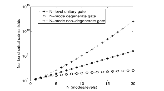
Fig 1: The scaling of the numbers of critical submanifolds for fully non-degenerate ($N$-qunit) symplectic gates and ($N$-qubit) unitary gates.

For a compact target symplectic gate, the critical submanifolds are completely identical when the search is carried out on the full symplectic group (corresponding to linear optics plus squeezing) or its compact subgroup (corresponding to only linear optics), the only difference being an increase in the dimension of the search space. Therefore, the additional directions accessible through squeezing transformations are not expected to improve convergence toward the optimal solution. These observations collectively paint a fairly simple picture of CV gate landscape topology, which, although more complicated than the topology of discrete gate landscapes, should not preclude efficient control optimization.

Throughout this paper, we will use gradient algorithms to optimize the control field. The search process in the kinematic picture can be represented by the so-called gradient flow on the symplectic group:

$$\frac{{\rm d}S}{{\rm d}s}=-\nabla\mathcal{J}(S).$$

It is instructive to estimate the convergence speed of the gradient flow, via linearization of this equation in a sufficiently small neighborhood of the global optimum $S=W$, which gives

$$\frac{{\rm d}~{}\delta S}{{\rm d}s}=-{\rm Hess}(W)~{}\delta S,$$

where $\delta S$ is the deviation of $S$ from $W$, which is proportional to the gradient vector at $S$. The positive definite matrix ${\rm Hess}(W)$ is the Hessian matrix at $W$. Therefore, the convergence of $\delta S$ is exponential and its rate is dominated by the smallest eigenvalue of ${\rm Hess}(W)$, identified as $e_{s}^{-2}\leq 1$. By comparison, a similar estimate for gate search on the discrete unitary group reveals a constant convergence rate of $1$. Therefore, search for noncompact symplectic gates will display slower convergence in general, depending on the magnitudes of the singular values of the target gate. In particular, the convergence speed for the phase gate (or squeezing gate) decreases with increasing phase shift (or squeezing ratio). Fig.2 shows the convergence speed of gradient flows for the SUM gate on the symplectic group, and, for comparison, the CNOT gate on the unitary group.

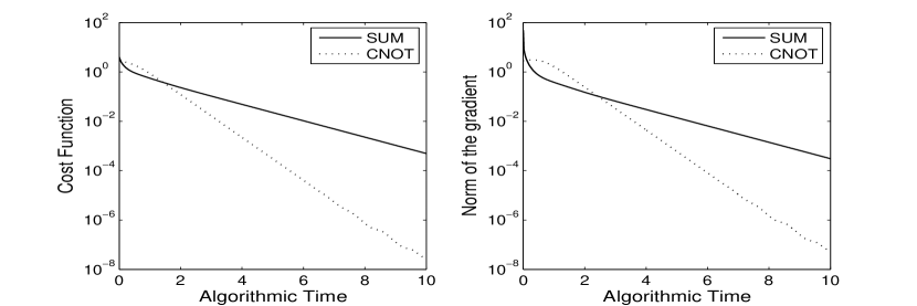
Fig 2: The convergence of the gradient flows for optimal search of the SUM gate on ${\rm Sp}(4,{\mathbb{R}})$ and CNOT gate on $\mathcal{U}(4)$.

V Numerical Simulations

In this section, we numerically solve for optimal control fields for Clifford group gates and composite CV algorithms, and compare the optimization effort and control field complexity to those of the corresponding gates over discrete variables. As such, we aim to identify distinguishing features of CV gate control that will have the greatest impact on its computational and experimental implementation.

V.1 SUM Gate

Consider the control problem where $W$ is the SUM operation, whose matrix form is shown in (7). We simulate the realization of the SUM gate using both the photon model ($\kappa=1$) and the strongly controllable system described above. Fig.3 compares the effects of strong versus weak controllability on convergence speed,starting from either a random guess or near saddle solutions. Although the SUM gate is reachable with both models at the final time, the weaker controllability of the photon model compromises convergence speed. In addition, Fig.4 shows that the corresponding optimal control fields are more expensive in that their fluences are much greater.

The singular values of ${\rm SUM}$ are $E=diag\{1.618,1.618,0.618,0.618\}$. The analysis above predicts that there should be 4 critical submanifolds for a degenerate 2-qunit gate. The first one $D_{1}=diag\{1.618,1.618,0.618,0.618\}$ contains one type-I block, whose corresponding critical submanifold is the isolated global minimum $S^{*}_{1}={\rm SUM}$. The second, $D_{2}=diag\{-0.852,-0.852,-1.174,-1.174\}$, contains one type-II block, whose corresponding critical submanifold is an isolated saddle point. The third, $D_{3}=diag\{1.618,-0.852,-1.174,0.618\}$ contains one type-I and one type-II block. The last saddle contains a type-III block, which actually contains two isolated points. In summary, there are a total of 5 critical submanifolds, including 4 isolated points and 1 one-dimensional manifold. The Hessian analysis is summarized in Table I.

No.	Critical value	$D_{0}$	$D_{+}$	$D_{-}$	type
1	0	0	14	0	minimum
2	18.623	0	10	4	saddle
3	9.311	1	12	1	saddle
4($\pm$)	10	0	11	3	saddle

Table 1: Critical topology for the SUM gate.

As discussed above, the saddles will rarely be encountered during the progress of most optimization trajectories. This is also supported from the simulation result (Fig.3), the saddle manifolds appear to have a slightly adverse effect on optimization efficiency for the strongly controllable system, and almost have no influence on the convergence of the photon model.

Note that the free Hamiltonian for the photon model happens to be proportional to the matrix logarithm of the SUM gate; thus, using this model, SUM can be achieved merely via free evolution in $\kappa^{-1}$ units of time. Simulations show that the SUM gate is always realizable in any time longer than $\kappa^{-1}$ (e.g. Fig.4). However, it is interesting to see if the local controls permit the gate to be achieved in a shorter time. Fig.5 shows an example employing a final time less than $\kappa^{-1}$. As can be seen, the control search does not converge. By contrast, for the strongly controllable system, optimal control fields exist even for very small $t_{f}$, although the expense increases and the shape of control fields tends to become more singular (Fig.6).

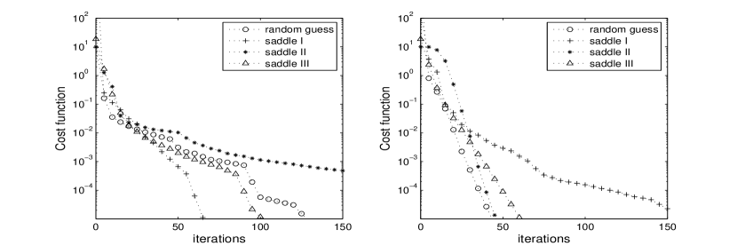
Fig 3: The convergence of dynamical search for the SUM gate using conjugate gradient algorithms with the photon model (left) and a strongly controllable system(right).

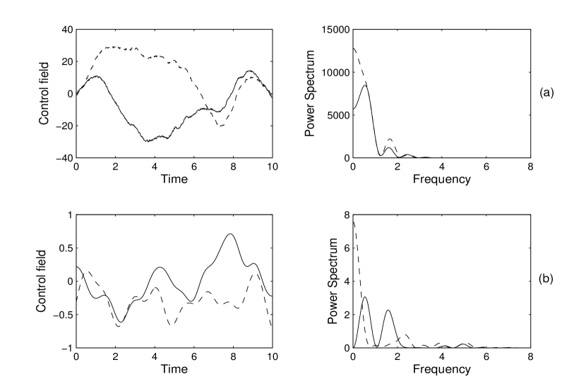
Fig 4: The optimal control fields for CV SUM gate control after searching from a random initial guess, for (a) the photon model and (b) a strongly controllable model.

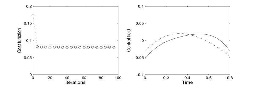
Fig 5: Optimal control search for the SUM gate using conjugate gradient algorithms with the photon model at a final time smaller than $\kappa^{-1}$.

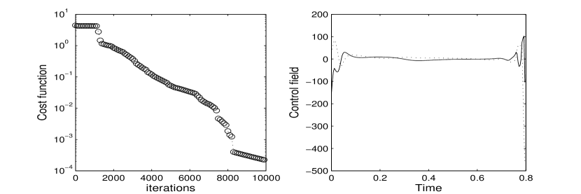
Fig 6: Dynamical search for the SUM gate using conjugate gradient algorithms with the strongly controllable system model at a small final time.

An important feature not shown in the figures is that the optimal search suffers from serious numerical instabilities when it starts far away from $W$ because the system dynamics involves exponentially increasing components. This can easily occur when there is no a priori knowledge of an appropriate choice for the control fields. By contrast, because of the compactness of the dynamical group, the control optimization for discrete quantum systems never encounters this problem.

V.2 SWAP gate

Optimal control landscapes over ${\rm OSp}(2N,{\mathbb{R}})$ and $\mathcal{U}(N)$ have identical topology and geometry, because these dynamical groups are isomorphic. This section simulates the optimal search of a (compact) transform that swaps the states of the two qunits as follows

$$W=\left(\begin{array}[]{cccc}0&1&0&0\\ 1&0&0&0\\ 0&0&0&1\\ 0&0&1&0\\ \end{array}\right).$$

For this gate, we employ the photon model with two local phase controls, using two different free Hamiltonians: (i) $H_{0}=x_{1}p_{2}$, which involves squeezing operations; (ii) $H_{0}=x_{1}p_{2}-x_{2}p_{1}$, which involves only linear optics. It can be verified that these systems are controllable over (i) ${\rm Sp}(4,{\mathbb{R}})$ and (ii) ${\rm OSp}(4,{\mathbb{R}})$, respectively. The simulation results in Fig.7 show that the optimal search restricted on ${\rm OSp}(2N,{\mathbb{R}})$ generally exhibits fast convergence, as in the case of control of discrete unitary gates. This is not surprising because the group ${\rm OSp}(2N,{\mathbb{R}})$ is isomorphic to the unitary group $\mathcal{U}(N)$ and the corresponding dynamical control system is equivalent to a $N$-level discrete quantum control system. By contrast, optimal control using squeezing operators as well exhibits no advantages compared to using only linear operations; in fact, the resulting control fields have much greater fluences (Fig.8).

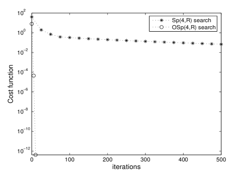
Fig 7: The convergence of optimal search for the SWAP gate with linear and squeezing couplings (${\rm Sp}(4,{\mathbb{R}})$) and linear couplings (${\rm OSp}(4,{\mathbb{R}})$).

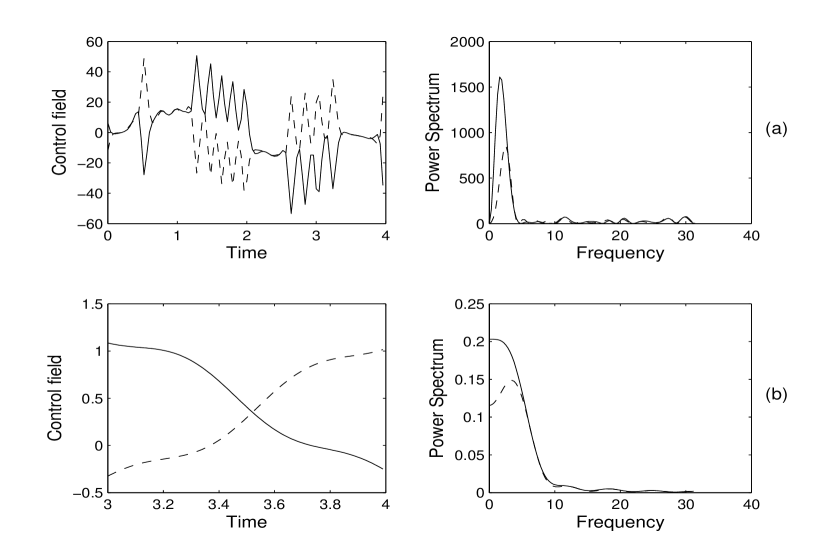
Fig 8: The control fields for the swap gate with (a) linear and squeezing couplings (${\rm Sp}(4,{\mathbb{R}})$) and (b) linear couplings (${\rm OSp}(4,{\mathbb{R}})$) . The solid lines refer to the control field on the first qunit, while the dotted refer to the second.

Because ${\rm OSp}(2N,{\mathbb{R}})$ is isomorphic to $\mathcal{U}(N)$, a comparison of the gradients of the fidelity on ${\rm Sp}(2N,{\mathbb{R}})$ and ${\rm OSp}(2N,{\mathbb{R}})$ sheds light not only on the comparative efficiencies of these two optimization problems, but also the origin of the slower convergence of noncompact CV gate optimization versus that of discrete gate optimization. Fig.9 displays the norm of the gradient of the fidelity of the SWAP gate with respect to the control field on ${\rm Sp}(2N,{\mathbb{R}})$ and ${\rm OSp}(2N,{\mathbb{R}})$, at each algorithmic step during the course of optimization. In order to sample more points along the optimization trajectory, a steepest descent algorithm was employed in this case, starting from near a saddle point of the control landscape. As can be seen, the norm of the gradient is larger on ${\rm OSp}(2N,{\mathbb{R}})$ at most points along the optimization trajectory. In addition, over several runs, it was found that the gradient norm changes more abruptly during optimization on ${\rm Sp}(2N,{\mathbb{R}})$ compared to ${\rm OSp}(2N,{\mathbb{R}})$ (or, equivalently, $\mathcal{U}(N)$). It was also observed that the components of the gradient at successive dynamical time points change abruptly on ${\rm Sp}(2N,{\mathbb{R}})$. These features, presumably originating in the noncompactness of ${\rm Sp}(2N,{\mathbb{R}})$, undoubtedly act to retard the convergence of searches carried out on this group.

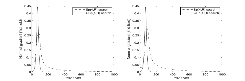
Fig 9: The norm of the gradient vector during optimal search for the SWAP gate, starting from near a saddle point, with linear and squeezing couplings (${\rm Sp}(4,R)$) and linear couplings (${\rm OSp}(4,R)$). The left panel is for the first control field and the right panel is for the second.

V.3 Composite algorithms

Composite algorithms composed of large numbers of low-dimensional Clifford group gates will generally have richer structures in their singular values and a greater number of critical manifolds. The geometry of the control landscape is also expected to be complexified for such gates. In practice, representing composite Clifford group algorithms through sequences of 1-qunit or 2-qunit gates is generally preferred. However, since using a larger number of gates may increase the likelihood of information loss through quantum decoherence, the implementation of higher dimensional transformations is desirable in some instances.

Consider a composite operation on 3 qunits that sums the values of their $q$-components. This gate can be decomposed into two elementary gates ${\rm SUM}(1,2,3)={\rm SUM}(2,3)\times{\rm SUM}(1,2)$, which is represented by

$${\rm SUM}(1,2,3)=\left(\begin{array}[]{cccccc}1&0&0&0&0&0\\ 0&1&0&0&0&0\\ 0&1&1&0&0&0\\ 0&0&0&1&0&0\\ 0&0&0&0&1&-1\\ 0&0&0&0&0&1\\ \end{array}\right)\left(\begin{array}[]{cccccc}1&0&0&0&0&0\\ 1&1&0&0&0&0\\ 0&0&1&0&0&0\\ 0&0&0&1&-1&0\\ 0&0&0&0&1&0\\ 0&0&0&0&0&1\\ \end{array}\right)=\left(\begin{array}[]{cccccc}1&0&0&0&0&0\\ 1&1&0&0&0&0\\ 1&1&1&0&0&0\\ 0&0&0&1&-1&0\\ 0&0&0&0&1&-1\\ 0&0&0&0&0&1\\ \end{array}\right).$$

This composite operation can be implemented using a photon model where the internal Hamiltonian includes interactions between 1-2 and 2-3 qunits, i.e., $H_{0}=x_{1}p_{2}+x_{2}p_{3}$, and three local control Hamiltonians applied in the form of $H_{j}=x_{j}^{2}+p_{j}^{2}$, $j=1,2,3$. Again, because the internal Hamiltonian $H_{0}$ is noncompact, full controllability is not guaranteed at arbitrary final time $t_{f}$. In the case of the ion trap model, the internal Hamiltonian $H_{0}$ consists of uncoupled harmonic oscillators, and two nonlocal controls

$$H_{1}=a^{\dagger}b_{1}+ab_{1}^{\dagger},\quad H_{2}=a^{\dagger}b_{2}^{\dagger}+ab_{2}$$

are applied. As discussed above, there is no guarantee that the gate will be reachable at any final time within this model, since the system does not satisfy the controllability rank condition. In Fig.10, we compare the convergence speeds of optimal control search for the 3-qunit SUM gate using these models with that of its discrete quantum counterpart, the Controlled-CNOT gate (Toffoli gate). In the latter case, the NMR control system described above was used.

As can be seen from Fig.10, neither the ion trap nor the photon control search converges within the specified tolerance for the chosen final time, whereas the strongly controllable system does converge. The weakly controllable and uncontrollable systems therefore display similar behavior for this composite gate. This example demonstrates that the controllability of a CV gate control system may become a more important consideration for higher dimensional gates.

For both discrete and continuous quantum systems, the decrease in convergence speed with increasing system dimension appears to be severe; in addition, control field searches are more likely to become trapped due to easier loss of controllability. Therefore, for a quantum algorithm involving a polynomially large number of operations (i.e., primitive gates), it would indeed appear more efficient to apply sequences of smaller gates rather than attempting global search over transformations on the whole set of qunits. The scaling of optimal control search effort with system size for CV gates is an important subject for future study.

Finally, from Fig.11, we observe a stark difference in the fluence of the optimal control fields obtained using local versus nonlocal controls. For the photon model (local controls), the fluence of the optimal fields exceeds physical limits, whereas for the ion trap model (nonlocal controls) and the NMR model, the fluence remains bounded. This indicates that for composite gates, CV control models employing nonlocal controls may be preferable to those whose design requires the use of local controls. Note that although the NMR model employs local controls, their fluence remains small, suggesting that this problem does not arise for discrete variable gates.

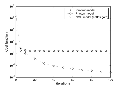
Fig 10: The convergence of optimal searches for the 3-qunit SUM gate with photon model and ion-trap model, and 3-qubit Controlled-CNOT gate with NMR model.

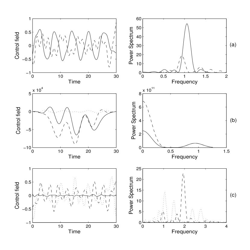
Fig 11: The optimal control fields for (a) 3-qunit SUM gate with ion trap model, (b) 3-qunit SUM gate with photon model and (c) 3-qubit Controlled-CNOT gate. For (b) and (c), the solid (dashed, dotted) lines are the control fields on the first (second, third) qunit/qubit.

VI DISCUSSION

The absence of local traps in control landscapes for symplectic gate fidelity indicates that given sufficient time, local gradient-based algorithms will generally succeed at reaching the global optima (perfect fidelity), assuming the system is controllable. This property, combined with other attractive features of continuous QIP such as the high bandwidth of continuous degrees of freedom, strengthens the feasibility of QIP over continuous variables.

We have seen that CV gate optimization problems can be divided into two classes with inherently different complexities. The first, wherein only linear Hamiltonians are employed as controls, is mathematically identical to the problem of discrete unitary gate optimization. The second, in which squeezing operations are also employed, is generally more expensive.

A second point of distinction between these two control problems is the complexity of the optimal fields. The optimal fields for discrete gate control are typically in resonance with the transition frequencies of the system, within the weak-field regime. By contrast, in the case of CV gate optimization over ${\rm Sp}(2N,{\mathbb{R}})$, the fields are usually not simply related to the natural resonant frequencies of the system because the Hamiltonian possesses imaginary eigenvalues. These eigenvalues produce exponentially increasing and decreasing modes in the field. The former can result in instabilities during the optimization process. Moreover, for CV gate optimization over ${\rm Sp}(2N,{\mathbb{R}})$, there is a strong dependence of field complexity on the final dynamical time. It is important to identify several controllable $t_{f}$’s and choose the one corresponding to control fields that are physically the most simple to implement. However, the higher degeneracy of these fields means that we are presented with more choices for convenient physical implementation, and point to a rich variety of distinct control mechanisms that reach the same objective.

Finally, the effects of quantum system controllability on control optimization are more subtle for CV gate control than for discrete variable gate control. For CV gate control, it is often difficult to identify a final dynamical time $t_{f}$ at which the gate can be reached with high fidelity, if the system is not strongly controllable. Moreover, several current physical models for CV gate synthesis are not fully controllable for any choice of $t_{f}$. For these systems, even when the gate of interest is reachable, the cost of optimal search is typically steep. It is therefore particularly important to employ physical control systems that satisfy the conditions for controllability.

These details must be borne in mind when assessing the comparative difficulty of implementing quantum communication protocols over continuous versus discrete variables, and underscore the importance of using optimal control theory in the design of high-fidelity symplectic gates. An important conclusion of this work is that it is important to use the methodology of control theory when designing physical systems for the implementation of continuous variable quantum gates, both in the choice of appropriate physical systems and in the determination of the controls themselves. Application of OCT to practical CV quantum information tasks will require the imposition of penalty terms on the control Hamiltonians corresponding to physical constraints. For control of discrete states in molecular systems, the most significant constraint on the control fields is the total fluence, since current pulse shaping technologies are capable of producing the majority of shapes predicted by OCT. Ongoing efforts to design pulse shapers with ultra high bandwidth should further facilitate implementation of the theoretically predicted fields. By contrast, for CV systems, it is difficult to shape control pulses within certain physical models. Applying shape constraints to the optimization problems above would amount to choosing amongst the highly degenerate sets of control Hamiltonians that solve the generic OCT problem.

In the context of particular Hamiltonians, time optimal control theory has been applied to assess the minimal time necessary to implement various primitive discrete quantum gates Khaneja and Glaser (2001); Khaneja et al. (2001, 2002). A natural counterpart to the current work is the application of time optimal control theory to symplectic gates, using restricted control Hamiltonians that are commonly implemented in the quantum optics laboratory. Given the susceptibility of CV quantum systems to noise, time optimal control of CV gates is particularly relevant. Such studies would necessitate determination of the minimal length geodesics in the noncompact symplectic group, or in subgroups of ${\rm Sp}(2N,{\mathbb{R}})$ that can be reached using the restricted controls. Preliminary work Braunstein (2005) along these lines employing the so-called Bloch-Messiah theorem has been reported, but it is unlikely that analytical solutions exist for most time optimal symplectic transformation control problems, especially for higher qunit systems. As such, the development of numerical OCT algorithms suited to time-optimal CV gate control is an important future challenge.

In the present work, we have adopted the approach of optimizing a scalar objective function for gate fidelity. An alternative approach would be to track a predefined trajectory on the space of symplectic propagators between the initial and target gate. From a local perspective, the former is computationally more efficient, but globally, the latter may offer an advantage. Perhaps more importantly, the latter approach would provide insight into the effect of the map between control fields and dynamical propagators on optimization efficiency. Indeed, the numerical simulations above indicate that the properties of this map are primarily responsible for the differences in optimization efficiency between discrete and CV quantum OCT. Moreover, these properties will impact the efficiency of control optimization for any observable of a quadratic CV system, since the symplectic transformation uniquely defines the infinite-dimensional unitary propagator corresponding to the CV quantum dynamical process.

Finally, we note that universal quantum computation requires nonlinear symplectic gates corresponding to the ability to count photons in the electromagnetic field Lloyd and Slotine (1998). The implementation of nonlinear symplectic gates necessary to achieve universal continuous quantum computation is known to be difficult to achieve with high fidelity Gottesman et al. (2001). Purification protocols are necessary to distill from an initial supply of noisy nonlinear symplectic states a smaller number of such states with higher fidelity. Future work should consider the challenges inherent in implementing such gates through the methodology of optimal control theory.