A posteriori error estimates for finite element approximations of the Cahn-Hilliard equation and the Hele-Shaw flow

Abstract

This paper develops a posteriori error estimates of residual type for conforming and mixed finite element approximations of the fourth order Cahn-Hilliard equation $u_{t}+{\Delta}\bigl{(}{\varepsilon}{\Delta}u-{\varepsilon}^{-1}f(u)\bigr{)}=0$. It is shown that the a posteriori error bounds depends on ${\varepsilon}^{-1}$ only in some low polynomial order, instead of exponential order. Using these a posteriori error estimates, we construct an adaptive algorithm for computing the solution of the Cahn-Hilliard equation and its sharp interface limit, the Hele-Shaw flow. Numerical experiments are presented to show the robustness and effectiveness of the new error estimators and the proposed adaptive algorithm.

1 Introduction

In this paper we derive a posteriori error estimates and develop an adaptive algorithm based on the error estimates for conforming and mixed finite element approximations of the following Cahn-Hilliard equation and its sharp interface limit known as the Hele-Shaw flow [2, 37]

(1) $$u_{t}+{\Delta}\bigl{(}{\varepsilon}{\Delta}u-\frac{1}{{\varepsilon}}f(u)\bigr{)} = 0\quad\mbox{ in }{\Omega}_{T}:={\Omega}\times(0,T),$$

(2) $$\frac{\partial u}{\partial n}=\frac{\partial}{\partial n}\bigl{(}{\varepsilon}{\Delta}u-\frac{1}{{\varepsilon}}f(u)\bigr{)} = 0\quad\mbox{ in }\partial{\Omega}_{T}:=\partial{\Omega}\times(0,T),$$

(3) $$u = u_{0}\quad\mbox{in }{\Omega}\times\{0\},$$

where ${\Omega}\subset\mathbf{R}^{N}$ $(N=2,3)$ is a bounded domain with $C^{2}$ boundary $\partial{\Omega}$ or a convex polygonal domain. $T>0$ is a fixed constant, and $f$ is the derivative of a smooth double equal well potential taking its global minimum value $0$ at $u=\pm 1$. A well known example of $f$ is

$$f(u):=F^{\prime}(u)\quad\mbox{and}\quad F(u)=\frac{1}{4}(u^{2}-1)^{2}.$$

For the notation brevity, we shall suppress the super-index ${\varepsilon}$ on $u^{\varepsilon}$ throughout this paper except in Section 5.

The equation (1) was originally introduced by Cahn and Hilliard [11] to describe the complicated phase separation and coarsening phenomena in a melted alloy that is quenched to a temperature at which only two different concentration phases can exist stably. The Cahn-Hilliard has been widely accepted as a good (conservative) model to describe the phase separation and coarsening phenomena in a melted alloy. The function $u$ represents the concentration of one of the two metallic components of the alloy. The parameter $\varepsilon$ is an “interaction length”, which is small compared to the characteristic dimensions on the laboratory scale. Cahn-Hilliard equation (1) is a special case of a more complicated phase field model for solidification of a pure material [10, 29, 33]. For the physical background, derivation, and discussion of the Cahn-Hilliard equation and related equations, we refer to [4, 2, 7, 11, 13, 20, 35, 36] and the references therein. It should be noted that the Cahn-Hilliard equation (1) can also be regarded as the $H^{-1}$-gradient flow for the energy functional [28]

(4) $${\mathcal{J}}_{\varepsilon}(u):=\int_{\Omega}\Bigl{[}\,\frac{1}{2}|\nabla u|^{2}+\frac{1}{{\varepsilon}^{2}}F(u)\,\Bigr{]}\,dx.$$

In addition to its application in phase transition, the Cahn-Hilliard equation (1) has also been extensively studied in the past due to its connection to the following free boundary problem, known as the Hele-Shaw problem and the Mullins-Sekerka problem

(5) $${\Delta}w =0 \quad\mbox{in }{\Omega}\setminus{\Gamma}_{t},\,t\in[0,T]\,,$$

(6) $$\frac{{\partial}w}{{\partial}n} =0 \quad\mbox{on }{\partial}{\Omega},\,t\in[0,T]\,,$$

(7) $$w =\sigma\kappa \quad\mbox{on }{\Gamma}_{t},\,t\in[0,T]\,,$$

(8) $$V =\frac{1}{2}\Bigl{[}\frac{{\partial}w}{{\partial}n}\Bigr{]}_{{\Gamma}_{t}} \quad\mbox{on }{\Gamma}_{t},\,t\in[0,T]\,,$$

(9) $${\Gamma}_{0} ={\Gamma}_{00} \quad\mbox{when }t=0\,.$$

Here

$$\sigma=\int_{-1}^{1}\sqrt{\frac{F(s)}{2}}\,{\rm d}s\,.$$

$\kappa$ and $V$ are, respectively, the mean curvature and the normal velocity of the interface ${\Gamma}_{t}$, $n$ is the unit outward normal to either ${\partial}{\Omega}$ or ${\Gamma}_{t}$, $[\frac{{\partial}w}{{\partial}n}]_{{\Gamma}_{t}}:=\frac{{\partial}w^{+}}{{\partial}n}-\frac{{\partial}w^{-}}{{\partial}n}$, and $w^{+}$ and $w^{-}$ are respectively the restriction of $w$ in ${\Omega}^{+}_{t}$ and ${\Omega}^{-}_{t}$, the exterior and interior of ${\Gamma}_{t}$ in ${\Omega}$.

Under certain assumption on the initial datum $u_{0}$, it was first formally proved by Pego [37] that, as $\varepsilon\searrow 0$, the function $w^{\varepsilon}:=-{\varepsilon}{\Delta}u^{\varepsilon}+{\varepsilon}^{-1}f(u^{\varepsilon})$, known as the chemical potential, tends to $w$, which, together with a free boundary ${\Gamma}:=\cup_{0\leq t\leq T}({\Gamma}_{t}\times\{t\})$ solves (5)-(9). Also $u^{\varepsilon}\rightarrow\pm 1$ in ${\Omega}_{t}^{\pm}$ for all $t\in[0,T]$, as ${\varepsilon}\searrow 0$. The rigorous justification of this limit was carried out by Alikakos, Bates and Chen in [2] under the assumption that the above Hele-Shaw (Mullins-Sekerka) problem has a classical solution. Later, Chen [13] formulated a weak solution to the Hele-Shaw (Mullins-Sekerka) problem and showed, using an energy method, that the solution of (1)-(3) approaches, as ${\varepsilon}\searrow 0$, to a weak solution of the Hele-Shaw (Mullins-Sekerka) problem. One of a consequences of the connection between the Cahn-Hilliard equation and the Hele-Shaw flow is that for small $\varepsilon$ the solution to (1)-(3) equals $\pm 1$ in the two bulk regions of ${\Omega}$ which is separated by a thin layer (called diffuse interface) of width $O(\epsilon)$. As expected, the solution has a sharp moving front over the transition layer.

Another motivation for developing efficient adaptive numerical methods for the Cahn-Hilliard equation is its applications far beyond its original role in phase transition. The Cahn-Hilliard equation is indeed a fundamental equation and an essential building block in the phase field theory for moving interface problems (cf. [31]), it is often combined with other fundamental equations of mathematical physics such as the Navier-Stokes equation (cf. [22, 30, 34] and the references therein) to be used as diffuse interface models for describing various interface dynamics, such as flow of two-phase fluids, from various applications.

The primary numerical challenge for solving the Cahn-Hilliard equation results from the presence of the small parameter $\varepsilon$ in the equation, so the equation is a singular perturbation of the biharmonic heat equation. Numerically to resolve the thin transition region of width $O(\varepsilon)$, one has to use very fine meshes in the region. Considering the fact that away from the transition region the solution equals $\pm 1$, it is natural to use adaptive meshes, rather than uniform meshes, to compute the solution. As far as the error analysis concerns, the main difficulty is to derive a priori and a posteriori error estimates which depends on $\frac{1}{\varepsilon}$ only in (low) polynomial order, rather than exponential order which is the case if the standard Gronwall’s inequality type argument is used to derive the error estimates [6, 17, 18, 19]. Recently, Feng and Prohl [25, 26, 24] were able to overcome this difficulty and established polynomial order a priori error estimates for mixed finite element approximations of the Cahn-Hilliard equation and related phase field equations. Based on these new error estimates, they then proved convergence of the numerical solutions of the phase field equations to the solutions of their respective sharp interface limits as mesh sizes and the parameter ${\varepsilon}$ all tend to zero. The main idea of [25, 26] is to use a spectral estimate result of Alikakos and Fusco [3] and Chen [12] for the linearized Cahn-Hilliard operator to handle the nonlinear term in the error equation. Very recently, this idea was also used by Kessler, Nochetto and Schmidt [32] and by Feng and Wu [27] to obtain a posteriori error estimates, which depend on $\frac{1}{{\varepsilon}}$ in some low polynomial order, for finite element approximations of the Allen-Cahn equation.

The goal of this paper is to develop a posteriori error estimates for conforming and mixed finite element approximations of the Cahn-Hilliard equation in the spirit of [27]. First, using the idea of continuous dependence we derive some residual type a posteriori error estimates, which depend on $\frac{1}{{\varepsilon}}$ only in low polynomial orders, for the conforming finite element approximations and the mixed finite element approximations. To avoid many technicalities and to present the idea, we only consider semi-discrete (in spatial variable) approximations in this paper. For the time discretization, we appeal to the stiff ODE solver NDF [40] which is a modification of BDF for temporal integration. Then, using the a posteriori estimates as error indicators we propose an adaptive algorithm for approximating the Cahn-Hilliard equation and its sharp interface limit, the Hele-Shaw flow. As in [27], the technique and analysis of this paper for deriving a posteriori error estimates are problem-independent and method-independent, hence, they are applicable to a large class of evolution problems and their numerical approximations obtained by any (numerical) discretization method including finite difference, finite element, finite volume and spectral methods. We also remark that the adaptive finite element algorithm of this paper is based on the method of lines approach, we refer to [1, 5, 21] and the references therein for a detailed exposition on the approach for other types of problems, and to [21, 41] and the references therein for a detailed discussions about adaptive algorithms based on other approaches such as discontinuous Galerkin methods and space-time finite element methods.

The paper is organized as follows: In Section 2 we establish continuous dependence estimates for the Cahn-Hilliard equation in both standard and mixed formulations, and present some abstract frameworks for deriving a posteriori error estimates based on the idea of continuous dependence. In Section 3 we derive some a posteriori error estimates for conforming finite element approximations and for the Ciarlet-Raviart mixed finite element approximations of the Cahn-Hilliard equation using the continuous dependence estimates and the abstract frameworks of Section 2. In Section 4 we propose an adaptive finite element algorithm using the a posteriori error estimates of Section 3 as error indicators for refining or coarsening the mesh. In Section 5 we establish some a posteriori error estimates for using the conforming and mixed finite element methods to approximate the Hele-Shaw flow. Finally, in Section 6 we present several numerical tests to show the robustness and effectiveness of the proposed error estimators and the adaptive algorithm.

2 Continuous dependence and a posteriori error estimates

In this section, we first establish some continuous dependence (on nonhomogeneous force term and on initial condition) estimates for the Cahn-Hilliard problem (1)-(3) in both standard and mixed formulations. We then present an abstract framework for deriving a posteriori error estimates for mixed numerical approximations of general evolution equations. Our goal is to derive a posteriori error estimates which depend on $\frac{1}{{\varepsilon}}$ only in some low polynomial order. It is easy to show that (cf. Section 2.1 ) if one uses the standard perturbation and Gronwall’s inequality techniques to derive a priori or a posteriori error estimates, the error bounds will depend on $\frac{1}{{\varepsilon}}$ exponentially, hence, such estimates are not useful for small $\varepsilon$. To overcome the difficulty, we appeal to a spectrum estimate result, due to Alikakos and Fusco [3] and Chen [12], for the linearized Cahn-Hilliard operator, and prove a continuous dependence estimate, which depends on $\frac{1}{{\varepsilon}}$ in some low polynomial order, for the Cahn-Hilliard equation. Such a continuous dependence estimate is the key for us to establish the desired a posteriori error estimates in the next section.

Throughout this paper, the standard space, norm and inner product notation are adopted. Their definitions can be found in [8, 15]. In particular, $(\cdot,\cdot)$ denotes the standard $L^{2}$-inner product, and $H^{k}({\Omega})$ stands for the usual Sobolev spaces. Also, $C$ are used to denote a generic positive constant which is independent of $\varepsilon$ and the mesh sizes.

2.1 Continuous dependence estimates

Introduce the space

$$H^{2}_{E}({\Omega})=\left\{\psi\in H^{2}({\Omega});\;\frac{\partial\psi}{\partial n}=0\text{ on }\partial{\Omega}\right\}.$$

We recall that the variational formulation of (1)–(3) is defined by seeking $u\in H^{2}_{E}({\Omega})$ such that

(10) $$\langle u_{t},\psi\rangle+{\varepsilon}\bigl{(}{\Delta}u,{\Delta}\psi\bigr{)}+\frac{1}{{\varepsilon}}\bigl{(}{\nabla}(f(u)),{\nabla}\psi\bigr{)} =0\quad\forall\psi\in H^{2}({\Omega}),\;t\in[0,T],$$

(11) $$u(0) =u_{0}\in H^{2}_{E}({\Omega}).$$

It is proved in [18] that such a solution $u$ exists and

$$u\in L^{\infty}((0,T);H^{2}_{E}({\Omega}))\cap L^{2}((0,T);H^{4}({\Omega}))\cap H^{1}((0,T);L^{2}({\Omega})).$$

For physical reason, unless mentioned otherwise, we assume that $|u_{0}|\leq 1$ in this paper.

Let $v(t)\in H^{2}_{E}({\Omega})$ be a perturbation of $u$ satisfying

(12) $$\left\langle v_{t},\psi\right\rangle+{\varepsilon}\bigl{(}{\Delta}v,{\Delta}\psi\bigr{)}+\frac{1}{{\varepsilon}}\bigl{(}{\nabla}(f(v)),{\nabla}\psi\bigr{)}=\left\langle r(t),\psi\right\rangle \quad\forall\psi\in H^{2}_{E}({\Omega}),\;t\in[0,T],$$

(13) $$v(0)=v_{0}\in H^{2}_{E}({\Omega}),$$

where $r(t)\in{\widetilde{H}^{-2}(\Omega)}:=(H^{2}_{E}({\Omega}))^{*}$ (the dual space of $H^{2}_{E}({\Omega})$) is the residual of $v(t)$, i.e., the perturbation of the right-hand side of (1). $\left\langle\cdot,\cdot\right\rangle$ denotes the dual product on ${\widetilde{H}^{-2}(\Omega)}\times H^{2}({\Omega})$. We assume that $\left\langle r(t),1\right\rangle=0$, and define

(14) $$\left\|r(t)\right\|_{{\widetilde{H}^{-2}}}=\sup_{0\neq\psi\in H^{2}_{E}({\Omega})}\frac{\left\langle r(t),\psi\right\rangle}{\left\|\psi\right\|_{H^{2}}}.$$

Let $L^{2}_{0}({\Omega})=\left\{\psi\in L^{2}({\Omega});\;\int_{\Omega}\psi dx=0\right\}$. Define ${\Delta}^{-1}:L^{2}_{0}({\Omega})\rightarrow H^{1}({\Omega})\cap L^{2}_{0}({\Omega})$ to be the inverse of the Laplacian ${\Delta}$, that is, for any $\psi\in L^{2}_{0}({\Omega})$, ${\Delta}^{-1}\psi\in H^{1}({\Omega})\cap L^{2}_{0}({\Omega})$ is defined by

$$\bigl{(}{\nabla}({\Delta}^{-1}\psi),{\nabla}\eta\bigr{)}=-(\psi,\eta)\qquad\forall\eta\in H^{1}({\Omega}).$$

From the standard regularity theory of elliptic problems, one concludes that ${\Delta}^{-1}\psi\in H^{2}_{E}({\Omega})$ and

(15) $$\left\|{\Delta}^{-1}\psi\right\|_{H^{2}({\Omega})}\leq C\left\|\psi\right\|_{L^{2}}.$$

Let $w(t):=v(t)-u(t)$. We also assume that $w(0)=v_{0}-u_{0}\in L^{2}_{0}({\Omega})$. Then, from $\int_{\Omega}w(t)dx=\int_{\Omega}w(0)dx$, it is clear that $w(t)\in L^{2}_{0}({\Omega})$. Subtracting equation (10) from equation (12) gives

(16) $$\left\langle w_{t},\psi\right\rangle+{\varepsilon}\bigl{(}{\Delta}w,{\Delta}\psi\bigr{)}+\frac{1}{{\varepsilon}}\bigl{(}{\nabla}(f(v)-f(u)),{\nabla}\psi\bigr{)}=\left\langle r(t),\psi\right\rangle\quad\forall\psi\in H^{2}_{E}({\Omega}).$$

Next, we give two estimates on $u-v$ in terms of $r$ and $u_{0}-v_{0}$ for the Cahn-Hilliard equation. The first estimate holds without any constraint on either the initial condition or the residual of the perturbation problem, but the estimate depends on $\frac{1}{\varepsilon}$ exponentially. The second one, which depends on $\frac{1}{\varepsilon}$ only in a low polynomial order, holds provided that the perturbations of the initial condition and the right-hand side are small.

Proposition 1.

Let $u$ and $v$ be the weak solutions of (10)-(11) and (12)-(13), respectively. Then it holds that for $t\in[0,T]$

(17) $$\begin{split}&\left\|{\nabla}{\Delta}^{-1}(v(t)-u(t))\right\|_{L^{2}}^{2}+{\varepsilon}\int_{0}^{t}\exp\Bigl{(}\frac{4(t-s)}{{\varepsilon}^{3}}\Bigr{)}\left\|{\nabla}(v(s)-u(s))\right\|_{L^{2}}^{2}\,ds\\ &\hskip 21.68121pt\leq\exp\Bigl{(}\frac{4t}{{\varepsilon}^{3}}\Bigr{)}\,\left\|{\nabla}{\Delta}^{-1}(v_{0}-u_{0})\right\|_{L^{2}}^{2}+\frac{C}{{\varepsilon}}\int_{0}^{t}\exp\Bigl{(}\frac{4(t-s)}{{\varepsilon}^{3}}\Bigr{)}\left\|r(s)\right\|_{{\widetilde{H}^{-2}}}^{2}\,ds.\end{split}$$

Proof.

Setting $\psi=-{\Delta}^{-1}w$ in (16) we get

(18) $$\frac{1}{2}\frac{d}{dt}\left\|{\nabla}{\Delta}^{-1}w\right\|_{L^{2}}^{2}+{\varepsilon}\left\|{\nabla}w\right\|_{L^{2}}^{2}+\frac{1}{{\varepsilon}}\bigl{(}f(v)-f(u),w\bigr{)}=-\left\langle r,{\Delta}^{-1}w\right\rangle.$$

From the definition of ${\Delta}^{-1}$ it follows

(19) $$\left\|w\right\|_{L^{2}}^{2}=\bigl{(}{\nabla}({\Delta}^{-1}w),{\nabla}w\bigr{)}\leq\left\|{\nabla}({\Delta}^{-1}w)\right\|_{L^{2}}\left\|{\nabla}w\right\|_{L^{2}}.$$

Hence,

$$\frac{1}{{\varepsilon}}\bigl{(}f(v)-f(u),w\bigr{)} =\frac{1}{{\varepsilon}}\bigl{(}f^{\prime}(\xi)w,w\bigr{)}=\frac{1}{{\varepsilon}}\bigl{(}(3\xi^{2}-1)w,w\bigr{)}\geq-\frac{1}{{\varepsilon}}\left\|w\right\|_{L^{2}}^{2}$$

$$\geq-\frac{{\varepsilon}}{4}\left\|{\nabla}w\right\|_{L^{2}}^{2}-\frac{1}{{\varepsilon}^{3}}\left\|{\nabla}({\Delta}^{-1}w)\right\|_{L^{2}}^{2}.$$

Similarly,

$$-\left\langle r,{\Delta}^{-1}w\right\rangle \leq\left\|r\right\|_{{\widetilde{H}^{-2}}}\left\|{\Delta}^{-1}w\right\|_{H^{2}}\leq C\left\|r\right\|_{{\widetilde{H}^{-2}}}\left\|w\right\|_{L^{2}}\leq C{\varepsilon}\left\|r\right\|_{{\widetilde{H}^{-2}}}^{2}+\frac{1}{{\varepsilon}}\left\|w\right\|_{L^{2}}^{2}$$

$$\leq C{\varepsilon}\left\|r\right\|_{{\widetilde{H}^{-2}}}^{2}+\frac{{\varepsilon}}{4}\left\|{\nabla}w\right\|_{L^{2}}^{2}+\frac{1}{{\varepsilon}^{3}}\left\|{\nabla}({\Delta}^{-1}w)\right\|_{L^{2}}^{2}.$$

Combining the above two estimates and (18) we obtain

$$\frac{d}{dt}\left\|{\nabla}{\Delta}^{-1}w\right\|_{L^{2}}^{2}+{\varepsilon}\left\|{\nabla}w\right\|_{L^{2}}^{2}\leq\frac{4}{{\varepsilon}^{3}}\left\|{\nabla}({\Delta}^{-1}w)\right\|_{L^{2}}^{2}+C{\varepsilon}\left\|r\right\|_{{\widetilde{H}^{-2}}}^{2}.$$

Finally, the desired estimate (17) follows from an application of the Gronwall’s inequality. The proof is complete. ∎

Remark 2.1.

Clearly, the above continuous dependence estimates are only useful when $t=O({\varepsilon}^{3})$. However, the estimate is sharp if no assumptions on the solutions $u$ and $v$ are assumed because the Cahn-Hilliard equation does exhibit a fast initial transient regime for times of order $O(\varepsilon^{3})$, until interfaces develop [11, 2].

To improve estimates (17), we need to confine ourself to consider solutions $u$ and $v$ which have certain profiles. Specifically, we need the helps of the following three lemmas. The first lemma gives an a priori estimate for solutions of a Bernoulli type nonlinear ordinary differential inequality. Its proof can be found in [27].

Lemma 2.

Suppose that $n>1$, $y(t)$ and $\lambda(t)$ are nonnegative functions satisfying

(20) $$y^{\prime}(t)\leq\lambda(t)\,(y(t))^{n}+a(t)y(t)+b(t)\qquad\forall t\in[0,T]\,.$$

Define $\rho(t)=\int_{0}^{t}e^{-\int_{0}^{s}a(\tau)\,d\tau}b(s)\,ds$ and $\bar{\rho}(t)=\max_{0\leq s\leq t}\rho(s)$, then there holds for $t\in[0,T^{*})$

(21) $$y(t)\leq\frac{[y(0)+\bar{\rho}(t)]\,e^{\int_{0}^{t}a(s)\,ds}}{\zeta(t)^{\frac{1}{n-1}}}+[\rho(t)-\bar{\rho}(t)]e^{\int_{0}^{t}a(s)\,ds},$$

where

$$\zeta(t)=1-(n-1)\,[y(0)+\bar{\rho}(t)]^{n-1}\int_{0}^{t}\,\lambda(s)\,e^{(n-1)\int_{0}^{s}a(\tau)\,d\tau}\,ds,$$

and $T^{*}$ is the largest positive number in $[0,T]$ such that $\zeta(t)\geq 0$ .

The second lemma cites a spectrum estimate result of Alikakos and Fusco [3] and Chen [12] for the following linearized Cahn-Hilliard operator at the solution of (1)-(3)

(22) $${\mathcal{L}}_{CH}:={\Delta}\bigl{(}{\varepsilon}{\Delta}-\frac{1}{{\varepsilon}}f^{\prime}(u)I\bigr{)},$$

where $I$ stands for the identity operator.

Lemma 3.

Let $\lambda_{CH}$ denote the smallest eigenvalue of ${\mathcal{L}}_{CH}$, assume that the solution $u$ satisfies the $\tanh$ profile described in [12] (cf. (1.10) on page 1374 and Theorem 1.1 on page 1375 of [12]). Then there exists $0<\varepsilon_{0}<1$ and an $\varepsilon$-independent positive constant $C_{0}$ such that $\lambda_{CH}$ satisfies

$$\lambda_{CH}\equiv\inf_{0\not\equiv\psi\in H^{1}({\Omega})\cap L^{2}_{0}({\Omega})}\frac{\varepsilon\,\left\|\nabla\psi\right\|_{L^{2}}^{2}+\frac{1}{\varepsilon}\,(f^{\prime}(u)\psi,\psi)}{\left\|{\nabla}{\Delta}^{-1}\psi\right\|_{L^{2}}^{2}}\geq-C_{0}\qquad\forall\varepsilon\in(0,\varepsilon_{0}].$$

Remark 2.2.

Since the proof of the above estimate is based on the convergence result of [14], which says that the solution of the Cahn-Hilliard problem (1)-(3) for certain class of initial conditions converges to the classical solution of the free boundary problem (5)-(9) as $\varepsilon\rightarrow 0$, hence, the proof suggests that the validity of the above estimate also depends on the choice of the initial conditions. As far as we know it is an open question whether the estimate still holds for “general” initial data (see Remark 2.3 of [14] for more discussions). This is the reason why the subsequent a posteriori error estimates of this paper are established under this initial condition constraint.

The third lemma gives an estimate which are useful for the subsequent analysis.

Lemma 4.

Let $0<{\delta}<2$, then there exits a positive constant $C$ which is independent of $\varepsilon$ and ${\delta}$ such that for any $w\in H^{1}({\Omega})\cap L^{2}_{0}({\Omega})$ there holds

(23) $$\frac{1}{{\varepsilon}}\int_{\Omega}\left|w\right|^{3}\,dx\leq\frac{1}{2{\varepsilon}}\left\|w\right\|_{L^{4}}^{4}+\frac{{\varepsilon}^{4}}{4}\left\|{\nabla}w\right\|_{L^{2}}^{2}+C{\delta}{\varepsilon}^{4-\frac{20}{{\delta}}}\left\|{\nabla}{\Delta}^{-1}w\right\|_{L^{2}}^{\frac{16+2(N-2){\delta}}{(2+N){\delta}}}.$$

Proof.

Recall the Young’s inequality

$$ab\leq\frac{q-1}{q}a^{\frac{q}{q-1}}+\frac{b^{q}}{q},\qquad a,b>0,q>1.$$

Hence,

(24) $$ab\leq a^{\frac{q}{q-1}}+\big{(}1-\frac{1}{q}\big{)}^{q}\frac{b^{q}}{q-1}\leq a^{\frac{q}{q-1}}+e^{-1}\frac{b^{q}}{q-1}.$$

Then for $2<p<3$

$$\left|w\right|^{3}=\left(\frac{\left|w\right|^{4}}{2}\right)^{\frac{3-p}{4-p}}2^{\frac{3-p}{4-p}}\left|w\right|^{\frac{p}{4-p}}\leq\frac{\left|w\right|^{4}}{2}+C\left|w\right|^{p},$$

therefore,

(25) $$\frac{1}{{\varepsilon}}\int_{\Omega}|w|^{3}\,dx\leq\frac{1}{2{\varepsilon}}\left\|w\right\|_{L^{4}}^{4}+\frac{C}{{\varepsilon}}\left\|w\right\|_{L^{p}}^{p}.$$

Since $w\in H^{1}({\Omega})\cap L^{2}_{0}({\Omega})$, it follows from the Sobolev inequality and (19) that

$$\left\|w\right\|_{L^{p}}\leq\left\|w\right\|_{L^{2}}^{1-\frac{N(p-2)}{2p}}\left\|{\nabla}w\right\|_{L^{2}}^{\frac{N(p-2)}{2p}}\leq C\left\|{\nabla}{\Delta}^{-1}w\right\|_{L^{2}}^{\frac{2p-N(p-2)}{4p}}\left\|{\nabla}w\right\|_{L^{2}}^{\frac{2p+N(p-2)}{4p}}.$$

Let $p=\frac{8+2N-2{\delta}}{2+N}=2+\frac{2(2-{\delta})}{2+N}$, we have

$$\frac{1}{{\varepsilon}}\left\|w\right\|_{L^{p}}^{p} \leq C{\varepsilon}^{-5+{\delta}}\left(\frac{{\varepsilon}^{4}}{4}\left\|{\nabla}w\right\|_{L^{2}}^{2}\right)^{\frac{4-{\delta}}{4}}\left\|{\nabla}{\Delta}^{-1}w\right\|_{L^{2}}^{\frac{8+(N-2){\delta}}{2(2+N)}}.$$

From inequality (24) with $q=\frac{4}{{\delta}}$ we obtain

$$\frac{1}{{\varepsilon}}\left\|w\right\|_{L^{p}}^{p} \leq\frac{{\varepsilon}^{4}}{4}\left\|{\nabla}w\right\|_{L^{2}}^{2}+C{\delta}{\varepsilon}^{4-\frac{20}{{\delta}}}\left\|{\nabla}{\Delta}^{-1}w\right\|_{L^{2}}^{\frac{16+2(N-2){\delta}}{(2+N){\delta}}}.$$

(23) now follows from combining the above estimate and (25). The proof is complete. ∎

We are now ready to state our first main result of this section.

Proposition 5.

Suppose that $|u_{0}|,|v_{0}|\leq 1$, ${\varepsilon}_{0}$ and $C_{0}$ be the same as in Lemma 3. Let $u$ and $v$ be the solutions of (10)-(11) and (12)-(13), respectively. Then, for any $\varepsilon\in(0,\varepsilon_{0}]$, there exists a positive constant $C$, which is independent of ${\varepsilon}$ and $t$, such that there holds

(26) $$\begin{split}&\left\|{\nabla}{\Delta}^{-1}(v(t)-u(t))\right\|_{L^{2}}^{2}\\ &\qquad+\int_{0}^{t}\,\Bigl{(}{\varepsilon}^{4}\left\|\nabla(v(s)-u(s))\right\|_{L^{2}}^{2}+\frac{1}{{\varepsilon}}\left\|v(s)-u(s)\right\|_{L^{4}}^{4}\Bigr{)}e^{(2C_{0}+8)(t-s)}\,ds\\ &\leq\frac{1}{\xi(t)}\left\|{\nabla}{\Delta}^{-1}(v_{0}-u_{0})\right\|_{L^{2}}^{2}e^{(2C_{0}+8)t}\\ &\qquad+\Bigl{[}1+\frac{1}{\xi(t)}\Bigr{]}C{\varepsilon}^{-2}\int_{0}^{t}\,\left\|r(s)\right\|_{{\widetilde{H}^{-2}}}^{2}e^{(2C_{0}+8)(t-s)}\,ds\end{split}$$

for all $t\in[0,T^{*})$. Here

(27) $$\begin{split}\xi(t):=&1-C{\varepsilon}^{-\frac{5(2+N)}{2}}e^{(2C_{0}+8)t}\times\\ &\qquad\left\{\left\|{\nabla}{\Delta}^{-1}(v_{0}-u_{0})\right\|_{L^{2}}^{2}+{\varepsilon}^{-2}\int_{0}^{t}\,\left\|r(s)\right\|_{{\widetilde{H}^{-2}}}^{2}\,e^{-(2C_{0}+8)s}\,ds\right\},\end{split}$$

and $T^{*}\in[0,T]$ satisfying $\xi(T^{*})>0$.

Proof.

Let $w:=v-u$, from (18) and the identities

(28) $$f(v)-f(u) =f^{\prime}(u)w+w^{3}+3uw^{2},$$

$$\bigl{(}f(v)-f(u),w\bigr{)} =\int_{\Omega}f^{\prime}(u)\,w^{2}\,dx+\left\|w\right\|_{L^{4}}^{4}+3\int_{\Omega}u\,w^{3}\,dx,$$

and the fact that $\left\|u\right\|_{L^{\infty}}\leq C$ (cf. [9, 26]) we have

(29) $$\begin{split}&\frac{1}{2}\frac{d}{dt}\left\|{\nabla}{\Delta}^{-1}w\right\|_{L^{2}}^{2}+\frac{1}{{\varepsilon}}\left\|w\right\|_{L^{4}}^{4}+{\varepsilon}\left\|\nabla w\right\|_{L^{2}}^{2}+\frac{1}{{\varepsilon}}\int_{\Omega}f^{\prime}(u)\,w^{2}\,dx\\ &\quad=-\frac{3}{{\varepsilon}}\int_{\Omega}u\,w^{3}\,dx-\left\langle r,{\Delta}^{-1}w\right\rangle\leq\frac{C}{{\varepsilon}}\int_{\Omega}|w|^{3}\,dx+\frac{C}{{\varepsilon}^{2}}\left\|r\right\|_{{\widetilde{H}^{-2}}}^{2}+{\varepsilon}^{2}\left\|w\right\|_{L^{2}}^{2}.\end{split}$$

To bound the fourth term on the left-hand side of (29) from below, we employ the spectrum estimate of Lemma 3. In order to keep a portion of $\left\|\nabla w\right\|_{L^{2}}^{2}$ on the left-hand side, we apply the spectrum estimate with a scaling factor $(1-{\varepsilon}^{3})$.

$$\begin{split}&{\varepsilon}\left\|\nabla w\right\|_{L^{2}}^{2}+\frac{1}{{\varepsilon}}\int_{\Omega}f^{\prime}(u)\,w^{2}dx-{\varepsilon}^{2}\left\|w\right\|_{L^{2}}^{2}\\ &\hskip 14.45377pt={\varepsilon}^{3}\,\Bigl{[}\,{\varepsilon}\left\|\nabla w\right\|_{L^{2}}^{2}+\frac{1}{{\varepsilon}}\int_{\Omega}\big{(}3u^{2}-2\big{)}\,w^{2}dx\Bigr{]}+(1-{\varepsilon}^{3})\,\Bigl{[}\,{\varepsilon}\left\|\nabla w\right\|_{L^{2}}^{2}+\frac{1}{{\varepsilon}}\bigl{(}f^{\prime}(u)w,w\bigr{)}\,\Bigr{]}\\ &\hskip 14.45377pt\geq{\varepsilon}^{4}\left\|\nabla w\right\|_{L^{2}}^{2}-C_{0}\left\|{\nabla}{\Delta}^{-1}w\right\|_{L^{2}}^{2}-2{\varepsilon}^{2}\left\|w\right\|_{L^{2}}^{2}.\end{split}$$

Since

$$2{\varepsilon}^{2}\left\|w\right\|_{L^{2}}^{2}\leq 2{\varepsilon}^{2}\left\|{\nabla}w\right\|_{L^{2}}\left\|{\nabla}{\Delta}^{-1}w\right\|_{L^{2}}\leq\frac{{\varepsilon}^{4}}{4}\left\|{\nabla}w\right\|_{L^{2}}^{2}+4\left\|{\nabla}{\Delta}^{-1}w\right\|_{L^{2}}^{2},$$

we have

(30) $${\varepsilon}\left\|\nabla w\right\|_{L^{2}}^{2}+\frac{1}{{\varepsilon}}\int_{\Omega}f^{\prime}(u)\,w^{2}dx-{\varepsilon}^{2}\left\|w\right\|_{L^{2}}^{2}\\ \geq\frac{3{\varepsilon}^{4}}{4}\left\|\nabla w\right\|_{L^{2}}^{2}-(C_{0}+4)\left\|{\nabla}{\Delta}^{-1}w\right\|_{L^{2}}^{2}.$$

Combining (30), (23), and (29) we obtain

(31) $$\begin{split}\frac{d}{dt}\left\|{\nabla}{\Delta}^{-1}w\right\|_{L^{2}}^{2}&\leq C{\delta}{\varepsilon}^{4-\frac{20}{{\delta}}}\left\|{\nabla}{\Delta}^{-1}w\right\|_{L^{2}}^{\frac{16+2(N-2){\delta}}{(2+N){\delta}}}+(2C_{0}+8)\left\|{\nabla}{\Delta}^{-1}w\right\|_{L^{2}}^{2}\\ &\hskip 36.135pt+C{\varepsilon}^{-2}\left\|r\right\|_{{\widetilde{H}^{-2}}}^{2}-{\varepsilon}^{4}\left\|\nabla w\right\|_{L^{2}}^{2}-\frac{1}{{\varepsilon}}\left\|w\right\|_{L^{4}}^{4},\end{split}$$

where $0<{\delta}<2$.

Now, set

$$y(t):=\left\|{\nabla}{\Delta}^{-1}w\right\|_{L^{2}}^{2},\quad a:=2C_{0}+8,\quad\lambda:=C{\delta}{\varepsilon}^{4-20/{\delta}},\quad n:=\frac{8+(N-2){\delta}}{(2+N){\delta}},$$

$$b(t):=C{\varepsilon}^{-2}\left\|r\right\|_{{\widetilde{H}^{-2}}}^{2}-{\varepsilon}^{4}\left\|\nabla w\right\|_{L^{2}}^{2}-\frac{1}{{\varepsilon}}\left\|w\right\|_{L^{4}}^{4},\quad\rho(t):=\int_{0}^{t}e^{-(2C_{0}+8)s}b(s)\,ds,$$

then

$$0\leq\bar{\rho}(t)\leq C\int_{0}^{t}e^{-(2C_{0}+8)s}{\varepsilon}^{-2}\left\|r(s)\right\|_{{\widetilde{H}^{-2}}}^{2}\,ds\,.$$

It follows from Lemma 2 that there exists $T^{*}\in(0,T]$ such that

(32) $$y(t)\leq\frac{\bigl{(}y(0)+\bar{\rho}(t)\bigr{)}\,e^{(2C_{0}+8)t}}{(\zeta(t))^{\frac{1}{n-1}}}+e^{(2C_{0}+8)t}\rho(t)$$

for all $t\in(0,T^{*})$, where

$$\zeta(t)=1-\frac{\lambda}{2C_{0}+8}\,\bigl{[}y(0)+\bar{\rho}(t)\bigr{]}^{n-1}\bigl{[}\,e^{(2C_{0}+8)(n-1)t}-1\,\bigr{]}\,.$$

Moreover, since

$$(\zeta(t))^{\frac{1}{n-1}} \geq\left(1-\frac{\lambda}{2C_{0}+8}\,\bigl{[}y(0)+\bar{\rho}(t)\bigr{]}^{n-1}\,e^{(2C_{0}+8)(n-1)t}\right)^{\frac{1}{n-1}}$$

$$\geq 1-\left(\frac{\lambda}{2C_{0}+8}\right)^{\frac{1}{n-1}}\,\bigl{[}y(0)+\bar{\rho}(t)\bigr{]}\,e^{(2C_{0}+8)t},$$

then there exists a positive constant $C$ independent of ${\varepsilon}$ and ${\delta}$ such that

$$(\zeta(t))^{\frac{1}{n-1}}\geq 1-C{\varepsilon}^{-\frac{(2+N)(5-{\delta})}{(2-{\delta})}}\,\bigl{[}y(0)+\bar{\rho}(t)\bigr{]}\,e^{(2C_{0}+8)t}.$$

The estimate (26) now follows from combining the above inequality and (32) and letting ${\delta}\to 0$. The proof is complete. ∎

Remark 2.3.

In the above proof we have used the boundedness property of the solution of the Cahn-Hilliard problem (1)–(3), which will be used a couple more times later in the paper. The references we cited for the property are [9, 26]. However, we like to point out that the assertion was proved in [9] under the assumption that the derivative $f(u)=F^{\prime}(u)$ of the potential $F$ is linear outside a bounded interval, which is not the case for the potential $F(u)=\frac{1}{4}(u^{2}-1)^{2}$ used in this paper. Although we believe the boundedness of the solution in the case of the above potential also holds, we have not found a (direct) proof in the literature. On the other hand, an indirect proof was given in [26] (see Lemma 2.2 of [26]), which uses the fact that the solution of the Cahn-Hilliard problem (1)-(3) converges to the classical solution of the free boundary problem (5)-(9) as $\varepsilon\rightarrow 0$. As a result, the proof depends on the choice of the initial conditions. Hence, as pointed out in Remark 2.2, the subsequent a posteriori error estimates of this paper are established under this initial condition constraint.

In order to assure the continuous dependence estimate of Proposition 5 hold on the whole interval $(0,T)$, we need to impose a smallness constraint on the perturbations of the initial condition and the right-hand side as described in the following corollary.

Corollary 6.

Under the assumptions of Proposition 5, estimate (26) holds for $T^{*}=T$ if $v_{0}$ and $r$ satisfy the following constraint

(33) $$\begin{split}&\left\{\left\|{\nabla}{\Delta}^{-1}(v_{0}-u_{0})\right\|_{L^{2}}^{2}+{\varepsilon}^{-2}\int_{0}^{T}\,\left\|r(s)\right\|_{{\widetilde{H}^{-2}}}^{2}\,e^{-(2C_{0}+8)s}\,ds\right\}^{\frac{1}{2}}\\ &\hskip 72.26999pt\leq C^{-1}e^{-(C_{0}+4)T}{\varepsilon}^{\frac{5(2+N)}{4}}=\left\{\begin{array}[]{ll}O({\varepsilon}^{5})&\quad\mbox{if }N=2,\\ O({\varepsilon}^{6.25})&\quad\mbox{if }N=3.\end{array}\right.\end{split}$$

Proof.

The assertion follows immediately from the fact that $\xi(T)>0$ when (33) holds. ∎

Proposition 7.

Under the assumptions of Corollary 6, there exists a constant $C$ independent of ${\varepsilon}$ such that for $t\in[0,T]$

(34) $$\begin{split}&\left\|v(t)-u(t)\right\|_{L^{2}}^{2}+\int_{0}^{t}\Big{(}{\varepsilon}\left\|{\Delta}(v(s)-u(s))\right\|_{L^{2}}^{2}\\ &\hskip 108.405pt+\frac{1}{{\varepsilon}}\left\|(v(s)-u(s)){\nabla}(v(s)-u(s))\right\|_{L^{2}}^{2}\Big{)}\,ds\\ &\leq\left\|v_{0}-u_{0}\right\|_{L^{2}}^{2}+\frac{C}{{\varepsilon}^{5}\xi(t)}\left\|{\nabla}{\Delta}^{-1}(v_{0}-u_{0})\right\|_{L^{2}}^{2}e^{(2C_{0}+8)t}\\ &\hskip 65.04256pt+\frac{C}{{\varepsilon}^{7}}\left[1+\frac{1}{\xi(t)}\right]\int_{0}^{t}\,\left\|r(s)\right\|_{{\widetilde{H}^{-2}}}^{2}e^{(2C_{0}+8)(t-s)}\,ds\,.\end{split}$$

Proof.

Setting $\psi=w:=v(t)-u(t)$ in (16) gives

(35) $$\frac{1}{2}\frac{d}{dt}\left\|w\right\|_{L^{2}}^{2}+{\varepsilon}\left\|{\Delta}w\right\|_{L^{2}}^{2}+\frac{1}{{\varepsilon}}\bigl{(}{\nabla}(f(v)-f(u)),{\nabla}w\bigr{)}=\left\langle r,w\right\rangle.$$

From (28), (19), and the fact that $\left\|u\right\|_{L^{\infty}}<C$ (cf. [9, 26]) we get

$$\frac{1}{{\varepsilon}}\bigl{(} {\nabla}(f(v)-f(u)),{\nabla}w\bigr{)}=\frac{1}{{\varepsilon}}\bigl{(}{\nabla}(w^{3}+f^{\prime}(u)w+3uw^{2}),{\nabla}w\bigr{)}$$

$$\qquad=\bigl{(}3w^{2}{\nabla}w,{\nabla}w\bigr{)}-\frac{1}{{\varepsilon}}\bigl{(}f^{\prime}(u)w+3uw^{2},{\Delta}w\bigr{)}$$

$$\qquad\geq\frac{3}{{\varepsilon}}\left\|w{\nabla}w\right\|_{L^{2}}^{2}-\frac{{\varepsilon}}{4}\left\|{\Delta}w\right\|_{L^{2}}^{2}-\frac{C}{{\varepsilon}^{3}}\Big{(}\left\|w\right\|_{L^{2}}^{2}+\left\|w\right\|_{L^{4}}^{4}\Big{)}$$

$$\qquad\geq\frac{3}{{\varepsilon}}\left\|w{\nabla}w\right\|_{L^{2}}^{2}-\frac{{\varepsilon}}{4}\left\|{\Delta}w\right\|_{L^{2}}^{2}-\frac{C}{{\varepsilon}^{3}}\Big{(}\frac{1}{{\varepsilon}^{2}}\left\|{\nabla}{\Delta}^{-1}w\right\|_{L^{2}}^{2}+{\varepsilon}^{2}\left\|{\nabla}w\right\|_{L^{2}}^{2}+\left\|w\right\|_{L^{4}}^{4}\Big{)}.$$

Combining this estimate and (35) yields

$$\frac{1}{2}\frac{d}{dt}\left\|w\right\|_{L^{2}}^{2}+\frac{3{\varepsilon}}{4}\left\|{\Delta}w\right\|_{L^{2}}^{2}+\frac{3}{{\varepsilon}}\left\|w{\nabla}w\right\|_{L^{2}}^{2}$$

$$\qquad\leq\frac{C}{{\varepsilon}^{5}}\big{(}\left\|{\nabla}{\Delta}^{-1}w\right\|_{L^{2}}^{2}+{\varepsilon}^{4}\left\|{\nabla}w\right\|_{L^{2}}^{2}+{\varepsilon}^{2}\left\|w\right\|_{L^{4}}^{4}\big{)}+C\left\|r(s)\right\|_{{\widetilde{H}^{-2}}}\left\|{\Delta}w\right\|_{L^{2}}$$

$$\qquad\leq\frac{C}{{\varepsilon}^{5}}\big{(}\left\|{\nabla}{\Delta}^{-1}w\right\|_{L^{2}}^{2}+{\varepsilon}^{4}\left\|{\nabla}w\right\|_{L^{2}}^{2}+{\varepsilon}^{2}\left\|w\right\|_{L^{4}}^{4}\big{)}+\frac{C}{{\varepsilon}}\left\|r(s)\right\|_{{\widetilde{H}^{-2}}}^{2}+\frac{{\varepsilon}}{4}\left\|{\Delta}w\right\|_{L^{2}}^{2}.$$

Here we have used the inequality $\left\|w\right\|_{H^{2}}=\left\|{\Delta}^{-1}{\Delta}w\right\|_{H^{2}}\leq C\left\|{\Delta}w\right\|_{L^{2}}$ (cf. (15)) to derive the first inequality. Therefore

$$\frac{d}{dt}\left\|w\right\|_{L^{2}}^{2} +{\varepsilon}\left\|{\Delta}w\right\|_{L^{2}}^{2}+\frac{1}{{\varepsilon}}\left\|w{\nabla}w\right\|_{L^{2}}^{2}$$

$$\quad\leq\frac{C}{{\varepsilon}^{5}}\big{(}\left\|{\nabla}{\Delta}^{-1}w\right\|_{L^{2}}^{2}+{\varepsilon}^{4}\left\|{\nabla}w\right\|_{L^{2}}^{2}+{\varepsilon}^{2}\left\|w\right\|_{L^{4}}^{4}\big{)}+C{\varepsilon}^{-1}\left\|r(s)\right\|_{{\widetilde{H}^{-2}}}^{2}.$$

Integrating the above inequality over $[0,t]$ and using Proposition 5 and Corollary 6 give (34). The proof is complete. ∎

2.2 Continuous dependence estimates for the mixed formulation

In this subsection we derive a continuous dependence estimate which is analogous to (26) for a mixed formulation of the Cahn-Hilliard equation. It is well known that although at the differential level the mixed weak formulation and the standard weak formulation are equivalent, they are usually very different at the discrete level, i.e., the approximate solutions obtained using these two variational formulations are quite different. Indeed, it will be seen from the following estimate that the mixed weak formulation results in two residual terms while the standard weak formulation only gives one residual term, and in general the combined effect of the former are not same as the effect of the later.

Recall that [26] the mixed formulation of problem (10)-(11) is defined by seeking a pair of functions $(u(t),{\varphi}(t))\in[H^{1}({\Omega})]^{2}$ such that

(36) $$\bigl{(}u_{t},\psi\bigr{)}+\bigl{(}{\nabla}{\varphi},{\nabla}\psi\bigr{)} =0\quad\forall\psi\in H^{1}({\Omega}),\,t\in[0,T],$$

(37) $${\varepsilon}\bigl{(}{\nabla}u,{\nabla}\chi\bigr{)}+\frac{1}{{\varepsilon}}\bigl{(}f(u),\chi\bigr{)}-\bigl{(}{\varphi},\chi\bigr{)} =0\quad\forall\chi\in H^{1}({\Omega}),\,t\in[0,T],$$

(38) $$u(0) =u_{0}\quad\mbox{in }{\Omega}.$$

We now consider a perturbation $(v(t),\phi(t))\in[H^{1}({\Omega})]^{2}$ of $(u(t),{\varphi}(t))$ defined by

(39) $$\bigl{(}v_{t},\psi\bigr{)}+\bigl{(}{\nabla}\phi,{\nabla}\psi\bigr{)} =\left\langle r_{1},\psi\right\rangle\quad\forall\psi\in H^{1}({\Omega}),\,t\in[0,T],$$

(40) $${\varepsilon}\bigl{(}{\nabla}v,{\nabla}\chi\bigr{)}+\frac{1}{{\varepsilon}}\bigl{(}f(v),\chi\bigr{)}-\bigl{(}\phi,\chi\bigr{)} =\left\langle{\varepsilon}r_{2},\chi\right\rangle\quad\forall\chi\in H^{1}({\Omega}),\,t\in[0,T],$$

(41) $$v(0) =v_{0}\quad\mbox{in }{\Omega}$$

for given “residuals” $(r_{1}(t),r_{2}(t))\in[(H^{1}({\Omega}))^{*}]^{2}$ which satisfy $\left\langle r_{1},1\right\rangle=\left\langle r_{2},1\right\rangle=0$. Introduce the following norms of $r_{j},j=1,2$

$$\left\|r_{j}\right\|_{{\widetilde{H}^{-1}}}:=\sup_{0\neq\psi\in H^{1}({\Omega})}\frac{\left\langle r(t),\psi\right\rangle}{\left\|{\nabla}\psi\right\|_{L^{2}}}.$$

The following proposition is the counterpart of Proposition 5 for the above mixed approximation.

Proposition 8.

Suppose that $|u_{0}|,|v_{0}|\leq 1$, ${\varepsilon}_{0}$ and $C_{0}$ be the same as in Lemma 3. Let $(u,{\varphi})$ and $(v,\phi)$ be the solutions of (36)-(38) and (39)-(41), respectively. Then, for any $\varepsilon\in(0,\varepsilon_{0}]$, there exists a positive constant $C$, which is independent of ${\varepsilon}$ and $t$, such that there holds

(42) $$\begin{split}&\left\|{\nabla}{\Delta}^{-1}(v(t)-u(t))\right\|_{L^{2}}^{2}+\int_{0}^{t}\,\Bigl{(}{\varepsilon}^{4}\left\|\nabla(v(s)-u(s))\right\|_{L^{2}}^{2}\\ &\hskip 137.31255pt+\frac{1}{{\varepsilon}}\left\|v(s)-u(s)\right\|_{L^{4}}^{4}\Bigr{)}e^{(2C_{0}+8)(t-s)}\,ds\\ &\leq C\Bigl{[}1+\frac{1}{\hat{\xi}(t)}\Bigr{]}\int_{0}^{t}\left(\left\|r_{1}\right\|_{{\widetilde{H}^{-1}}}^{2}+\frac{1}{{\varepsilon}^{2}}\left\|r_{2}\right\|_{{\widetilde{H}^{-1}}}^{2}\right)e^{(2C_{0}+8)(t-s)}\,ds\\ &\hskip 137.31255pt+\frac{C}{\hat{\xi}(t)}\left\|{\nabla}{\Delta}^{-1}(v_{0}-u_{0})\right\|_{L^{2}}^{2}e^{(2C_{0}+8)t}\end{split}$$

for all $t\in[0,T^{**})$. Here

(43) $$\begin{split}&\hat{\xi}(t):=1-C{\varepsilon}^{-\frac{5(2+N)}{2}}e^{(2C_{0}+8)t}\Big{\{}\left\|{\nabla}{\Delta}^{-1}(v_{0}-u_{0})\right\|_{L^{2}}^{2}\\ &\hskip 72.26999pt+\int_{0}^{t}\left(\left\|r_{1}\right\|_{{\widetilde{H}^{-1}}}^{2}+\frac{1}{{\varepsilon}^{2}}\left\|r_{2}\right\|_{{\widetilde{H}^{-1}}}^{2}\right)\,e^{-(2C_{0}+8)s}\,ds\Big{\}},\end{split}$$

and $T^{**}\in[0,T]$ satisfying $\hat{\xi}(T^{**})>0$.

Proof.

Since the proof is very similar to that of Proposition 5, we only highlight the main differences and omit the overlaps.

Let $w(t):=v(t)-u(t)$ and $\theta(t):={\varphi}(t)-\phi(t)$. Subtracting (36)-(38) from their corresponding equations in (39)-(41) we get the following “error” equations: for $t\in[0,T]$

(44) $$\bigl{(}w_{t},\psi\bigr{)}+\bigl{(}{\nabla}\theta,{\nabla}\psi\bigr{)} =\left\langle r_{1},\psi\right\rangle\quad\forall\psi\in H^{1}({\Omega})\,,$$

(45) $${\varepsilon}\bigl{(}{\nabla}w,{\nabla}\chi\bigr{)}+\frac{1}{{\varepsilon}}\bigl{(}f(v)-f(u),\chi\bigr{)}-\bigl{(}\theta,\chi\bigr{)} =\left\langle{\varepsilon}r_{2},\chi\right\rangle\quad\forall\chi\in H^{1}({\Omega})\,,$$

(46) $$w(0) =v_{0}-u_{0}\quad\mbox{in }{\Omega}\,.$$

Setting $\psi=-{\Delta}^{-1}w$ in (44) and $\chi=w$ in (45) and adding the resulting equations give

(47) $$\begin{split}&\frac{1}{2}\frac{d}{dt}\left\|{\nabla}{\Delta}^{-1}w\right\|_{L^{2}}^{2}+\frac{1}{{\varepsilon}}\left\|w\right\|_{L^{4}}^{4}+{\varepsilon}\left\|\nabla w\right\|_{L^{2}}^{2}+\frac{1}{{\varepsilon}}\int_{\Omega}f^{\prime}(u)\,w^{2}dx\\ &\hskip 14.45377pt=-\frac{3}{{\varepsilon}}\int_{\Omega}u\,w^{3}dx-\left\langle r_{1},{\Delta}^{-1}w\right\rangle+\left\langle{\varepsilon}r_{2},w\right\rangle\\ &\hskip 14.45377pt\leq\frac{C}{{\varepsilon}}\int_{\Omega}|w|^{3}+\left\|r_{1}\right\|_{{\widetilde{H}^{-1}}}^{2}+\left\|{\nabla}{\Delta}^{-1}w\right\|_{L^{2}}^{2}+\frac{1}{{\varepsilon}^{2}}\left\|r_{2}\right\|_{{\widetilde{H}^{-1}}}^{2}+\frac{{\varepsilon}^{4}}{4}\left\|{\nabla}w\right\|_{L^{2}}^{2}.\end{split}$$

Here we have used the identity $\bigl{(}\theta,w\bigr{)}+\bigl{(}{\nabla}\theta,{\nabla}{\Delta}^{-1}w\bigr{)}=0$.

Clearly, the only difference between (47) and (29) is the last four terms on the right hand side of (47). Repeating the remaining proof of Proposition 5 after (29), we see that the conclusion of Proposition 5 holds with $\left\|r_{1}\right\|_{{\widetilde{H}^{-1}}}^{2}+\frac{1}{{\varepsilon}^{2}}\left\|r_{2}\right\|_{{\widetilde{H}^{-1}}}^{2}$ in the place of ${\varepsilon}^{-2}\left\|r\right\|_{{\widetilde{H}^{-2}}}^{2}$, hence, (42) holds. The proof is complete. ∎

A similar statement to that of Corollary 6 also holds. We omit its proof since it is simple.

Corollary 9.

Under the assumptions of Proposition 8, (42) holds for $T^{**}=T$ if $v_{0}$ and $(r_{1},r_{2})$ satisfy the following constraint

$$\begin{split}&\left\{\left\|{\nabla}{\Delta}^{-1}(v_{0}-u_{0})\right\|_{L^{2}}^{2}+\int_{0}^{T}\left(\left\|r_{1}\right\|_{{\widetilde{H}^{-1}}}^{2}+\frac{1}{{\varepsilon}^{2}}\left\|r_{2}\right\|_{{\widetilde{H}^{-1}}}^{2}\right)e^{-(2C_{0}+8)s}\,ds\right\}^{\frac{1}{2}}\\ &\hskip 72.26999pt\leq C^{-1}e^{-(C_{0}+4)T}{\varepsilon}^{\frac{5(2+N)}{4}}=\left\{\begin{array}[]{ll}O({\varepsilon}^{5})&\quad\mbox{if }N=2,\\ O({\varepsilon}^{6.25})&\quad\mbox{if }N=3.\end{array}\right.\end{split}$$

We note that Proposition 8 and Corollary 9 only give polynomial order (in $\frac{1}{{\varepsilon}}$) continuous dependence estimates for $v-u$. In the next proposition, we derive some estimates for ${\varphi}-\phi$.

Proposition 10.

Under the assumptions of Corollary 9 there holds

(48) $$\begin{split}&\int_{0}^{T}\left\|{\varphi}(s)-\phi(s)\right\|_{H^{-1}}^{\frac{6}{5}}ds\\ &\qquad\leq\frac{C}{{\varepsilon}^{2}}\Bigl{[}1+\frac{1}{\hat{\xi}(t)}\Bigr{]}\int_{0}^{t}\left(\left\|r_{1}\right\|_{{\widetilde{H}^{-1}}}^{2}+\frac{1}{{\varepsilon}^{2}}\left\|r_{2}\right\|_{{\widetilde{H}^{-1}}}^{2}\right)e^{(2C_{0}+8)(t-s)}\,ds\\ &\hskip 158.99377pt+\frac{C}{{\varepsilon}^{2}\hat{\xi}(t)}\left\|{\nabla}{\Delta}^{-1}(v_{0}-u_{0})\right\|_{L^{2}}^{2}e^{(2C_{0}+8)t}.\end{split}$$

Moreover, for $N=2$, if $r_{2}(t)\in L^{2}(\Omega)$, there also holds

(49) $$\begin{split}\left\|v(t)-u(t)\right\|_{L^{2}}^{2}&+\frac{1}{{\varepsilon}}\int_{0}^{t}\left\|{\varphi}(s)-\phi(s)\right\|_{L^{2}}^{2}ds\\ \leq&\frac{C}{{\varepsilon}^{7}}\Bigl{[}1+\frac{1}{\hat{\xi}(t)}\Bigr{]}\int_{0}^{t}\left(\left\|r_{1}\right\|_{{\widetilde{H}^{-1}}}^{2}+\frac{1}{{\varepsilon}^{2}}\left\|r_{2}\right\|_{{\widetilde{H}^{-1}}}^{2}\right)e^{(2C_{0}+8)(t-s)}\,ds\\ &+\frac{C}{{\varepsilon}^{7}\hat{\xi}(t)}\left\|{\nabla}{\Delta}^{-1}(v_{0}-u_{0})\right\|_{L^{2}}^{2}e^{(2C_{0}+8)t}+{\varepsilon}\int_{0}^{t}\left\|r_{2}\right\|_{L^{2}}^{2}ds.\end{split}$$

for all $t\in[0,T]$. Where $\hat{\xi}(t)$ is defined by (43).

Proof.

From (45), (28), and the fact that $\left\|u\right\|_{L^{\infty}}\leq C$ (cf. [9, 26]) we have for any $\chi\in H^{1}_{0}({\Omega})$

$$\bigl{(}\theta,\chi\bigr{)} ={\varepsilon}\bigl{(}{\nabla}w,{\nabla}\chi\bigr{)}+\frac{1}{{\varepsilon}}\bigl{(}f(v)-f(u),\chi\bigr{)}-\left\langle{\varepsilon}r_{2},\chi\right\rangle$$

$$\leq{\varepsilon}\left\|{\nabla}w\right\|_{L^{2}}\left\|{\nabla}\chi\right\|_{L^{2}}+\frac{C}{{\varepsilon}}\Bigl{[}\,\left\|w\right\|_{L^{2}}\left\|\chi\right\|_{L^{2}}+\left\|w\right\|_{L^{\frac{18}{5}}}^{3}\left\|\chi\right\|_{L^{6}}+\left\|w\right\|_{L^{4}}^{2}\left\|\chi\right\|_{L^{2}}\,\Bigr{]}$$

$$\qquad\qquad+{\varepsilon}\left\|r_{2}\right\|_{{\widetilde{H}^{-1}}}\left\|{\nabla}\chi\right\|_{L^{2}},$$

which and the interpolation inequality

$$\left\|w\right\|_{L^{\frac{18}{5}}}\leq\left\|w\right\|_{L^{4}}^{\frac{8}{9}}\left\|w\right\|_{L^{2}}^{\frac{1}{9}}$$

yield

(50) $$\left\|\theta(t)\right\|_{H^{-1}}^{\frac{6}{5}} \leq{\varepsilon}^{\frac{6}{5}}\left\|{\nabla}w(t)\right\|_{L^{2}}^{\frac{6}{5}}+C{\varepsilon}^{-\frac{6}{5}}\Bigl{[}\left\|w(t)\right\|_{L^{2}}^{2}+\left\|w(t)\right\|_{L^{4}}^{4}\Bigr{]}+{\varepsilon}^{\frac{6}{5}}\left\|r_{2}(t)\right\|_{{\widetilde{H}^{-1}}}^{\frac{6}{5}}.$$

(49) now follows from integrating (50) in $t$ over $[0,T]$, and appealing to (42) and Corollary 9.

To show (49), adding (44) and (45) after setting $\psi=w$ and $\chi=-\frac{1}{{\varepsilon}}\theta$, and using the Schwarz inequality we get

$$\frac{1}{2}\frac{d}{dt}\left\|w\right\|_{L^{2}}^{2}+\frac{1}{{\varepsilon}}\left\|\theta\right\|_{L^{2}}^{2}=\left\langle r_{1},w\right\rangle-\left\langle r_{2},\theta\right\rangle+\frac{1}{{\varepsilon}^{2}}\bigl{(}f(v)-f(u),\theta\bigr{)}$$

(51) $$\hskip 36.135pt\leq\left\|r_{1}\right\|_{{\widetilde{H}^{-1}}}\left\|\nabla w\right\|_{L^{2}}+\left\|r_{2}\right\|_{L^{2}}\left\|\theta\right\|_{L^{2}}+\frac{C}{{\varepsilon}^{2}}\left\|\theta\right\|_{L^{2}}\bigl{[}\,\left\|w\right\|_{L^{2}}+\left\|w\right\|_{L^{6}}^{3}+\left\|w\right\|_{L^{4}}^{2}\,\bigr{]}$$

$$\hskip 36.135pt\leq\frac{1}{2{\varepsilon}}\left\|\theta\right\|_{L^{2}}^{2}+\frac{C}{{\varepsilon}^{3}}\Bigr{[}\left\|\nabla w\right\|_{L^{2}}^{2}+\left\|w\right\|_{L^{4}}^{4}\Bigr{]}+\left\|r_{1}\right\|_{{\widetilde{H}^{-1}}}^{2}+{\varepsilon}\left\|r_{2}\right\|_{L^{2}}^{2}.$$

Integrating (51) over $[0,T]$, the desired estimate (49) follows from an application of (42) and Corollary 9. The proof is complete. ∎

2.3 An abstract framework for a posteriori estimates

In this section, we first recall an abstract framework given in [27] for deriving a posteriori estimates based on continuous dependence estimates of an underlying evolution equation. We refer readers to a recent survey paper by Cockburn [16] and the references therein for applications of a similar method to problems of hyperbolic conservation law. We then extend this abstract framework to mixed approximations of general evolution equations. Since the idea for deriving a posteriori error estimates essentially works for a large class of evolution problems, we shall present it in an abstract fashion.

Let $V$ be an Hilbert space and ${\mathcal{L}}$ be an operator from $D({\mathcal{L}})$ ($\subset V$), the domain of ${\mathcal{L}}$, to $V^{*}$, the dual space of $V$. We consider the abstract evolution problem

(52) $$\frac{\partial u}{\partial t}+{\mathcal{L}}(u) =r \quad\mbox{in }{\Omega}_{T},$$

(53) $$u(0) =u_{0} \quad\mbox{in }{\Omega}.$$

Suppose that $u^{(j)}$ is the (unique) solution of (52)-(53) with respect to the data $(r^{(j)},u_{0}^{(j)})$ for $j=1,2$, respectively. Assume that $u^{(j)}$ satisfy the continuous dependence estimate

(54) $$|||u^{(1)}-u^{(2)}|||\leq F(r^{(1)}-r^{(2)})+G(u^{(1)}_{0}-u^{(2)}_{0})$$

for some (monotone increasing) functionals $F(\cdot)$ and $G(\cdot)$. Where $|||\cdot|||$ stands for the standard norm in $L^{\ell}((0,T);V)$ for some $1\leq\ell\leq\infty$.

The following theorem was proved in [27].

Theorem 11.

Let $u$ denote the solution of (52)-(53), and $u^{A}$ be an approximation of $u$ with the initial value $u_{0}^{A}$. Suppose that problem (52)-(53) satisfies the continuous dependence estimate (54), then there holds

(55) $$|||u-u^{A}||| \leq F(R(u^{A}))+G(u_{0}-u^{A}_{0}),$$

(56) $$R(u^{A}) := r-\frac{\partial u^{A}}{\partial t}-{\mathcal{L}}(u^{A}).$$

Remark 2.4.

(a). Clearly, the quantity $R(u^{A})$ is the residual of $u^{A}$. This residual is often difficult to compute or too expensive to compute exactly. In practice, an upper bound for $R(u^{A})$, which should be easy and cheap to compute, is sought and used to replace $R(u^{A})$ in $F(R(u^{A}))$ in the above a posteriori error estimate. In the next section we shall give such an estimate for conforming finite element approximations of the Cahn-Hilliard equation (cf. [15, 18]).

(b). A posteriori error estimate (55) holds for any approximation $u^{A}$ of $u$, including non-computable abstract approximations (cf. [2]). However, only computable approximations such as those obtained by finite element methods, finite difference methods, finite volume methods and spectral methods are of practical interests.

The above a posteriori estimate can be easily extended to mixed approximations of problem (52)-(53). We recall that a mixed formulation of (52)-(53) seeks a pair of functions $(u,p)\in V_{1}\times V_{2}$ such that

(57) $$\frac{{\partial}u}{{\partial}t}+{\mathcal{L}}_{1}(p)=\mu \qquad\mbox{in }{\Omega}_{T},$$

(58) $$p-{\mathcal{L}}_{2}(u)=\eta \qquad\mbox{in }{\Omega}_{T},$$

(59) $$u(0)=u_{0} \qquad\mbox{in }{\Omega}.$$

Where $\{V_{i}\}_{i=1}^{2}$ are two Hilbert spaces. ${\mathcal{L}}_{i}$ is some operator from $D({\mathcal{L}}_{i})\,(\subset V_{i})$, the domain of ${\mathcal{L}}_{i}$, to $V_{i}^{*}$, the dual space of $V_{i}$, which satisfies ${\mathcal{L}}={\mathcal{L}}_{1}\circ{\mathcal{L}}_{2}$. $\mu$ and $\eta$ are two known functions which are appropriately chosen so that problem (57)-(59) is equivalent to problem (52)-(53).

Suppose that $(u^{(j)},p^{(j)})$ is the (unique) solution of (57)-(59) with respect to the data $(\mu^{(j)},\eta^{(j)},$ $u_{0}^{(j)})$ for $j=1,2$, respectively. Assume that $(u^{(j)},p^{(j)})$ satisfy the following continuous dependence estimate

(60) $$|||u^{(1)}-u^{(2)}|||_{1}+|||p^{(1)}-p^{(2)}|||_{2}\leq\Phi(\mu^{(1)}-\mu^{(2)})+\Psi(\eta^{(1)}-\eta^{(2)})+Z(u^{(1)}_{0}-u^{(2)}_{0})$$

for some (monotone increasing) nonnegative functionals $\Phi(\cdot)$, $\Psi(\cdot)$, and $Z(\cdot)$. Where $|||\cdot|||_{i}$ denotes the standard norm in $L^{\ell}((0,T);V_{i})$ for some $1\leq\ell\leq\infty$. Then we have

Theorem 12.

Let $(u,p)$ be the solution of (57)-(59), and $(u^{A},p^{A})$ be an approximation of $(u,p)$ with the initial value $u_{0}^{A}$. Suppose that problem (57)-(59) satisfies the continuous dependence estimate (60), then there holds

(61) $$|||u-u^{A}|||_{1}+|||p-p^{A}|||_{2}\leq\Phi(R_{1}(u^{A},p^{A}))+\Psi(R_{2}(u^{A},p^{A}))+Z(u_{0}-u_{0}^{A}),$$

(62) $$R_{1}(u^{A},p^{A}):=\mu-\frac{\partial u^{A}}{\partial t}-{\mathcal{L}}_{1}(p^{A}),\quad R_{2}(u^{A},p^{A}):=\eta-p^{A}+{\mathcal{L}}_{2}(u^{A}).$$

Proof.

Define

$$\mu^{A}:=\frac{\partial u^{A}}{\partial t}+{\mathcal{L}}_{1}(p^{A}),\qquad\eta^{A}:=p^{A}-{\mathcal{L}}_{2}(u^{A}).$$

(61) follows easily from (60) with $\mu^{(1)}=\mu$, $\mu^{(2)}=\mu^{A}$, $\eta^{(1)}=\eta$, $\eta^{(2)}=\eta^{A}$, $u_{0}^{(1)}=u_{0}$, and $u_{0}^{(2)}=u_{0}^{A}$. ∎

We conclude this section by the following remark.

Remark 2.5.

The quantity $\{R_{i}(u^{A},p^{A})\}_{i=1}^{2}$ are the residuals of $(u^{A},p^{A})$, which are often difficult to compute or too expensive to compute exactly. In practice, an upper bound for $R_{i}(u^{A},P^{A})$, which should be easy and cheap to compute, is sought and used to replace $R_{i}(u^{A},p^{A})$ in the terms $\Phi(R_{1}(u^{A},p^{A}))$ and $\Psi(R_{2}(u^{A},p^{A}))$ of (61). In the next section we shall give such an estimate for mixed finite element approximations of the Cahn-Hilliard equation (cf. [19, 26]).

3 A posteriori error estimates for finite element approximations

In this section we shall apply the abstract frameworks of the previous section to derive some practical a posteriori error estimates for conforming finite element approximations of the Cahn-Hilliard equation and for the Ciarlet-Raviart mixed finite element approximations of the Cahn-Hilliard equation [15, 26, 38]. As expected, the polynomial order (in $\frac{1}{{\varepsilon}}$) continuous dependence estimate of Propositions 5 – 8 play a critical role.

For $N=2,3$, let ${\mathcal{T}_{h}}$ be a regular “triangulation” of ${\Omega}$ such that $\overline{{\Omega}}=\bigcup_{K\in{\mathcal{T}_{h}}}\overline{K}$, ($K\in{\mathcal{T}_{h}}$ are tetrahedrons in the case $N=3$). Recall that any element $K\in{\mathcal{T}_{h}}$ is assumed to be closed. Let ${\mathcal{F}_{h}}$ be the set of all faces (sides in case of $N=2$). For any $K\in{\mathcal{T}_{h}}$ and $\tau\in{\mathcal{F}_{h}}$, let $h_{K}$ and $h_{\tau}$ denote the diameters of $K$ and $\tau$, respectively.

3.1 Conforming finite element methods

Let $S_{h}\subset H^{2}_{E}({\Omega})$ be a conforming finite element space which consists of piecewise polynomials on ${\mathcal{T}_{h}}$ satisfying the homogeneous Neumann condition. The continuous in time semi-discrete finite element discretization of (1)-(3) is defined by seeking $u_{h}:[0,T]\rightarrow S_{h}$ such that for $t\in[0,T]$

(63) $$\langle\frac{{\partial}u_{h}}{{\partial}t},\psi_{h}\rangle+{\varepsilon}\bigl{(}{\Delta}u_{h},{\Delta}\psi_{h}\bigr{)}+\frac{1}{{\varepsilon}}\bigl{(}{\nabla}(f(u_{h})),{\nabla}\psi_{h}\bigr{)} =0\quad\forall\psi_{h}\in S_{h},$$

with some starting value $u_{h}(0)=u_{0h}\in S_{h}$ satisfying $\int_{\Omega}u_{0h}dx=\int_{\Omega}u_{0}dx$.

For $t\in(0,T]$, we define the residual $r_{h}(t)\in\bigl{(}H^{2}({\Omega})\bigr{)}^{*}$ of $u_{h}$ by

(64) $$\langle\frac{{\partial}u_{h}}{{\partial}t},\psi\rangle+{\varepsilon}\bigl{(}{\Delta}u_{h},{\Delta}\psi\bigr{)}+\frac{1}{{\varepsilon}}\bigl{(}{\nabla}(f(u_{h})),{\nabla}\psi\bigr{)}=\left\langle r_{h}(t),\psi\right\rangle\quad\forall\psi\in H^{2}_{E}({\Omega}).$$

Then

(65) $$\left\langle r_{h}(t),\psi_{h}\right\rangle=0\qquad\forall\psi_{h}\in S_{h}.$$

Remark 3.1.

One can derive a priori error estimates of $u_{h}$ which only depends on $\frac{1}{{\varepsilon}}$ in low polynomial orders by using the nonstandard analysis of [26]. We refer interested readers to [26] for a detailed exposition.

It is easy to see that Proposition 5, Proposition 7 and Theorem 11 all are valid if both $v$ and $u^{A}$ are replaced by $u_{h}$, and both $r$ and $R(u^{A})$ are replaced by $r_{h}$. Hence, we immediately obtain two a posteriori error estimates for $u_{h}-u$. As pointed out in Remark 2.4 (a), for practical considerations, it is necessary to derive an upper bound for $\left\|r_{h}\right\|_{{\widetilde{H}^{-2}}}$ which is easy to compute. In this section we shall establish such a bound, which then leads to practical a posteriori error estimates for $u_{h}-u$. To the end, we need the following local approximation properties of conforming finite element spaces.

Assumption 3.1.

There exists a interpolant $\Pi_{h}$ form $H^{2}_{E}({\Omega})$ to $S_{h}$ such that for any $\psi\in H^{2}_{E}({\Omega})$, $K\in{\mathcal{T}_{h}}$, and $\tau\in{\mathcal{F}_{h}}$

$$\left\|\psi-\Pi_{h}\psi\right\|_{L^{2}(K)}\leq Ch_{K}^{2}\left\|\psi\right\|_{H^{2}({\widetilde{K}})},$$

$$\left\|\psi-\Pi_{h}\psi\right\|_{L^{2}(\tau)}\leq Ch_{\tau}^{3/2}\left\|\psi\right\|_{H^{2}(\tilde{\tau})},\quad\left\|\frac{{\partial}(\psi-\Pi_{h}\psi)}{{\partial}n}\right\|_{L^{2}(\tau)}\leq Ch_{\tau}^{1/2}\left\|\psi\right\|_{H^{2}(\tilde{\tau})},$$

where $C$ is a constant only depending on the minimum angle of the mesh ${\mathcal{T}_{h}}$, ${\widetilde{K}}$ and $\tilde{\tau}$ are the union of all elements having non-empty intersection with $K$ and $\tau$, respectively.

Remark 3.2.

It is not hard to show that Assumption 3.1 is fulfilled by the well-known confirming elements, including Argyris element and Bell’s element (cf. [15]), and the interpolant $\Pi_{h}$ can be constructed by following the idea of Scott-Zhang interpolation [39].

For any $K\in{\mathcal{T}_{h}}$, introduce the element residual

(66) $$R_{K}(t)=\frac{{\partial}u_{h}(t)|_{K}}{{\partial}t}+{\Delta}\big{(}{\varepsilon}{\Delta}u_{h}(t)|_{K}-\frac{1}{{\varepsilon}}f(u_{h}(t)|_{K})\big{)}.$$

For any face $\tau\in{\mathcal{F}_{h}}$ of element $K$ we define two kinds of residual jumps across $\tau$. If $\tau$ is an interior face which is the common face between $K$ and $K^{\prime}$, let

(67) $$J_{\tau}(t)=\big{(}{\nabla}{\Delta}u_{h}(t)|_{K^{\prime}}-{\nabla}{\Delta}u_{h}(t)|_{K}\big{)}\cdot n,\quad\hat{J}_{\tau}(t)={\Delta}u_{h}(t)|_{K}-{\Delta}u_{h}(t)|_{K^{\prime}}\,.$$

Here $n$ denotes the unit outer normal vector to $\tau$. If $\tau\subset{\partial}{\Omega}$ is a boundary face, define

(68) $$J_{\tau}(t)=-2{\nabla}{\Delta}u_{h}(t)|_{K}\cdot n,\qquad\hat{J}_{\tau}(t)=2{\Delta}u_{h}(t)|_{K}\,.$$

For any $K\in{\mathcal{T}_{h}}$, let $\eta_{K}$ denote the following local error estimator

(69) $$\eta_{K}(t)=h_{K}^{2}\left\|R_{K}\right\|_{L^{2}(K)}+\sum_{\tau\subset{\partial}K}\left(\frac{h_{\tau}^{3}}{2}\left\|J_{\tau}\right\|_{L^{2}(\tau)}^{2}+\frac{h_{\tau}}{2}\left\|\hat{J}_{\tau}\right\|_{L^{2}(\tau)}^{2}\right)^{1/2}.$$

Next we estimate the residual $r_{h}(t)$ in terms of $\eta_{K}(t)$.

Proposition 13.

There exists a constant $C$, which depends only on the minimum angle of the mesh ${\mathcal{T}_{h}}$, such that

(70) $$\left\|r_{h}(t)\right\|_{{\widetilde{H}^{-2}(\Omega)}}^{2}\leq C\sum_{K\in{\mathcal{T}_{h}}}\big{(}\eta_{K}(t)\big{)}^{2}.$$

Proof.

By (64), (65), and integration by parts we obtain for any $\psi\in H^{2}_{E}({\Omega})$ and $\psi_{h}\in S_{h}$

$$\left\langle r_{h}(t),\psi\right\rangle=\left\langle r_{h}(t),\psi-\psi_{h}\right\rangle$$

$$\quad=\langle\frac{{\partial}u_{h}}{{\partial}t},\psi-\psi_{h}\rangle+{\varepsilon}\bigl{(}{\Delta}u_{h},{\Delta}(\psi-\psi_{h})\bigr{)}+\frac{1}{{\varepsilon}}\bigl{(}{\nabla}(f(u_{h})),{\nabla}(\psi-\psi_{h})\bigr{)}$$

$$\quad=\sum_{K\in{\mathcal{T}_{h}}}\Big{\{}\int_{K}\Big{(}\frac{{\partial}u_{h}}{{\partial}t}+{\Delta}\big{(}{\varepsilon}{\Delta}u_{h}-\frac{1}{{\varepsilon}}f(u_{h})\big{)}\Big{)}(\psi-\psi_{h})dx$$

$$\quad\,+\int_{{\partial}K}\Big{(}-\frac{{\partial}{\Delta}u_{h}}{{\partial}n}(\psi-\psi_{h})+{\Delta}u_{h}\frac{{\partial}(\psi-\psi_{h})}{{\partial}n}\Big{)}d\sigma+\int_{{\partial}K}\frac{1}{{\varepsilon}}\frac{{\partial}f(u_{h})}{{\partial}n}(\psi-\psi_{h})d\sigma\Big{\}}.$$

Since any interior face be a common face of two elements whose outer normal vectors to the face are opposite in direction, on noting that $u_{h}\in C^{1}$ we get

$$\left\langle r_{h}(t),\psi\right\rangle=\sum_{K\in{\mathcal{T}_{h}}}\Big{\{} \int_{K}R_{K}(\psi-\psi_{h})dx$$

$$+\frac{1}{2}\sum_{\tau\subset{\partial}K}\int_{{\partial}K}\Big{(}J_{\tau}(t)(\psi-\psi_{h})+\hat{J}_{\tau}(t)\frac{{\partial}(\psi-\psi_{h})}{{\partial}n}\Big{)}d\sigma\Big{\}}\,.$$

Choosing $\psi_{h}=\Pi_{h}\psi$, the desired estimate (70) follows from an application of the Schwarz inequality and Assumption 3.1. The proof is complete. ∎

Combining Proposition 13, 5–7, and Corollary 6, we immediately obtain the following theorem which presents a posteriori error estimates for the finite element method.

Theorem 14.

Suppose that $|u_{0}|,|u_{0h}|\leq 1$, and that $\int_{\Omega}(u_{0}-u_{0h})dx=0$. Let ${\varepsilon}_{0}$ and $C_{0}$ be the same as in Lemma 3, $u$ and $u_{h}$ be the solutions of (10)-(11) and (63), respectively. Define

(71) $$\begin{split}\xi_{h}(t):=1-C&{\varepsilon}^{-\frac{5(2+N)}{2}}\,e^{(2C_{0}+8)t}\times\\ &\left\{\left\|{\nabla}{\Delta}^{-1}(u_{0h}-u_{0})\right\|_{L^{2}}^{2}+\frac{1}{{\varepsilon}^{2}}\int_{0}^{t}\,e^{-(2C_{0}+8)s}\,\sum_{K\in{\mathcal{T}_{h}}}\eta_{K}^{2}(s)\,ds\right\}\,.\end{split}$$

Assume $\xi_{h}(T)>0$. Then, for any $\varepsilon\in(0,\varepsilon_{0}]$ and $t\in[0,T]$, the following a posteriori error estimates hold

(72) $$\begin{split}&\left\|{\nabla}{\Delta}^{-1}(u_{h}(t)-u(t))\right\|_{L^{2}}^{2}+\int_{0}^{t}\,\Bigl{(}{\varepsilon}^{4}\left\|\nabla(u_{h}(s)-u(s))\right\|_{L^{2}}^{2}\\ &\hskip 137.31255pt+\frac{1}{{\varepsilon}}\left\|u_{h}(s)-u(s)\right\|_{L^{4}}^{4}\Bigr{)}e^{(2C_{0}+8)(t-s)}\,ds\\ &\leq\xi_{h}(t)^{-1}\left\|{\nabla}{\Delta}^{-1}(u_{0h}-u_{0})\right\|_{L^{2}}^{2}e^{(2C_{0}+8)t}\\ &\hskip 72.26999pt+\left[1+\frac{1}{\xi_{h}(t)}\right]\frac{C}{{\varepsilon}^{2}}\int_{0}^{t}e^{(2C_{0}+8)(t-s)}\,\sum_{K\in{\mathcal{T}_{h}}}\eta_{K}^{2}(s)\,ds.\end{split}$$

(73) $$\begin{split}&\left\|u_{h}(t)-u(t)\right\|_{L^{2}}^{2}+\int_{0}^{t}\Big{(}{\varepsilon}\left\|{\Delta}(u_{h}(s)-u(s))\right\|_{L^{2}}^{2}\\ &\hskip 115.63243pt+\frac{6}{{\varepsilon}}\left\|(u_{h}(s)-u(s)){\nabla}(u_{h}(s)-u(s))\right\|_{L^{2}}^{2}\Big{)}\,ds\\ &\leq\left\|u_{0h}-u_{0}\right\|_{L^{2}}^{2}+\frac{C}{{\varepsilon}^{5}\xi_{h}(t)}\left\|{\nabla}{\Delta}^{-1}(u_{0h}-u_{0})\right\|_{L^{2}}^{2}e^{(2C_{0}+8)t}\\ &\hskip 69.37968pt+\frac{C}{{\varepsilon}^{7}}\left[1+\frac{1}{\xi_{h}(t)}\right]\int_{0}^{t}\,e^{(2C_{0}+8)(t-s)}\sum_{K\in{\mathcal{T}_{h}}}\eta_{K}^{2}(s)\,ds\,.\end{split}$$

3.2 Ciarlet-Raviart mixed finite element methods

Let $V_{h}^{m}$ denote the $P_{m}\,(m\geq 1)$ conforming finite element subspace of $H^{1}({\Omega})$ consisting of continuous piecewise $m^{\textup{th}}$ order polynomial functions on ${\mathcal{T}_{h}}$ (cf. [15]), that is,

(74) $$V_{h}^{m}=\Bigl{\{}v_{h}\in C(\overline{{\Omega}});\,v_{h}\bigl{|}_{K}\in P_{m}(K)\quad\forall\,K\in{\mathcal{T}_{h}}\Big{\}}.$$

Following [19, 26], the continuous in time semi-discrete mixed finite element method is defined to find $(u_{h},{\varphi}_{h}):[0,t]\rightarrow[V_{h}^{m}]^{2}$ such that for $t\in(0,T]$

(75) $$\Bigl{(}\frac{{\partial}u_{h}}{{\partial}t},\psi_{h}\Bigr{)}+\bigl{(}\nabla{\varphi}_{h},\nabla\psi_{h}) =0\qquad\forall\,\psi_{h}\in V_{h}^{m}\,,$$

(76) $${\varepsilon}\,\bigl{(}\nabla u_{h},\nabla\chi_{h}\bigr{)}+\frac{1}{{\varepsilon}}\,\bigl{(}f(u_{h}),\chi_{h}\bigr{)}-\bigl{(}{\varphi}_{h},\chi_{h}\bigr{)} =0\qquad\forall\,\chi_{h}\in V_{h}^{m}\,,$$

with some suitable starting value $u_{h}(0)=u_{0h}\in V_{h}^{m}$ satisfying $\int_{\Omega}u_{0h}dx=\int_{\Omega}u_{0}dx$.

We remark that the finite element spaces $V_{h}^{m}\times V_{h}^{m}$ is a family of stable mixed finite spaces known as the Ciarlet-Raviart mixed finite elements for the biharmonic problem (cf. [15, 38]), that means the following inf-sup condition holds

(77) $$\inf_{0\not\equiv\chi_{h}\in V_{h}^{m}}\,\sup_{0\not\equiv\psi_{h}\in V_{h}^{m}}\frac{(\nabla\psi_{h},\nabla\chi_{h})}{\left\|\psi_{h}\right\|_{H^{1}}\,\left\|\chi_{h}\right\|_{H^{1}}}\geq c_{0}$$

for some $h$-independent constant $c_{0}>0$.

We also define the residual $(\mu_{h}(t),\eta_{h}(t))\in[{\widetilde{H}^{-1}}]^{2}$ of $(u_{h},{\varphi}_{h})$ by

(78) $$\Bigl{(}\frac{{\partial}u_{h}}{{\partial}t},\psi\Bigr{)}+\bigl{(}\nabla{\varphi}_{h},\nabla\psi)=\left\langle r_{h}^{(1)}(t),\psi\right\rangle \qquad\forall\,\psi\in H^{1}({\Omega})\,,$$

(79) $${\varepsilon}\,\bigl{(}\nabla u_{h},\nabla\chi\bigr{)}+\frac{1}{{\varepsilon}}\,\bigl{(}f(u_{h}),\chi\bigr{)}-\bigl{(}{\varphi}_{h},\chi\bigr{)}=\left\langle{\varepsilon}r_{h}^{(2)}(t),\chi\right\rangle \qquad\forall\,\chi\in H^{1}({\Omega}),.$$

Clearly, there holds

(80) $$\left\langle r_{h}^{(1)}(t),\psi_{h}\right\rangle=\left\langle r_{h}^{(2)}(t),\chi_{h}\right\rangle=0\qquad\forall(\psi_{h},\chi_{h})\in[V^{m}_{h}]^{2}.$$

For any $K\in{\mathcal{T}_{h}}$, we introduce the element residual

(81) $$\begin{split}R_{K}^{(1)}(t)&:=\frac{du_{h}(t)|_{K}}{dt}-{\Delta}\bigl{(}{\varphi}_{h}(t)|_{K}\bigr{)}\,,\\ R_{K}^{(2)}(t)&:=-{\Delta}\bigl{(}u_{h}(t)|_{K}\bigr{)}+\frac{1}{{\varepsilon}^{2}}f(u_{h}(t)|_{K})-\frac{1}{{\varepsilon}}{\varphi}_{h}(t)\,.\end{split}$$

For any common face $\tau$ of $K_{1}$ $K_{2}\in{\mathcal{T}_{h}}$, we define the residual jumps across $\tau$ as

(82) $$\begin{split}J_{\tau}^{(1)}(t)&=\left({\nabla}{\varphi}_{h}(t)|_{K_{1}}-{\nabla}{\varphi}_{h}(t)|_{K_{2}}\right)\cdot n_{1},\\ J_{\tau}^{(2)}(t)&=\left({\nabla}u_{h}(t)|_{K_{1}}-{\nabla}u_{h}(t)|_{K_{2}}\right)\cdot n_{1},\end{split}$$

where $n_{1}$ is the unit normal vector to $\tau$ pointing from $K_{1}$ to $K_{2}$. For any $\tau\subset{\partial}{\Omega}$ which is a face of some element $K$, let

(83) $$J_{\tau}^{(1)}(t)=2{\nabla}{\varphi}_{h}(t)|_{K}\cdot n,\quad J_{\tau}^{(2)}(t)=2{\nabla}u_{h}(t)|_{K}\cdot n\,.$$

For any $K\in{\mathcal{T}_{h}}$, define the local error estimators with respect to $K$ as follows

(84) $$\eta_{K}^{(j)}(t)=h_{K}\left\|R_{K}^{(j)}\right\|_{L^{2}(K)}+\sum_{\tau\subset{\partial}K}\left(\frac{1}{2}h_{\tau}\left\|J_{\tau}^{(j)}\right\|_{L^{2}(\tau)}^{2}\right)^{\frac{1}{2}},\quad j=1,2.$$

Proposition 15.

The following estimate holds for the residual $r_{h}^{(j)}(t)$

(85) $$\left\|r_{h}^{(j)}(t)\right\|_{{\widetilde{H}^{-1}}}^{2} \leq C\sum_{K\in{\mathcal{T}_{h}}}\big{(}\eta_{K}^{(j)}(t)\big{)}^{2},\qquad j=1,2,$$

where $C$ is some constant which depends only on the minimum angle of the mesh ${\mathcal{T}_{h}}$.

Proof.

By (78)–(80) and integration by parts we obtain that for any $\psi,\chi\in H^{1}({\Omega})$ and $\psi_{h},\chi_{h}\in V_{h}^{m}$

$$\left\langle r_{h}^{(1)}(t),\psi\right\rangle =\left\langle r_{h}^{(1)}(t),\psi-\psi_{h}\right\rangle=\Bigl{(}\frac{{\partial}u_{h}}{{\partial}t},\psi-\psi_{h}\Bigr{)}+\bigl{(}\nabla{\varphi}_{h},\nabla(\psi-\psi_{h})\big{)}$$

$$=\sum_{K\in{\mathcal{T}_{h}}}\left(\int_{K}(u_{ht}-{\Delta}{\varphi}_{h})(\psi-\psi_{h})dx+\int_{{\partial}K}\frac{{\partial}{\varphi}_{h}}{{\partial}n}(\psi-\psi_{h})d\sigma\right).$$

$$\left\langle{\varepsilon}\,r_{h}^{(2)}(t),\chi\right\rangle ={\varepsilon}\,\bigl{(}\nabla u_{h},\nabla(\chi-\chi_{h})\bigr{)}+\frac{1}{{\varepsilon}}\,\bigl{(}f(u_{h}),\chi-\chi_{h}\bigr{)}-\bigl{(}{\varphi}_{h},\chi-\chi_{h}\bigr{)}$$

$$=\sum_{K\in{\mathcal{T}_{h}}} \left(\int_{K}\big{(}-{\varepsilon}{\Delta}u_{h}+\frac{1}{{\varepsilon}}f(u_{h})-{\varphi}_{h}\big{)}(\chi-\chi_{h})dx+{\varepsilon}\int_{{\partial}K}\frac{{\partial}u_{h}}{{\partial}n}(\chi-\chi_{h})d\sigma\right).$$

From the definitions (81)–(84), we conclude that

(86) $$\left\langle r_{h}^{(j)}(t),\psi\right\rangle=\sum_{K\in{\mathcal{T}_{h}}}\left(\int_{K}R_{K}^{(j)}(t)(\psi-\psi_{h})+\frac{1}{2}\sum_{\tau\subset{\partial}K}\int_{\tau}J_{\tau}^{(j)}(t)(\psi-\psi_{h})\right).$$

Choosing $\psi_{h}=\Pi_{h}\psi$, where $\Pi_{h}$ is the Scott-Zhang interpolant [39], then the desired estimate (85) follows from an application of the Schwarz inequality and following approximation properties of the Scott-Zhang interpolation

$$\left\|\psi-\Pi_{h}\psi\right\|_{L^{2}(K)}\leq Ch_{K}\left\|\psi\right\|_{H^{1}({\widetilde{K}})},\qquad\left\|\psi-\Pi_{h}\psi\right\|_{L^{2}(\tau)}\leq Ch_{\tau}^{1/2}\left\|\psi\right\|_{H^{1}(\tilde{\tau})}$$

where $C$ is a constant only depending on the minimum angle of the mesh ${\mathcal{T}_{h}}$, ${\widetilde{K}}$ and $\tilde{\tau}$ are the union of all elements having non-empty intersection with $K$ and $\tau$, respectively. The proof is complete. ∎

Combining Proposition 15, 8 and Corollary 9, we immediately obtain the following theorem which presents a posteriori error estimates for the mixed finite element methods.

Theorem 16.

Suppose that $|u_{0}|,|u_{0h}|\leq 1$, and that $\int_{\Omega}(u_{0}-u_{0h})dx=0$. Let ${\varepsilon}_{0}$ and $C_{0}$ be the same as in Lemma 3, and $(u,{\varphi})$ and $(u_{h},{\varphi}_{h})$ be the solutions of (36)-(38) and (75)-(76), respectively. Define

(87) $$\eta_{K}(t)=\left(\big{(}\eta_{K}^{(1)}(t)\big{)}^{2}+\frac{1}{{\varepsilon}^{2}}\big{(}\eta_{K}^{(2)}(t)\big{)}^{2}\right)^{\frac{1}{2}},$$

and

(88) $$\begin{split}\hat{\xi}_{h}(t):=1-C&{\varepsilon}^{-\frac{5(2+N)}{2}}\,e^{(2C_{0}+8)t}\times\\ &\Big{\{}\left\|{\nabla}{\Delta}^{-1}(v_{0}-u_{0})\right\|_{L^{2}}^{2}+\int_{0}^{t}\,e^{-(2C_{0}+8)s}\sum_{K\in{\mathcal{T}_{h}}}\big{(}\eta_{K}(s)\big{)}^{2}\,ds\Big{\}}\,.\end{split}$$

Assume $\hat{\xi}_{h}(T)>0$. Then, for any $\varepsilon\in(0,\varepsilon_{0}]$, there hold

(89) $$\begin{split}&\left\|{\nabla}{\Delta}^{-1}(u_{h}(t)-u(t))\right\|_{L^{2}}^{2}+\int_{0}^{t}\,\Bigl{(}{\varepsilon}^{4}\left\|\nabla(u_{h}(s)-u(s))\right\|_{L^{2}}^{2}\\ &\hskip 144.54pt+\frac{1}{{\varepsilon}}\left\|u_{h}(s)-u(s)\right\|_{L^{4}}^{4}\Bigr{)}e^{(2C_{0}+8)(t-s)}\,ds\\ &\leq\hat{\xi}_{h}(t)^{-1}\left\|{\nabla}{\Delta}^{-1}(u_{0h}-u_{0})\right\|_{L^{2}}^{2}e^{(2C_{0}+8)t}\\ &\hskip 108.405pt+C\Bigl{[}1+\frac{1}{\hat{\xi}_{h}(t)}\Bigr{]}\int_{0}^{t}e^{(2C_{0}+8)(t-s)}\sum_{K\in{\mathcal{T}_{h}}}\big{(}\eta_{K}(s)\big{)}^{2}\,ds,\end{split}$$

(90) $$\begin{split}&\int_{0}^{T}\left\|{\varphi}_{h}(s)-{\varphi}(s)\right\|_{H^{-1}}^{\frac{6}{5}}ds\leq\frac{C}{{\varepsilon}^{2}}\Bigl{[}1+\frac{1}{\hat{\xi}_{h}(t)}\Bigr{]}\int_{0}^{t}e^{(2C_{0}+8)(t-s)}\sum_{K\in{\mathcal{T}_{h}}}\big{(}\eta_{K}(s)\big{)}^{2}\,ds\\ &\hskip 144.54pt+\frac{C}{{\varepsilon}^{2}\hat{\xi}_{h}(t)}\left\|{\nabla}{\Delta}^{-1}(u_{0h}-u_{0})\right\|_{L^{2}}^{2}e^{(2C_{0}+8)t}\end{split}$$

for all $t\in[0,T)$.

4 An adaptive algorithm

We now present an adaptive algorithm based on the technique of “method of lines” [5], i.e., we use the stiff ODE solver of NDF [40] which is a modification of BDF for temporal integration, and the conforming Argyris element for spatial discretization. The temporal errors are controlled by NDF and assumed to be sufficiently small that we concentrate solely on controlling spatial discretization errors. Our local a posteriori error estimates (cf. Proposition 13) are used to refine and coarsen the meshes locally. The following adaptive algorithm is an improvement of the one proposed in [42] and is more suitable for computing the solution of the Cahn-Hilliard equation, which is smooth but contains a sharp moving front.

Algorithm 4.1.

For a given tolerance $TOL$, perform the following steps:

1. Determine an initial mesh $\mathcal{T}_{0}$ and initial approximation $u_{h}(0)$ such that $\left|u_{h}(0)-u(0)\right|_{H^{2}}$ $<TOL\times\max(\left|u_{h}(0)\right|_{H^{2}},1)$. Set $i=0$.

2. Do temporal integration $N(=15)$ steps. Denote by $t_{i+1}$ the current time, and by $n_{i}$ the number of elements in $K_{i}$.

3. Calculate the posteriori error estimate at $t_{i+1}$ :

   $$E_{i+1}=\left(\sum_{j=1}^{n_{i}}\tilde{\eta}_{K_{j}}^{2}\right)^{1/2},\quad\tilde{\eta}_{K_{j}}=\eta_{K_{j}}/\max(\left|u_{h}(t_{i+1})\right|_{H^{2}},1).$$

   Assume that $\tilde{\eta}_{K_{1}}\leq\tilde{\eta}_{K_{2}}\leq\cdots\leq\tilde{\eta}_{K_{n_{i}}}$.

4. If $E_{i+1}>TOL$, then choose $nr$ such that

   $$nr=\min\left\{j;\,\tilde{\eta}_{K_{j}}\geq\frac{1}{2}\tilde{\eta}_{K_{n_{i}}},\,\sum_{l=j}^{n_{i}}\tilde{\eta}_{K_{l}}^{2}\leq\frac{4}{3}\left(E_{i+1}^{2}-TOL^{2}\right)\right\}.$$

   And refine elements $K_{nr},\cdots,K_{n_{i}}$ to obtain a new mesh denoted also by $\mathcal{T}_{i}$. Redo temporal integration from $t_{i}$ to $t_{i+1}$ on the finer mesh. Then go to (iii).

5. If $E_{i+1}\leq TOL$, then choose $nc$ such that

   $$nc=\max\left\{j;\,\sum_{l=1}^{j}\tilde{\eta}_{K_{l}}^{2}\leq\frac{1}{255}\left(TOL^{2}-E_{i+1}^{2}\right)\right\}.$$

   And coarsen elements $K_{1},\cdots,K_{nc}$ to obtain a new mesh denoted by $\mathcal{T}_{i+1}.$ Set $i=i+1,$ go to (ii).

In Section 6, we shall provide some numerical tests to gauge performance of the above adaptive algorithm and our a posteriori error estimates. Our numerical tests show that the algorithm and the error estimators work remarkably well for the Cahn-Hilliard equation.

5 Approximation of the Hele-Shaw flow

Let $\{\Gamma_{t}^{\varepsilon}\}_{t\geq 0}$ denote the zero level sets of the solution $u^{\varepsilon}$ to the Cahn-Hilliard problem (1)-(3), and $\{\Gamma_{t}^{{\varepsilon},h}\}_{t\geq 0}$ denote the zero level sets of the numerical solution $u^{\varepsilon}_{h}$ to the scheme (63). Note that we have put back the super-index ${\varepsilon}$ on both $u^{\varepsilon}$ and $u^{\varepsilon}_{h}$ in this section. An interesting (and hard) problem is to establish the convergence of the numerical interface $\Gamma_{t}^{{\varepsilon},h}$ to the true interface $\Gamma_{t}$ of the Hele-Shaw problem, and also to derive an a posteriori error estimate for them. In the following we shall explain that this can be done in a similar way to that used to derive a priori error estimates for the numerical interface in [26].

As for all phase field models, the convergence of the numerical interface to the interface of the limiting problem is usually proved in two steps. First, one establishes the convergence of $\Gamma_{t}^{\varepsilon}$ to $\Gamma_{t}$, Second, one proves the convergence of $\Gamma_{t}^{{\varepsilon},h}$ to $\Gamma_{t}^{\varepsilon}$. A triangle inequality then immediately implies the convergence of $\Gamma_{t}^{{\varepsilon},h}$ to $\Gamma_{t}$.

For the Cahn-Hilliard equation, we recall that the required first step was already proved in [2]. In particular, we cite the following theorem of [2].

Theorem 17.

Let $\Omega$ be a given smooth domain and $\Gamma_{00}$ be a smooth closed hypersurface in $\Omega$. Suppose that the Hele-Shaw problem (5)-(9) starting from $\Gamma_{00}$ has a smooth solution $(w,\Gamma:=\cup_{0\leq t\leq T}(\Gamma_{t}\times\{t\}))$ in the time interval $[0,T]$ such that $\Gamma_{t}\subset\Omega$ for all $t\in[0,T]$. Then there exists a family of smooth functions $\{u^{\varepsilon}_{0}(x)\}_{0<\varepsilon\leq 1}$ which are uniformly bounded in ${\varepsilon}\in(0,1]$ and $(x,t)\in\overline{{\Omega}}_{T}$, such that if $u^{\varepsilon}$ solves the Cahn-Hilliard equation (1)-(3) with the initial condition $u^{\varepsilon}(\cdot,t)=u^{\varepsilon}_{0}(\cdot)$, then

$${\rm(i)} \quad\lim_{{\varepsilon}\rightarrow 0}u^{\varepsilon}(x,t)=\left\{\begin{array}[]{ll}1&\quad\mbox{if }(x,t)\in\mathcal{O}\\ -1&\quad\mbox{if }(x,t)\in\mathcal{I}\\ \end{array}\right.\,\mbox{uniformly on compact subsets},$$

$${\rm(ii)} \quad\lim_{{\varepsilon}\rightarrow 0}\bigl{(}\frac{1}{{\varepsilon}}f(u^{\varepsilon})-{\varepsilon}\Delta u^{\varepsilon}\bigr{)}(x,t)=w(x,t)\quad\mbox{uniformly on }\overline{{\Omega}}_{T}\,.$$

Where

$$\mathcal{I}:=\{(x,t)\in{\Omega}\times[0,T]\,;\,d(x,t)<0\},\qquad\mathcal{O}:=\{(x,t)\in{\Omega}\times[0,T]\,;\,d(x,t)>0\}\,,$$

and $d(x,t)$ denotes the signed distance function to $\Gamma_{t}$.

Next, we shall prove an a posteriori convergence result for the distance between $\{\Gamma_{t}\}_{t\geq 0}$ and $\{\Gamma_{t}^{{\varepsilon},h}\}_{t\geq 0}$, in particular, the estimate allows one to adjust the mesh size $h$ such that this distance is as small as one wishes before the onset of singularities.

Theorem 18.

Let $t_{*}$ denote the first time when the classical solution of the Hele-Shaw problem has a singularity. Suppose that $\Gamma_{0}=\{x\in\overline{\Omega};u^{\varepsilon}_{0}(x)=0\}$ is a smooth hypersurface compactly contained in $\Omega$, and let $\zeta_{h}(t)$ be same as in Theorem 14. Then, for any $\delta\in(0,1)$, there exists a constant $\hat{{\varepsilon}}_{0}>0$ such that for $t<t_{*}$

$$\sup_{x\in\Gamma^{\varepsilon,h}_{t}}\{\,\mbox{\rm dist}(x,\Gamma_{t})\,\}\leq\delta\quad\qquad\forall\varepsilon\in(0,\hat{{\varepsilon}}_{0})\qquad\mbox{uniformly on }[0,T],$$

provided that the mesh size $h$ and the starting value $u_{h}(0)$ satisfy

(92) $$\left\|I_{h}u^{\varepsilon}-u^{\varepsilon}\right\|_{L^{\infty}} < \frac{\delta}{4},$$

(93) $$h^{-\frac{N}{2}}\Bigl{\{}\left\|u^{\varepsilon}_{0}-u^{\varepsilon}_{h}(0)\right\|_{L^{2}}+\frac{C}{\sqrt{{\varepsilon}^{5}\zeta_{h}(t)}}e^{(4+C_{0})T}\left\|{\nabla}\Delta^{-1}(u^{\varepsilon}_{0}-u^{\varepsilon}_{h}(0))\right\|_{L^{2}}\Bigr{\}} < \frac{\delta}{4},$$

(94) $$h^{-\frac{N}{2}}\left\{\frac{C}{{\varepsilon}^{7}}\Bigl{[}1+\frac{1}{\zeta_{h}(t)}\Bigr{]}\int_{0}^{T}e^{(2C_{0}+8)(t-s)}\sum_{K\in{\mathcal{T}}_{h}}\eta_{K}^{2}(s)ds\right\}^{\frac{1}{2}} < \frac{\delta}{4},$$

where $I_{h}$ denotes standard nodal interpolation operator into the finite element space $S_{h}$ (cf. [15]).

Proof.

First, we prove that $u^{\varepsilon}_{h}$ converges uniformly to $1$ on every compact subset of $\mathcal{O}$. Let $A$ be a compact subset of $\mathcal{O}$, for any $(x,t)\in A$, by the triangle inequality we get

(95) $$|u^{\varepsilon}_{h}(x,t)-1|\leq\left\|u^{\varepsilon}_{h}-u^{\varepsilon}\right\|_{L^{\infty}}+|u^{\varepsilon}-1|.$$

It follows from the inverse inequality, Theorem 14, and the assumptions (92)–(94) that

(96) $$\left\|u^{\varepsilon}_{h}-u^{\varepsilon}\right\|_{L^{\infty}} \leq\left\|u^{\varepsilon}_{h}-I_{h}u^{\varepsilon}\right\|_{L^{\infty}}+\left\|I_{h}u^{\varepsilon}-u^{\varepsilon}\right\|_{L^{\infty}}$$

$$\leq h^{-\frac{N}{2}}\bigl{\{}\left\|u^{\varepsilon}_{h}-u^{\varepsilon}\right\|_{L^{2}}+\left\|u^{\varepsilon}-I_{h}u^{\varepsilon}\right\|_{L^{2}}\bigr{\}}+\left\|I_{h}u^{\varepsilon}-u^{\varepsilon}\right\|_{L^{\infty}}\leq\frac{3\delta}{4},$$

which together with (95), and Theorem 17 imply that there exists ${\varepsilon}_{0}>0$ such that

(97) $$|u^{\varepsilon}_{h}(x,t)-1|\leq\delta\qquad\forall{\varepsilon}\in(0,{\varepsilon}_{0}),\quad(x,t)\in A.$$

Similarly, we can show that $u^{\varepsilon}_{h}$ converges uniformly to $(-1)$ on every compact subset of $\mathcal{I}$, that is, there exists $\hat{{\varepsilon}}_{0}\in(0,{\varepsilon}_{0})$ such that for any compact subset $B$ of $\mathcal{I}$ there holds

(98) $$|u^{\varepsilon}_{h}(x,t)+1|\leq\delta\qquad\forall{\varepsilon}\in(0,\hat{{\varepsilon}}_{0}),\quad(x,t)\in B.$$

Define the (open) tabular neighborhood $\mathcal{N}_{\delta}$ of width $2\delta$ of $\Gamma_{t}$ as

(99) $$\mathcal{N}_{\delta}:=\{\,(x,t)\in{\Omega}_{T}\,;\,d(x,t)<\delta\,\}\,.$$

Let $A$ and $B$ now denote the complements of $\mathcal{N}_{\delta}$ in $\mathcal{O}$ and $\mathcal{I}$, respectively, that is,

$$A=\mathcal{O}\setminus\mathcal{N}_{\delta}\,,\qquad B=\mathcal{I}\setminus\mathcal{N}_{\delta}.$$

Note that $A$ is a compact subset of $\mathcal{O}$ and $B$ is a compact subset of $\mathcal{I}$. Hence, it follows from (97) and (98) that for any ${\varepsilon}\in(0,\hat{{\varepsilon}}_{0})$

(100) $$|u^{\varepsilon}_{h}(x,t)-1| \leq \delta\qquad\forall\,(x,t)\in A\,,$$

(101) $$|u^{\varepsilon}_{h}(x,t)+1| \leq \delta\qquad\forall\,(x,t)\in B\,.$$

Now for any $t\in[0,T]$ and $x\in\Gamma^{{\varepsilon},h}_{t}$, since $u^{\varepsilon}_{h}(x,t)=0$, we have

(102) $$|u^{\varepsilon}_{h}(x,t)-1|=1\,,$$

(103) $$|u^{\varepsilon}_{h}(x,t)+1|=1\,.$$

Evidently, (100) and (102) imply that $(x,t)\not\in A$, and (101) and (103) says that $(x,t)\not\in B$. Hence $(x,t)$ must reside in the tubular neighborhood $\mathcal{N}_{\delta}$. Since $t$ is an arbitrary number in $[0,T]$ and $x$ is an arbitrary point on $\Gamma^{{\varepsilon},h}_{t}$, therefore, for any ${\varepsilon}\in(0,\hat{{\varepsilon}}_{0})$

(104) $$\sup_{x\in\Gamma^{{\varepsilon},h}_{t}}\bigl{(}\mbox{\rm dist}(x,\Gamma_{t})\bigr{)}\leq\delta\quad\mbox{uniformly on }[0,T]\,.$$

The proof is complete.

∎

6 Numerical Experiments

We shall present a few numerical tests in this section to gauge the performance of the proposed adaptive algorithm and a posteriori error estimators. These tests indicate that the algorithm works very well for the Cahn-Hilliard equation. In all tests to be given in the following, we take ${\Omega}=[-1,1]^{2}$.

Test 1: Consider the Cahn-Hilliard equation (1)-(3) with the following initial condition

(105) $$\begin{split}u_{0}(x,y)=\tanh\bigl{(}((x-0.3)^{2}+y^{2}-0.25^{2})/{\varepsilon}\bigr{)}\tanh\bigl{(}((x+0.3)^{2}+y^{2}-0.3^{2})/{\varepsilon}\bigr{)}.\end{split}$$

Here $\tanh(x)=\dfrac{e^{x}-e^{-x}}{e^{x}+e^{-x}}$.

Figure 1 displays the graph of the initial function $u_{0}$ and its zero level set, which encloses two circles with radii $0.25$ and $0.3$, respectively. It also shows the initial mesh and computed initial zero level set $\Gamma_{0}^{0.01,h}$. Figure 2 shows snapshots of the solution (and its zero level set) of the Cahn-Hilliard equation and the (adaptive) mesh on which the solution is computed at $15$ different time steps. ${\varepsilon}=0.01$ and $TOL=0.02$ are used in the simulation. As expected, the fine mesh follows the zero level set as it moves. We also note that the number of elements in the initial mesh $\mathcal{T}_{0}$ is $3,674$, the minimum area of the elements is $1.5259\times 10^{-5}$. If a uniform mesh is used, we need $\frac{4}{1.5259}\times 10^{5}\approx 262,140$ elements and about $1,180,000$ DOFs.

Figure 3 (a) shows the zero level sets of the adaptive finite element solutions at $t=0.01$, computed by using ${\varepsilon}=0.01$ and three different tolerances $TOL=0.01,0.02$ and $0.04$. The difference of the three curves is almost invisible, which implies that we do not need to impose a stringent smallness constraint on the initial error and the residual (cf. Corollary 6), and that the continuous dependence estimate of Proposition 5 may be improved.

If we zoom in at the left tip of the curves in Figure 3 (a), we then find that the distance between the zero level sets for $TOL=0.04$ and $0.02$ is about $0.00173$, and the distance between the zero level sets for $TOL=0.02$ and $0.01$ is about $0.0004$ (see Figure 3 (b)). Since the DOFs at time $0.01$ with respect to $TOL=0.01,0.02$ and $0.04$ are $\mathcal{N}_{0.01}=12565$, $\mathcal{N}_{0.02}=9766$ and $\mathcal{N}_{0.04}=5995$, respectively, we have

$$\frac{1/\mathcal{N}_{0.02}^{2}-1/\mathcal{N}_{0.01}^{2}}{1/\mathcal{N}_{0.04}^{2}-1/\mathcal{N}_{0.02}^{2}}\approx 0.2394\approx 0.2312\approx\frac{0.0004}{0.00173}.$$

Hence, the rate of convergence of the zero level set of the adaptive finite element solution is about $O(1/\mathcal{N}^{2})$. Figure 3 (c) shows the zero level sets of the adaptive finite element solution at time $0.01$, computed by using $TOL=0.02$ and ${\varepsilon}=0.08,0.04,0.02$ and $0.01$, respectively.

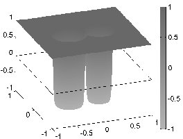
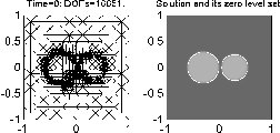
Fig. 1: The profile of $u_{0}$ and its zero level set of Test 1

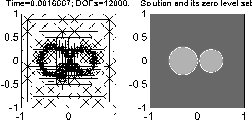
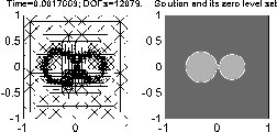
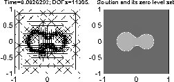
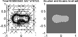
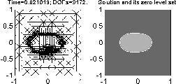
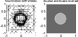
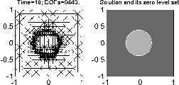
Fig. 2: Snapshots of computed solutions and adaptive meshes for Test 1

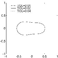
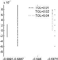
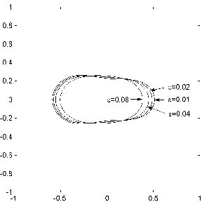
(a)                                  (b)                                  (c)

Fig. 3: Convergence of numerical interface for Test 1.

Test 2: Consider the Cahn-Hilliard equation (1)-(3) with the initial condition

(106) $$\begin{split}u_{0}(x,y)=&\tanh\bigl{(}((x-0.3)^{2}+y^{2}-0.2^{2})/{\varepsilon}\bigr{)}\tanh\bigl{(}((x+0.3)^{2}+y^{2}-0.2^{2})/{\varepsilon}\bigr{)}\times\\ &\tanh\bigl{(}(x^{2}+(y-0.3)^{2}-0.2^{2})/{\varepsilon}\bigr{)}\tanh\bigl{(}(x^{2}+(y+0.3)^{2}-0.2^{2})/{\varepsilon}\bigr{)}.\end{split}$$

Figure 4 displays the graph of the initial function $u_{0}$ and its zero level set, which encloses four circles with radius $0.2$. It also shows the initial mesh and computed initial zero level set $\Gamma_{0}^{0.01,h}$. Figure 5 shows snapshots of the solution (and its zero level set) of the Cahn-Hilliard equation and the (adaptive) mesh on which the solution is computed at $15$ different time steps. ${\varepsilon}=0.01$ and $TOL=0.02$ are used in the simulation. As expected, the fine mesh follows the zero level set as it moves. We also note that the number of elements in the initial mesh $\mathcal{T}_{0}$ is $2520$, the minimum area of the elements is $1.2207\times 10^{-4}$. If a uniform mesh is used, we need $\frac{4}{1.2207}\times 10^{4}\approx 32,768$ elements and about $148,000$ DOFs.

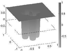
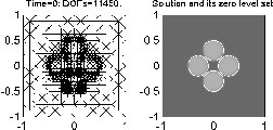
Fig. 4: The profile of $u_{0}$ and its zero level set of Test 2

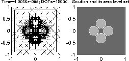
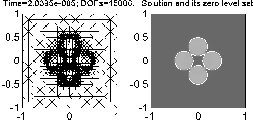
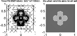
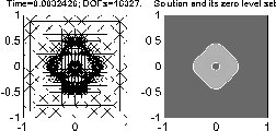
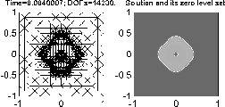
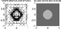
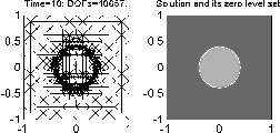
Fig. 5: Snapshots of computed solutions and adaptive meshes for Test 2

Test 3: Consider the Cahn-Hilliard equation (1)-(3) with the following initial condition

(107) $$\begin{split}u_{0}&(x,y)=\tanh\bigl{(}(x^{2}+y^{2}-0.15^{2})/{\varepsilon}\bigr{)}\times\\ &\tanh\bigl{(}((x-0.31)^{2}+y^{2}-0.15^{2})/{\varepsilon}\bigr{)}\tanh\bigl{(}((x+0.31)^{2}+y^{2}-0.15^{2})/{\varepsilon}\bigr{)}\times\\ &\tanh\bigl{(}(x^{2}+(y-0.31)^{2}-0.15^{2})/{\varepsilon}\bigr{)}\tanh\bigl{(}(x^{2}+(y+0.31)^{2}-0.15^{2})/{\varepsilon}\bigr{)}\times\\ &\tanh\bigl{(}((x-0.31)^{2}+(y-0.31)^{2}-0.15^{2})/{\varepsilon}\bigr{)}\times\\ &\tanh\bigl{(}((x-0.31)^{2}+(y+0.31)^{2}-0.15^{2})/{\varepsilon}\bigr{)}\times\\ &\tanh\bigl{(}((x+0.31)^{2}+(y-0.31)^{2}-0.15^{2})/{\varepsilon}\bigr{)}\times\\ &\tanh\bigl{(}((x+0.31)^{2}+(y+0.31)^{2}-0.15^{2})/{\varepsilon}\bigr{)}.\end{split}$$

Figure 6 displays the graph of the initial function $u_{0}$ and its zero level set, which encloses nine circles with radius $0.15$. It also shows the initial mesh and computed initial zero level set $\Gamma_{0}^{0.01,h}$. Figure 7 shows snapshots of the solution (and its zero level set) of the Cahn-Hilliard equation and the (adaptive) mesh on which the solution is computed at $15$ different time steps. ${\varepsilon}=0.01$ and $TOL=0.02$ are used in the simulation. As expected, the fine mesh follows the zero level set as it moves. We also note that the number of elements in the initial mesh $\mathcal{T}_{0}$ is $4,072$, the minimum area of the elements is $3.0518\times 10^{-5}$. If a uniform mesh is used, we need $\frac{4}{3.0518}\times 10^{5}\approx 131,072$ elements and about $590,000$ DOFs.

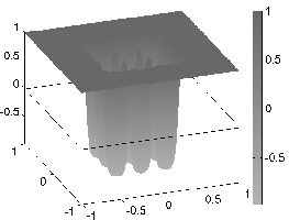
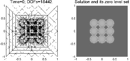
Fig. 6: The profile of $u_{0}$ and its zero level set of Test 3

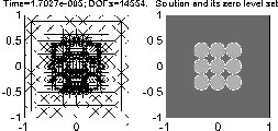
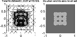
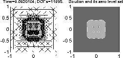
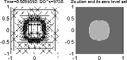
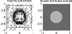
Fig. 7: Snapshots of computed solutions and adaptive meshes for Test 3

References

[1]
S. Adjerid and J. E. Flaherty.
Second-order finite element approximations and a posteriori error
estimation for two-dimensional parabolic systems.
Numer. Math., 53(1-2):183–198, 1988.
[2]
N. D. Alikakos, P. W. Bates, and X. Chen.
Convergence of the Cahn-Hilliard equation to the Hele-Shaw
model.
Arch. Rational Mech. Anal., 128(2):165–205, 1994.
[3]
N. D. Alikakos and G. Fusco.
The spectrum of the Cahn-Hilliard operator for generic interface
in higher space dimensions.
Indiana Univ. Math. J., 42(2):637–674, 1993.
[4]
S. Allen and J. W. Cahn.
A microscopic theory for antiphase boundary motion and its
application to antiphase domain coarsening.
Acta Metall., 27:1084–1095, 1979.
[5]
I. Babuška, M. Feistauer, and P. Šolín.
On one approach to a posteriori error estimates for evolution
problems solved by the method of lines.
Numer. Math., 89(2):225–256, 2001.
[6]
J. W. Barrett, J. F. Blowey, and H. Garcke.
On fully practical finite element approximations of degenerate
Cahn-Hilliard systems.
M2AN Math. Model. Numer. Anal., 35(4):713–748, 2001.
[7]
P. W. Bates and P. C. Fife.
The dynamics of nucleation for the Cahn-Hilliard equation.
SIAM J. Appl. Math., 53(4):990–1008, 1993.
[8]
S. C. Brenner and L. R. Scott.
The mathematical theory of finite element methods.
Springer-Verlag, New York, 1994.
[9]
L. A. Caffarelli and N. E. Muler.
An bound for solutions of the Cahn-Hilliard
equation.
Arch. Rational Mech. Anal., 133(2):129–144, 1995.
[10]
G. Caginalp.
An analysis of a phase field model of a free boundary.
Arch. Rational Mech. Anal., 92(3):205–245, 1986.
[11]
J. W. Cahn and J. E. Hilliard.
Free energy of a nonuniform system I. Interfacial free energy.
J. Chem. Phys., 28:258–267, 1958.
[12]
X. Chen.
Spectrum for the Allen-Cahn, Cahn-Hilliard, and phase-field
equations for generic interfaces.
Comm. Partial Differential Equations, 19(7-8):1371–1395, 1994.
[13]
X. Chen.
Global asymptotic limit of solutions of the Cahn-Hilliard
equation.
J. Differential Geom., 44(2):262–311, 1996.
[14]
G. Caginalp and X. Chen.
Convergence of the phase field model to its sharp interface limits.
European J. Appl. Math., 9(4):417–445, 1998.
[15]
P. G. Ciarlet.
The finite element method for elliptic problems.
North-Holland Publishing Co., Amsterdam, 1978.
Studies in Mathematics and its Applications, Vol. 4.
[16]
B. Cockburn.
Continuous dependence and error estimation for viscosity methods.
Acta Numerica, 12:127–180, 2003.
[17]
Q. Du and R. A. Nicolaides.
Numerical analysis of a continuum model of phase transition.
SIAM J. Numer. Anal., 28(5):1310–1322, 1991.
[18]
C. M. Elliott and D. A. French.
A nonconforming finite-element method for the two-dimensional
Cahn-Hilliard equation.
SIAM J. Numer. Anal., 26(4):884–903, 1989.
[19]
C. M. Elliott, D. A. French, and F. A. Milner.
A second order splitting method for the Cahn-Hilliard equation.
Numer. Math., 54(5):575–590, 1989.
[20]
C. M. Elliott and Z. Songmu.
On the Cahn-Hilliard equation.
Arch. Rational Mech. Anal., 96(4):339–357, 1986.
[21]
K. Eriksson and C. Johnson.
Adaptive finite element methods for parabolic problems. IV.
Nonlinear problems.
SIAM J. Numer. Anal., 32(6):1729–1749, 1995.
[22]
X. Feng.
Fully discrete finite element approximations
of the Navier-Stokes-Cahn-Hilliard diffuse interface model for
two-phase fluid flows,
SIAM J. Numer. Anal., 44:1049–1072, 2006
[23] X. Feng and O. A. Karakashian.
Fully discrete dynamic mesh discontinuous Galerkin methods for
the Cahn-Hilliard equation of phase transition.
Math. Comp., 76:1093–1117, 2007.
[24]
X. Feng and A. Prohl.
Analysis of a fully discrete finite element method for the phase
field model and approximation of its sharp interface limits.
Math. Comp., 73:541–567, 2003.
[25]
X. Feng and A. Prohl.
Error analysis of a mixed finite element method for
the Cahn-Hilliard equation.
Numer. Math., 99:47–84, 2004.
[26]
X. Feng and A. Prohl.
Numerical analysis of the Cahn-Hilliard equation and
approximation for the Hele-Shaw problem.
Interfaces and Free Boundaries, 7:1–28, 2005.
[27]
X. Feng and H. Wu.