VLBA determination of the distance to nearby star-forming regions
I. The distance to T Tauri with 0.4% accuracy

Abstract

In this article, we present the results of a series of twelve 3.6-cm radio continuum observations of T Tau Sb, one of the companions of the famous young stellar object T Tauri. The data were collected roughly every two months between September 2003 and July 2005 with the Very Long Baseline Array (VLBA). Thanks to the remarkably accurate astrometry delivered by the VLBA, the absolute position of T Tau Sb could be measured with a precision typically better than about 100 micro-arcseconds at each of the twelve observed epochs. The trajectory of T Tau Sb on the plane of the sky could, therefore, be traced very precisely, and modeled as the superposition of the trigonometric parallax of the source and an accelerated proper motion. The best fit yields a distance to T Tau Sb of 147.6 $\pm$ 0.6 pc. The observed positions of T Tau Sb are in good agreement with recent infrared measurements, but seem to favor a somewhat longer orbital period than that recently reported by Duchêne et al. (2006) for the T Tau Sa/T Tau Sb system.

1 Introduction

To provide accurate observational constraints for pre-main sequence evolutionary models, and thereby improve our understanding of star-formation, it is crucial to measure as accurately as possible the properties (age, mass, luminosity, etc.) of individual young stars. The determination of most of these parameters, however, depends critically on the often poorly known distance to the object under consideration. While the average distance to nearby low-mass star-forming regions (e.g. Taurus or $\rho-$Ophiuchus) has been estimated to about 20% precision using indirect methods (Elias 1978a,b, Kenyon et al. 1994, Knude & Hog 1998), the line-of-sight depth of these regions is largely unknown, and accurate distances to individual objects are still missing. Even the highly successful Hipparchos mission (Perryman et al. 1997) did little to improve the situation (Bertout et al. 1999) because young stars are still heavily embedded in their parental clouds and are, therefore, faint in the optical bands observed by Hipparchos. Future space missions such as GAIA will undoubtedly have the capacity to accurately measure the trigonometric parallax of optically fainter stars, but these missions will still be unable to access very deeply embedded sources, and will only start to provide results in about a decade. In the meantime, extremely high quality infrared and X-ray surveys of many star-forming regions are being obtained (e.g. Evans et al. 2003, Güdel et al. 2007), and their potential cannot be fully exploited because of the unavailability of good distance estimates.

Low-mass young stars often generate non-thermal continuum emission produced by the interaction of free electrons with the intense magnetic fields that tend to exist near their surfaces (e.g. Feigelson & Montmerle 1999). Since the magnetic field strength decreases quickly with the distance to the stellar surface (as $r^{-3}$ in the magnetic dipole approximation), the emission is strongly concentrated to the inner few stellar radii. If the magnetic field intensity and the electron energy are sufficient, the resulting compact radio emission can be detected with Very Long Baseline Interferometers (VLBI –e.g. André et al. 1992). The relatively recent possibility of accurately calibrating the phase of VLBI observations of faint, compact radio sources using nearby quasars makes it possible to measure the absolute position of these objects (or, more precisely, the angular offset between them and the calibrating quasar) to better than a tenth of a milli-arcsecond (Loinard et al. 2005, see also below). This level of precision is sufficient to constrain the trigonometric parallax of sources within a few hundred parsecs of the Sun (in particular of nearby young stars) with a precision better than a few percents using multi-epoch VLBI observations.

Taking advantage of this situation, we have recently initiated a large project aimed at accurately measuring the trigonometric parallax of a significant sample of magnetically active young stars in nearby star-forming regions (Taurus, $\rho-$Ophiuchus, Perseus, Serpens, and Cepheus) using the 10-element Very Long Baseline Array (VLBA) of the National Radio Astronomy Observatory (NRAO). In the present article, we will concentrate on T Tau Sb, one of the members of the famous young stellar system T Tauri (see e.g. Duchêne et al. 2006 for a recent summary of the properties of that system). T Tau Sb has long been known to be associated with a compact non-thermal radio source (Skinner & Brown 1994; Phillips et al. 1993, Johnston et al. 2003) characterized by strong variability and significant circular polarization. An extended, thermal, radio halo studied in detail by Loinard et al. (2007) and probably related to stellar winds, also exist around T Tau Sb. While this extended structure contributes to the total radio flux as measured, for instance, with the VLA, it is effectively filtered out in Very Long Baseline Interferometry experiments. Indeed, in the intercontinental VLBI observations published by Smith et al. (2003), only about 40% of the simultaneously measured VLA flux density is retrieved. The radio source detected by Smith et al. (2003) is very compact (R $<$ 15 R_⊙), and its flux was about 3 mJy at the time of their observations. Its trajectory over the plane of the sky was studied by Loinard et al. (2005) using a series of 7 VLBA observations. Unfortunately, these data were recently found to have been affected by a bug that caused the VLBA correlator to use predicted rather than measured Earth Orientation Parameters (see http://www.vlba.nrao.edu/astro/messages/eop/). This problem corrupted the visibility phases, and strongly affected the quality of the astrometry of the data published in Loinard et al. (2005). The post-fit rms for the data published by Loinard et al. (2005) was about 250 mas compared with 60–90 mas for the present data (see below). Here, we will re-analyze these VLBA data, and combine them with 5 newer observations to measure the trigonometric parallax, and study the proper motion of T Tau Sb.

2 Observations and data calibration

In this paper, we will make use of a series of twelve continuum 3.6 cm (8.42 GHz) observations of T Tau Sb obtained every two months between September 2003 and July 2005 with the VLBA (Tab. 1). Our phase center was at $\alpha_{J2000.0}$ = $04^{\rm h}21^{\rm m}59\mbox{${}^{\rm s}\mskip-7.6mu.\,$}4263$, $\delta_{J2000.0}$ = +$19^{\circ}32^{\prime}05\mbox{${}^{\prime\prime}\mskip-7.6mu.\,$}730$, the position of the compact source detected by Smith et al. (2003). Each observation consisted of series of cycles with two minutes spent on source, and one minute spent on the main phase-referencing quasar J0428+1732, located $2\mbox{${}^{\circ}\mskip-7.6mu.\,$}6$ away. J0428+1732 is a very compact extragalactic source whose absolute position ($\alpha_{J2000.0}$ = $04^{\rm h}28^{\rm m}35\mbox{${}^{\rm s}\mskip-7.6mu.\,$}633679$,$\delta_{J2000.0}$ = $17^{\circ}32^{\prime}23\mbox{${}^{\prime\prime}\mskip-7.6mu.\,$}58799$) is known to better than 1 milli-arcsecond ($\sigma_{\alpha}$ = 0.59 mas, $\sigma_{\delta}$ = 0.89 mas; Beasley et al. 2002). During the first 6 observations, the secondary quasar J0431+1731 was also observed periodically –about every 30 minutes– to check the astrometric quality of the data, and to compare our results with those of Smith et al. (2003) who used J0431+1731 as their phase calibrator. A detailed comparison with the results of Smith et al. (2003) and with the numerous VLA observations available from the literature, however, will be postponed to a forthcoming article.

The data were edited and calibrated using the Astronomical Image Processing System (AIPS –Greisen 2003). The basic data reduction followed the standard VLBA procedures for phase-referenced observations. First, the most accurate measured Earth Orientation Parameters obtained from the US Naval Observatory database were applied to the data in order to correct the erroneous values initially used by the VLBA correlator. Second, dispersive delays caused by free electrons in the Earth’s atmosphere were accounted for using estimate of the electron content of the ionosphere derived from Global Positioning System (GPS) measurements. A priori amplitude calibration based on the measured system temperatures and standard gain curves was then applied. The fourth step was to correct the phases for antenna parallactic angle effects, and the fifth was to remove residual instrumental delays caused by the VLBA electronics. This was done by measuring the delays and phase residuals for each antenna and IF using the fringes obtained on a strong calibrator. The final step of this initial calibration was to remove global frequency- and time-dependent phase errors using a global fringe fitting procedure on the main phase calibrator (J0428+1732), which was assumed at this stage to be a point source.

In this initial calibration, the solutions from the global fringe fit were only applied to the main phase calibrator itself. The corresponding calibrated visibilities were then imaged, and several passes of self-calibration were performed to improve the overall amplitude and phase calibration. In the image obtained after the self-calibration iterations, the main phase calibrator is found to be slightly extended. To take this into account, the final global fringe fitting part of the reduction was repeated using the image of the main phase calibrator as a model instead of assuming it to be a point source. Note that a different phase calibrator model was produced for each epoch to account for possible small changes in the main calibrator structure from epoch to epoch. The solutions obtained after repeating this final step were edited for bad points and applied to the target source. Using an image model for the calibrator rather than assuming a point source improved the position accuracy by a few tens of $\mu$as.

Because of the significant overheads that were necessary to properly calibrate the data, only about 3 of the 6 hours of telescope time allocated to each of our observations were actually spent on source. Once calibrated, the visibilities were imaged with a pixel size of 50 $\mu$as after weights intermediate between natural and uniform (ROBUST = 0 in AIPS) were applied. This resulted in a typical r.m.s. noise level of 70 $\mu$Jy for most observations, though for a few epochs with less favorable weather conditions, the noise level exceeded 100 $\mu$Jy (Tab. 1). T Tau Sb was detected with a signal to noise better than 10 at each epoch (Tab. 1), and its absolute position (listed in columns 2 and 4 of Tab. 1) was determined using a 2D Gaussian fitting procedure (task JMFIT in AIPS). This task provides an estimate of the position error (columns 3 and 5 of Tab. 1) based on the expected theoretical astrometric precision of an interferometer (Condon 1997). Systematic errors, however, usually limit the actual precision of VLBI astrometry to several times this theoretical value (e.g. Fomalont et al. 1999, Pradel et al. 2006). At the frequency of the present observations, the main sources of systematic errors are inaccuracies in the troposphere model used, as well as clock, antenna and a priori source position errors. These effects combine to produce a systematic phase difference between the calibrator and the target that limits the precision with which the target position can be determined. We did not attempt to correct for these systematic effects here, and will, therefore, assume that the true error on each measurement is the quadratic sum of the random error listed in Tab. 1 and a systematic contribution. The latter is difficult to estimate a priori, and will be deduced from the fits to the data.

3 Astrometry fits

The displacement of T Tau Sb on the celestial sphere is the combination of its trigonometric parallax ($\pi$) and its proper motion. For isolated sources, it is common to consider linear and uniform proper motions, so the right ascension ($\alpha$) and the declination ($\delta$) vary as a function of time $t$ as:

$$\alpha(t) = \alpha_{0}+(\mu_{\alpha}\cos\delta)t+\pi f_{\alpha}(t)$$ (1)

$$\delta(t) = \delta_{0}+\mu_{\delta}t+\pi f_{\delta}(t),$$ (2)

where $\alpha_{0}$ and $\delta_{0}$ are the coordinates of the source at a given reference epoch, $\mu_{\alpha}$ and $\mu_{\delta}$ are the components of the proper motion, and $f_{\alpha}$ and $f_{\delta}$ are the projections over $\alpha$ and $\delta$, respectively, of the parallactic ellipse. The latter functions are given by (e.g. Seidelman 1992):

$$f_{\alpha}(t) = (X\sin\alpha_{1}-Y\cos\alpha_{1})/(15\cos\delta_{1})$$ (3)

$$f_{\delta}(t) = (X\cos\alpha_{1}\sin\delta_{1}+Y\sin\alpha_{1}\sin\delta_{1}-Z\cos\delta_{1}),$$ (4)

where (X,Y,Z) are the barycentric coordinates of the Earth in Astronomical Units, and where $\alpha_{1}$ = $\alpha-\pi f_{\alpha}(t)$ and $\delta_{1}$ = $\delta-\pi f_{\delta}(t)$ are the coordinates of the barycentric place of the source at each epoch. Note that $f_{\alpha}$ and $f_{\delta}$ depend implicitly on time (through X,Y,Z) and explicitly on the coordinates of the source. The latter dependence on $\alpha_{1}$ and $\delta_{1}$ (which are only known if the trigonometric parallax is known) implies that the fitting procedure must be iterative. The barycentric coordinates of the Earth (as well as the Julian Date of each observation) were calculated using the Multi-year Interactive Computer Almanac (MICA) distributed as a CDROM by the US Naval Observatory. They are given explicitly in Tab. 2 for all epochs.

Figure 1: Measured positions of T Tau Sb and best fit without (a) and with (b) acceleration terms. The observed positions are shown as ellipses, the size of which represents the magnitude of the errors. Note the very significant improvement when acceleration terms are included.

As mentioned earlier, T Tau Sb is a member of a multiple system (e.g. Loinard et al. 2003, Duchêne et al. 2006 and references therein), so its proper motion is likely to be affected by the gravitational influence of the other members of the system. As a consequence, the motion is likely to be curved and accelerated, rather than linear and uniform. To take this into account, we have also made fits to the data that include acceleration terms. This leads to functions of the form:

$$\alpha(t) = \alpha_{0}+(\mu_{\alpha 0}\cos\delta)t+{1\over 2}(a_{\alpha}\cos\delta)t^{2}+\pi f_{\alpha}(t)$$ (5)

$$\delta(t) = \delta_{0}+\mu_{\delta 0}t+{1\over 2}a_{\delta}t^{2}+\pi f_{\delta}(t),$$ (6)

where $\mu_{\alpha 0}$ and $\mu_{\delta 0}$ are the proper motions at a reference epoch, and $a_{\alpha}$ and $a_{\delta}$ are the projections of the uniform acceleration. Note that the acceleration undergone by a body in Keplerian orbit is usually not uniform. Assuming a uniform acceleration is acceptable here, however, because our data cover only a small portion ($\sim$ 2 yr) of the orbital period (a few decades –Duchêne et al. 2006) of T Tau Sb. If VLBA data are obtained regularly in the next few decades, a full orbital fit will become possible, and indeed, necessary.

The astrometric parameters were determined by least-square fitting the data points with either Eqs. 1–2 or Eqs. 5–6 using a Singular Value Decomposition (SVD) scheme (see Appendix for details). To check our results, we also performed two other fits to the data, a linear one based on the associated normal equations, and a non-linear one based on the Levenberg-Marquardt algorithm. They gave results identical to those obtained using the SVD method. The reference epoch was taken at the mean of our observations (JD 2453233.586 $\equiv$ J2004.627).

4 Results

The fit to the data points by Eqs. 1–2 (Fig. 1a) yields the following astrometric parameters:

$$\alpha_{J2004.627} = \mbox{ $04^{\rm h}21^{\rm m}59\mbox{${}^{\rm s}\mskip-7.6mu.\,$}425081$ }~{}\pm~{}\mbox{ $0\mbox{${}^{s}\mskip-7.6mu.\,$}000005$ }$$

$$\delta_{J2004.627} = \mbox{ $19^{\circ}32^{\prime}05\mbox{${}^{\prime\prime}\mskip-7.6mu.\,$}71566$ }~{}\pm~{}\mbox{ $0\mbox{${}^{\prime\prime}\mskip-7.6mu.\,$}00003$ }$$

$$\mu_{\alpha}\cos\delta = 4.00~{}\pm~{}0.12~{}\mbox{mas yr${}^{-1}$}$$

$$\mu_{\delta} = -1.18~{}\pm~{}0.05~{}\mbox{mas yr${}^{-1}$}$$

$$\pi = 6.90~{}\pm~{}0.09~{}\mbox{mas.}$$

This corresponds to a distance of 145 $\pm$ 2 pc. The post-fit rms, however, is not very good (particularly in right ascension: $\sim$ 0.2 mas) as the fit does not pass through many of the observed positions (Fig. 1a). As a matter of fact, 75 micro-arcsecond and –most notably– 16.5 microseconds of time had to be added quadratically to the formal errors listed in Tab. 1 to obtain a reduced $\chi^{2}$ of 1 in both right ascension and declination; the errors on the fitted parameters quoted above include this systematic contribution. These large systematic errors most certainly reflect the fact mentioned earlier that the proper motion of T Tau Sb is not uniform because it belongs to a multiple system. Indeed, the fit where acceleration terms are included is significantly better (Fig. 1b) with a post-fit rms of 60 $\mu$as in right ascension and 90 $\mu$as in declination. It yields the following parameters:

$$\alpha_{J2004.627} = \mbox{ $04^{\rm h}21^{\rm m}59\mbox{${}^{\rm s}\mskip-7.6mu.\,$}425065$ }~{}\pm~{}\mbox{ $0\mbox{${}^{s}\mskip-7.6mu.\,$}000002$ }$$

$$\delta_{J2004.627} = \mbox{ $19^{\circ}32^{\prime}05\mbox{${}^{\prime\prime}\mskip-7.6mu.\,$}71566$ }~{}\pm~{}\mbox{ $0\mbox{${}^{\prime\prime}\mskip-7.6mu.\,$}0004$ }$$

$$\mu_{\alpha,~{}J2004.627}\cos\delta = 4.02~{}\pm~{}0.03~{}\mbox{mas yr${}^{-1}$}$$

$$\mu_{\delta,~{}J2004.627} = -1.18~{}\pm~{}0.05~{}\mbox{mas yr${}^{-1}$}$$

$$a_{\alpha}\cos\delta = 1.53~{}\pm~{}0.13~{}\mbox{mas yr${}^{-2}$}$$

$$a_{\delta} = 0.00~{}\pm~{}0.19~{}\mbox{mas yr${}^{-2}$}$$

$$\pi = 6.82~{}\pm~{}0.03~{}\mbox{mas.}$$

To obtain a reduced $\chi^{2}$ of 1 in both right ascension and declination, one must add quadratically 3.8 microseconds of time and 75 microseconds of arc to the statistical errors listed in Tab. 1. The uncertainties reported above and in the rest of this article include this systematic contribution. Note also that the reduced $\chi^{2}$ for the fit without acceleration terms is almost 8, if the latter systematic errors (rather than those mentioned earlier) are used.

The trigonometric parallax obtained when acceleration terms are included, corresponds to a distance of 146.7 $\pm$ 0.6 pc, somewhat larger than, but consistent within 1.5$\sigma$ with the value reported by Loinard et al. (2005). Recall, however, that this 2005 result was based on data that had been corrupted by a problem in the VLBA correlator; we consider the present value significantly more reliable. The present distance determination is somewhat smaller than, but within 1$\sigma$ of the distance obtained by Hipparchos ($d$ = 177${}^{+68}_{-39}$ pc). Note that the relative error of our distance is about 0.4%, against nearly 30% for the Hipparchos result, a gain of almost two orders of magnitude.

5 Implications for the properties of the stars

Having obtained an improved distance estimate to the T Tauri system, we are now in a position to refine the determination of the intrinsic properties of each of the components of that system. Since the orbital motion between T Tau N and T Tau S is not yet known to very good precision, we will use synthetic spectra fitting to obtain the properties of T Tau N. For the very obscured T Tau S companion, on the other hand, we will refine the mass determinations based on the orbital fit obtained by Duchêne et al. (2006).

5.1 T Tau N

The stellar parameters ($T_{\mbox{eff}}$ and $L_{\mbox{bol}}$) of T Tau N were obtained by fitting synthetic spectra (Lejeune et al. 1997) to the optical part of the spectral energy distribution. In the absence of recently published optical spectra with absolute flux calibration, we decided to use narrow-band photometry taken at six different epochs from 1965 to 1970 (Kuhi 1974). In order to eliminate the contamination by the UV/blue (magnetospheric accretion) and red/IR (circumstellar disk) excesses, we restricted the fit to the range 0.41–0.65 $\mu$m. Two points at $\lambda\lambda$ 0.4340, 0.4861 $\mu$m display large variations between epochs, they were also discarded as they are likely to be contaminated by emission lines. As a consequence, 56 photometric measurements at 13 wavelengths and 6 epochs had to be fitted. (See Fig. 2). We assumed that the star kept constant intrinsic parameters over the 5 years of observation, but allowed the circumstellar extinction to vary. Such an hypothesis is supported by long-term photometric observations (1986-2003) that show color-magnitude diagrams of T Tau elongated along the extinction direction (Melnikov & Grankin 2005); Kuhi (1974) also measured significant extinction variation in the period 1965-1970 using color excesses.

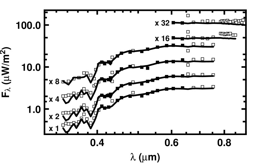
Figure 2: Fit to the photometry at six different epochs. Black squares are point that have been fitted; white squares represent other wavelengths excluded from the fit.

The non-linear fitting procedure used the Levenberg-Marquardt method and the determination of errors was done using a Monte Carlo simulation. The synthetic spectra were transformed into narrow-band photometry by integration over the bandwidth of the measurements (typically 0.05 $\mu$m). As the fitting procedure could not constrain the metallicity, we assumed a solar one. Several fits using randomly chosen initial guesses for $T_{\mbox{eff}}$, $L_{\mbox{bol}}$, and extinctions were performed in order to ensure that a global minimum $\chi^{2}$ was indeed reached. The errors reported by Kuhi (1974; 1.2%) had to be renormalised to 5.9% in order to achieve a reduced $\chi^{2}$ of 1. This could result from an underestimation by the author or from positive and negative contamination by spectral lines –indeed, Gahm (1970) reports contamination as high as 20% for RW Aur. The best least-squares fit is represented in Fig. 3, and yields $T_{\mbox{eff}}=5112_{-97}^{+99}$ K and $L_{\mbox{bol}}=5.11_{-0.66}^{+0.76}\,L_{\odot}$. The extinction varies between 1.02 and 1.34, within 1-$\sigma$ of the values determined by Kuhi (1974) from color excesses. The effective temperature is consistent with a K1 star as reported by Kuhi (1974).

In order to derive the age and mass of T Tau N, pre-main-sequence isochrones by D’Antona & Mazzitelli (1996) and Siess et al. (2000) were used. The fitting procedure was identical to the previous one: the age and mass were converted into effective temperature and luminosity, which in turn were converted into narrow-band photometry using the synthetic spectra. The derived parameters are shown in Tab. 3. The masses (1.83${}^{+0.20}_{-0.16}$ and 2.14${}^{+0.11}_{-0.10}$ M_⊙) have overlapping error bars and are consistent with values found in the literature (e.g Duchêne et al. 2006). The predicted ages, on the other hand, differ by a factor of 2. While the isochrones by D’Antona & Mazzitelli (1996) give an age in the commonly accepted range ($1.15^{+0.18}_{-0.16}$ Myr), a somewhat larger value ($2.39^{+0.31}_{-0.27}$) is derived from Siess et al. (2000). Note that the errors on the derived parameters are entirely dominated by the modeling errors; the uncertainty on the distance now represents a very small fraction of the error budget.

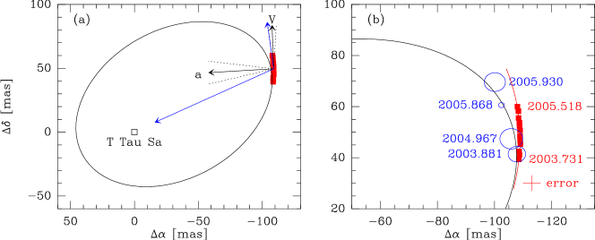
Figure 3: (a) VLBA positions (red squares) registered to T Tau Sa overimposed on the elliptical fit proposed by Duchêne et al. (2006). Also shown are the velocity and acceleration vectors for our mean epoch deduced from our observations, as well as their counterparts from the fit by Duchêne et al. (shown in blue). The dotted black lines around the measured acceleration and velocity show the error cone on the direction of each of these vectors. (b) Zoom on the region corresponding to our observations. In addition to the orbit and the VLBA positions, we show (in red) our best parabolic fit to our positions, as well as several recent infrared positions (in blue). The 2003.881 position is from Duchêne et al. (2005), the 2004.967 and 2005.868 positions are from Duchêne et al. (2006), and the 2005.930 position is from Schaefer et al. (2006).

5.2 T Tau S

The two members of the T Tau S system have been studied in detail by Duchêne and coworkers in a series of recent articles (Duchêne et al. 2002, 2005, 2006). The most massive member of the system (T Tau Sa) belongs to the mysterious class of “infrared companions”, and is presumably the precursor of an intermediate-mass star. T Tau Sb, on the other hand is a very obscured, but otherwise normal, pre-main sequence M1 star. The mass of both T Tau Sa and T Tau Sb were estimated by Duchêne et al. (2006) using a fit to their orbital paths. Those authors used the distance to T Tauri deduced from Loinard et al. (2005). Using the new distance determination obtained here, we can re-normalize those masses. We obtain $M_{Sa}$ = 3.10 $\pm$ 0.34 M_⊙, and $M_{Sb}$ = 0.69 $\pm$ 0.18 M_⊙. These values may need to be adjusted somewhat, however, as the fit to the orbital path of the T Tau Sa/T Tau Sb system is improved (see below). Note finally, that the main sources of errors on the masses are related to the orbital motion modeling rather than to the uncertainties of the distance.

6 Implications for the orbital motions

T Tau Sb is a member of a multiple system, so it would be desirable to give its position and express its motion relative to the other members of the system, T Tau N and –particularly– T Tau Sa. Since only T Tau Sb is detected in our VLBA observations, however, registering the positions reported here to the other members of the system involves a number of steps. The absolute position and proper motion of T Tau N has been measured to great precision using over 20 years of VLA observations (Loinard et al. 2003), so registering the position and motion of T Tau Sb relative to T Tau N is fairly straightforward. Combining the data used by Loinard et al. (2003) with several more recent VLA observations, we obtained the following absolute position (at epoch J2000.0) and proper motion for T Tau N:

$$\alpha_{J2000.0} = \mbox{ $04^{\rm h}21^{\rm m}59\mbox{${}^{\rm s}\mskip-7.6mu.\,$}4321$ }~{}\pm~{}\mbox{ $0\mbox{${}^{s}\mskip-7.6mu.\,$}0001$ }$$

$$\delta_{J2000.0} = \mbox{ $19^{\circ}32^{\prime}06\mbox{${}^{\prime\prime}\mskip-7.6mu.\,$}419$ }~{}\pm~{}\mbox{ $0\mbox{${}^{\prime\prime}\mskip-7.6mu.\,$}002$ }$$

$$\mu_{\alpha}\cos\delta = 12.35~{}\pm~{}0.04~{}\mbox{mas yr${}^{-1}$}$$

$$\mu_{\delta} = -12.80~{}\pm~{}0.06~{}\mbox{mas yr${}^{-1}$.}$$

Subtracting these values from the absolute positions and proper motion of T Tau Sb, we can obtain the positional offset between T Tau Sb and T Tau N, as well as their relative proper motion. For the median epoch of our observations, we obtain:

$$\mu_{\alpha}\cos\delta\mbox{(Sb/N)} = -8.33~{}\pm~{}0.07~{}\mbox{mas yr${}^{-1}$}$$

$$\mu_{\delta}\mbox{(Sb/N)} = +11.62~{}\pm~{}0.11~{}\mbox{mas yr${}^{-1}$}.$$

The second step consists in registering the position and motion of T Tau Sb to the center of mass of T Tau S using the parabolic fits provided by Duchêne et al. (2006). Here, both the proper motion and the acceleration must be taken into account. For the mean epoch of our observations, we obtain:

$$\mu_{\alpha}\cos\delta\mbox{(Sb/CM)} = +0.3~{}\pm~{}0.9~{}\mbox{mas yr${}^{-1}$}$$

$$\mu_{\delta}\mbox{(Sb/CM)} = +9.3~{}\pm~{}0.8~{}\mbox{mas yr${}^{-1}$}$$

$$a_{\alpha}\cos\delta\mbox{(Sb/CM)} = +1.4~{}\pm~{}0.2~{}\mbox{mas yr${}^{-2}$}$$

$$a_{\delta}\mbox{(Sb/CM)} = -0.1~{}\pm~{}0.3~{}\mbox{mas yr${}^{-2}$}.$$

The last correction to be made is the registration of the positions, proper motions, and accelerations to T Tau Sa rather than to the center of mass of T Tau S. This is obtained by simply multiplying the values above by the ratio of the total mass of T Tau S (i.e. $M_{Sa}$+$M_{Sb}$) to the mass of Sa. Using the masses given by Duchêne et al. 2006), we obtain:

$$\mu_{\alpha}\cos\delta\mbox{(Sb/Sa)} = +0.4~{}\pm~{}1.1~{}\mbox{mas yr${}^{-1}$}$$

$$\mu_{\delta}\mbox{(Sb/Sa)} = +11.4~{}\pm~{}1.0~{}\mbox{mas yr${}^{-1}$}$$

$$a_{\alpha}\cos\delta\mbox{(Sb/Sa)} = +1.7~{}\pm~{}0.2~{}\mbox{mas yr${}^{-2}$}$$

$$a_{\delta}\mbox{(Sb/Sa)} = -0.1~{}\pm~{}0.3~{}\mbox{mas yr${}^{-2}$}.$$

These two vectors are shown in Fig. 3 together with the VLBA positions registered to T Tau Sa, several recent infrared observations and the elliptical fit obtained by Duchêne et al. (2006). The final error on the VLBA positions is the combination of the original uncertainty on their measured absolute position, and of the errors made at each of the steps described above. The final uncertainty is about 3 mas in both right ascension and declination, and is shown near the bottom right corner of Fig. 3b.

Given the uncertainties, the position of the VLBA source is generally in good agreement with the infrared source position measured at similar epochs. Indeed, the first 2 VLBA observations were obtained almost exactly at the same time as the infrared image published by Duchêne et al. (2005), and the positions match exactly. The position of the VLBA source at the end of 2004 is also in agreement within 1$\sigma$ with the position of the infrared source at the same epoch reported by Duchêne et al. (2006). The situation at the end of 2005, however, is somewhat less clear. Extrapolating from the last VLBA observation ($\sim$ 2005.5) to the end of 2005 gives a location that would be in reasonable agreement with the position given by Schaefer et al. (2006) but clearly not with the position obtained by Duchêne et al. (2006). Note, indeed, that the two infrared positions are only very marginally consistent with one another.

Our VLBA observations suggest that T Tau Sb passed at the westernmost point of its orbit around 2005.0, whereas according to the fit proposed by Duchêne et al. (2006), this westernmost position was reached slightly before 2004.0. As a consequence, the trajectory described by the VLBA source is on average almost exactly north-south, whereas according to the fit proposed by Duchêne et al. (2006), T Tau Sb is already moving back toward the east (Fig. 3). We note, however, that the fit proposed by Duchêne et al. (2006, which gives an orbital period of 21.7 $\pm$ 0.9 yr) is very strongly constrained by their 2005.9 observation. Shaefer et al. (2006), who measured a position at the end of 2005 somewhat more to the north (in better agreement with our VLBA positions), argue that they cannot discriminate between orbital periods of 20, 30 or 40 yr. Orbits with longer periods bend back toward the east somewhat later (see Fig. 10 in Schaefer et al. 2006), and would be in better agreement with our VLBA positions.

Another element that favors a somewhat longer orbital period is the acceleration measured here. According to the fit proposed by Duchêne et al. (2006), the expected transverse proper motion and acceleration are (G. Duchêne, private communication):

$$\mu_{\alpha}\cos\delta\mbox{(Sb/Sa)} = +1.7~{}\pm~{}0.2~{}\mbox{mas yr${}^{-1}$}$$

$$\mu_{\delta}\mbox{(Sb/Sa)} = +12.1~{}\pm~{}1.2~{}\mbox{mas yr${}^{-1}$}.$$

$$a_{\alpha}\cos\delta\mbox{(Sb/Sa)} = +3.1~{}\pm~{}0.5~{}\mbox{mas yr${}^{-2}$}$$

$$a_{\delta}\mbox{(Sb/Sa)} = -1.4~{}\pm~{}0.2~{}\mbox{mas yr${}^{-2}$}.$$

Thus, while the expected and observed proper motions are in good agreement, the expected acceleration is significantly larger that the observed value (see also Fig. 3). A smaller value of the acceleration would be consistent with a somewhat longer orbital period.

In summary, our observations appear to be in reasonable agreement with all the published infrared positions obtained over the last few years, except for the 2005.9 observation reported by Duchêne et al. (2006). As a consequence, our data favor an orbital period somewhat longer than that obtained by Duchêne et al. (2006). Exactly how much longer is difficult to assess for the following reason. The orbit proposed by Duchêne et al. (2006) was obtained by fitting simultaneously the observed positions with a superposition of an elliptical path (of Sb around Sa) and a parabolic trajectory (of Sa around N). As a consequence, a modification of the Sa/Sb elliptical orbit (as may be required by our data) will result in a change in the parameters of the parabolic fit. But we use the latter to register our VLBA positions, proper motions, and accelerations against T Tau Sa. Thus, an entirely new fit will be needed to take into account the present VLBA observations. Such a fit will be presented in a forthcoming paper, where the numerous VLA observations available from the literature, as well as the VLBI observation from Smith et al. (2003) will also be taken into account.

7 Conclusions and perspectives

Using a series of 12 radio-continuum VLBA observations of T Tau Sb obtained roughly every two months between September 2003 and July 2005, we have measured the trigonometric parallax and characterized the proper motion of this member of the T Tauri multiple system with unprecedented accuracy. The distance to T Tau Sb was found to be 146.7 $\pm$ 0.6 pc, somewhat larger than the canonical value of 140 pc traditionally used. Using this precise estimate, we have recalculated the basic parameters of all three members of the system. The VLBA positions are in good agreement with recent infrared positions, but our data seem to favor a somewhat longer orbital period than that recently reported by Duchêne et al. (2006) for the T Tau Sa/T Tau Sb system.

Finally, it should be pointed out that if observations similar to those presented here were obtained regularly in the coming 5 to 10 years, they would greatly help to constrain the orbital path (and, therefore, the mass) of the T Tau Sa/T Tau Sb system.

Appendix A Appendix

The parameters determined in this article (position at a reference epoch, trigonometric parallax, proper motions and accelerations) were obtained by minimizing the sum ($\chi_{\alpha}^{2}+\chi_{\delta}^{2}$) of the residuals in right ascension and declination. The corresponding general mathematical problem is that where two functions $x$ and $y$ depend linearly on $N$ independent parameters ($a_{i}$ and $b_{i}$ for $x$ and $y$, respectively), and $M$ common parameters $c_{i}$:

$$x(t) = \sum_{i=1}^{N}a_{i}u_{i}(t)+\sum_{j=1}^{M}c_{j}w^{x}_{j}(t)$$

$$y(t) = \sum_{i=1}^{N}b_{i}v_{i}(t)+\sum_{j=1}^{M}c_{j}w^{y}_{j}(t)$$

The values $x_{k}$ and $y_{k}$ of the functions $x$ and $y$ have been measured at $P$ times $t_{k}$ with errors $\sigma^{x}_{k}$ and $\sigma^{y}_{k}$, respectively, and the total $\chi^{2}$ can be written:

$$\chi^{2} = \chi_{x}^{2}+\chi_{y}^{2}$$

$$= \sum_{k=1}^{P}\left(\left[{x_{k}-\left(\sum_{i=1}^{N}a_{i}u_{i}(t_{k})+\sum_{j=1}^{M}c_{j}w^{x}_{j}(t_{k})\right)\over\sigma^{x}_{k}}\right]^{2}+\left[{y_{k}-\left(\sum_{i=1}^{N}b_{i}v_{i}(t_{k})+\sum_{j=1}^{M}c_{j}w^{y}_{j}(t_{k})\right)\over\sigma^{y}_{k}}\right]^{2}\right)$$

Defining the following matrix elements:

$$\alpha_{ki} = {u_{i}(t_{k})\over\sigma_{k}^{x}}$$

$$\beta_{ki} = {v_{i}(t_{k})\over\sigma_{k}^{y}}$$

$$\gamma_{kj} = {w_{j}^{x}(t_{k})\over\sigma_{k}^{x}}$$

$$\delta_{kj} = {w_{j}^{y}(t_{k})\over\sigma_{k}^{y}}$$

$$\theta_{k} = {x_{k}\over\sigma_{k}^{x}}$$

$$\psi_{k} = {y_{k}\over\sigma_{k}^{y}},$$

we can re-write the total $\chi^{2}$ given by equation LABEL:chi2 as:

$$\chi^{2} = \sum_{k=1}^{P}\left(\left[\theta_{k}-\sum_{i=1}^{N}\alpha_{ki}a_{i}-\sum_{j=1}^{M}\gamma_{kj}c_{j}\right]^{2}+\left[\psi_{k}-\sum_{i=1}^{N}\beta_{ki}b_{i}-\sum_{j=1}^{M}\delta_{kj}c_{j}\right]^{2}\right)$$

This sum of quadratic terms can clearly be seen as the squared norm of the vector:

$$\left(\begin{array}[]{c}\theta_{1}-\sum_{i=1}^{N}\alpha_{1i}a_{i}-\sum_{j=1}^{M}\gamma_{1j}c_{j}\\ \theta_{2}-\sum_{i=1}^{N}\alpha_{2i}a_{i}-\sum_{j=1}^{M}\gamma_{2j}c_{j}\\ \dotfill\hfil\\ \theta_{P}-\sum_{i=1}^{N}\alpha_{Pi}a_{i}-\sum_{j=1}^{M}\gamma_{Pj}c_{j}\\ \psi_{1}-\sum_{i=1}^{N}\beta_{1i}b_{i}-\sum_{j=1}^{M}\delta_{1j}c_{j}\\ \psi_{2}-\sum_{i=1}^{N}\beta_{2i}b_{i}-\sum_{j=1}^{M}\delta_{2j}c_{j}\\ \dotfill\hfil\\ \psi_{P}-\sum_{i=1}^{N}\beta_{Pi}b_{i}-\sum_{j=1}^{M}\delta_{Pj}c_{j}\\ \end{array}\right)$$

Re-arranging the terms in this expression, we can re-write the total $\chi^{2}$ as:

$$\chi^{2}=\left|\left|\left(\begin{array}[]{ccc}\alpha&0&\gamma\\ 0&\beta&\delta\end{array}\right)\left(\begin{array}[]{c}a\\ b\\ c\end{array}\right)-\left(\begin{array}[]{c}\theta\\ \psi\end{array}\right)\right|\right|^{2}$$ (A2)

The procedure then consists of finding the vector $\mathbf{X}$ that minimizes an expression of the form:

$$\left|\left|A.X-B\right|\right|^{2}$$

An efficient algorithm to perform this operation is known as the Singular Value Decomposition (SVD –see Press et al. 1992). This method is based on the linear algebra theorem that states that any $I\times J$ rectangular matrix $\mathbf{M}$ whose number $I$ of rows is larger or equal to its number $J$ of columns, can written as the product of an $I\times J$ column-orthogonal matrix $\mathbf{U}$ by a $J\times J$ diagonal matrix $\mathbf{W}$ with positive or zero elements, and the transpose of a $J\times J$ orthogonal matrix $\mathbf{V}$:

$$M=U~{}W~{}V^{T}$$ (A3)

The rectangular matrix in expression A2 has $2P$ rows (=24 in our case) and $2N+M$ column (=5 or 7, for uniform or accelerated proper motions, respectively) and can clearly be decomposed in that fashion. Since both $\mathbf{U}$ and $\mathbf{V}$ in the previous expression are orthogonal, their inverses are just their transposes. Also, if none of its diagonal elements are zero (which will be the case in all situations considered here), the inverse of $\mathbf{W}$ is a diagonal matrix whose elements are just the inverses of those of $\mathbf{W}$. Thus, the inverse of matrix $\mathbf{M}$ can be written as:

$$M^{-1}=V~{}W^{-1}~{}U^{T}$$

It can be shown (see Press et al. 1992) that, if the matrix $\mathbf{M}$ can be decomposed as above, then the vector $\mathbf{X}$ that minimizes the expression $\left|\left|A.X-B\right|\right|^{2}$ is simply:

$$X=V~{}W^{-1}~{}U^{T}B$$ (A4)

An efficient way of solving our least-squares fit problem is, therefore, to form the rectangular matrix that appears in expression A2, decompose it as in A3, and calculate the value of the $a_{i}$’s, $b_{i}$’s, and $c_{i}$’s using A4. This method was implemented in FORTRAN following Press et al. (1992).

Table 1: Source position and flux

Mean UT date	$\alpha$ (J2000.0)	$\sigma_{\alpha}$	$\delta$ (J2000.0)	$\sigma_{\delta}$	$F_{\nu}$	$\sigma$
(yyyy.mm.dd    hh:mm)					(mJy)	($\mu$Jy)
2003.09.24    11:33	$04^{\rm h}21^{\rm m}59\mbox{${}^{\rm s}\mskip-7.6mu.\,$}4252942$	$0\mbox{${}^{s}\mskip-7.6mu.\,$}0000013$	$19^{\circ}32^{\prime}05\mbox{${}^{\prime\prime}\mskip-7.6mu.\,$}717618$	$0\mbox{${}^{\prime\prime}\mskip-7.6mu.\,$}000043$	1.62	74
2003.11.18    08:02	$04^{\rm h}21^{\rm m}59\mbox{${}^{\rm s}\mskip-7.6mu.\,$}4249805$	$0\mbox{${}^{s}\mskip-7.6mu.\,$}0000015$	$19^{\circ}32^{\prime}05\mbox{${}^{\prime\prime}\mskip-7.6mu.\,$}716554$	$0\mbox{${}^{\prime\prime}\mskip-7.6mu.\,$}000043$	1.74	66
2004.01.15    04:09	$04^{\rm h}21^{\rm m}59\mbox{${}^{\rm s}\mskip-7.6mu.\,$}4245823$	$0\mbox{${}^{s}\mskip-7.6mu.\,$}0000036$	$19^{\circ}32^{\prime}05\mbox{${}^{\prime\prime}\mskip-7.6mu.\,$}715322$	$0\mbox{${}^{\prime\prime}\mskip-7.6mu.\,$}000108$	0.92	72
2004.03.26    23:26	$04^{\rm h}21^{\rm m}59\mbox{${}^{\rm s}\mskip-7.6mu.\,$}4245420$	$0\mbox{${}^{s}\mskip-7.6mu.\,$}0000017$	$19^{\circ}32^{\prime}05\mbox{${}^{\prime\prime}\mskip-7.6mu.\,$}715333$	$0\mbox{${}^{\prime\prime}\mskip-7.6mu.\,$}000050$	1.27	70
2004.05.13    20:17	$04^{\rm h}21^{\rm m}59\mbox{${}^{\rm s}\mskip-7.6mu.\,$}4248818$	$0\mbox{${}^{s}\mskip-7.6mu.\,$}0000016$	$19^{\circ}32^{\prime}05\mbox{${}^{\prime\prime}\mskip-7.6mu.\,$}716034$	$0\mbox{${}^{\prime\prime}\mskip-7.6mu.\,$}000055$	1.90	111
2004.07.08    16:37	$04^{\rm h}21^{\rm m}59\mbox{${}^{\rm s}\mskip-7.6mu.\,$}4253464$	$0\mbox{${}^{s}\mskip-7.6mu.\,$}0000020$	$19^{\circ}32^{\prime}05\mbox{${}^{\prime\prime}\mskip-7.6mu.\,$}716652$	$0\mbox{${}^{\prime\prime}\mskip-7.6mu.\,$}000058$	1.25	64
2004.09.16    11:59	$04^{\rm h}21^{\rm m}59\mbox{${}^{\rm s}\mskip-7.6mu.\,$}4255476$	$0\mbox{${}^{s}\mskip-7.6mu.\,$}0000015$	$19^{\circ}32^{\prime}05\mbox{${}^{\prime\prime}\mskip-7.6mu.\,$}716602$	$0\mbox{${}^{\prime\prime}\mskip-7.6mu.\,$}000042$	1.61	70
2004.11.09    08:27	$04^{\rm h}21^{\rm m}59\mbox{${}^{\rm s}\mskip-7.6mu.\,$}4252999$	$0\mbox{${}^{s}\mskip-7.6mu.\,$}0000015$	$19^{\circ}32^{\prime}05\mbox{${}^{\prime\prime}\mskip-7.6mu.\,$}715631$	$0\mbox{${}^{\prime\prime}\mskip-7.6mu.\,$}000039$	3.36	104
2004.12.28    05:14	$04^{\rm h}21^{\rm m}59\mbox{${}^{\rm s}\mskip-7.6mu.\,$}4249488$	$0\mbox{${}^{s}\mskip-7.6mu.\,$}0000015$	$19^{\circ}32^{\prime}05\mbox{${}^{\prime\prime}\mskip-7.6mu.\,$}714344$	$0\mbox{${}^{\prime\prime}\mskip-7.6mu.\,$}000050$	1.26	70
2005.02.24    01:26	$04^{\rm h}21^{\rm m}59\mbox{${}^{\rm s}\mskip-7.6mu.\,$}4247667$	$0\mbox{${}^{s}\mskip-7.6mu.\,$}0000016$	$19^{\circ}32^{\prime}05\mbox{${}^{\prime\prime}\mskip-7.6mu.\,$}713826$	$0\mbox{${}^{\prime\prime}\mskip-7.6mu.\,$}000042$	2.30	80
2005.05.09    20:32	$04^{\rm h}21^{\rm m}59\mbox{${}^{\rm s}\mskip-7.6mu.\,$}4251475$	$0\mbox{${}^{s}\mskip-7.6mu.\,$}0000060$	$19^{\circ}32^{\prime}05\mbox{${}^{\prime\prime}\mskip-7.6mu.\,$}714852$	$0\mbox{${}^{\prime\prime}\mskip-7.6mu.\,$}000182$	1.12	106
2005.07.08    16:36	$04^{\rm h}21^{\rm m}59\mbox{${}^{\rm s}\mskip-7.6mu.\,$}4256679$	$0\mbox{${}^{s}\mskip-7.6mu.\,$}0000019$	$19^{\circ}32^{\prime}05\mbox{${}^{\prime\prime}\mskip-7.6mu.\,$}715598$	$0\mbox{${}^{\prime\prime}\mskip-7.6mu.\,$}000060$	1.41	75

Table 2: Julian dates and Earth coordinates

Mean UT date	JD	Earth Barycentric coordinates
(yyyy.mm.dd    hh.mm)		Astronomical Units
2003.09.24    11:33	2452906.981522	$+$1.006064570	$+$0.012414145	$+$0.005329883
2003.11.18    08:02	2452961.834705	$+$0.563031813	$+$0.744728145	$+$0.322808936
2004.01.15    04:09	2453019.672980	$-$0.401044530	$+$0.820090543	$+$0.355473794
2004.03.26    23:26	2453091.476395	$-$0.987542097	$-$0.107099184	$-$0.046513144
2004.05.13    20:17	2453139.345324	$-$0.599629779	$-$0.745571223	$-$0.323319720
2004.07.08    16:37	2453195.192419	$+$0.297481514	$-$0.894474582	$-$0.387883413
2004.09.16    11:59	2453264.999583	$+$1.003677539	$-$0.099008512	$-$0.043027999
2004.11.09    08:27	2453318.852141	$+$0.676914299	$+$0.666368259	$+$0.288787192
2004.12.28    05:14	2453367.718351	$-$0.111308860	$+$0.895710071	$+$0.388210192
2005.02.24    01:26	2453425.559664	$-$0.896015668	$+$0.377089952	$+$0.163364585
2005.05.09    20:32	2453500.355214	$-$0.655044089	$-$0.701050689	$-$0.304055855
2005.07.08    16:36	2453560.191348	$+$0.293538593	$-$0.893249243	$-$0.387385193

Table 3: Parameters of T Tauri N

Isochrone set	Siess et al. (2000)	D’Antona & Mazzitelli (1997)
Age (Myr)	$2.39^{+0.31}_{-0.27}$	$1.15^{+0.18}_{-0.16}$
Mass ($M_{\odot}$)	$2.14^{+0.11}_{-0.10}$	$1.83^{+0.20}_{-0.16}$
$T_{\mbox{eff}}$ (K)	$5112^{+99}_{-97}$
$L_{\mbox{bol}}$ ($L_{\odot}$)	$5.11^{+0.76}_{-0.66}$
$R_{\star}$ ($R_{\odot}$)	$2.89^{+0.24}_{-0.21}$
${A_{V}}_{\mbox{MJD 39095.2}}$	$1.34\pm 0.17$
${A_{V}}_{\mbox{MJD 39153.2}}$	$1.37\pm 0.17$
${A_{V}}_{\mbox{MJD 39476.3}}$	$1.20\pm 0.17$
${A_{V}}_{\mbox{MJD 40869.4}}$	$1.02\pm 0.17$
${A_{V}}_{\mbox{MJD 39485.1}}$	$1.36\pm 0.19$
${A_{V}}_{\mbox{MJD 39524.1}}$	$1.16\pm 0.19$

References

- Andre et al. (1992) Andre, P., Deeney, B. D., Phillips, R. B., & Lestrade, J.-F. 1992, ApJ, 401, 667
- Beasley et al. (2002) Beasley, A. J., Gordon, D., Peck, A. B., Petrov, L., MacMillan, D. S., Fomalont, E. B., & Ma, C. 2002, ApJS, 141, 13
- (3) Bertout, C., Robichon, N., & Arenou, F., 1999, A&A, 352, 574
- Condon (1997) Condon, J. J. 1997, PASP, 109, 166
- D’Antona & Mazzitelli (1996) D’Antona, F., & Mazzitelli, I. 1996, ApJ, 456, 329
- Duchêne et al. (2006) Duchêne, G., Beust, H., Adjali, F., Konopacky, Q. M., & Ghez, A. M. 2006, A&A, 457, L9
- (7) Duchêne, G., Ghez, A.M., & McCabe, C., 2002, ApJ, 568, 771
- Duchêne et al. (2005) Duchêne, G., Ghez, A. M., McCabe, C., & Ceccarelli, C. 2005, ApJ, 628, 832
- Elias (1978) Elias, J. H. 1978, ApJ, 224, 857
- Elias (1978) Elias, J. H. 1978, ApJ, 224, 453
- Evans et al. (2003) Evans, N. J., II, et al. 2003, PASP, 115, 965
- (12) Feigelson, E.D., & Montmerle, T., 1999, ARAA, 37, 363
- Fomalont (1999) Fomalont, E. B. 1999, Synthesis Imaging in Radio Astronomy II, 180, 463
- Gahm (1970) Gahm, G. F. 1970, ApJ, 160, 1117
- Güdel et al. (2007) Güdel, M., et al. 2007, A&A, 468, 353
- (16) Johnston, K.J., Gaume, R.A., Fey, A.L., de Vegt, C., & Claussen, M.J., 2003, AJ, 125, 858
- (17) Kenyon, S.J., Dobrzycka, D., & Hartmann L., 1994, AJ, 108, 1872
- Knude & Hog (1998) Knude, J., & Hog, E. 1998, A&A, 338, 897
- Kuhi (1974) Kuhi, L. V. 1974, A&AS, 15, 47
- Lejeune et al. (1997) Lejeune, T., Cuisinier, F., & Buser, R. 1997, A&AS, 125, 229
- Mel’Nikov & Grankin (2005) Mel’Nikov, S. Y., & Grankin, K. N. 2005, Astronomy Letters, 31, 427
- Loinard et al. (2005) Loinard, L., Mioduszewski, A. J., Rodríguez, L. F., González, R. A., Rodríguez, M. I., & Torres, R. M. 2005, ApJ, 619, L179
- Loinard et al. (2007) Loinard, L., Rodríguez, L. F., D’Alessio, P., Rodríguez, M. I., & González, R. F. 2007, ApJ, 657, 916
- (24) Loinard L., Rodríguez, L.F., & Rodríguez, M.I., 2003, ApJ, 587, L47
- (25) Perryman, M.A.C., Lindegren, L., Kovalevsky, J., et al., 1997, A&A, 323, L49
- Phillips et al. (1993) Phillips, R. B., Lonsdale, C. J., & Feigelson, E. D. 1993, ApJ, 403, L43
- Pradel et al. (2006) Pradel, N., Charlot, P., & Lestrade, J.-F. 2006, A&A, 452, 1099
- Press et al. (1992) Press, W. H., Teukolsky, S. A., Vetterling, W. T., & Flannery, B. P. 1992, Numerical Recipes, Cambridge: University Press, 1992, 2nd ed.
- Schaefer et al. (2006) Schaefer, G. H., Simon, M., Beck, T. L., Nelan, E., & Prato, L. 2006, AJ, 132, 2618
- Seidelmann & Fukushima (1992) Seidelmann, P. K., & Fukushima, T. 1992, A&A, 265, 833
- (31) Siess, L., Dufour, E., & Forestini, M., A&A, 358, 593
- Skinner & Brown (1994) Skinner, S. L., & Brown, A. 1994, AJ, 107, 1461
- (33) Smith, K., Pestalozzi, M., Güdel, M., Conway, J., & Benz, A.O., 2003, A&A, 406, 957
- Thompson et al. (1986) Thompson, A. R., Moran, J. M., & Swenson, G. W. 1986, Synthesis Imaging in Radioastronomy, New York, Wiley-Interscience, 1986