QCD sum rules analysis of the rare radiative $B_{c}\rightarrow D_{s}^{\ast}\gamma$ decay

Abstract

In this work, the radiative $B_{c}\rightarrow D_{s}^{\ast}\gamma$ decay is investigated in the framework of QCD sum rules. The transition form factors responsible for the decay are calculated. The total branching ratio for this decay is estimated to be in the order of $10^{-5}$, so this decay can be measurable at LHC in the near future.

1 Introduction

The heavy pseudoscalar meson $B_{c}$ contains two heavy quarks of different flavor. This meson has been discovered in 1998 via the decay mode $B_{c}\rightarrow J/\psi l^{\pm}\nu$ in 1.8 TeV $p\overline{p}$ collisions, using the CDF detector at the Fermi Lab [1]. The $B_{c}$ meson constitutes a very rich laboratory for studying various decay channels. There are three classes of decays of $B_{c}$ meson, namely b-quark decay (when c is spectator), c-quark decay (when b is spectator) and the weak annihilation channels. Because of two heavy quark contents, the $B_{c}$ decay channels are expected to be very rich in comparison with other B mesons, so investigation of this meson is essential from both theoretical and experimental point of view. The $B_{c}$ meson decays provide windows for reliable determination of the CKM matrix element $V_{cb}$ and can shed light on new physics beyond the standard model.

At LHC with the luminosity values of ${\cal L}=10^{34}cm^{-2}s^{-1}$ and $\sqrt{s}=14\rm TeV$, the number of $B_{c}^{\pm}$ events is expected to be about $10^{8}\sim 10^{10}$ per year, so there are high probability to study not only some rare $B_{c}$ decays, but also CP violation, T violation and polarization asymmetries. Some possible channels are $B_{c}\rightarrow l\overline{\nu}\gamma$, $B_{c}\rightarrow\rho^{+}\gamma$, $B_{c}\rightarrow K^{\ast+}\gamma$ and $B_{c}\rightarrow B_{u}^{\ast}l^{+}l^{-}$, $B_{c}\rightarrow B_{u}^{\ast}\gamma$, which have been studied in the frame of light-cone QCD and three point QCD sum rules [2, 3, 4, 13]. A large set of exclusive nonleptonic and semileptonic decays of the $B_{c}$ meson, which have been studied within a relativistic constituent quark model can be found in [5]. Another possible decay channel of $B_{c}$ is $B^{-}_{c}\to\eta^{\prime}\ell^{-}\bar{\nu}~{}$ decay, which is studied both for decay rate and lepton polarization asymmetry [6]. We analyzed the radiative $B_{c}\rightarrow D_{s}^{\ast}\gamma$ decay by using QCD sum rules method. Using our calculations at the end, we also analyze the $B_{c}\rightarrow D^{\ast}\gamma$ decay by making the necessary changes.

The main quantities in analyzing of $B_{c}\rightarrow D_{s}^{\ast}\gamma$ decay are the form factors. For the calculation of form factors, relevant to this transition, we need some nonperturbative approaches. Among the nonperturbative approaches, QCD sum rules method has received special attention, because this approach is based on QCD lagrangian. This method has been successfully applied to a wide variety of problems (for a review see [2, 3, 4, 7, 8, 9, 10, 11, 12]).

The $B_{c}\rightarrow D_{s}^{\ast}\gamma$ decay occurs via flavor changing neutral current (FCNC) transition ($b\rightarrow s\gamma$) and weak annihilation channels. The b quark decay (electromagnetic penguin) for $B_{c}\rightarrow B_{u}^{\ast}\gamma$ has been calculated in [13] (for more details about the electromagnetic penguin diagram see also [14]). We repeated the similar calculations for our problem and found that the corresponding branching ratio contribution was less important than that of the weak annihilation channel. Note that, the $B_{c}\rightarrow D_{s}^{\ast}\gamma$ decay has been investigated in the perturbative QCD (PQCD) approach [15], relativistic independent quark model (RIQM) [16] and in the framework of pertubative QCD in SM (PQCD), multiscale walking technicolor (MWTCM) and topcolor assisted MWTCM (TAMWTCM) models [17]. They found also that the contribution of the weak annihilation was important than that of the electromagnetic penguin in PQCD, RIQM and TAMWTCM. In addition, $B_{c}\rightarrow D^{\ast}\gamma$ decay has also been investigated in the relativistic independent quark model (RIQM) [16].

The paper is organized as follows: In section (2) we construct the transition amplitude for the weak annihilation channel in terms of four relevant form factors, where a photon can be radiated from $B_{c}$ or $D_{s}^{\ast}$. Two of the relevant form factors for this decay are calculated in [2] in the framework of the light–cone QCD sum rules. In section (3), we calculate the remaining two form factors, when a photon is radiated from $D_{s}^{\ast}$ meson also in light–cone QCD. In section (4), we calculate the transition form factors for electromagnetic penguin in the framework of three point QCD sum rules method. Finally, in section (5) numerical analysis, discussion and comparison of our results to those of the other approaches are forwarded and conclusion is presented.

2 Transition amplitude of the weak annihilation for the radiative $B_{c}\rightarrow D_{s}^{\ast}\gamma$ decay

In this section, we concentrated on the main points for obtaining the matrix elements of the radiative decay $B_{c}\rightarrow D_{s}^{\ast}\gamma$ along the lines similar to [18]. The weak annihilation mechanism for this decay is shown in (Fig.1).

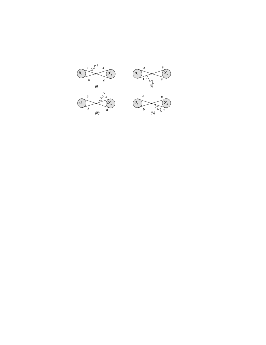
Figure 1: The weak annihilation mechanism for $B_{c}\rightarrow D_{s}^{\ast}\gamma$

The transition amplitude for this decay can be written as:

$$M(B_{c}\rightarrow D_{s}^{\ast}\gamma)=\frac{G_{F}}{\sqrt{2}}V_{cb}V_{cs}^{\ast}<D_{s}^{\ast}(p)\gamma(q)\mid(\overline{s}\Gamma_{\nu}c)(\overline{c}\Gamma^{\nu}b)\mid B_{c}(p+q)>$$ (1)

where $\Gamma_{\nu}=\gamma_{\nu}(1-\gamma_{5})$ and p, q and p+q are the momentum of $D_{s}^{\ast}$, photon and $B_{c}$, respectively. Using factorization hypothesis, The matrix element in Eq. (1) can be written in the following form:

$$<D_{s}^{\ast}(p)\gamma(q)\mid(\overline{s}\Gamma_{\nu}c)(\overline{c}\Gamma^{\nu}b)\mid B_{c}(p+q)> = -e\varepsilon^{\mu}\varepsilon^{(D_{s}^{\ast})_{\nu}}f_{D_{s}^{\ast}}m_{D_{s}^{\ast}}T_{\mu\nu}^{(B_{c})}$$ (2)

$$-ie\varepsilon^{\mu}(p+q)^{\nu}f_{B_{c}}T_{\mu\nu}^{(D_{s}^{\ast})}$$

where, the covariant decomposition of hadronic matrix elements $T_{\mu\nu}^{(B_{c})}$ and $T_{\mu\nu}^{(D_{s}^{\ast})}$ are responsible for the emission of photon from initial and final states, $f_{D_{s}^{\ast}},~{}f_{B_{c}}$ are the leptonic decay constants of $D_{s}^{\ast}$ and $B_{c}$ mesons, respectively, and $\varepsilon^{\mu}$ and $\varepsilon^{(D_{s}^{\ast})_{\nu}}$ are the polarization vectors of a photon and $D_{s}^{\ast}$ meson. The covariant decomposition of hadronic matrix elements are defined by the following two-point correlation functions:

$$T_{\mu\nu}^{(B_{c})}(p,q)=i\int d^{4}xe^{iqx}<0\mid T\{j_{\mu}^{em}\overline{c}\Gamma_{\nu}b(0)\}\mid B_{c}(p+q)>$$ (3)

and

$$T_{\mu\nu}^{(D_{s}^{\ast})}(p,q)=i\int d^{4}xe^{iqx}<D_{s}^{\ast}(p)\mid T\{j_{\mu}^{em}\overline{s}\Gamma_{\nu}c(0)\}\mid 0>$$ (4)

where $j_{\mu}^{em}$ stands for electromagnetic current. Our aim is to construct the $T_{\mu\nu}^{(B_{c})}$ and $~{}T_{\mu\nu}^{(D_{s}^{\ast})}$ in terms of form factors and other physical quantities. Let first focus on $T_{\mu\nu}^{(B_{c})}$. This quantity can be written in terms of two independent 4-momenta p and q in general as follows:

$$T_{\mu\nu}^{(B_{c})}(p,q)=g_{\mu\nu}a+p_{\mu}q_{\nu}b+q_{\mu}p_{\nu}c+p_{\mu}p_{\nu}d+q_{\mu}q_{\nu}e+\varepsilon_{\nu\mu\lambda\sigma}p^{\lambda}q^{\sigma}F_{V}^{(B_{c})}$$ (5)

where a, b, c, d, e and $F_{V}^{(B_{c})}$ are invariant amplitudes. Applying the Ward identity for electromagnetic current to Eq. (5) and using the fact that for a real photon $q^{2}=0$, we rewrite Eq.(5) in the following form:

$$T_{\mu\nu}^{(B_{c})}(p,q) = (g_{\mu\nu}(p.q)-p_{\mu}q_{\nu})iF_{A}^{(B_{c})}+g_{\mu\nu}(p.q)\alpha+p_{\mu}q_{\nu}\beta+q_{\mu}q_{\nu}c$$ (6)

$$+i\frac{p_{\mu}p_{\nu}}{p.q}f_{B_{c}}+q_{\mu}q_{\nu}e+\varepsilon_{\nu\mu\lambda\sigma}p^{\lambda}q^{\sigma}F_{V}^{(B_{c})}$$

where $F_{A}^{(B_{c})}$, $\alpha$ and $\beta$ are the new invariant amplitudes. To obtain the relation between $\alpha$ and $\beta$, we compare Eqs. (5) and (6), which leads to

$$g_{\mu\nu}a+p_{\mu}q_{\nu}b=(g_{\mu\nu}(p.q)-p_{\mu}q_{\nu})iF_{A}^{(B_{c})}+g_{\mu\nu}(p.q)\alpha+p_{\mu}q_{\nu}\beta$$ (7)

by multiplying both sides of Eq. (7) with $q^{\mu}$ and using $a+(p.q)b=if_{B_{c}}$ we get the following relation between $\alpha$ and $\beta$, which is called the Ward identity.

$$\alpha+\beta=\frac{if_{B_{c}}}{(p.q)}$$ (8)

From Eq. (8), it is clear that $\alpha$ and $\beta$ can take different choices. Within the scop of the present work, in parallel with[18], we set $\beta=0$ and $\alpha=\frac{if_{B_{c}}}{(p.q)}$. Substituting the values of $\alpha$ and $\beta$, we obtain

$$T_{\mu\nu}^{(B_{c})}(p,q) = (g_{\mu\nu}(p.q)-p_{\mu}q_{\nu})iF_{A}^{(B_{c})}+if_{B_{c}}g_{\mu\nu}+q_{\mu}q_{\nu}c$$ (9)

$$+i\frac{p_{\mu}p_{\nu}}{p.q}f_{B_{c}}+q_{\mu}q_{\nu}e+\varepsilon_{\nu\mu\lambda\sigma}p^{\lambda}q^{\sigma}F_{V}^{(B_{c})}$$

Using $\varepsilon.q=0$, $\varepsilon^{(D_{s}^{\ast})}.p=0$ and Eq. (9), we obtain the following expression for the first term in Eq. (2) in terms of two form factors ($F_{A}^{(B_{c})},~{}F_{V}^{(B_{c})}$) :

$$e\varepsilon^{\mu}\varepsilon^{(D_{s}^{\ast})_{\nu}}f_{D_{s}^{\ast}}m_{D_{s}^{\ast}}T_{\mu\nu}^{(B_{c})} = ef_{D_{s}^{\ast}}m_{D_{s}^{\ast}}\{[(\varepsilon.\varepsilon^{(D_{s}^{\ast})})(p.q)-(\varepsilon.p)(\varepsilon^{(D_{s}^{\ast})}.q)]iF_{A}^{(B_{c})}$$ (10)

$$+if_{B_{c}}(\varepsilon.\varepsilon^{(D_{s}^{\ast})})+\varepsilon_{\nu\mu\lambda\sigma}\varepsilon^{(D_{s}^{\ast})_{\nu}}\varepsilon^{\mu}p^{\lambda}q^{\sigma}F_{V}^{(B_{c})}\}$$

Omitting the details for the calculation $T_{\mu\nu}^{(D_{s}^{\ast})}$, we get the following result for the second term in the Eq. (2):

$$ie\varepsilon^{\mu}(p+q)^{\nu}f_{B_{c}}T_{\mu\nu}^{(D_{s}^{\ast})} = ief_{B_{c}}\{[(\varepsilon.\varepsilon^{(D_{s}^{\ast})})(p.q)-(\varepsilon.p)(\varepsilon^{(D_{s}^{\ast})}.q)]iF_{A}^{(D_{s}^{\ast})}$$ (11)

$$+ f_{D_{s}^{\ast}}m_{D_{s}^{\ast}}(\varepsilon.\varepsilon^{(D_{s}^{\ast})})+\varepsilon_{\nu\mu\lambda\sigma}\varepsilon^{(D_{s}^{\ast})_{\nu}}\varepsilon^{\mu}p^{\lambda}q^{\sigma}F_{V}^{(D_{s}^{\ast})}\}~{}~{}$$

where, $F_{A}^{(D_{s}^{\ast})}$ and $F_{V}^{(D_{s}^{\ast})}$ are two form factors of $D_{s}^{\ast}$. Now, we can write the transition amplitude for the radiative $B_{c}\rightarrow D_{s}^{\ast}\gamma$ decay in terms of four form factors $F_{A}^{(B_{c})}$, $F_{V}^{(B_{c})}$, $F_{A}^{(D_{s}^{\ast})}$ and $F_{V}^{(D_{s}^{\ast})}$, as follows:

$$M(B_{c}\rightarrow D_{s}^{\ast}\gamma) = e\frac{G_{F}}{\sqrt{2}}V_{cb}V_{cs}^{\ast}[-f_{D_{s}^{\ast}}m_{D_{s}^{\ast}}\{[(\varepsilon.\varepsilon^{(D_{s}^{\ast})})(p.q)-(\varepsilon.p)(\varepsilon^{(D_{s}^{\ast})}.q)]iF_{A}^{(B_{c})}$$ (12)

$$+if_{B_{c}}(\varepsilon.\varepsilon^{(D_{s}^{\ast})})+\varepsilon_{\nu\mu\lambda\sigma}\varepsilon^{(D_{s}^{\ast})_{\nu}}\varepsilon^{\mu}p^{\lambda}q^{\sigma}F_{V}^{(B_{c})}\}$$

$$-if_{B_{c}}\{[(\varepsilon.\varepsilon^{(D_{s}^{\ast})})(p.q)-(\varepsilon.p)(\varepsilon^{(D_{s}^{\ast})}.q)]iF_{A}^{(D_{s}^{\ast})}$$

$$+f_{D_{s}^{\ast}}m_{D_{s}^{\ast}}(\varepsilon.\varepsilon^{(D_{s}^{\ast})})+\varepsilon_{\nu\mu\lambda\sigma}\varepsilon^{(D_{s}^{\ast})_{\nu}}\varepsilon^{\mu}p^{\lambda}q^{\sigma}F_{V}^{(D_{s}^{\ast})}\}]$$

The form factors $F_{A}^{(B_{c})}$ and $F_{V}^{(B_{c})}$ corresponding to the emission of the photon from b and c quark (see Fig. 1 i, ii), are calculated in [2]. Therefore, we will concentrate on the calculation of the form factors $F_{A}^{(D_{s}^{\ast})}$ and $F_{V}^{(D_{s}^{\ast})}$ (see Fig.1 iii, iv).

3 Light cone QCD sum rules for the form factors $F_{A}^{(D_{s}^{\ast})}$ and $F_{V}^{(D_{s}^{\ast})}$

Based on the general idea on QCD sum rules method, we will calculate the transition form factors by equating the representation of a suitable correlator in hadronic and quark–gluon languages. For this aim, we consider the following correlation function:

$$\Pi_{\mu\nu}(p,q)=i\int d^{4}xe^{iQx}<\gamma(q)\mid T\{\overline{c}(x)\gamma_{\mu}(1-\gamma_{5})s(x)\overline{s}(0)\gamma_{\nu}c(0)\}\mid 0>$$ (13)

Here, q and p are the momentum values of photon and $D_{s}^{\ast}$, respectively and $Q=p+q$ is the transferred momentum. Now, we insert the hadronic state $D_{s}^{\ast}(p)$ to Eq. (13). This can be re-written as:

$$\Pi_{\mu\nu}(p,q)=\frac{<\gamma(q)\mid\overline{c}\gamma_{\mu}(1-\gamma_{5})s\mid D_{s}^{\ast}(p)><D_{s}^{\ast}(p)\mid\overline{s}\gamma_{\nu}c\}\mid 0>}{m_{D_{s}^{\ast}}^{2}-p^{2}}.$$ (14)

The second term in Eq. (14), by definition is:

$$<D_{s}^{\ast}(p)\mid\overline{s}\gamma_{\nu}c\mid 0>=f_{D_{s}^{\ast}}m_{D_{s}^{\ast}}\varepsilon_{\nu}^{(D_{s}^{\ast})}$$ (15)

From Fig. 1 (iii, iv) and due to the fact that parity, Lorentz and gauge invariance are musts. We can write the matrix element for the emission of the photon from $D_{s}^{\ast}$ meson as:

$$<\gamma(q)\mid\overline{c}\gamma_{\mu}(1-\gamma_{5})s\mid D_{s}^{\ast}(p)> = e\{i\varepsilon_{\mu\alpha\beta\sigma}\varepsilon^{\alpha}\varepsilon^{(D_{s}^{\ast})_{\beta}}q^{\sigma}\frac{F_{V}^{(D_{s}^{\ast})}(Q^{2})}{m_{D_{s}^{\ast}}^{2}}$$ (16)

$$+ [\varepsilon_{\mu}(\varepsilon^{(D_{s}^{\ast})}.q)-(\varepsilon.\varepsilon^{(D_{s}^{\ast})})q_{\mu}]\frac{F_{A}^{(D_{s}^{\ast})}(Q^{2})}{m_{D_{s}^{\ast}}^{2}}\}~{}~{}~{}~{}~{}$$

Substituting Eqs. (15) and (16) to (14), we have

$$\Pi_{\mu\nu}(p,q) = \frac{ef_{D_{s}^{\ast}}m_{D_{s}^{\ast}}}{m_{D_{s}^{\ast}}^{2}-p^{2}}\{i\varepsilon_{\mu\alpha\beta\sigma}\varepsilon^{\alpha}\varepsilon_{\nu}^{(D_{s}^{\ast})}\varepsilon^{(D_{s}^{\ast})_{\beta}}q^{\sigma}\frac{F_{V}^{(D_{s}^{\ast})}(Q^{2})}{m_{D_{s}^{\ast}}^{2}}$$ (17)

$$+ [\varepsilon_{\mu}\varepsilon_{\nu}^{(D_{s}^{\ast})}(\varepsilon^{(D_{s}^{\ast})}.q)-(\varepsilon.\varepsilon^{(D_{s}^{\ast})})\varepsilon_{\nu}^{(D_{s}^{\ast})}q_{\mu}]\frac{F_{A}^{(D_{s}^{\ast})}(Q^{2})}{m_{D_{s}^{\ast}}^{2}}\}$$

Summation over polarization of $D_{s}^{\ast}$ meson is performed by using:

$$\varepsilon_{\nu}^{(D_{s}^{\ast})}\varepsilon_{\beta}^{(D_{s}^{\ast})}=-g_{\nu\beta}+\frac{p_{\nu}p_{\beta}}{m_{D_{s}^{\ast}}^{2}}$$ (18)

After performing the standard calculations for the phenomenological part, we get:

$$\Pi_{\mu\nu}(p,q)=\frac{ef_{D_{s}^{\ast}}m_{D_{s}^{\ast}}}{m_{D_{s}^{\ast}}^{2}-p^{2}}\{i\varepsilon_{\mu\nu\alpha\sigma}\varepsilon^{\alpha}q^{\sigma}\frac{F_{V}^{(D_{s}^{\ast})}(Q^{2})}{m_{D_{s}^{\ast}}^{2}}+[q_{\mu}\varepsilon_{\nu}-\varepsilon_{\mu}q_{\nu}]\frac{F_{A}^{(D_{s}^{\ast})}(Q^{2})}{m_{D_{s}^{\ast}}^{2}}\}$$ (19)

The theoretical part (QCD side) of the correlator is calculated by means of OPE up to operators having dimension $d=5$ in deep Euclidean space, where both $p^{2}$ and $Q^{2}$ are large and negative. It is determined by the bare–loop (fig. 2(a, b)) and the power corrections from the operators with $d=3$, $<\overline{\psi}\psi>$, $d=4$, $m_{s}<\overline{\psi}\psi>$, $d=5$, $m_{0}^{2}<\overline{\psi}\psi>$ (fig. 2(c, d, e)) and the photon interaction with a soft quark line (fig. 2f). In calculating the bare-loop and nonperturbative correction contributions, we first write the Lorentz decomposition of the correlator as:

$$\Pi_{\mu\nu}(p,q)=i\varepsilon_{\mu\nu\alpha\sigma}\varepsilon^{\alpha}q^{\sigma}\Pi_{1}+[q_{\mu}\varepsilon_{\nu}-\varepsilon_{\mu}q_{\nu}]\Pi_{2}$$ (20)

and the dispersion representation (Cutkosky method) for the coefficients of corresponding Lorentz structures appearing in the $\Pi_{\mu\nu}(p,q)$ as follows:

$$\Pi_{1,2}(p,q)=\int ds\frac{\rho_{1,2}(s,p^{2})}{s-Q^{2}}+\mbox{subtraction terms}$$ (21)

where $\rho_{1,2}(s,p^{2})$ are spectral density corresponding to two structures in $\Pi_{\mu\nu}(p,q)$ and subtraction terms stand for corrections. To calculate $\rho_{1,2}(s,p^{2})$, we consider Feynmen diagrams in Fig. 2(a, b).

Figure 2: Feynmen diagrams for bare-loop (a, b), power corrections from the operators with 3, 4 and 5 dimensions (c, d, e) and propagation of the soft quark in electromagnetic field (f)

For instance, for the contribution of diagram (a) we get

$$T_{\mu\nu} = eN_{c}Q_{s}\int\frac{d^{4}k}{(2\pi)^{4}}$$

$$\{Tr[\frac{i(\not\!k+m_{c})}{k^{2}-m_{c}^{2}}\gamma_{\mu}(1-\gamma_{5})\frac{i(\not\!Q+\not\!k+m_{s})}{(Q+k)^{2}-m_{s}^{2}}\not\!\varepsilon\frac{i(\not\!p+\not\!k+m_{s})}{(p+k)^{2}-m_{s}^{2}}\gamma_{\nu}]\}$$

With the help of the above equations, we obtain the following expressions corresponding to the coefficients of the structures $i\varepsilon_{\mu\nu\alpha\sigma}\varepsilon^{\alpha}q^{\sigma}$ and $[q_{\mu}\varepsilon_{\nu}-\varepsilon_{\mu}q_{\nu}]$:

$$T_{1} = \frac{-eN_{c}Q_{s}}{4\pi^{2}}\{\int_{0}^{1}dxx\int_{0}^{1}dy[m_{c}m_{s}-m_{s}^{2}x\overline{y}+p^{2}(X_{1}\overline{y}+X_{3})-(p.q)(X_{2}\overline{y}^{2}$$

$$- 4x^{2}\overline{x}y+2x^{2}\overline{x}y^{2}-4x\overline{x}y)]\int_{0}^{\infty}d\alpha e^{-\alpha\Delta}\},$$

$$T_{2} = \frac{eN_{c}Q_{s}}{16\pi^{2}}\{\int_{0}^{1}dxx\int_{0}^{1}dy[m_{c}m_{s}-m_{s}^{2}x\overline{y}+p^{2}(X_{1}\overline{y}-X_{3})-(p.q)X_{3}(2\overline{y}$$ (23)

$$+ 4\overline{x}y)]\int_{0}^{\infty}d\alpha e^{-\alpha\Delta}\}$$

where $\overline{x}(\overline{y})=1-x(y)$, $\Delta=-p^{2}x\overline{x}y-Q^{2}x\overline{x}~{}\overline{y}+m_{c}^{2}\overline{x}+m_{s}^{2}x$, $X_{1}=x-2x^{2}+x^{3}$, $X_{2}=x^{2}-2x^{3}$, $X_{3}=-x+x^{2}$

In this calculation, we have also used the exponential representation for the denominator as:

$$\frac{1}{\Delta^{n}}=\frac{1}{(n-1)!}\int_{0}^{\infty}d\alpha\alpha^{n-1}e^{-\alpha\Delta}$$ (24)

Next, we apply the double Borel operator $\hat{B}(M_{1}^{2})\hat{B}(M_{2}^{2})$ on $T_{(1,2)}$ and we get:

$$\tilde{T_{1}} = \frac{-eN_{c}Q_{s}}{4\pi^{2}}\frac{\sigma_{1}\sigma_{2}}{\sigma_{1}+\sigma_{2}}\int_{0}^{1}dx\frac{1}{\overline{x}}e^{\frac{1}{x\overline{x}}(m_{c}^{2}\overline{x}+m_{s}^{2}x)(\sigma_{1}+\sigma_{2})}[m_{c}m_{s}-m_{s}^{2}x\frac{\sigma_{2}}{\sigma_{1}+\sigma_{2}}$$

$$+ p^{2}((x^{3}-2x^{2})\frac{\sigma_{2}}{\sigma_{1}+\sigma_{2}}+x^{2}-x\frac{\sigma_{1}}{\sigma_{1}+\sigma_{2}})-(p.q)(x^{2}-2x^{3}+(3x^{2}$$

$$- 4x^{3})\frac{\sigma_{1}^{2}}{(\sigma_{1}+\sigma_{2})^{2}}+(8x^{3}-2x^{2}-4x)\frac{\sigma_{1}}{\sigma_{1}+\sigma_{2}})],$$

$$\tilde{T_{2}} = \frac{eN_{c}Q_{s}}{16\pi^{2}}\frac{\sigma_{1}\sigma_{2}}{\sigma_{1}+\sigma_{2}}\int_{0}^{1}dx\frac{1}{\overline{x}}e^{\frac{1}{x\overline{x}}(m_{c}^{2}\overline{x}+m_{s}^{2}x)(\sigma_{1}+\sigma_{2})}[m_{c}m_{s}-m_{s}^{2}x\frac{\sigma_{2}}{\sigma_{1}+\sigma_{2}}$$

$$+ p^{2}((x+x^{3}-2x^{2})\frac{\sigma_{2}}{\sigma_{1}+\sigma_{2}}-x^{2}+x)-(p.q)(-2x+2x^{2})\frac{\sigma_{2}}{\sigma_{1}+\sigma_{2}}$$

$$- 2x^{3}\frac{\sigma_{2}^{2}}{(\sigma_{1}+\sigma_{2})^{2}}+(8x^{2}-4x^{3}-4x)\frac{\sigma_{1}}{\sigma_{1}+\sigma_{2}})+(2x^{3}-2x^{2})\frac{\sigma_{1}^{2}}{(\sigma_{1}+\sigma_{2})^{2}}]$$

where $\sigma_{1}=\frac{1}{M_{1}^{2}}$ and $\sigma_{2}=\frac{1}{M_{2}^{2}}$.

In deriving Eq. (3), we use the definition

$$\hat{B}(M^{2})e^{-\alpha p^{2}}=\delta(1-\alpha M^{2})$$ (26)

For the determination of the spectral density, we apply the Borel transformations to $\tilde{T_{1}}$ and $\tilde{T_{2}}$ [19] and we obtain:

$$\varrho_{1,2}(s,t,p^{2})=\frac{1}{st}\hat{B}(\frac{1}{s},\sigma_{1})\hat{B}(\frac{1}{t},\sigma_{2})\frac{\tilde{T_{1,2}}}{\sigma_{1}\sigma_{2}}$$ (27)

In this step, we use the following relations:

$$\sigma^{n}e^{-\alpha\sigma}=(-\frac{d}{d\alpha})^{n}e^{-\alpha\sigma},$$ (28)

$$\rho_{1,2}(s,p^{2})=\int dt\frac{\varrho_{1,2}(s,t,p^{2})}{t-p^{2}},$$ (29)

and

$$\hat{B}(\frac{1}{s},\sigma_{1})\hat{B}(\frac{1}{t},\sigma_{2})e^{-\alpha(\sigma_{1}+\sigma_{2})}=\delta(1-\frac{\alpha}{s})\delta(1-\frac{\alpha}{t})$$ (30)

Then, we get the following expressions for the two spectral densities, as follows:

$$\rho_{1}(s,p^{2}) = \frac{eN_{c}Q_{s}}{4\pi^{2}}\frac{1}{(s-p^{2})^{3}}\int_{x_{0}}^{x_{1}}dx\frac{1}{\overline{x}}\{(m_{c}m_{s}-m_{s}^{2}x)(s-p^{2})^{2}+p^{2}[(x^{3}-x^{2})$$

$$(s-p^{2})^{2}-x(p^{2}+\frac{m_{c}^{2}}{x}+\frac{m_{s}^{2}}{\overline{x}})(s-p^{2})]-\frac{1}{2}(m_{s}^{2}-p^{2})[(x^{2}-2x^{3})$$

$$(s-p^{2})^{2}-2(3x^{2}-4x^{3})(p^{2}+\frac{m_{c}^{2}}{x}+\frac{m_{s}^{2}}{\overline{x}})^{2}+(8x^{3}-2x^{2}-4x)(p^{2}$$

$$+\frac{m_{c}^{2}}{x}+\frac{m_{s}^{2}}{\overline{x}})(s-p^{2})]\},$$

$$\rho_{2}(s,p^{2}) = \frac{eN_{c}Q_{s}}{16\pi^{2}}\frac{1}{(s-p^{2})^{3}}\int_{x_{0}}^{x_{1}}dx\frac{1}{\overline{x}}\{[m_{c}m_{s}-m_{s}^{2}x+p^{2}(2x-3x^{2}+x^{3})]$$

$$(s-p^{2})^{2}-\frac{1}{2}(m_{s}^{2}-p^{2})[(-2x+2x^{2}-4x^{3})(s-p^{2})^{2}+(8x^{2}-4x^{3}$$

$$-4x)(p^{2}+\frac{m_{c}^{2}}{x}+\frac{m_{s}^{2}}{\overline{x}})(s-p^{2})-2(2x^{3}-2x^{2})(p^{2}+\frac{m_{c}^{2}}{x}+\frac{m_{s}^{2}}{\overline{x}})^{2}]\}$$

where the integration region is determined by the following inequality:

$$sx\overline{x}-(m_{c}^{2}\overline{x}+m_{s}^{2}x)\geq 0$$ (32)

Similar to above calculations for diagram (a), we have repeated the entire calculations for diagram (b). Finally, we get the following results for the spectral densities:

$$\rho_{1}(s,p^{2}) = \frac{eN_{c}}{48\pi^{2}}\frac{1}{(s-p^{2})^{3}}\{Q_{s}[\lambda\{3(-3+5\alpha-5\beta)p^{6}+(28+\alpha(-103$$

$$+\alpha(17+4\alpha))+52\beta-\alpha(61+8\alpha)\beta+4(10+\alpha)\beta^{2})p^{4}s-3(-2$$

$$+16\alpha^{3}+\beta-31\beta^{2}-\alpha^{2}(75+32\beta)+\alpha(39+2\beta(41+8\beta))+7\lambda^{2}$$

$$)p^{2}s^{2}+\alpha(1-86\alpha^{2}+\beta-86\beta^{2}+\alpha(67+172\beta)+18\lambda^{2})s^{3}\}+6\{$$

$$p^{6}+2m_{c}m_{s}(s-p^{2})^{2}+(2-11\alpha+4\beta)p^{4}s(-1+26\alpha^{2}+2\beta^{2}$$

$$-2\alpha(7+11\beta))p^{2}s^{2}-\alpha(1+18\alpha^{2}+2\beta(1+\beta)-4\alpha(4+5\beta))s^{3}\}$$

$$ln\frac{1+\alpha-\beta-\lambda}{1+\alpha-\beta+\lambda}]+Q_{c}[\lambda\{3(-3+5\beta-5\alpha)p^{6}+(28+\beta(-103$$

$$+\beta(17+4\beta))+52\alpha-\beta(61+8\beta)\alpha+4(10+\beta)\alpha^{2})p^{4}s-3(-2$$

$$+16\beta^{3}+\alpha-31\alpha^{2}-\beta^{2}(75+32\alpha)+\beta(39+2\alpha(41+8\alpha))+7\lambda^{2}$$

$$)p^{2}s^{2}+\beta(1-86\beta^{2}+\alpha-86\alpha^{2}+\beta(67+172\alpha)+18\lambda^{2})s^{3}\}+6\{$$

$$p^{6}+2m_{c}m_{s}(s-p^{2})^{2}+(2-11\beta+4\alpha)p^{4}s(-1+26\beta^{2}+2\alpha^{2}$$

$$-2\beta(7+11\alpha))p^{2}s^{2}-\beta(1+18\beta^{2}+2\alpha(1+\alpha)-4\beta(4+5\alpha))s^{3}\}$$

$$ln\frac{1+\beta-\tilde{\alpha}-\lambda}{1+\beta-\alpha+\lambda}]\},$$

$$\rho_{2}(s,p^{2}) = \frac{eN_{c}}{96\pi^{2}}\frac{1}{(s-p^{2})^{3}}\{Q_{s}[\lambda\{-(29+2\alpha^{2}+\beta(17+2\beta)-\alpha(19+4\beta))p^{6}$$ (33)

$$+(4\alpha^{3}+\alpha(5+\beta)(5+4\beta)-\alpha^{2}(23+8\beta)+6(8+\beta-\beta^{2}))p^{4}s$$

$$+(-23+2\alpha^{3}-5\beta(1+4\beta)+\alpha(-9+2\beta(21+\beta))+\alpha^{2}(-30$$

$$-4\beta+\frac{48}{\lambda^{2}-(1+\alpha-\beta)^{2}}))p^{2}s^{2}+\alpha(13+\alpha(-5+22\alpha)+\beta$$

$$-44\alpha\beta+22\beta^{2})s^{3}\}+6\{-2p^{6}+m_{c}m_{s}(s-p^{2})^{2}+(4+5\alpha)p^{4}s$$

$$-2(1+\alpha+4\alpha^{2}-2\alpha\beta)p^{2}s^{2}+\alpha(1+4\alpha(\alpha-\beta))s^{3}\}$$

$$ln\frac{1-\alpha+\beta-\lambda}{1-\alpha+\beta+\lambda}]+Q_{c}[\lambda\{-(29+2\beta^{2}+\alpha(17+2\alpha)-\beta(19+4\alpha))$$

$$p^{6}+(4\beta^{3}+\beta(5+\alpha)(5+4\alpha)-\beta^{2}(23+8\alpha)+6(8+\alpha-\alpha^{2}))p^{4}s$$

$$+(-23+2\beta^{3}-5\alpha(1+4\alpha)+\beta(-9+2\alpha(21+\alpha))+\beta^{2}(-30$$

$$-4\alpha+\frac{48}{\lambda^{2}-(1+\beta-\alpha)^{2}}))p^{2}s^{2}+\beta(13+\beta(-5+22\beta)+\alpha$$

$$-44\beta\alpha+22\alpha^{2})s^{3}\}+6\{-2p^{6}+m_{c}m_{s}(s-p^{2})^{2}+(4+5\beta)p^{4}s$$

$$-2(1+\beta+4\beta^{2}-2\beta\alpha)p^{2}s^{2}+\beta(1+4\beta(\beta-\alpha))s^{3}\}$$

$$ln\frac{1-\beta+\alpha-\lambda}{1-\beta+\alpha+\lambda}]\}$$

where $\alpha=\frac{m_{s}^{2}}{s}$ and $\lambda=\sqrt{1+\alpha^{2}+\beta^{2}-2\alpha-2\beta-2\alpha\beta}$.

The next step is to calculate contributions coming from the power correction terms. After standard but lengthy calculations for the contributions of the diagrams (c, d, e ), we get:

$$\Pi_{1}(p,q)^{(c,d,e)} = \frac{m_{c}}{r^{\prime}r}<\overline{s}s>-\frac{m_{s}}{2}<\overline{s}s>[\frac{m_{c}^{2}}{r^{\prime 2}r}+\frac{1}{r^{\prime}r}+\frac{m_{c}^{2}}{r^{\prime}r^{2}}]+\frac{m_{s}^{2}}{2}<\overline{s}s>[\frac{2m_{c}^{3}}{r^{\prime 3}r}$$

$$+\frac{2m_{c}^{3}}{r^{\prime 2}r^{2}}+\frac{m_{c}}{r^{\prime 2}r}+\frac{m_{c}}{r^{\prime}r^{2}}+\frac{2m_{c}^{3}}{r^{\prime}r^{3}}]-\frac{m_{0}^{2}}{4}<\overline{s}s>[\frac{2m_{c}^{3}}{r^{\prime 3}r}+\frac{2m_{c}^{3}}{r^{\prime 2}r^{2}}$$

$$+\frac{2m_{c}}{3r^{\prime 2}r}+\frac{m_{c}}{r^{\prime}r^{2}}+\frac{2m_{c}^{3}}{r^{\prime}r^{3}}],$$

$$\Pi_{2}(p,q)^{(c,d,e)} = \frac{-m_{c}}{r^{\prime}r}<\overline{s}s>+\frac{m_{s}}{2}<\overline{s}s>[\frac{m_{c}^{2}}{r^{\prime 2}r}+\frac{m_{c}^{2}}{r^{\prime}r^{2}}]-\frac{m_{s}^{2}}{2}<\overline{s}s>[\frac{2m_{c}^{3}}{r^{\prime 3}r}$$ (34)

$$+\frac{2m_{c}^{3}}{r^{\prime 2}r^{2}}+\frac{m_{c}}{r^{\prime 2}r}+\frac{m_{c}}{r^{\prime}r^{2}}+\frac{2m_{c}^{3}}{r^{\prime}r^{3}}]+\frac{m_{0}^{2}}{4}<\overline{s}s>[\frac{2m_{c}^{3}}{r^{\prime 3}r}+\frac{2m_{c}^{3}}{r^{\prime 2}r^{2}}$$

$$+\frac{2m_{c}}{3r^{\prime 2}r}+\frac{m_{c}}{r^{\prime}r^{2}}+\frac{2m_{c}^{3}}{r^{\prime}r^{3}}]$$

where $r^{2}=p^{2}-m_{c}^{2}$ and $r^{\prime 2}=Q^{2}-m_{c}^{2}$. Finally, we calculate the contribution of diagram (f). For the calculation of this diagram corresponding to the propagation of the soft quark in the external electromagnetic field, we use the light-cone expansion for the non–local operators. After contracting the c quark lines in

$$\Pi_{\mu\nu}(p,q)=i\int d^{4}xe^{iQx}<\gamma(q)\mid T\{\overline{s}(0)\gamma_{\mu}c(0)\overline{c}(x)\gamma_{\nu}(1-\gamma_{5})s(x)\}\mid 0>$$ (35)

we obtain

$$\Pi_{\mu\nu}(p,q)=i\int d^{4}x\frac{d^{4}k}{(2\pi)^{2}}\frac{e^{i(Q-k)x}}{m_{c}^{2}-k^{2}}<\gamma(q)\mid\overline{s}\gamma_{\mu}(\not\!k+m_{c})\gamma_{\nu}(1-\gamma_{5})s\}\mid 0>$$ (36)

To calculate the matrix element appearing in the above equation, we use the following identities:

$$\gamma_{\mu}\gamma_{\nu} = g_{\mu\nu}+i\sigma_{\mu\nu},$$

$$\gamma_{\mu}\gamma_{\nu}\gamma_{5} = g_{\mu\nu}\gamma_{5}-\frac{i}{2}\varepsilon_{\mu\nu\alpha\sigma}\sigma_{\alpha\sigma},$$

$$\gamma_{\mu}\gamma_{\alpha}\gamma_{\nu} = g_{\mu\alpha}\gamma_{\nu}+g_{\alpha\nu}\gamma_{\nu}-g_{\mu\nu}\gamma_{\alpha}+i\varepsilon_{\mu\nu\alpha\sigma}\gamma_{\sigma}\gamma_{5}$$ (37)

and photon distribution amplitudes (DA’s) for twist 2, 3 and 4 [20, 21]:

$$<\gamma(q)\mid\overline{s}\gamma_{\nu}s\mid 0> = -\frac{Q_{s}}{2}f_{3\gamma}\int_{0}^{1}du\overline{\psi}^{(V)}(u)x^{\theta}F_{\theta\nu}(ux)$$

$$<\gamma(q)\mid\overline{s}\gamma_{\alpha}\gamma_{5}s\mid 0> = -\frac{iQ_{s}}{4}f_{3\gamma}\int_{0}^{1}du\psi^{(A)}(u)x^{\theta}\tilde{F_{\theta\alpha}}(ux)$$

$$<\gamma(q)\mid\overline{s}\sigma_{\alpha\beta}s\mid 0> = Q_{s}<\overline{s}s>\int_{0}^{1}du\phi(u)F_{\alpha\beta}(ux)$$

$$+\frac{Q_{s}<\overline{s}s>}{16}\int_{0}^{1}dux^{2}\mathcal{A}(u)F_{\alpha\beta}(ux)$$

$$+\frac{Q_{s}<\overline{s}s>}{8}\int_{0}^{1}du\mathcal{B}(u)x^{\rho}(x_{\beta}F_{\alpha\rho}(ux)-x_{\alpha}F_{\beta\rho}(ux))$$

where $F_{\mu\nu}$ is the field strength tensor of the electromagnetic field, which is defined by

$$F_{\mu\nu}(x) = i(\varepsilon_{\nu}q_{\mu}-\varepsilon_{\mu}q_{\nu})e^{iqx}$$

$$\tilde{F_{\mu\nu}}(x) = \frac{1}{2}\varepsilon_{\mu\nu\alpha\beta}F_{\alpha\beta}(x)$$ (39)

The asymptotic expression for the photon wave function $\phi(u)$ in terms of magnetic susceptibility of the quark condensate, $\chi(\mu)$, at a re–normalization scale ($\mu=1~{}GeV^{2}$) is defined by:

$$\phi(u)=\chi(\mu)u(1-u)$$ (40)

Other functions used in Eq. (3) are defined by [20, 21]

$$\overline{\psi}^{(V)}(u) = -20u(1-u)(2u-1)+\frac{15}{16}(\omega_{\gamma}^{A}-3\omega_{\gamma}^{V})u(1-u)(2u-1)$$

$$\times(7(2u-1)^{2}-3),$$

$$\psi^{(A)}(u) = (1-(2u-1)^{2})(5(2u-1)^{2}-1)\times\frac{5}{2}(1+\frac{9}{16}\omega_{\gamma}^{V}-\frac{3}{16}\omega_{\gamma}^{A}),$$

$$\mathcal{A}(u) = 40u(1-u)(3k-k^{+}+1)+8(\xi_{2}^{+}-3\xi_{2})[u(1-u)(2+13u(1-u))$$

$$+2u^{3}(10-15u+6u^{2})lnu+2(1-u)^{3}(10-15(1-u)+6(1$$

$$-u^{2}))ln(1-u)],$$

$$\mathcal{B}(u) = 40\int_{0}^{u}d\alpha(4-\alpha)(1+3k^{+})[\frac{-1}{2}+\frac{3}{2}(2\alpha-1)^{2}]$$ (41)

where $k,~{}k^{+},~{}\xi_{2}$, $\xi_{2}^{+}$ and $f_{3\gamma}$ are constants (see [20, 21]). Using the above relations in Eq. (36), we obtain:

$$\Pi_{\mu\nu}(p,q) = -\int d^{4}x\frac{d^{4}k}{(2\pi)^{2}}\frac{e^{i(p-k)x}}{m_{c}^{2}-k^{2}}\{\frac{-Q_{s}}{2}f_{3\gamma}k_{\mu}\int_{0}^{1}du\overline{\psi}^{(V)}(u)x^{\sigma}F_{\sigma\nu}-\frac{Q_{s}}{2}f_{3\gamma}k_{\nu}$$ (42)

$$\times\int_{0}^{1}du\overline{\psi}^{(V)}(u)x^{\sigma}F_{\sigma\mu}-\frac{Q_{s}}{2}f_{3\gamma}g_{\mu\nu}k_{\alpha}\int_{0}^{1}du\overline{\psi}^{(V)}(u)x^{\sigma}F_{\sigma\alpha}+\frac{Q_{s}}{4}f_{3\gamma}$$

$$\times k_{\alpha}\int_{0}^{1}du\psi^{(A)}(u)[-x^{\alpha}F_{\mu\nu}+x_{\mu}F_{\alpha\nu}+x_{\nu}F_{\mu\alpha}]+\frac{iQ_{s}}{8}f_{3\gamma}[k_{\mu}\varepsilon_{\theta\nu\eta\lambda}$$

$$+k_{\nu}\varepsilon_{\theta\mu\eta\lambda}-g_{\mu\nu}k_{\alpha}\varepsilon_{\theta\alpha\eta\lambda}]\int_{0}^{1}du\psi^{(A)}(u)x^{\theta}F_{\eta\lambda}+\frac{iQ_{s}}{2}f_{3\gamma}k_{\alpha}\varepsilon_{\mu\nu\alpha\sigma}$$

$$\int_{0}^{1}du\overline{\psi}^{(V)}(u)x^{\theta}F_{\theta\sigma}+im_{c}[Q_{s}<\overline{s}s>\int_{0}^{1}du\phi(u)F_{\mu\nu}(ux)$$

$$+\frac{Q_{s}<\overline{s}s>}{16}\int_{0}^{1}dux^{2}\mathcal{A}(u)F_{\mu\nu}(ux)+\frac{Q_{s}<\overline{s}s>}{8}\int_{0}^{1}du\mathcal{B}(u)x^{\sigma}$$

$$\times(x_{\nu}F_{\mu\sigma}(ux)-x_{\mu}F_{\nu\sigma}(ux))]+\frac{m_{c}}{2}Q_{s}<\overline{s}s>\varepsilon_{\mu\nu\alpha\sigma}[\int_{0}^{1}du\phi(u)$$

$$\times F_{\alpha\sigma}(ux)+\frac{1}{16}\int_{0}^{1}dux^{2}\mathcal{A}(u)F_{\alpha\sigma}(ux)+\frac{1}{8}\int_{0}^{1}du\mathcal{B}(u)x^{\theta}(x_{\sigma}F_{\alpha\theta}(ux)$$

$$-x_{\alpha}F_{\sigma\theta}(ux))]\}$$

After performing integration over x and k, the following results corresponding to the coefficients of two invariant structures $i\varepsilon_{\mu\nu\alpha\sigma}\varepsilon^{\alpha}q^{\sigma}$ and $[q_{\mu}\varepsilon_{\nu}-\varepsilon_{\mu}q_{\nu}]$ are obtained as follows:

$$\Pi_{1}(p,q)^{(f)} = \frac{m_{c}Q_{s}<\overline{s}s>}{2}[\int_{0}^{1}du\phi(u)\frac{1}{p^{2}-m_{c}^{2}}-\frac{1}{16}\int_{0}^{1}du\mathcal{A}(u)(\frac{10}{(p^{2}-m_{c}^{2})^{2}}$$

$$+\frac{8m_{c}^{2}}{(p^{2}-m_{c}^{2})^{3}})],$$

$$\Pi_{2}(p,q)^{(f)} = \frac{-Q_{s}}{4}f_{3\gamma}\int_{0}^{1}du\psi^{(A)}(u)(\frac{1}{p^{2}-m_{c}^{2}}+\frac{2m_{c}^{2}}{(p^{2}-m_{c}^{2})^{2}})-m_{c}Q_{s}<\overline{s}s>$$

$$[\int_{0}^{1}du\phi(u)\frac{1}{p^{2}-m_{c}^{2}}-\frac{1}{16}\int_{0}^{1}du\mathcal{A}(u)(\frac{10}{(p^{2}-m_{c}^{2})^{2}}+\frac{8m_{c}^{2}}{(p^{2}-m_{c}^{2})^{3}})]$$

These results are the final results of the QCD part (OPE expression) of the correlator. The next step is to equate Eq. (20) and Eq. (19) (the physical or phenomenological side of the correlation function) and perform the Borel transformation, with respect to the momentum of $D_{s}^{\ast}$ meson ($p^{2}\rightarrow M_{B}^{2}$), in order to suppress the contributions of higher states and continuum. We obtain the following sum rules for the transition form factors, namely:

$$F_{V,A}^{(D_{s}^{\ast})}(Q^{2})=\frac{m_{D_{s}^{\ast}}}{f_{D_{s}^{\ast}}}e^{\frac{m_{D_{s}^{\ast}}}{M_{B}^{2}}}\hat{B}\{\int_{(m_{c}+m_{s})^{2}}^{s_{0}}ds\frac{\rho_{1,2}(s,p^{2})}{s-Q^{2}}+\Pi_{1,2}^{c+d+e+f}\}$$ (44)

where V and A are correspond to 1 and 2 in r. h. s., respectively. In Eq. (44), in order to subtract the contributions of the higher states and the continuum, quark-hadron duality assumption is used, i.e. it is assumed that

$$\rho^{higher~{}states}(s)=\rho^{OPE}(s)\theta(s-s_{0})$$ (45)

In the calculations, the following rule for the Borel transformation is used:

$$\hat{B}\frac{1}{(p^{2}-s)^{n}}=(-1)^{n}\frac{e^{\frac{-s}{M_{B}^{2}}}}{\Gamma(n)(M_{B}^{2})^{n-1}}$$ (46)

4 QCD sum rules for the form factors induced by electromagnetic penguin

The effective Hamiltonian for the $b\rightarrow s\gamma$ transition can be written as follows:

$$H=-\frac{G_{F}e}{4\pi^{2}\sqrt{2}}V_{tb}V_{ts}^{\ast}C_{7}(\mu)\overline{s}\sigma_{\mu\nu}[m_{b}\frac{1+\gamma_{5}}{2}+m_{s}\frac{1-\gamma_{5}}{2}]bF^{\mu\nu}$$ (47)

In order to obtain the transition amplitude, we need to calculate the following matrix element:

$$<D_{s}^{\ast}\mid\overline{s}\sigma_{\mu\nu}(1\pm\gamma_{5})q^{\nu}b\mid B_{c}>$$ (48)

At $q^{2}=0$, we can write this matrix element in terms of the two gauge invariant form factors $T_{1}(0)$ and $T_{2}(0)$

$$<D_{s}^{\ast}(p,\varepsilon^{(D_{s}^{\ast})})\mid\overline{s}\sigma_{\mu\nu}q^{\nu}b\mid B_{c}(Q)> = i\varepsilon_{\mu\alpha\beta\lambda}\varepsilon^{(D_{s}^{\ast})_{\alpha}}p^{\beta}Q^{\lambda}T_{1}(0),$$

$$<D_{s}^{\ast}(p,\varepsilon^{(D_{s}^{\ast})})\mid\overline{s}\sigma_{\mu\nu}q^{\nu}\gamma_{5}b\mid B_{c}(Q)> = [(m_{B_{c}}^{2}-m_{D_{s}^{\ast}}^{2})\varepsilon^{(D_{s}^{\ast})}_{\mu}$$ (49)

$$- (\varepsilon^{(D_{s}^{\ast})}.q)(p+Q)_{\mu}]T_{2}(0)$$

Using the relation

$$\sigma_{\mu\nu}\gamma_{5}=-\frac{i}{2}\varepsilon_{\mu\nu\alpha\beta}\sigma^{\alpha\beta}$$ (50)

one can immediately obtain that $T_{2}(0)$=$\frac{1}{2}T_{1}(0)$. Then, we need to calculate only the form factor $T_{1}(0)$. For this aim, we define the following three point correlation function:

$$\Pi_{\mu\alpha}=-\int d^{4}xd^{4}ye^{i(Qx-py)}<0\mid T\{\overline{c}(y)\gamma_{\alpha}s(y)\overline{s}(0)\sigma_{\mu\nu}q^{\nu}b(0)\overline{c}(x)i\gamma_{5}b(x)\}$$ (51)

where $~{}\overline{c}\gamma_{\alpha}s~{}$ and $~{}\overline{c}i\gamma_{5}b~{}$ are the interpolating currents of $D_{s}^{\ast}$ and $B_{c}$ mesons, respectively.

After inserting the hadrons full set with quantum numbers of corresponding interpolating currents (see also [12]), we obtain the following expression for the phenomenological part of the correlation function:

$$\Pi_{\mu\alpha}=i\frac{f_{B_{c}}m_{B_{c}}^{2}}{(m_{b}+m_{c})}\frac{f_{D_{s}^{\ast}}m_{D_{s}^{\ast}}}{(p^{2}-m_{D_{s}^{\ast}}^{2})(Q^{2}-m_{B_{c}}^{2})}\varepsilon_{\mu\alpha\beta\lambda}p^{\beta}Q^{\lambda}T_{1}(0)+\mbox{excited states.}$$

For the calculation of the QCD part, we write the Lorentz structure in the above correlator as:

$$\Pi_{\mu\alpha}=i\varepsilon_{\mu\alpha\beta\lambda}p^{\beta}Q^{\lambda}\Pi(p^{2},Q^{2})$$ (53)

where

$$\Pi^{per}(p^{2},Q^{2})=-\frac{1}{(2\pi)^{2}}\int d\tilde{s}ds^{\prime}\frac{\rho^{per}(p^{2},Q^{2})}{(\tilde{s}-Q^{2})(s^{\prime}-p^{2})}+\textrm{ subtraction terms}$$ (54)

The standard calculations lead to the following result for the pertubative part (bare-loop diagram):

$$\rho^{per}(s^{\prime},\tilde{s})=4N_{C}[m_{b}m_{c}(A_{1}+A_{2}+I_{0})-m^{2}_{b}A_{1}-2A_{3}]$$ (55)

where

$$A_{1} = \frac{2I_{0}}{(\tilde{s}-s^{\prime})^{2}}[s^{\prime}(\tilde{s}+m^{2}_{c}-m^{2}_{b})-\frac{1}{2}(\tilde{s}+s^{\prime})(s^{\prime}+m^{2}_{c})],$$

$$A_{2} = \frac{2I_{0}}{(\tilde{s}-s^{\prime})^{2}}[\frac{1}{2}(\tilde{s}+s^{\prime})(m^{2}_{b}-m^{2}_{c}-\tilde{s})+\tilde{s}(s^{\prime}+m^{2}_{c})],$$

$$A_{3} = I_{0}\frac{m^{2}_{b}[m^{2}_{b}s^{\prime}+(m^{2}_{c}-s^{\prime})(\tilde{s}-s^{\prime})]}{2(\tilde{s}-s^{\prime})^{2}},$$

$$I_{0} = -\frac{1}{4(\tilde{s}-s^{\prime})}$$ (56)

The integration regions over $\tilde{s}$ and $s^{\prime}$ are obtained from the following inequalities:

$$m^{2}_{c}\leq s^{\prime}\leq s^{\prime}_{0},$$

$$s^{\prime}-\frac{s^{\prime}m^{2}_{b}}{m^{2}_{c}-s^{\prime}}\leq\tilde{s}\leq\tilde{s_{0}}$$ (57)

The quark condensate terms give zero contribution after applying the double Borel transformation, with respect to the $p^{2}$ ($p^{2}\rightarrow M_{2}^{2}$) and $Q^{2}$ ($Q^{2}\rightarrow M_{1}^{2}$). Only the gluon condensates can contribute to the form factor. Fig. 3 shows such type of diagrams.

Figure 3: Feynmen diagrams for gluon corrections

After lengthy calculations for the gluon condensates contribution and equating the phenomenological and QCD parts and applying double Borel transformation with respect to the $p^{2}$ and $Q^{2}$, we find the following expression for the form factor $T_{1}(0)$:

$$T_{1}(0) = -\frac{1}{(2\pi)^{2}}\frac{(m_{b}+m_{c})}{f_{B_{c}}m_{B_{c}}^{2}f_{D_{s}^{\ast}}m_{D_{s}^{\ast}}}[\int d\tilde{s}ds^{\prime}\rho^{per}(s^{\prime},\tilde{s})e^{-\frac{\tilde{s}}{M_{1}^{2}}}e^{-\frac{s^{\prime}}{M_{2}^{2}}}$$ (58)

$$+ M_{1}^{2}M_{2}^{2}<\frac{\alpha_{s}}{\pi}G^{2}>C_{G^{2}}]$$

where $C_{G^{2}}$ is the Wilson coefficient of the gluon condensate and we thus have (see Fig. 3):

$$C_{G^{2}}=C_{G^{2}}^{a}+C_{G^{2}}^{b}+C_{G^{2}}^{c}+C_{G^{2}}^{d}+C_{G^{2}}^{e}+C_{G^{2}}^{f}$$ (59)

The explicit expressions for $C_{G^{2}}^{i}$ are given below as follows:

$$C_{G^{2}}^{a} = 96m_{b}\{[m_{c}(I_{0}[1,3,1]+m_{b}^{2}I_{0}[1,4,1]+I_{1}[1,3,1]+m_{b}^{2}I_{1}[1,4,1]$$ (60)

$$+ I_{2}[1,3,1]-m_{b}^{2}I_{2}[1,4,1])]+m_{b}(I_{1}[1,3,1]+m_{b}^{2}I_{1}[1,4,1]$$

$$+ 2I_{3}[1,4,1])\},$$

$$C_{G^{2}}^{b} = 16\{2I_{0}[1,1,2]+2m_{b}m_{c}I_{0}[1,1,3]+2I_{0}[2,1,1]+3m_{b}m_{c}I_{0}[2,1,2]$$ (61)

$$+ 4m_{c}^{2}I_{0}[2,1,2]+4m_{b}m_{c}^{3}I_{0}[2,1,3]+2m_{b}m_{c}I_{0}[3,1,1]+2m_{c}^{2}I_{0}[3,1,1]$$

$$+ 6m_{b}m_{c}^{3}I_{0}[3,1,2]+2m_{c}^{4}I_{0}[3,1,2]+2m_{b}m_{c}^{5}I_{0}[3,1,3]+2I_{1}[1,1,2]$$

$$- 2m_{b}^{2}I_{1}[1,1,3]+2m_{b}m_{c}I_{1}[1,1,3]+2I_{1}[2,1,1]-m_{b}^{2}I_{1}[2,1,2]$$

$$+ m_{b}m_{c}I_{1}[2,1,2]+4m_{c}^{2}I_{1}[2,1,2]-4m_{b}^{2}m_{c}^{2}I_{1}[2,1,3]+4m_{b}m_{c}^{3}I_{1}[2,1,3]$$

$$- 2m_{b}^{2}I_{1}[3,1,1]+2m_{c}^{2}I_{1}[3,1,1]-6m_{b}^{2}m_{c}^{2}I_{1}[3,1,2]+4m_{b}m_{c}^{3}I_{1}[3,1,2]$$

$$+ 2m_{c}^{4}I_{1}[3,1,2]-2m_{b}^{2}m_{c}^{4}I_{1}[3,1,3]+2m_{b}m_{c}^{5}I_{1}[3,1,3]+2m_{b}m_{c}I_{2}[1,1,3]$$

$$+ I_{2}[2,1,1]+m_{b}m_{c}I_{2}[2,1,2]+4m_{b}m_{c}^{3}I_{2}[2,1,3]-4m_{c}^{2}I_{2}[3,1,1]$$

$$+ 4m_{b}m_{c}^{3}I_{2}[3,1,2]+2m_{b}m_{c}^{5}I_{2}[3,1,3]-4I_{3}[1,1,3]-4I_{3}[2,1,2]$$

$$- 8m_{c}^{2}I_{3}[2,1,3]-8I_{3}[3,1,1]-16m_{c}^{2}I_{3}[3,1,2]-4m_{c}^{4}I_{3}[3,1,3]\}$$

$$- 32M_{2}^{2}\frac{d}{dM_{2}^{2}}\{M_{2}^{2}[I_{0}[2,1,2]+2m_{b}m_{c}I_{0}[2,1,3]+2m_{b}m_{c}I_{0}[3,1,2]$$

$$+ m_{c}^{2}I_{0}[3,1,2]+2m_{b}m_{c}^{3}I_{0}[3,1,3]+I_{1}[2,1,2]-2m_{b}^{2}I_{1}[2,1,3]$$

$$+ 2m_{b}m_{c}I_{1}[2,1,3]-2m_{b}^{2}I_{1}[3,1,2]+m_{b}m_{c}I_{1}[3,1,2]+m_{c}^{2}I_{1}[3,1,2]$$

$$- 2m_{b}^{2}m_{c}^{2}I_{1}[3,1,3]+2m_{b}m_{c}^{3}I_{1}[3,1,3]-I_{2}[2,1,2]+2m_{b}m_{c}I_{2}[2,1,3]$$

$$- 2I_{2}[3,1,1]+m_{b}m_{c}I_{2}[3,1,2]-m_{c}^{2}I_{2}[3,1,2]+2m_{b}m_{c}^{3}I_{2}[3,1,3]$$

$$- 4I_{3}[2,1,3]-6I_{3}[3,1,2]-4m_{c}^{2}I_{3}[3,1,3]]\}$$

$$- 32M_{2}^{4}(\frac{d^{2}}{dM_{2}^{2}})^{2}\{M_{2}^{4}[m_{b}^{2}I_{1}[3,1,3]+2I_{2}[3,1,2]-m_{b}m_{c}(I_{0}[3,1,3]$$

$$+ I_{1}[3,1,3]+I_{2}[3,1,3])+2I_{3}[3,1,3]]\}~{},$$

$$C_{G^{2}}^{c} = 96m_{c}\{-(m_{b}^{2}m_{c}I_{1}[4,1,1])+m_{b}(I_{0}[3,1,1]+m_{c}^{2}I_{0}[4,1,1]$$

$$+ I_{1}[3,1,1]+m_{c}^{2}I_{1}[4,1,1]+I_{2}[3,1,1]+m_{c}^{2}I_{2}[4,1,1])-2m_{c}I_{3}[4,1,1]\},$$

$$C_{G^{2}}^{d} = -32m_{b}m_{c}\{I_{0}[2,1,2]+I_{0}[3,1,1]+m_{c}^{2}I_{0}[3,1,2]+I_{1}[2,1,2]$$

$$+ m_{c}^{2}I_{1}[3,1,2]+I_{2}[2,1,2]+m_{c}^{2}I_{2}[3,1,2]-4I_{3}[3,1,2]$$

$$- M_{2}^{2}\frac{d}{dM^{2}}[M_{2}^{2}(I_{0}[3,1,2]+I_{1}[3,1,2]+I_{2}[3,1,2])]\}+16\{m_{b}^{2}I_{1}[2,1,2]$$

$$+ I_{2}[2,1,1]-m_{b}m_{c}(I_{0}[2,1,2]+I_{1}[2,1,2]+I_{2}[2,1,2])+4I_{3}[2,1,2]\},$$

$$C_{G^{2}}^{e} = 16\{2I_{0}[1,1,2]+I_{0}[1,2,1]+2m_{b}^{2}I_{0}[1,2,2]+m_{b}m_{c}I_{0}[1,2,2]$$ (64)

$$+ m_{c}^{2}I_{0}[2,1,2]+m_{b}m_{c}I_{0}[2,2,1]+m_{c}^{2}I_{0}[2,2,1]+m_{b}^{2}m_{c}^{2}I_{0}[2,2,2]$$

$$+ m_{b}m_{c}^{3}I_{0}[2,2,2]+I_{1}[1,1,2]+I_{1}[1,2,1]+m_{b}^{2}I_{1}[1,2,2]$$

$$+ m_{b}m_{c}I_{1}[1,2,2]-I_{1}[2,1,1]-2m_{b}m_{c}I_{1}[2,1,2]-m_{b}^{2}I_{1}[2,2,1]$$

$$+ m_{c}^{2}I_{1}[2,2,1]-2m_{b}^{3}m_{c}I_{1}[2,2,2]+m_{b}m_{c}^{3}I_{1}[2,2,2]+I_{2}[1,1,2]$$

$$+ +I_{2}[1,2,1]+m_{b}^{2}I_{2}[1,2,2]+m_{b}m_{c}I_{2}[1,2,2]-2m_{b}m_{c}I_{2}[2,2,1]$$

$$+ m_{c}^{2}I_{2}[2,2,1]+m_{b}m_{c}^{3}I_{2}[2,2,2]-2I_{3}[2,1,2]-4I_{3}[2,2,1]$$

$$- 2m_{b}^{2}I_{3}[2,2,2]-4m_{b}m_{c}I_{3}[2,2,2]\}$$

$$- 16M_{1}^{2}\frac{d}{dM_{1}^{2}}\{M_{1}^{2}[I_{2}[2,2,1]+2I_{3}[2,2,2]]\}$$

$$+ 16M_{2}^{2}\frac{d}{dM_{2}^{2}}\{M_{2}^{2}[-m_{b}m_{c}I_{0}[2,2,2]+I_{1}[2,1,2]+m_{b}^{2}I_{1}[2,2,2]$$

$$- m_{b}m_{c}I_{1}[2,2,2]+I_{2}[2,1,2]+I_{2}[2,2,1]+m_{b}^{2}I_{2}[2,2,2]$$

$$- m_{b}m_{c}I_{2}[2,2,2]+2I_{3}[2,2,2]]\}+16\{I_{1}[1,1,2]+m_{b}^{2}I_{1}[1,2,2]$$

$$+ I_{2}[1,2,1]-m_{b}m_{c}(I_{0}[1,2,2]+I_{1}[1,2,2]+I_{2}[1,2,2])$$

$$+ 2I_{3}[1,2,2]\}~{},$$

$$C_{G^{2}}^{f} = 16\{2I_{0}[1,2,1]+2I_{0}[2,1,1]+2m_{b}^{2}I_{0}[2,2,1]$$ (65)

$$+ 6m_{b}m_{c}I_{0}[2,2,1]+2m_{c}^{2}I_{0}[2,2,1]+2I_{1}[1,2,1]$$

$$- 5I_{1}[2,1,1]-5m_{c}^{2}I_{1}[2,2,1]+6m_{b}m_{c}I_{1}[2,2,1]+2m_{c}^{2}I_{1}[2,2,1]$$

$$+ 2I_{2}[1,2,1]-I_{2}[2,1,1]-m_{b}^{2}I_{2}[2,2,1]+6m_{b}m_{c}I_{2}[2,2,1]$$

$$+ 2m_{c}^{2}I_{2}[2,2,1]-14I_{3}[2,2,1]\}-32M_{1}^{2}\frac{d}{dM_{1}^{2}}\{M_{1}^{2}[I_{0}[2,2,1]$$

$$+ I_{1}[2,2,1]+I_{2}[2,2,1]]\}$$

and the for explicit form of the $I_{i}[a,b,c]$, we obtain:

$$I_{0}[a,b,c] = \frac{(-1)^{a+b+c}}{16\pi^{2}\,\Gamma(a)\Gamma(b)\Gamma(c)}(M_{1}^{2})^{2-a-b}(M_{2}^{2})^{2-a-c}\,$$

$$\times{\cal U}_{0}(a+b+c-4,1-c-b)~{},$$

$$I_{1}[a,b,c] = \frac{(-1)^{a+b+c+1}}{16\pi^{2}\,\Gamma(a)\Gamma(b)\Gamma(c)}(M_{1}^{2})^{2-a-b}(M_{2}^{2})^{3-a-c}\,$$

$$\times{\cal U}_{0}(a+b+c-5,1-c-b)~{},$$

$$I_{2}[a,b,c] = \frac{(-1)^{a+b+c+1}}{16\pi^{2}\,\Gamma(a)\Gamma(b)\Gamma(c)}(M_{1}^{2})^{3-a-b}(M_{2}^{2})^{2-a-c}\,$$

$$\times{\cal U}_{0}(a+b+c-5,1-c-b)~{},$$

$$I_{3}[a,b,c] = \frac{(-1)^{a+b+c+1}}{32\pi^{2}\,\Gamma(a)\Gamma(b)\Gamma(c)}(M_{1}^{2})^{3-a-b}(M_{2}^{2})^{3-a-c}\,$$ (66)

$$\times{\cal U}_{0}(a+b+c-6,2-c-b)$$

The function ${\cal U}_{0}(i,j)$, also, is given by:

$${\cal U}_{0}(i,j)=\int_{0}^{\infty}dy(y+M_{1}^{2}+M_{2}^{2})^{i}y^{j}\,exp\left[-\frac{B_{-1}}{y}-B_{0}-B_{1}y\right]~{},$$ (67)

where

$$B_{-1} = \frac{m_{b}^{2}}{M_{1}^{2}}\left[M_{1}^{2}+M_{2}^{2}\right]~{},$$ (68)

$$B_{0} = \frac{1}{M_{1}^{2}M_{2}^{2}}\left[M_{1}^{2}m_{c}^{2}+M_{2}^{2}(m_{c}^{2}+m_{b}^{2})\right]~{},$$ (69)

$$B_{1} = \frac{m_{c}^{2}}{M_{1}^{2}M_{2}^{2}}$$ (70)

5 Numerical analysis

In this section, we present our numerical analysis for the form factors. From the sum rule expressions of these form factors, we see that the condensates, leptonic decay constants of $B_{c}$ and $D_{s}^{\ast}$ mesons, continuum thresholds $s_{0}$, $\tilde{s_{0}}$ and $s^{\prime}_{0}$, the relevant parameters in photon distribution amplitudes (DA’s) and Borel parameters $M_{B}^{2}$, $M_{1}^{2}$ and $M_{2}^{2}$ are the main input parameters. In further numerical analysis, we choose the value of the condensates at a fixed renormalization scale of about $1$ GeV. The values of the condensates are[22]: $<\overline{\psi}\psi\mid_{\mu=1~{}GeV}>=-(240\pm 10~{}MeV)^{3}$, $<\overline{s}s>=(0.8\pm 0.2)<\overline{\psi}\psi>$ and $m_{0}^{2}=0.8~{}GeV^{2}$. The quark and mesons masses are taken to be $m_{c}(\mu=m_{c})=1.275\pm 0.015~{}GeV$, $m_{s}(1~{}GeV)\simeq 142~{}MeV$ [23] , $m_{b}=(4.7\pm 0.1)~{}GeV$ [22] , $m_{D_{s}^{\ast}}=2.112~{}GeV$ and $m_{B_{C}}=6.258~{}GeV$. For the values of the leptonic decay constants of $B_{C}$ and $D_{s}^{\ast}$ mesons, we use the results obtained from the two-point QCD analysis: $f_{B_{C}}=0.35GeV$ [26, 27, 28] and $f_{D_{s}^{\ast}}=266\pm 32~{}MeV$[24]. The relevant parameters in photon distribution amplitudes (DA’s) are taken to be $\chi=3.15\pm 0.3GeV^{-2},~{}\kappa=0.2,~{}\kappa^{+}=0,~{}\zeta_{1}=0.4,~{}\zeta_{1}^{+}=0,~{}\zeta_{2}=0.3,~{}\zeta_{2}^{+}=0,~{}f_{3\gamma}=-(4\pm 2)\times 10^{-3}GeV^{2},~{}w_{\gamma}^{A}=-2.1\pm 1.0,~{}w_{\gamma}^{V}=3.8\pm 1.8$ [20, 21, 25]. The threshold parameters are also determined from the two-point QCD sum rules: $s_{0}=8~{}GeV^{2}$ , $\tilde{s_{0}}=45~{}GeV^{2}$, $s^{\prime}_{0}=8~{}GeV^{2}$ [2, 24, 29]. The Borel parameters $M_{B}^{2}$, $M_{1}^{2}$ and $M_{2}^{2}$ are auxiliary quantities and, therefore the results of physical quantities should not depend on them. In the QCD sum rule method, OPE is truncated at finite order, leaving a residual dependence on the Borel parameters. For this reason, the working regions for the Borel parameters should be chosen such that in these regions the form factors are practically independent of them. The working regions for the Borel parameters $M_{B}^{2}$, $M_{1}^{2}$ and $M_{2}^{2}$ can be determined on the condition that, on the one side, the continuum contribution should be small, and on the other side, the contribution of the operator with the highest dimension should be small. As a result of the above-mentioned requirements, the working regions for this transition are obtained to be:

$$4~{}GeV^{2}<M_{B}^{2}<10~{}\texttt{GeV}^{2},~{}10\texttt{GeV}^{2}\leq M_{1}^{2}\leq~{}25\texttt{GeV}^{2},$$

$$4\texttt{GeV}^{2}\leq M_{2}^{2}\leq 10\texttt{GeV}^{2}.$$ (71)

Now, by calculating the total decay widths and taking $\mid V_{cs}\mid=0.957\pm 0.017$ , $\mid V_{cb}\mid=0.0416\pm 0.0006$, $\mid V_{tb}\mid=0.77^{+0.18}_{-0.24}$, $\mid V_{ts}\mid=(40.6\pm 2.7)\times 10^{-3}$ [30], $<\frac{\alpha_{s}}{\pi}G^{2}>=0.012GeV^{4}$ [29], $C_{7}(\mu=m_{c})=-0.0068-0.02i$ [13] and $\tau_{B_{c}}=0.52\times 10^{-12}s$ [31], we obtain the numerical results of the electromagnetic penguin(EP), weak annihilation(WA) and total branching ratios for this decay as follows:

$$\textbf{B}^{(EP)}(B_{c}\rightarrow D_{s}^{\ast}\gamma)=3.468\times 10^{-6}$$

$$\textbf{B}^{(WA)}(B_{c}\rightarrow D_{s}^{\ast}\gamma)=1.557\times 10^{-5}$$

$$\textbf{B}^{(Total)}(B_{c}\rightarrow D_{s}^{\ast}\gamma)=2.462\times 10^{-5}$$ (72)

From the above results, we see that the weak annihilation contribution to the total branching ratio is about $4.48$ times greater than that of the electromagnetic penguin diagram. Here, it is observed that the difference between the total branching ratio with sum of the weak annihilation and electromagnetic penguin branching ratios comes from the cross term in total decay width. Also our result for the total branching ratio shows that the $B_{c}\rightarrow D_{s}^{\ast}\gamma$ decay can be measured at LHC.

Now, we compare our results of the $B_{c}\rightarrow D_{s}^{\ast}\gamma$ to the results of the perturbative QCD [15], relativistic independent quark model [16], pertubative QCD in standard model (SM (PQCD)) [17] , multi scale walking technicolor (MWTCM) [17] and topcolor assisted MWTCM (TAMWTCM) [17] for $\tau_{B_{c}}=0.52\times 10^{-12}s$ as shown in Table (1).

	$\textbf{B}^{EP}(B_{c}\rightarrow D_{s}^{\ast}\gamma)$	$\textbf{B}^{WA}(B_{c}\rightarrow D_{s}^{\ast}\gamma)$	$\textbf{B}^{Total}(B_{c}\rightarrow D_{s}^{\ast}\gamma)$
Present study	$3.468\times 10^{-6}$	$1.557\times 10^{-5}$	$2.462\times 10^{-5}$
PQCD	$3.70\times 10^{-6}$	$4.94\times 10^{-6}$	$1.14\times 10^{-5}$
RIQM	$2.40\times 10^{-5}$	$4.51\times 10^{-5}$	$1.39\times 10^{-4}$
MWTCM	$(0.68-3.42)10^{-4}$	$(0.74-0.81)10^{-6}$	$(0.74-3.57)\times 10^{-4}$
TAMWTCM	$(5.18-7.23)10^{-7}$	$(7.24-8.13)10^{-7}$	$(1.78-9.95)\times 10^{-6}$
SM(PQCD)	$1.73\times 10^{-7}$	$5.89\times 10^{-7}$	$7.83\times 10^{-7}$

Table 1: Comparison of the branching ratio for $B_{c}\rightarrow D_{s}^{\ast}\gamma$ decay based on the $\tau_{B_{c}}=0.52\times 10^{-12}s$.

Looking at this table, it is seen that there is a good agreement between the present study and the PQCD [15], in order of magnitude for the total branching ratio. However, our result is approximately one order of magnitude less than that of the RIQM and MWTCM. Also, it is one order of magnitude and two orders of magnitude greater than that of the TAMWTCM and SM(PQCD) [17], respectively. The ratio of $\textbf{B}^{WA}/\textbf{B}^{EP}$ for the present work, PQCD [15], RIQM, SM(PQCD) [17], TAMWTCM, MWTCM are 4.48, 1.34, 1.9, 3.4, 1.23 and 0.01, respectively. As a result of the above discussions, we can say that in the QCD sum rules (present study), relativistic independent quark model, perturbative QCD and TAMWTCM approaches, the weak annihilation contribution to the total branching ratio dominates the contribution coming from the electromagnetic penguin diagram, but this is not true only for the MWTCM approach. The presence of the pseudo Goldstone bosons in the MWTCM leads to a discrepancy between this model and the other two models in [17] (for more details see[17]) and a part of inconsistency in the results of the different methods may be related to the different magnitudes of the input parameters, getting from different references; e.g. we use $m_{c}(\mu=m_{c})=1.275\pm 0.015~{}GeV$ for the c quark masses while the authors of [17] use $m_{c}=1.6~{}GeV$ and also to the nature of the methods and their accuracy.

In this step, for the analysis of $B_{c}\rightarrow D^{\ast}\gamma$, in the entire calculations we replace the s quark with the d quark. Making $m_{D_{s}^{\ast}}\rightarrow m_{D^{\ast}}$, $f_{D_{s}^{\ast}}\rightarrow f_{D^{\ast}}$, $V_{ts}\rightarrow V_{td}$, $V_{cs}\rightarrow V_{cd}$ changes and taking $m_{D^{\ast}}=2.010~{}GeV$, $f_{D^{\ast}}=0.23\pm 0.02~{}GeV$ [32], $V_{cd}=0.230\pm 0.011$, $V_{td}=(7.4\pm 0.8)\times 10^{-3}$ [30] and $m_{d}=5~{}MeV$ we obtain the numerical results as below:

$$\textbf{B}^{(EP)}(B_{c}\rightarrow D^{\ast}\gamma)=1.151\times 10^{-7}$$

$$\textbf{B}^{(WA)}(B_{c}\rightarrow D^{\ast}\gamma)=2.162\times 10^{-6}$$

$$\textbf{B}^{(Total)}(B_{c}\rightarrow D^{\ast}\gamma)=2.786\times 10^{-6}$$ (73)

These results also enhance the importance of the weak annihilation contribution to the total branching ratio in comparing with the electromagnetic penguin diagram ones for the $B_{c}\rightarrow D^{\ast}\gamma$. Finally, we compare our results to the relativistic independent quark model (RIQM) [16] for $\tau_{B_{c}}=0.52\times 10^{-12}s$ in Table (2).

	$\textbf{B}^{EP}(B_{c}\rightarrow D^{\ast}\gamma)$	$\textbf{B}^{WA}(B_{c}\rightarrow D^{\ast}\gamma)$	$\textbf{B}^{Total}(B_{c}\rightarrow D^{\ast}\gamma)$
Present study	$1.151\times 10^{-7}$	$2.162\times 10^{-6}$	$2.786\times 10^{-6}$
RIQM [16]	$5.70\times 10^{-7}$	$1.33\times 10^{-6}$	$3.64\times 10^{-6}$

Table 2: Comparison of the branching ratio for $B_{c}\rightarrow D^{\ast}\gamma$ decay based on the $\tau_{B_{c}}=0.52\times 10^{-12}s$.

From the Table 2, it is also seen a good agreement in the order of magnitude between the present study and the relativistic independent quark model.

In conclusion, the present study concentrated on the radiative $B_{c}\rightarrow D_{s}^{\ast}\gamma$ and $B_{c}\rightarrow D^{\ast}\gamma$ decays in the framework of QCD sum rules. The form factors responsible for these decays were calculated. The branching ratio for this decays were estimated. The results show that the $B_{c}\rightarrow D_{s}^{\ast}\gamma$ case can be measured at LHC in the near future.

6 Acknowledgment

One of the authors (K. Azizi) would like to thank TUBITAK, Turkish Scientific and Research Council, for their partially support. Also, V. Bashiry would like to thank theory group of CERN for their hospitality.

References

- [1] F. Abe et al. [CDF Collaboration], Phys. Rev. D 58, (1998) 112004.
- [2] T. M. Aliev, M. Savci, Phys. Lett. B 434 (1998) 358.
- [3] T. M. Aliev, M. Savci, J. Phys. G 24 (1998) 2223.
- [4] T. M. Aliev, M. Savci, Eur. Phys. J. C 47 (2006) 413.
- [5] M. A. Ivanov, J. G. Korner and P. Santorelli, Phys. Rev. D 73 (2006) 054024.
- [6] V. Bashiry, Eur. Phys. J. C 47 (2006) 423.
- [7] P. Colangelo and A. Khodjamirian, in At the Frontier of Particle Physics/Handbook of QCD, edited by M. Shifman (World Scientific, Singapore, 2001), Vol. 3, p. 1495.
- [8] P. Ball, V. M. Braun, and H. G. Dosch, Phys. Rev. D 44, (1991) 3567.
- [9] P. Ball, Phys. Rev. D 48, (1993) 3190.
- [10] A. A. Ovchinnikov and V. A. Slobodenyuk, Z. Phys. C 44, (1989) 433; V. N. Baier and A. Grozin, Z. Phys. C 47, (1990) 669 .
- [11] A. A. Ovchinnikov, Sov. J. Nucl. Phys. 50, (1989) 519 .
- [12] T. M. Aliev, K. Azizi, A. Ozpineci, Eur. Phys. J. C 51 (2007) 593.
- [13] T. M. Aliev, M. Savci, Phys. Lett. B 480 (2000) 97.
- [14] V. V. Kiselev, A. K. Likhoded, A. I. Onishchenko, Nucl. Phys. B 569 (2000) 473.
- [15] D. S. Du, X. Li, Y.Yang, Phys. Lett. B 380, (1996) 193.
- [16] N. Barik, Sk. Naimuddin, S. Kar, P. C. Dash, Phys. Rev. D 63, (2001) 014024.
- [17] Gongru Lu, Chongxing Yue, Yigang Cao, Zhaohua Xiong, Zhenjun Xiao Phys. Rev. D 54 (1996) 5647.
-
[18]
Alexander Khodjamirian, Daniel Wyler, to be published in Sergei Matinian Festschrift “From Integrable Models to Gauge Theories.”, Eds. V. Gurzadyan, A. Sedrakyan, World Scientific, 2002
arXiv: hep-ph/0111249. - [19] V. A. Nesterenko, A. V. Radyushkin, Sov. J. Nucl. Phys. 39, (1984) 811.
- [20] J. Rohrwild, Phys. Rev. D 75, (2007) 074025.
- [21] P. Ball, V. M. Braun, N. Kivel, Nucl. Phys. B 649, (2003) 263.
- [22] B. L. Ioffe, Prog. Part. Nucl. Phys. 56, (2006) 232.
- [23] Ming Qiu Huang, Phys. Rev. D69, (2004) 114015 .
- [24] P. Colangelo, F. De Fazio, and A. Ozpineci, Phys. Rev. D72, (2005) 074004.
- [25] I. I. Balitsky, V.M. Braun, and A.V. Kolesnichenko, Nucl. Phys. B 312, (1989) 509.
- [26] P. Colangelo, G. Nardulli, N. Paver, Z. Phys. C 57, (1993) 43.
- [27] V. V. Kiselev, A. V. Tkabladze, Phys. Rev. D 48, (1993) 5208.
- [28] T. M. Aliev, O. Yilmaz, Nuovo Cimento 105 A, (1992) 827.
- [29] M. A. Shifman, A. I. Vainshtein, and V. I. Zakharov, Nucl. Phys. B147, (1979) 385.
- [30] A. Ceccucci, Z. Ligeti, Y. Sakai, PDG, J. Phys. G (2006) 139.
- [31] M. Beneke, G. Buchalla, Phys. Rev. D 53, (1996) 4991.
- [32] K. C. Bowler, L. Del Debbio, J. M. Flynn, G. N. Lacagnina, V. I. Lesk, C. M. Maynard and D. G. Richards, Nucl. Phys. B 616, (2001) 507.