Dynamics of the molecular orientation field coupled to ions in two dimensional ferroelectric liquid crystals

Abstract

Molecular orientation fluctuations in ferroelectric smectic liquid crystals produce space charges, due to the divergence of the spontaneous polarization. These space charges interact with mobile ions, so that one must consider the coupled dynamics of the orientation and ionic degrees of freedom. Previous theory and light scattering experiments on thin free-standing films of ferroelectric liquid crystals have not included this coupling, possibly invalidating their quantitative conclusions. We consider the most important case of very slow ionic dynamics, compared to rapid orientational fluctuations, and focus on the use of a short electric field pulse to quench orientational fluctuations. We find that the resulting change in scattered light intensity must include a term due to the quasi-static ionic configuration, which has previously been ignored. In addition to developing the general theory, we present a simple model to demonstrate the role of this added term.

I Introduction

Quasi-elastic Rayleigh scattering is a powerful method for studying the molecular orientational fluctuations in liquid crystals orsay ; galerne . The added technique of quenching fluctuations by a short electric field pulse for ferroelectric Smectic $C^{\ast}$ (Sm $C^{\ast}$) free standing films was first applied for studying two dimensional phase transitions by Young et al. Young . By measuring the time correlation of thermal fluctuations of the $\mathbf{c}$ director orientation, they determined the ratio of the bend($K_{b}$) or splay($K_{s}$) elastic constant to the corresponding viscous coefficients($\eta_{b},\eta_{s}$) and the bend elastic constant to the square of the spontaneous polarization($P_{0}$) in the free standing film of a ferroelectric liquid crystal, that is, $K_{b}/P_{0}^{2}$, $K_{s}/\eta_{s}$, and $K_{b}/\eta_{b}$. Refining the light scattering experiment, Rosenblatt et al. Rosenblatt1 ; Rosenblatt2 performed absolute measurements of the elastic constants, spontaneous polarization, and viscosities, by monitoring the change of intensity of the scattered light due to quenching of the director fluctuations by a strong enough external electric field. As shown in Ref. Young for the director aligned along $x$ direction, the intensity of depolarized light scattered by fluctuations of wave vector $\vec{q}$ is given by

$$I(\vec{q})\propto\frac{1}{K_{s}{q_{y}}^{2}+K_{b}{q_{x}}^{2}+2\pi{P_{0}}^{2}|q_{x}|+P_{0}E},$$ (1)

where $q_{x}$ and $q_{y}$ are the components of $\vec{q}$ in a bend and a splay mode respectively, and $E$ is an external electric field. The scattering geometry was arranged such that one wave-vector mode can be probed at a time, i.e. $q_{y}=0$ for a bend mode and $q_{x}=0$ for a splay mode in Eq. (1).

However in the light scattering theory for the ferroelectric free standing liquid crystals the existence of the ionic impurities dissolved in the materials was ignored. Pindak et al. Pindak reported the ionic impurity effect on the ferroelectric free standing film qualitatively, by analyzing the change of the 2$\pi$ wall texture due to the external electric field. The relaxation time of the impurity ion fluctuations in a thin film is given by Pindak ; Rosenblattphd

$$\tau=\frac{1}{2\pi\sigma hq+Dq^{2}},$$ (2)

where $\sigma$ is conductivity, $h$ is the thickness of a film, $q$ is a wave vector, and $D$ is a diffusion constant. Using the typical values of liquid crystals, the conduction term in Eq. (2), $2\pi\sigma hq$ can be estimated as $2\times 10^{-1}$ sec^-1 and the diffusion term $Dq^{2}=9$ sec^-1. The decay rate of the fluctuations of the impurity ions is much slower than the orientation fluctuation time of the director, around 1 ms Rosenblattphd .

In a bend mode, the space charge due to divergence of the spontaneous polarization is screened on very slow time scales by impurity ions dissolved in ferroelectric liquid crystals. Similarly, slow variation in the local charge concentration due to ionic diffusion is rapidly screened by reorientation of the spontaneous polarization field, which causes reorientation of the director. In the bulk ferroelectric liquid crystals, Lu et al. Lu0 reported a very slow relaxation mode compared to a fast decay by autocorrelation measurements, which is consistent with diffusion times associated with ionic motions. In subsequent papers, they examined the coupling between the director distortions and impurity ion motions in a ferroelectric liquid crystal theoretically Lu1 and experimentally Lu2 .

In this paper, we study the dynamics of the ion-director coupling in free standing ferroelectric liquid crystal films in the 2D limit theoretically. We consider the limit of slow ion dynamics, and electric field quenching of the rapid orientation fluctuations, and find that the field induced change in light scattering intensity must include terms due to the quasi-static distribution of ions during the short applied field pulse. Without the added terms, the field quench technique produces invalid results. Additional experiments are needed to take account of this term quantitatively. They will be reported elsewhere.

This paper is organized as follows: in the next section we present the free energy of the smectic film including Frank elasticity, the coupling of the external electric field to the space charge, the energy associated with fluctuations in the ionic impurity concentration, and the electrostatic energy of the space and ionic charges. In Sec. III we analyze the relaxational dynamics of the coupled director and ionic degrees of freedom, and provide physical insight into the central result of this analysis using a simple spring–based model. Concluding remarks including comments on the experimental implications of our work are offered in the final section.

II Free Energy

In the Sm $C^{\ast}$ phase, there exist both tilt angle and azimuthal fluctuations blinc ; degenne . Here we consider temperatures sufficiently below the Sm$C^{\ast}-A$ transition so that the tilt angle fluctuations are small and we need only study fluctuations in the azimuthal angle $\varphi$. Therefore, the magnitude of $\mathbf{c}$ director is constant in the film and the molecules fluctuate azimuthally about $<\varphi_{0}>$, which is the average azimuthal orientation (see Fig. 1).

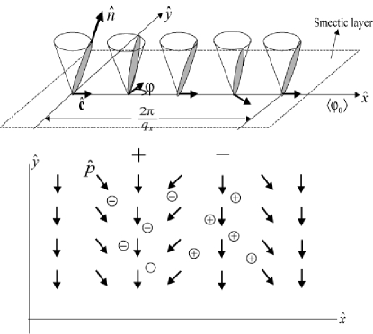
Figure 1: Top: Bend mode of the $\mathbf{c}$ director. Bottom: The transverse dipole $\mathbf{p}$ alignment accompanying the bend mode of the $\mathbf{c}$ director. The arrows denote the direction of the local dipole moment which is perpendicular to the $\mathbf{c}$ director. The impurity ions dissolved in the material are coupled to the space charge (indicated by the pluses and minuses) Rosenblattphd .

We assume that the liquid crystal film lies in the plane $z=0$, surrounded by vacuum on both sides. Average alignment of the molecules is achieved by an external electric field small enough so as not to suppress the thermal fluctuations. In a bend mode of the $\mathbf{c}$ director, the divergence of the transverse dipoles gives rise to space charge. The variation of the space charge due to the azimuthal fluctuations causes diffusion of the free ions dissolved in the film. Hence the ionic diffusion is observable in a light scattering experiment. When the molecular orientation fluctuates by an angle $\varphi$ from $<\varphi_{0}>=0$, the $\mathbf{c}$ director can be expressed by

$$\mathbf{c}=(\cos{\varphi(x,y)},\sin{\varphi(x,y)}).$$ (3)

The Frank elastic free energy density of a two–dimensional (2D) Sm $C$ is given by Young ,

$$f_{el}=\frac{1}{2}K_{s}(\nabla\cdot\mathbf{c})^{2}+\frac{1}{2}K_{b}(\nabla\times\mathbf{c})^{2},$$

which for small fluctuations can be approximated by,

$$f_{el}={\frac{1}{2}{K_{s}\Big{(}\frac{\partial\varphi}{\partial y}\Big{)}^{2}+\frac{1}{2}K_{b}(\frac{\partial\varphi}{\partial x})^{2}}},$$ (4)

The splay and bend Frank elastic constants are denoted by $K_{s}$ and $K_{b}$, respectively. The Fourier transform of $f_{el}$ is given by

$$f_{el}(\mathbf{q}_{\perp})=\frac{1}{2}K_{s}q_{y}^{2}|\varphi(\mathbf{q}_{\perp})|^{2}+\frac{1}{2}K_{b}q_{x}^{2}|\varphi(\mathbf{q}_{\perp})|^{2}.$$ (5)

where

$$\varphi(\mathbf{q}_{\perp})=\int{\varphi(\mathbf{r}_{\perp})\exp{(i\mathbf{q}_{\perp}\cdot\mathbf{r}_{\perp})}}\frac{d^{2}{r}_{\perp}}{(2\pi)^{2}},$$ (6)

Here we denote the 2D position vector and wavevector by $\mathbf{r}_{\perp}=(x,y)$ and $\mathbf{q}_{\perp}=(q_{x},q_{y})$ respectively.

The total electrostatic free energy includes the interaction energy $F_{P}$ of the polarization $\mathbf{P}$ with the external electric field $\mathbf{E}$ and the electrostatic energy $F_{E}$ of the space and impurity charges. The Fourier transform of the free energy density $f_{P}$ associated with $F_{P}$ is given by Young :

$$f_{P}({\mathbf{q}_{\perp}})=\frac{1}{2}P_{0}E|\varphi(\mathbf{q}_{\perp})|^{2},$$ (7)

where we have again assumed small azimuthal fluctuations and neglected the energy associated with the equilibrium configuration. Note that this energy density is identical for bend and splay modes.

If we consider $n$ kinds of impurity ions, such that the equilibrium concentration of the $i^{th}$ type of impurity is $c_{i}$ and the local concentration fluctuation is $\delta c_{i}$, then the free energy density $f_{ion}$ associated with fluctuations of the impurity ions is given by Lu1 :

$$f_{ion}(\mathbf{r}_{\perp})=\frac{1}{2}k_{B}T\sum^{n}_{i=1}{\frac{(\delta c_{i}(\mathbf{r}_{\perp}))^{2}}{c_{i}}},$$ (8)

where $k_{B}$ is the Boltzmann constant and $T$ is the temperature. The Fourier transform of this last equation is

$$f_{ion}(\mathbf{q}_{\perp})=\frac{1}{2}k_{B}T\sum^{n}_{i=1}{\frac{(\delta c_{i}(\mathbf{q}_{\perp}))^{2}}{c_{i}}}.$$ (9)

The total charge density $\rho(\mathbf{r})$ for an infinitesimally thin film is given by

$$\rho(\mathbf{r})=\sigma(\mathbf{r}_{\perp})\delta(z)=[\sigma_{ion}(\mathbf{r}_{\perp})+\sigma_{P}(\mathbf{r}_{\perp})]\delta(z),$$ (10)

where $\sigma_{P}(\mathbf{r}_{\perp})=-\nabla\cdot\mathbf{P}$ is the space charge density due to the divergence of the spontaneous polarization and the ionic charge density $\sigma_{ion}$ is given by

$$\sigma_{ion}(\mathbf{r}_{\perp})=\sum_{i=1}^{n}e_{i}\delta c_{i}(\mathbf{r}_{\perp}),$$ (11)

where $e_{i}$ is the charge of ionic species $i$. Here $\mathbf{r}$ is the full 3D position vector $\mathbf{r}=(x,y,z)$.

The electrostatic free energy of the film (excluding the interaction with the external electric field) is given by:

$$F_{e}=\frac{1}{2}\int{\rho(\bm{r})\Phi(\bm{r})d^{3}{r}},$$ (12)

where $\Phi$ is the electrostatic potential of the charge density $\rho$ in a dielectric medium with dielectric constant:

$$\varepsilon^{\prime}(z)=1+(\varepsilon-1)a\delta(z).$$ (13)

Here we assume that the liquid crystal film has uniform dielectric constant $\varepsilon$ and is surrounded by vacuum on both sides. Mathematically we treat the film as infinitesimally thin, but introduce the film thickness $a$ in an appropriate dimensional fashion.

As shown in Ref. lee:051701 the electrostatic free energy can be expressed in Fourier space by

$$F_{e}=\int f_{e}(\mathbf{q}_{\perp}){d^{2}q_{\perp}\over(2\pi)^{2}},$$ (14)

where the free energy density $f_{e}(\mathbf{q}_{\perp})$ is given by:

$$f_{e}(\mathbf{q}_{\perp})=\sigma(\mathbf{q}_{\perp})\sigma(-\mathbf{q}_{\perp}){2\pi\over 2q_{\perp}+(\varepsilon-1)aq_{\perp}^{2}},$$ (15)

which in the long–wavelength limit of experimental relevance ($q_{\perp}a\ll 1$) simplifies to:

$$f_{e}(\mathbf{q}_{\perp})\approx\sigma(\mathbf{q}_{\perp})\sigma(-\mathbf{q}_{\perp}){\pi\over q_{\perp}}.$$ (16)

The spontaneous polarization $\mathbf{P}$ is given by $\mathbf{P}=P_{0}[\sin{\varphi}\mathbf{\hat{x}}-\cos{\varphi}\mathbf{\hat{y}}]$ in the geometry of Fig. 1. The space charge density $\sigma_{P}$ is given for small fluctuations by

$$\sigma_{P}(x)\approx-P_{0}\frac{\partial\varphi}{\partial x},$$ (17)

with Fourier transform:

$$\sigma_{P}(\mathbf{q}_{\perp})\approx iP_{0}\varphi(\mathbf{q}_{\perp})q_{x}.$$ (18)

We note that only bend mode fluctuations contribute to the space charge, and we henceforth consider $\mathbf{q}_{\perp}=(q,0)$. The total Fourier–transformed charge density is given by

$$\sigma{(q)}=iP_{0}\varphi(q)q+\sum_{i=1}^{n}e_{i}\delta c_{i}(\mathbf{q}).$$ (19)

Substituting Eq. (19) into Eq. (16), we obtain

$$f_{e}(q) = \frac{\pi}{q}\Big{[}iP_{0}\varphi(q)q+\sum_{i=1}^{n}e_{i}\delta c_{i}(q)\Big{]}\Big{[}-iP_{0}\varphi^{*}(q)q+\sum_{j=1}^{n}e_{j}\delta c_{j}^{*}(q)\Big{]}$$ (20)

$$f_{e}(q) = \pi P_{0}^{2}q|\varphi(q)|^{2}+\sum_{i=1}^{n}\frac{\pi}{q}e_{i}^{2}|\delta c_{i}(q)|^{2}+\frac{\pi}{2q}\sum_{i\not=j}e_{i}e_{j}\delta c_{i}(q)\delta c^{\ast}_{j}(q)$$ (21)

$$+i\pi P_{0}\sum_{i=1}^{n}e_{i}(\varphi(q)\delta c_{i}^{\ast}(q)-\varphi^{\ast}(q)\delta c_{i}(q)),$$

Using Eqs. (5), (7), (9), and (20) the Fourier transformed free energy density is then given by:

$$f(q) = f_{el}(q)+f_{P}(q)+f_{ion}(q)+f_{e}(q)$$ (23)

$$= \biggl{(}{1\over 2}K_{b}q^{2}+{1\over 2}P_{o}E+\pi P_{0}^{2}q\biggr{)}|\varphi(q)|^{2}+\sum_{i=1}^{n}\biggl{(}\frac{\pi}{q}e_{i}^{2}+\frac{1}{2}\frac{k_{B}T}{c_{i}}\biggr{)}|\delta c_{i}(q)|^{2}$$

$$+i\pi P_{0}\sum_{i=1}^{n}e_{i}(\varphi(q)\delta c_{i}^{\ast}(q)-\varphi^{\ast}(q)\delta c_{i}(q))$$

$$+\frac{\pi}{2q}\sum_{i\not=j}e_{i}e_{j}\delta c_{i}(q)\delta c^{\ast}_{j}(q),$$

III Dynamics

We now consider the dynamics of the director and ionic fluctuations following the approach of Ref. Lu1 where a bulk system was considered. We model the dynamics of the film with a relaxational equation, assuming a viscosity $\eta$ associated with bend fluctuations:

$$\eta\frac{\partial\varphi(q,t)}{\partial t} = -\frac{\partial f(q,t)}{\partial\varphi_{-q,t}}+g(t)$$

$$= -(K_{b}q^{2}+P_{0}E+2\pi P_{0}^{2}q)\varphi(q,t)+2\pi iP_{0}\sum_{i=1}^{n}e_{i}\delta c_{i}(q,t)+g(t),$$

where $g(t)$ is a random noise source with zero mean and autocorrelation function given by:

$$<g(t)g(t^{\prime})>=2k_{B}T\eta\delta(t-t^{\prime}).$$ (25)

The dynamical equation for the concentration fluctuations is governed by charge conservation, which in Fourier space reads:

$$\frac{\partial\delta c_{i}(q,t)}{\partial t}=-iqJ_{i}(q,t),\ \ i=1,...,n,$$ (26)

where the current $J_{i}$ is given by $J_{i}(q,t)=-iqm_{i}c_{i}[\partial f(q,t)/\partial\delta c_{i}(-q,t)]$, and $m_{i}$ is the mobility of the ion of type i. Thus, Eq. (26) can be written as:

$$\frac{\partial\delta c_{i}(q,t)}{\partial t} = -m_{i}c_{i}q^{2}\frac{\partial f(q,t)}{\partial\delta c_{i}(-q,t)},\ \ i=1,...,n,$$ (27)

$$= -m_{i}k_{B}Tq^{2}\delta c_{i}(q,t)-2\pi m_{i}c_{i}e_{i}q\sigma(q,t),\ \ i=1,...,n,$$ (28)

where we have used Eq. (19).

We solve Eqs. (LABEL:phieqn) and (28) by Laplace transforming in time. To simplify the calculation we assume that the ionic mobility $m_{i}$ is independent of the ion type i; we denote this common value by m. We introduce the Laplace transforms of $\varphi,\delta c_{i},g(s)$, and $\sigma$ as follows:

$$\varphi(q,s) = \int^{\infty}_{0}dte^{-st}\varphi(q,t)$$ (29)

$$\delta c(q,s) = \int^{\infty}_{0}dte^{-st}\delta c(q,t)$$ (30)

$$\sigma(q,s) = \int^{\infty}_{0}dte^{-st}\sigma(q,t)$$ (31)

$$g(s) = \int^{\infty}_{0}dte^{-st}g(t)$$ (32)

Using Eqs. (29)–(32), we Laplace transform Eqs. (LABEL:phieqn) and (28) and find:

$$\eta(s\varphi(q,s)-\varphi_{o}(q)) = -(K_{b}q^{2}+P_{0}E+2\pi P_{0}^{2}q)\varphi(q,s)$$ (33)

$$+2\pi iP_{0}\sum_{i=1}^{n}e_{i}\delta c_{i}(q,s)+g(s)$$

$$s\delta c_{i}(q,s)-\delta c_{io}(q) = -m_{i}k_{B}Tq^{2}\delta c_{i}(q,s)-2\pi m_{i}c_{i}e_{i}q\sigma(q,s),$$ (34)

$$i=1,...,n,$$

where, $\varphi_{o}(q)\equiv\varphi(q,t=0)$, and $\delta c_{io}(q)\equiv\delta c_{i}(q,t=0)$.

We eliminate $\delta c_{i}(q,s)$ from Eq. (33) using the definition of $\sigma(q,s)$, Eq. (19):

$$\eta(s\varphi(q,s)-\varphi_{o}(q))=-(K_{b}q^{2}+P_{0}E)\varphi(q,s)+2\pi iP_{0}\sigma(q,s)+g(s),$$ (35)

and eliminate $\delta c_{i}(q,s)$ from Eq. (34) by first multiplying the latter equation by $e_{i}$ and then summing over i. Using Eq. (19) we obtain:

$$(s+mk_{B}Tq^{2})(\sigma(q,s)-iP_{0}q\varphi(q,s))=\sigma_{o}(q)-iP_{0}\varphi_{o}(q)-2\pi mq\sigma(q,s)\sum_{i=1}^{n}e^{2}_{i}c_{i},$$ (36)

where $\sigma_{o}(q)\equiv\sigma(q,t=0)$.

Finally, eliminating $\sigma(q,s)$ from Eqs. (35) and (36) we obtain the following solution for $\varphi(q,s)$:

$$\varphi(q,s)={g(s)+\eta\varphi_{o}(q)+2\pi iP_{0}{\sigma_{o}(q)-iP_{0}q\varphi_{o}(q)\over s+mk_{B}Tq^{2}+2\pi mq\sum_{i}e^{2}_{i}c_{i}}\over\eta s+K_{b}q^{2}+P_{0}E+{2\pi P_{0}^{2}\over\frac{2\pi m}{s+mk_{B}Tq^{2}}\sum_{i}e^{2}_{i}c_{i}+\frac{1}{q}}}$$ (37)

This expression for $\varphi(q,s)$ is of the form:

$$\varphi(q,s)=A(s)g(s)+B(s),$$ (38)

where:

$$A(s) = 1\over\eta s+K_{b}q^{2}+P_{0}E+{2\pi P_{0}^{2}\over\frac{2\pi m}{s+mk_{B}Tq^{2}}\sum_{i}e^{2}_{i}c_{i}+\frac{1}{q}}$$ (39)

$$B(s) = {\eta\varphi_{o}(q)+2\pi iP_{0}{\sigma_{o}(q)-iP_{0}q\varphi_{o}(q)\over s+mk_{B}Tq^{2}+2\pi mq\sum_{i}e^{2}_{i}c_{i}}\over\eta s+K_{b}q^{2}+P_{0}E+{2\pi P_{0}^{2}\over\frac{2\pi m}{s+mk_{B}Tq^{2}}\sum_{i}e^{2}_{i}c_{i}+\frac{1}{q}}}.$$ (40)

The convolution theorem for Laplace transforms then yields the following solution for $\varphi$ as a function of time:

$$\varphi(q,t)={\cal L}^{-1}[B(s)]+\int^{t}_{o}A(t-t^{\prime})g(t^{\prime})dt^{\prime},$$ (41)

where the operator ${\cal L}^{-1}$ is the inverse Laplace transform, and $A(t)={\cal L}^{-1}[A(s)]$.

We evaluate the inverse Laplace transforms appearing in Eq. (41) using the Bromwich integral:

$${\cal L}^{-1}[A(s)]=\sum\mbox{residues of the poles of}\ A(s)e^{st}.$$ (42)

The functions $A(s)$ and $B(s)$ have identical simple poles at $s=s_{1},s_{2}$:

$$s_{1,2}={-\alpha\pm\sqrt{\alpha^{2}-4\eta\beta}\over 2\eta},$$ (43)

where

$$\alpha = 2\pi P_{0}^{2}q+K_{b}q^{2}+P_{0}E+2\pi\eta mq\sum_{i}e_{i}^{2}c_{i}+\eta mk_{B}Tq^{2},$$ (44)

$$\beta = (K_{b}q^{2}+P_{0}E)(mk_{B}Tq^{2}+2\pi mq\sum_{i}e_{i}^{2}c_{i})+2\pi P_{0}^{2}mk_{B}Tq^{3}$$ (45)

It is instructive to examine some limiting cases of these poles as was done in Ref. Lu1 .

Static ions: $m=0$.

In this case the locations of the poles are given by:

$$s_{1}=-\eta^{-1}(K_{b}q^{2}+P_{0}E+2\pi P_{0}^{2}q),\ \ s_{2}=0,$$ (46)

i.e., $s_{1}$ describes the director relaxation rate in the absence of ions, while $s_{2}$ corresponds to the infinite relaxation time of the static ions.

Static director: $K_{b}=P_{0}=0$.

Here the poles are given by:

$$s_{1}=0,\ \ s_{2}=2\pi mq\sum_{i}e^{2}_{i}c_{i}+mk_{B}Tq^{2},$$ (47)

where $s_{2}$ is the relaxation rate of the ions, and $s_{1}$ describes the static director. These results agree with the corresponding results found in Ref. Lu1 for the bulk ferroelectric liquid crystal.

Returning to Eq. (41), we evaluate $<|\varphi(q,t)|^{2}>$, a quantity proportional to the scattered light intensity. The brackets refer to an average over the Boltzmann ensemble of $\phi_{o}$ and $\sigma_{o}$ (which appear in $B(s)$), and the random noise source $g(t)$, whose variance is given by Eq. (25). We find:

$$<|\varphi(q,t)|^{2}>=<|B(q,t)|^{2}>+2\eta k_{B}T\int^{t}_{o}A^{2}(t-t^{\prime})dt^{\prime}.$$ (48)

While the averages and integral in Eq. (48) can in principle be evaluated for arbitrary values of the ionic mobility, bend elastic constant and polarization, the expressions obtained are rather complicated, so we consider instead the experimentally relevant case where the ionic mobility $m\rightarrow 0$ and assume that the electric field is switched on at $t=0^{+}$. Using Eqs. (19), (37), (42) and (46), we find from Eq. (48):

$$\lim_{t\to\infty}<|\varphi(q,t)|^{2}> = {(2\pi P_{0})^{2}\over(K_{b}q^{2}+P_{0}E+2\pi P_{0}^{2}q)^{2}}<|\sum_{i}e_{i}\delta c_{i}|^{2}>_{o}$$ (49)

$$+{k_{B}T\over K_{b}q^{2}+P_{0}E+2\pi P_{0}^{2}q},$$

where the thermal average is over the Boltzmann ensemble at $t=0$ when $E=0$. Using Eq. (23) we find:

$$<|\sum_{i}e_{i}\delta c_{i}|^{2}>_{o}=k_{B}T{K_{b}q+2\pi P_{0}^{2}\over 4\pi\lambda_{2D}(K_{b}q+2\pi P_{0}^{2})+2\pi K_{b}}$$ (50)

where $\lambda_{2D}$ is the Debye screening length in 2D defined by

$$\lambda_{2D}\equiv\frac{k_{B}T}{4\pi\sum_{i}c_{i}e_{i}^{2}}.$$ (51)

The expression Eq. (49) for $<|\varphi(q,t)|^{2}>$ can be given a simple physical interpretation. In the limit of static ions where $m=0$, the director angle $\varphi$ has a mean value given by:

$$<\varphi(q,t)>=<B(t)>={2\pi iP_{0}\sum_{i}e_{i}\delta c_{i}\over K_{b}q^{2}+P_{0}E+2\pi P_{0}^{2}q}$$ (52)

using Eqs. (40) and (41), and recalling that the noise source $g(t)$ has zero mean. More simply, this result can be obtained by averaging Eq. (LABEL:phieqn) over the noise and noting that $<{\partial\varphi(q,t)\over\partial t}>=0$.

We now write $\varphi$ as:

$$\varphi(q,t)=<\varphi(q,t)>+(\varphi(q,t)-<\varphi(q,t)>),$$ (53)

and note that the fluctuation of $\varphi$ about its mean value, Eq. (52), has a mean-squared average:

$$<|\varphi(q,t)-<\varphi(q,t)>|^{2}>={k_{B}T\over K_{b}q^{2}+P_{0}E+2\pi P_{0}^{2}q},$$ (54)

as can be seen using Eq. (23).

Then, it can be readily seen that the mean–squared average of $\varphi$,

$$<|\varphi(q,t)|^{2}>=|<\varphi(q,t)>|^{2}+<|\varphi(q,t)-<\varphi(q,t)>|^{2}>,$$ (55)

yields Eq. (49) in the long–time limit. Note that because the ions are static, the application of the electric field at $t=0$ has no effect on the value of $<|\sum_{i}e_{i}\delta c_{i}|^{2}>_{o}$ which enters the first term on the right–hand side of Eq. (55).

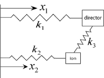
Figure 2: A toy model for the coupling between director and ionic degrees of freedom.

Additional physical insight into Eq. (49) can be obtained by considering the toy model shown in Fig. 2. We represent the director mode by a single variable $x_{1}$ and the ionic displacement mode by the single variable $x_{2}$. The spring constants $k_{1}$ and $k_{2}$ represent the corresponding restoring forces for these modes. A third spring constant $k_{3}$ represents the coupling of the director and ion fluctuations. The energy of director fluctuations in this model in the absence of an external electric field is given by,

$$F = \frac{1}{2}k_{1}x_{1}^{2}+\frac{1}{2}k_{3}(x_{2}-x_{1})^{2}$$ (56)

$$= \frac{1}{2}(k_{1}+k_{3})x_{1}^{2}-k_{3}x_{1}x_{2}+\frac{1}{2}k_{3}x_{2}^{2}.$$

The equilibrium value of $x_{1}$ which we denote by $\bar{x}_{1}$ is given by solving $\partial F/\partial x_{1}=0$ with the result:

$$\bar{x}_{1}=\frac{k_{3}}{k_{1}+k_{3}}x_{2}.$$ (57)

Defining the variation $y=x_{1}-\bar{x}_{1}$ of $x_{1}$ about its equilibrium position $\bar{x_{1}}$, the spring free energy in Eq. (56) can be rewritten as

$$F=\frac{1}{2}(k_{1}+k_{3})y^{2}+\textrm{constant}.$$ (58)

Using the equipartition theorem the thermal average of the square of $y$ is given by

$$<y^{2}>=\frac{k_{B}T}{k_{1}+k_{3}}.$$ (59)

and the corresponding quantity for $x_{1}$ is given by

$$<x_{1}^{2}> = <\bar{x}_{1}^{2}+y>$$ (60)

$$= <\bar{x}_{1}^{2}>+2<\bar{x}_{1}y>+<y^{2}>$$

$$= \frac{k_{3}^{2}}{(k_{1}+k_{3})^{2}}<x_{2}^{2}>+\frac{k_{B}T}{k_{1}+k_{3}},$$ (61)

where $<\bar{x}_{1}y>=0$ because $x_{1}$ and $y$ are statistically independent in our model. This equation is analogous to Eq. (55) above. Now, imagine a sudden application of the external electric field $E$ which leads to the replacement of the spring constant $k_{1}$ by $k_{1}+E$. If we assume that the free ions have a very long decay time then $x_{2}$ can be considered a constant during the electric field pulse. Hence with the application of the electric field, $<x_{1}^{2}>$ is given by

$$<x_{1}^{2}(E\neq 0)>=\frac{k_{3}^{2}}{(k_{1}+E+k_{3})^{2}}<x_{2}^{2}>+\frac{k_{B}T}{k_{1}+E+k_{3}}.$$ (62)

This expression is analogous to our central result Eq. (49) above. The second term on the right–hand side of Eq. (62) corresponds to $<y^{2}>$, the fluctuation of $x_{1}$, the director mode, about its mean value $\bar{x}_{1}$, while the first term corresponds to $<\bar{x}_{1}^{2}>$, which in turn depends on the ionic degree of freedom $x_{2}$, as indicated in Eq. (57).

IV Conclusions

In this paper we have considered the coupled dynamics of the orientational and ionic degrees of freedom in thin freely–suspended smectic liquid crystal films. Our central result shown in Eqs. (49)–(50) describes the fluctuations in the azimuthal angle of the $\mathbf{c}$ director, which is proportional to the scattered light intensity. As illustrated in our toy model at the end of the last section, the fluctuations can be understood as arising from two contributions: the director fluctuations measured relative to their mean value (the second term on the right–hand sides of Eqs. (49) and (62)) and the change in this mean value due to coupling to the ions (the first term on the right–hand side of Eqs. (49) and (62)). Previous theoretical and experimental work on smectic films which ignored the existence of ionic impurities thus ignored the second contribution to the light scattering intensity. While we have shown that in principle the ionic impurities will modify the light scattering intensity the effect might in practice be negligible. Upon using Eq. (50) the ionic contribution to the director fluctuations (the first term on the right–hand side of Eq. (49)) is given by:

$$\frac{(2\pi P_{0})^{2}}{(K_{b}q^{2}+P_{0}E+2\pi P_{0}^{2}q)^{2}}\bigg{[}\frac{k_{B}T(K_{b}q+2\pi P_{0}^{2})}{4\pi\lambda_{2D}(K_{b}q+2\pi P_{0}^{2})+2\pi K_{b}}\bigg{]}.$$ (63)

If the screening length $\lambda_{2D}$ is shorter than a few microns at wavevectors in the range $2000\sim 5000cm^{-1}$, the ionic contribution is not small compared to the second term in Eq. (49). However, if $\lambda_{2D}\gtrsim 10\mu$m, then the ionic contribution, Eq. (63), contributes less than 10$\%$ to the expression Eq. (49) for the director fluctuations. Therefore for any particular experiment one must evaluate the relative importance of the ionic contribution shown in Eq. (63).

References

• (1) Orsay liquid crystal group, Phys. Rev. Lett. 22, 1361 (1969)
• (2) Y. Galerne, J. L. Martinand, G. Durand, and M. Veyssie, Phys. Rev. Lett. 29, 562 (1972)
• (3) C. Y. Young, R. Pindak, N. A. Clark, and R. B. Meyer, Phys. Rev. Lett. 40, 773 (1978)
• (4) C. Rosenblatt, R. Pindak, N. A. Clark, and R. B. Meyer, Phys. Rev. Lett. 42, 1220 (1979)
• (5) C. Rosenblatt, R. B. Meyer, R. Pindak, and N. A. Clark, Phys. Rev. A 21, 140 (1980)
• (6) R. Pindak, C. Y. Young, R. B. Meyer, and N. A. Clark, Phys. Rev. Lett. 45, 1193 (1980)
• (7) C. Rosenblatt, Ph.D. Thesis, Harvard University, (1978)
• (8) M. H. Lu, K. A. Crandall, and C. Rosenblatt, Phys. Rev. Lett. 68, 3575 (1992)
• (9) M. H. Lu, C. Rosenblatt, and R. G. Petschek, Phys. Rev. E 47, 1139 (1993)
• (10) M. H. Lu, C. Rosenblatt, Phys. Rev. E 48, R2370 (1993)
• (11) R. Blinc and B. Zeks, Phys. Rev. A 18, 740 (1978)
• (12) P. G. de Gennes and J. Prost, The Physics of Liquid Crystals, 2nd ed. (Clarendon Press, Oxford, 1995)
• (13) J.–B. Lee, R. A. Pelcovits and R. B. Meyer, Phys. Rev. E 75, 051701 (2007).