Doppler shift oscillations in solar spicules

Abstract

Context. Consecutive height series of H${\alpha}$ spectra in solar limb spicules taken on the 53 cm coronagraph of Abastumani Astrophysical Observatory at the heights of 3800-8700 km above the photosphere have been analyzed.

Aims. The aim is to observe oscillatory phenomena in spicules and consequently to trace wave propagations through the chromosphere.

Methods. The Discrete Fourier Transform analysis of H${\alpha}$ Doppler shift time series constructed from the observed spectra at each height is used.

Results. Doppler velocities of solar limb spicules show oscillations with periods of 20-55 and 75-110 s. There is also the clear evidence of 3-min oscillations at the observed heights.

Conclusions. The oscillations can be caused by wave propagations in thin magnetic flux tubes anchored in the photosphere. We suggest the granulation as a possible source for the wave excitation. Observed waves can be used as a tool for spicule seismology; the magnetic field strength in spicules at the height of $\sim$ 6000 km above the photosphere is estimated as $12-15$ G.

1 Introduction

It is widely believed that the energy source responsible to heat the coronal plasma up to 1 MK is located in denser and dynamic photosphere. Chromospheric structured magnetic fields may ”guide” an energy towards the corona, which can be dissipated there leading to heat ambient plasma. One of most plausible mechanisms of the energy transport is due to magnetohydrodynamic (MHD) waves. The waves can be generated in photospheric magnetic tubes by buffeting of granular motions (Roberts 1979; Spruit 1981). Then they may propagate along the chromospheric magnetic field, penetrate into the corona and deposit the energy into heat. Therefore observations of oscillatory motions in the chromosphere is a key test for the wave heating theory.

Most pronounced features of the chromosphere in quiet Sun regions are spicules; jet-like limb structures observed mainly in H${\alpha}$ line (Beckers 1972). They are concentrated between supergranule cells and thus probably are formed in regions of intense magnetic field concentrations, although the formation mechanism is not yet known (Sterling 2000; but see Roberts 1979 and De Pontieu et al. 2004). On the-other-hand, spicules may rise along the magnetic tubes, which at the same time guide MHD waves from the photosphere into the corona. Therefore the wave propagation in the chromosphere may be traced through oscillatory dynamics of spicule plasma.

Oscillations in spicules have been observed mostly with $\sim$5 min period (Kulidzanishvili & Zhugzhda 1983; De Pontieu et al. 2003; Xia et al. 2005), which probably are connected with global p-modes. On the-other-hand, oscillations in spicules with shorter period ($\sim$ 1 min) have been reported by Nikolsky & Platova (1971) as periodic transversal displacements of spicule axes at one particular height. Recent observations of higher frequency waves in the ”green” coronal line during the August 1999 total solar eclipse (Katsiyannis et al. 2003), in the Fe I 5434 $\AA$ line by German Vacuum Tower Telescope on Tenerife (Wunnenberg et al. 2002) and in the transition region spectral lines by TRACE (Deforest 2004; de Wijn et al. 2005) indicate to the significant power at the high frequency branch of oscillations in almost whole solar atmosphere. This further stimulates to search of short period oscillations in spicules. These short period waves may have a significant input in the chromospheric and coronal heating. Note, that the excitation of short period waves (10-20 s) in photospheric magnetic flux tubes has been proposed recently by Zaqarashvili and Roberts 2002).

Recently Kukhianidze et al. (2006, hereinafter paper I) reported periodic spatial distributions of Doppler velocities with height through spectroscopic analysis of H${\alpha}$ height series in solar limb spicules (at the heights of 3800-8700 km above the photosphere). They found that nearly 20$\%$ of measured height series show a periodic spatial behaviour with $\sim$ 3500 km. This spatial periodicity in Doppler velocities was explained as a signature of kink wave propagation in spicules. Wave periods were estimated as 35-70 s based on the expected kink speed in the chromosphere (50-100 km s^-1). The observed wave length was suggested to be shorter ($\sim$ 800-1000 km) at the photospheric level due to the decrease of kink speed. Estimated wave length at the photospheric level is comparable to spatial dimensions of granular cells, therefore the granulation was suggested as a possible source for the wave excitation. Observations of the waves may be related to the solution of coronal heating problem. Therefore, for further searching of oscillatory motions in the chromosphere, we performed complete analysis of H${\alpha}$ series, preliminary results of which were presented in the paper I. Here we study a temporal dynamics of consecutive H${\alpha}$ spectra with a time interval of $\sim$ 7-8 s between consecutive measurements at fixed heights, which cover almost whole life time of spicules (7-15 min).

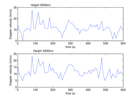
Figure 1: Doppler velocity time series at third ($\sim$ 5200 km) and fourth ($\sim$ 5900 km) heights in the spicule I. The time interval between consecutive measurements is $\sim$ 8 s.

We show a spectroscopic evidence of wave propagation in the chromosphere in terms of Doppler velocity oscillations in time at particular heights of solar limb spicules.

2 Observation and data analysis

Observations have been carried out on the big (53 cm) coronagraph of Abastumani Astrophysical Observatory (instrumental spectral resolution and dispersion in H${\alpha}$ are 0.04 Å and 1 Å/mm correspondingly) in September 26, 1981 at the solar limb as height series beginning at 3800 km height from the photosphere and upwards (for details, see Khutsishvili 1986). Chromospheric H${\alpha}$ line was used to observe solar limb spicules at 8 different heights. The distance between neighboring heights was 1^′′ (which was the spatial resolution of observations), thus the distance $\sim$ 3800-8700 km above the photosphere was covered. The exposure time was 0.4 s at four lower heights and 0.8 s at higher ones. The total time duration of each height series was 7 s. The consecutive height series begins immediately. Therefore continuous time series of H${\alpha}$ spectra with interval of $\sim$ 7-8 s between consecutive measurements at each height can be constructed. The time series cover almost whole life time (from 7 to 15 min) of several spicules.

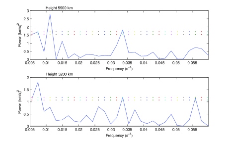
Figure 2: Power spectra of Doppler velocity oscillations in the spicule I at the heights of 5200 km (lower panel) and 5900 (upper panel) correspondingly. The dotted lines in both plots show 95.5$\%$ and 98$\%$ confidence levels. Here is the clear evidence of oscillations with the periods of 180 and 30 s at both heights.

Each H${\alpha}$ line profile from the time series was fitted to a Gaussian. Then temporal variations of the Gaussian center with respect to the photospheric reference line (4371 Å) have been studied at each heights for four different spicules. We have calculated the Doppler shifts, and consequently Doppler velocities, with 7-8 s interval at each heights in all spicules. Fig.1 shows the Doppler velocity time series at third ($\sim$ 5200 km) and fourth ($\sim$ 5900 km) heights in one of spicules. Then the spectral analysis of the time series at all heights has been carried out with the Discrete Fourier Transform (DFT). DFT enables to reveal oscillation periods with 20 - 250 s; the shorter periods are restricted due to an interval between consecutive measurements and the longer periods are restricted due to life times of spicules.

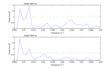
Figure 3: Power spectra of Doppler velocity oscillations in the spicule II at the heights of 5200 km (lower panel) and 5900 km (upper panel). The dotted lines show 95.5$\%$ and 98$\%$ confidence levels. This spicule shows the oscillations with the periods of 120 and 80 s at both heights.

3 Results

In this section, we present the results of DFT in four different spicules separately. Best fit of H${\alpha}$ line profiles to a Gaussian was found at third ($\sim$ 5200 km) and fourth ($\sim$ 5900 km) heights. The fit was relatively poor at lower and higher heights. Therefore calculated Doppler shifts are more confident at third and fourth heights. For this reason, we first show the results of DFT for these heights, then turn to general oscillatory phenomena at all heights.

3.1 Spicule I

Fig.2 shows the power spectra of Doppler velocity oscillations in the spicule I at the heights of 5200 km (below) and 5900 km (up). The dotted lines in both plots show 95.5$\%$ and 98$\%$ confidence levels respectively.

Most pronounced periods at the height of 5200 km are 180, 30 and 17 s (Fig.2, lower panel). However, 17 s period is probably suspicious as it is closer to the time interval between consecutive measurements ($\sim$ 7-8 s). So the oscillations of Doppler velocity with the periods of 180 and 30 s are more confident at this height. The upper panel shows the power spectrum at the height of 5900 km. Here the most pronounced periods are 180, 90 and 30 s. So the spicule oscillates with the periods of 30 and 180 s at both heights. The oscillation with the period of 90 s is also seen but preferably at the higher height (but note the small peak at the lower height as well).

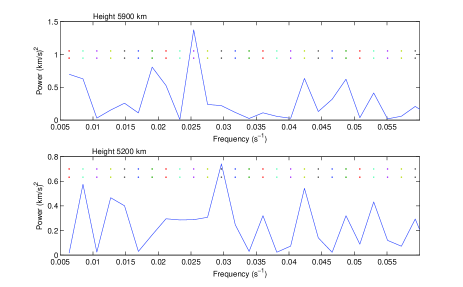
Figure 4: Power spectra of Doppler velocity oscillations in the spicule III at the heights of 5200 km (lower panel) and 5900 km (upper panel). The dotted lines show 95.5$\%$ and 98$\%$ confidence levels. This spicule oscillates with $\sim$ 35 s period at both heights.

3.2 Spicule II

Fig.3 shows the power spectra of Doppler velocity oscillations in the spicule II at the heights of 5200 km (lower panel) and 5900 km (upper panel). The dotted lines again show 95.5$\%$ and 98$\%$ confidence levels.

We see two clear oscillation periods of 120 and 80 s at both heights. Both periods are above 98$\%$ confidence level. There is some evidence of $\sim$ 50 s period at the height of 5200 km, but just below of 95.5$\%$ confidence level.

3.3 Spicule III

Fig.4 shows the power spectra of Doppler velocity oscillations in the spicule III at the heights of 5200 km (lower panel) and 5900 km (upper panel).

The spicule shows the oscillations with 37 s period at the height of 5200 km and with 35 s period at the height of 5900 km. Hence, the spicule oscillates with the period of $\sim 35$ s at both heights.

3.4 Spicule IV

Fig.5 shows the power spectra of Doppler velocity oscillations in the spicule IV at the heights of 5200 km (lower panel) and 5900 km (upper panel).

Clear oscillation periods in this spicule at both heights are $\sim$ 110 and $\sim$ 40 s. There is the evidence of oscillations with 30 s, but just below of 95.5$\%$ confidence level.

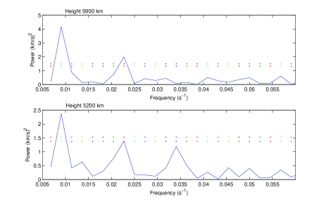
Figure 5: Power spectra of Doppler velocity oscillations in the spicule IV at the heights of 5200 km (lower panel) and 5900 km (upper panel). The dotted lines show 95.5$\%$ and 98$\%$ confidence levels. The periods of $\sim$ 110 and $\sim$ 40 s are most pronounced at both heights.

3.5 All oscillatory periods above 95.5$\%$ confidence level

Now let present the results of DFT for all 32 time series; i.e. at 8 different heights in 4 different spicules.

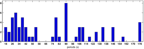
Figure 6: Histogram of all oscillation periods which are above 95.5$\%$ confidence level. The horizontal axis shows the oscillation periods in seconds, while the vertical axis shows the number of corresponding periods.

Fig.6 shows a histogram of all oscillation periods which are above 95.5$\%$ confidence level. The histogram reveals interesting properties of oscillatory periods in spicules. Almost half of the oscillatory periods are located in the range of 18-55 s, which have been suggested by Kukhianidze et al. in the paper I. Another interesting range of oscillatory periods is 75-110 s, with the clear peak at the period of 90 s. Note, the interesting peak at 178 s period as well, which is the clear evidence of well known 3 min oscillations.

In order to show spatial locations of oscillations we plot a Fourier power (expressed in confidence levels) as a function of frequency and heights for spicules II (Fig. 7, upper panel) and IV (lower panel). There is the clear evidence of persisted oscillations along whole length of both spicules. The plot of the spicule II shows the long white feature (feature A) located just above the frequency 0.01 s^-1. This is the oscillation with the period of $\sim$ 80 s found at third and fours heights (see subsection 3.2). The oscillation persists along whole spicule and is a signature of either standing or propagating wave pattern. The most pronounced feature (feature B) on the plot of the spicule IV is long light trend located just above the frequency of 0.02 s^-1 and persisted along almost whole spicule. This is the oscillation with period of 44 s (the same period was found at third and fourth heights; see subsection 3.4). Thus there is the wave pattern with $\sim$ 40-45 s period in the spicule IV. However, it must be mentioned again that only the oscillations at third and fourth heights have high confidence due to good fit of line profile to a Gaussian.

4 Discussion

Time series of H${\alpha}$ spectra in solar limb spicules show the clear evidence of Doppler shift oscillations, which probably are caused due to oscillations in line of sight velocity. Spicules have almost vertical direction at the solar limb, therefore the velocity is probably transversal to spicule axes. However, longitudinal oscillations also can not be ruled out if spicule axes are tilted from the vertical. It is clear that the oscillations in Doppler velocity can be caused due to wave propagations in spicules.

4.1 Wave propagation in spicules

Photospheric granulation is often suggested as a source for wave excitations in anchored thin magnetic tubes (Roberts 1979; Spruit 1981; Hollweg 1981; Hasan & Kalkofen 1999; Mishonov et al. 2007). The waves may propagate along the tubes towards the corona carrying energy and momentum. The tubes may guide spicule material at the same time. Therefore the wave propagation in the chromosphere may be traced through spicule dynamics. Magnetic tubes may guide three different types of waves: kink, sausage and torsional Alfvén waves. Some of these waves may cause the observed Doppler shift oscillations. Torsional Alfvén waves in thin tubes may lead to periodic non-thermal broadenings of spectral lines, but not to Doppler shift oscillations (Zaqrashvili 2003; Zaqarashvili and Murawski 2007). Sausage waves cause oscillations mainly in a line intensity due to density variations. However, the longitudinal velocity field of sausage waves may lead to the Doppler shift variations if tube axes are significantly tilted from the vertical. But the main contributor into Doppler shift oscillations at the solar limb probably are kink waves, which oscillate transverse to the tube axis. We argue that the back and forth transversal motions of vertical tube axis at the solar limb due to the propagation of kink waves is most plausible source for observed Doppler shift oscillations in spicules (Kukhianidze et al. 2005).

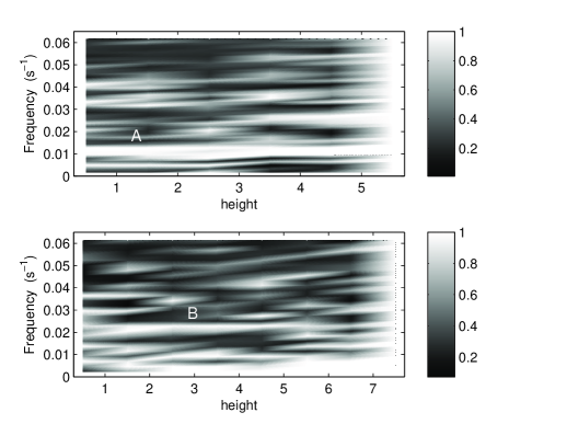
Figure 7: Fourier power expressed in confidence levels as a function of frequency and heights for the spicules II (upper panel) and IV (lower panel). Light points correspond to higher power and dark points correspond to lower one. The label 1 on the power scale (right plots) corresponds to the 100$\%$ confidence level. On the upper plot, we see long light feature located just above the frequency 0.01 s^-1 (feature A). On the lower plot, there is another long feature (feature B) located above the frequency 0.02 s^-1.

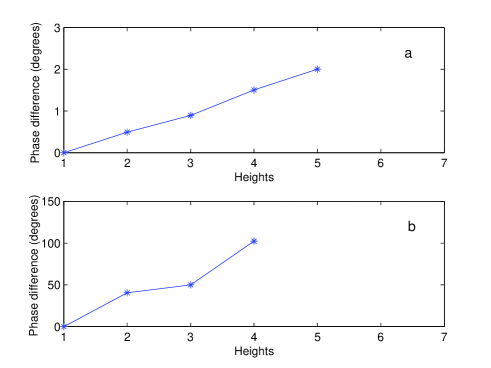
Figure 8: Relative Fourier phase as a function of heights for (a)$\sim$ 80 s period oscillation in spicule II (feature A on the upper panel of Fig.7) and (b) 44 s period oscillation in spicule IV (feature B on the lower panel of Fig.7).

Photospheric granulations may excite waves in anchored magnetic tubes with two different time scales. The first time scale can be similar to life-times of granular cells which gives wave periods of $\sim$ 5-10 min. The second time scale can be related to spatial scales of granular cells i.e. waves are excited with wave lengths corresponding to cell spatial dimensions ($\sim$ 200-1000 km). Then these waves may have periods of 20-100 s corresponding to typical photospheric wave speed $\sim$ 10 km s^-1 (both sound and Alfvén speeds probably have similar values in the photosphere). Fig.6 shows that more than 2/3 of oscillation periods are located in the range of 20-100 s, which clearly indicates to the granular origin of the waves. It is seen that the periods are split into two different ranges: 20-55 and 75-110 s. The reason of this phenomenon is not clear. There are two potential candidates for this splitting: either an unknown scaling of granular cells or fast and slow modes in thin tubes. The first case implies the scaling of granular cells into two different ranges of 200-500 and 800-1100 km, which is not known to our knowledge (however probably it is interesting to look into this problem in future). The second case implies the propagation of fast and slow waves in spicules. There are two different characteristic speeds of wave propagation in a magnetic tube embedded in a field-free environment; kink and tube speeds (Edwin and Roberts 1983)

$$c_{k}=c_{A}\sqrt{{{\rho_{0}}\over{\rho_{0}+\rho_{e}}}},\,\,\,c_{T}={{c_{0}c_{A}}\over{\sqrt{c^{2}_{A}+c^{2}_{0}}}},$$ (1)

where

$$c_{A}={B_{0}\over{\sqrt{4\pi\rho_{0}}}},\,\,\,c_{0}=\sqrt{{\gamma p_{0}}\over{\rho_{0}}}$$ (2)

are the Alfvén and sound speeds inside the tube respectively. Here $p_{0}$, $\rho_{0}$, $B_{0}$ are the pressure, the density and the magnetic field inside the tube, $\rho_{e}$ is the density outside the tube and $\gamma$ is the ratio of specific heats. Fast waves propagate with a phase speed close to the kink speed, while slow waves propagate with the tube speed. The density is much higher inside the spicule than outside, therefore the kink speed is close to the Alfvén speed. Let suggest that the Alfvén speed is three times more than the sound speed in spicules at observed heights (4000-8000 km) i.e. $c_{A}=3c_{0}$, then it implies $c_{k}\approx 3c_{T}$. Then the fast waves propagate three times faster than the slow waves. So if both waves are excited with the similar wave length then the period of fast waves must be three times shorter than that of slow waves. It is intriguing that the ranges 20-55 and 75-110 s have similar relation. Then the oscillations with 20-55 s period can be caused by the propagation of fast waves, while the oscillations with 75-110 s can be due to the slow waves. It is an interesting fact, that the oscillations with 75-110 s have significant power, even more than ones with shorter period. The oscillations may be signature of periodic vertical flows excited by the resonant buffeting of granular cells (Roberts 1979). In this interesting paper, Roberts suggested that the quasi-periodic external buffeting of granules on magnetic tubes may lead to periodic resonant vertical flows just as squeezing of a hosepipe drives a jet of water. The period of the external forcing was taken as about 5 min corresponding to mean life-time of granules. Consequently, resonant periodic flows must propagate with the tube speed and have the same $\sim$ 5 min period. However, there are usually 3-4 granular cells in the neighborhood of each photospheric vertical tube, which cause quasi-periodic squeezing of the tube. Then, the mean period of external forcing will be 3-4 times shorter than mean life time of granules. Consequently, the resonant periodic flows will have 80-100 s period, which surprisingly coincides to the observed periods. This phenomenon needs more vigorous analysis as it may deal with spicule formation mechanism, but it is out of scope of this paper.

Another interesting result is the clear peak at the period of 178 s (Fig.6), which probably indicates to oscillations with a period of 3 min. Thus the 3-min oscillations may penetrate up to the heights of 4000-8000 km. It is interesting to check if 5-min oscillations are presented in these heights. Unfortunately, statistical search of this period in our data is restricted due to life times of spicules.

It is particularly important to understand whether the oscillations are due to propagating or standing wave patterns. There are only 7-8 spatial points (corresponding to each heights) in our data, therefore to infer the phase propagation is not easy. In the paper I, we presented an illustrative example of phase propagation, but it needs more vigorous treatment. The wave propagation can be revealed through the variation of Fourier phase with position (Molowny-Horas et al. 1997). Unfortunately, using the method in our data is complicated as the oscillations have high confidence only at two heights (third and fourth ones). The oscillations at other 6 heights are not very confident due to poor fit of line profile to Gaussian. However, some rough estimations still can be made. We calculated the relative Fourier phase between heights for most pronounced features (features A and B) of Fig.7. Fig.8 shows the relative Fourier phase as a function of heights for (a) the feature A and (b) the feature B. There is almost no phase difference between oscillations at different heights for the feature A, which probably indicates a standing-like wave pattern with period of $\sim$ 80-90 s. On the contrary, there is the significant linear phase shift on the plot (b), which indicates a propagating pattern with period of $\sim$ 40-45 s. So the spicule II shows the standing-like pattern (or wave propagation almost along line of sight, which seems unlikely) and the spicule IV shows the propagation pattern. The propagation speed for the feature B can be roughly estimated. The wave length can be given as (Molowny-Horas et al. 1997)

$$\lambda={{2\pi}\over{\Delta\phi}}\Delta s,$$ (3)

where $\Delta\phi$ and $\Delta s$ are phase difference and distance between first and last points. Then it gives the upper limit for wave length as $\sim$ 6000 km. The actual wave length will be shorter if spicule is tilted from the vertical. For the 35⁰ tilt (Trujillo Bueno et al. 2005) the actual wave length is 4800 km. Then the phase speed of the feature B (with period of 44 s) can be estimated as

$$\sim 110\,\,{\rm km\cdot s}^{-1},$$ (4)

which is near the kink speed in the chromosphere. Thus, the feature B is probably due to the kink wave propagation in the spicule IV. The origin of the feature A is controversial. The oscillations are almost in phase at 5 different heights, which indicates to a standing-like pattern. The pattern can be formed due to the reflection of slow tube waves at the transition to the high-temperature corona. But the phase difference analysis is not very confident in our case, therefore the results can be spurious. Future detailed observations are necessary to confirm the phenomenon.

4.2 Spicule seismology

Observed waves can be used to infer plasma parameters inside spicules. The method called as coronal seismology is widely used in coronal loops (Nakariakov and Ofman 2001) and prominences (Ballester 2006).

In paper I we reported periodical distributions of H${\alpha}$ Doppler velocity with height. The spatial distribution has been explained in terms of kink wave propagation from the photosphere towards the corona. The wave length was estimated as ${\sim}3500$ km. Then we may calculate wave phase speed with the help of observed oscillation period, which enables to estimate a magnetic field strength in spicules. Recently, Singh and Dwivedi sing (2007) estimated a magnetic field of 10-26 G in spicules. They used the observed wave length from the paper I and the oscillation period of 1 min from Nikolsky and Platova nik (1971).

Fig.6 shows that most expected periods are $\sim$ 35 s and 90 s. Then the phase speed can be estimated either as $\sim$ 100 km s^-1 or $\sim$ 40 km s^-1. Both of them are higher than the adiabatic sound speed for a temperature of $\sim$ 15 000 K at height of $6000$ km (Beckers 1972), which gives $\sim$ 20 km s^-1. Therefore we argue that observed spatial periodicity in Doppler velocity with ${\sim}3500$ km (paper I) is caused by the propagation of kink waves with the period of 30-40 s. Then the kink speed in spicules at the heights of 3800-8700 km from the photosphere can be estimated as

$$c_{k}=90-115\,\,{\rm km\cdot s}^{-1}.$$ (5)

Note, that the Fourier phase difference, roughly estimated for the oscillation in spicule IV (feature B), also gives the similar value of the phase speed ($\sim$ 110 km/s, see previous subsection).

As a plasma density is much higher inside spicules than outside, then the kink speed is almost the Alfvén speed. Expected electron density in spicules at the height of 6000 km $8.9\cdot 10^{10}$ cm^-3 (Beckers 1972) gives the plasma density of $\rho_{0}\approx 1.4\cdot 10^{-13}$ g${\cdot}$cm^-3. Then, using the kink speed (5), we may estimate the magnetic field strength in spicules at the height of 6000 km as

$$B_{0}=12-15\,\,{\rm G}.$$ (6)

This is in a good agreement with recently estimated magnetic field strength in quiet-Sun spicules ($\sim 10$ G), which was obtained by spectropolarimetric observations of solar chromosphere in the He I $\lambda$10830 (Trujillo Bueno et al. 2005).

4.3 Some critical points

However, there are some critical points in interpretations of observational data.

1. Fine structure of spicules: it is quite possible that spicules are consisted of several thinner magnetic tubes with 100-200 km diameter and this fine structure is not resolved due to the spatial resolution of observations ($\sim$ 1 arc sec). Then each spicule may consist of several micro spicules. Each micro spicules may oscillate in its own way, which complicates the spectral analysis of integrated Doppler shift.

2. Line of sight effect of several spicules: some spicules show a multi-component structure (i.e. several spicules are located close together along a line of sight) mostly at lower heights, which may give the impression of a velocity shift (Xia et al. 2005). Therefore here only the spicules with well defined single-component structure were chosen, however the line of sight problem can not be completely excluded.

5 Conclusion

Here we analysed the old H${\alpha}$ spectra taken on the coronagraph of Abastumani Astrophysical Observatory in solar limb spicules. The time series include whole life times of four different spicules at 8 different heights covering 3800-8700 km above the photosphere (totally 32 time series). After DFT of the time series we conclude:

• Doppler velocities of spicules undergo oscillations with periods of 20-110 s;

• there are two different ranges of periods; almost half of the oscillatory periods are located in the range of 20-55 s and almost one third of oscillatory periods are located in 75-110 s;

• most pronounced oscillation periods are $\sim 35$ and $\sim 90$ s;

• there is an interesting peak at 178 s period, which is clear evidence of 3-min oscillations at the heights of 3800-8700 km (detection of 5-min period in our data is restricted due to life times of spicules);

• we suggest that the oscillations are caused due to wave propagations in the chromosphere;

• the waves or periodic flows likely are generated in the photosphere by granular cells;

• the two different ranges of periods can be explained either due to fast and slow waves or due to some unknown spatial scaling of granular cells;

• observations can be used to infer plasma parameters in spicules, i.e. spicule seismology;

• estimated magnetic field strength in spicules is $12-15$ G at the height of $\sim$ 6000 km above the photosphere.

However, some problems may arise in interpretations of observational data related to spicule fine structure or multi-component nature, which may lead to the impression of the velocity shift (Xia et al. 2005). Therefore future detailed spectroscopic observations with higher spatial resolutions are needed to confirm high frequency wave propagations in the chromosphere.

6 Acknowledgements

The work was supported by the grant of Georgian National Science Foundation GNSF/ST06/4-098. A part of the work is supported by the ISSI International Programme ”Waves in the Solar Corona”. We thank Prof. Kiladze for helpful comments and the referee for stimulating suggestions.

References

- (1) Ballester, J.L., 2006, Space Science Rev., 122, 129
- (2) Beckers, J.M., 1972, ARA&A, 10, 73
- (3) DeForest, C.E., 2004, ApJ, 617, L89
- (4) De Pontieu, B., Erdélyi, R. and de Wijn, A.G., 2003, ApJ, 595, L63
- (5) De Pontieu, B., Erdélyi, R. and James, S.P., 2004, Nature, 430, 536
- (6) Edwin, P.M. and Roberts, B., 1983, Solar Phys., 88, 179
- (7) Hasan, S.S. and Kalkofen, W., 1999, ApJ, 519, 899
- (8) Katsiyannis, A.C., Williams, D.R., McAteer, R. T. J. Gallagher, P. T., Keenan, F. P. and Murtagh, F., 2003, A&A, 406, 709
- (9) Khutsishvili, E., 1986, Solar Phys. 106, 75
- (10) Kukhianidze, V., Zaqarashvili, T. V. and Khutsishvili, E., 2005, Proceedings of the 11th European Solar Physics Meeting ”The Dynamic Sun: Challenges for Theory and Observations”, Leuven, Belgium, Eds. D. Danesy, S. Poedts, A. De Groof and J. Andries (ESA SP-600), 64
- (11) Kukhianidze, V., Zaqarashvili, T. V. and Khutsishvili, E., 2006, A&A, 449, L35 (Paper I)
- (12) Kulidzanishvili, V.I. and Zhugzhda, Y.D., 1983, Solar Phys. 88, 35
- (13) Hollweg, J.V., 1981, Solar Phys. 70, 25
- (14) Mishonov, T.M., Maneva, Y.G. and Hristov, T.S., 2007, J. Atmosph. and Solar-Terrestrial Phys., (in press)
- (15) Molowny-Horas, R, Oliver, R., Ballester, J.L. and Baudin, F., 1997, Solar Phys., 172, 181
- (16) Nakariakov, V.M. and Ofman, L., 2001, A&A, 372, L53
- (17) Nikolsky, G.M. and Platova, A.G., 1971, Solar Phys. 18, 403
- (18) Roberts, B. 1979, Solar Phys. 61, 23
- (19) Singh, K.A.P. and Dwivedi, B.N., 2007, New Astronomy, 12, 479
- (20) Spruit, H.C. 1981, A&A, 98, 155
- (21) Sterling, A.C., 2000, Solar Phys., 2000, 196, 79
- (22) Trujillo Bueno, J., Merenda, L., Centeno, R., Collados, M., Landi Degl’Innocenti, E., 2005, ApJ, 619, L191
- (23) Xia, L.D., Popescu, M.D., Doyle, J.G. and Giannikakis, J., 2005, A&A, 438, 1115
- (24) Zaqarashvili, T.V. and Roberts, B., 2002, Phys. Rev. E 66, 026401
- (25) Zaqarashvili, T.V., 2003, A&A, 399, L15
- (26) Zaqarashvili, T.V. and Murawski, K., 2007, A&A, 470, 353
- (27) de Wijn, A.G., Rutten, R.J., and Tarbel, T.D., 2005, A&A, 430, 1119
- (28) Wunnenberg, M., Kneer, F., and Hirzberger, J., 2002, A&A, 395, L15