Three-dimensional MHD simulation of expanding magnetic flux ropes

Abstract

Three-dimensional, time-dependent numerical simulations of the dynamics of magnetic flux ropes are presented. The simulations are targeted towards an experiment previously conducted at CalTech (Bellan, P. M. and J. F. Hansen, Phys. Plasmas, 5, 1991 (1998)) which aimed at simulating Solar prominence eruptions in the laboratory. The plasma dynamics is described by ideal MHD using different models for the evolution of the mass density. Key features of the reported experimental observations like pinching of the current loop, its expansion and distortion into helical shape are reproduced in the numerical simulations. Details of the final structure depend on the choice of a specific model for the mass density.

I Introduction

Magnetic fields play an important role for the structure and the dynamical behavior of the solar atmosphere. Well-known examples for structural features found on a variety of spatial scales are helmet streamers (bib:wiegelmann, ), sunspots, coronal loops and filaments, while flares, loop eruptions and coronal mass ejections are dynamical phenomena related to magnetic energy release (bib:aschwanden, ). The importance of the magnetic field structure and its evolution has prompted a lot of theoretical investigation in the past. For example, Török et al. (bib:kliem, ) use numerical simulations to study a scenario for loop eruptions due to kink mode instabilities, using the loop model by Titov and D moulin (bib:titov-demoulin, ).

An entirely different approach to study the evolution and creation of magnetic signatures found in the solar corona is the use of laboratory experiments. Bellan and Hansen report from an experiment which is considered a laboratory model for Solar prominence eruptions bib:bellan2000 ; bib:bellan2001 , and a similar experiment (“FlareLab”) has recently been set up at Ruhr-Universität Bochum. In the latter, the long term goal is to study a variety of magnetic field configurations and to employ extended plasma diagnostics.

Fig. 1 shows a crude sketch of these two experiments: A horse shoe magnet is mounted below the bottom plate of a vacuum chamber, producing an arc-shaped field inside the vessel. Two electrodes in the vicinity of the magnet poles are connected to a capacitor bank. In the experiment, hydrogen gas is puffed into the chamber shortly before the capacitor voltage is connected to the electrodes. A plasma arc is created by ionisation of the hydrogen, causing the voltage to break down and the capacitors to be discharged. The evolution of this arc is then followed by means of a fast camera in order to study the dynamics that follow from the internal magnetic forces. Images from different stages of the discharge process as published in (bib:bellan2000, ) indicate that the arc pinches in cross-section and expands as a whole on the scale of a few microseconds. At a later stage, it gets further deformed and assumes a helical shape. A corresponding photograph recently taken from “FlareLab” is shown in Fig. 2.

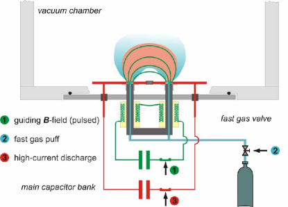
Figure 1: Sketch of the initial experimental setup used by Bellan (bib:bellan2001, ) and in “FlareLab” at Bochum Universität.

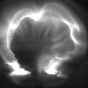
Figure 2: Image taken from the “FlareLab” experiment at $7\mu s$ after ignition. The plasma arc has already expanded to approximately three times its initial radius and helical distortions are clearly visible.

Later, this basic experimental setup has been modified by Bellan et al. to include an additional magnetic field component with field lines that cover the entire filament structure at a right angle. Using this modified setup, it was demonstrated that the “strapping” field component can inhibit the arc expansion (bib:bellan2001a, ). Also, the interaction between two current arcs has been studied in an other extension of the basic configuration (bib:bellan2arcs, ).

This experimental approach offers an attractive way to gain insight into the dynamical behavior of magnetic structures, because it opens a way to analyze details of the dynamics through the measurement of physical quantities like the magnetic field, which are not directly accessible in the solar context. Apart from this, the possibility to control and selectively modify parameters like boundary- and initial conditions allows systematic investigations and the test of theoretical models or comparison with computer simulations. However, a number of questions arise concerning the interpretation of the experimental observations and its relevance for solar physics: First of all, it is not clear if the model of magneto-hydrodynamics (MHD), which seems appropriate in the solar context and has been adopted for the interpretation of experimental findings (bib:bellan2000, ), can be applied to the experiment without limitations. While the plasma arc itself may be highly ionized, there is no indicaction available from the experiment concerning the electron density off the regions of highest luminosity. Therefore, it is unclear if, for instance, the “frozen-flux” principle applies in those surrounding regions and what the consequences of any “non-ideal” behavior would be.

In an attempt to obtain a better understanding for the dynamical evolution of the plasma arc, we have carried out a number of computations which aim at simulating the plasma dynamics in the experiment. Using the model of ideal MHD, we can address the question whether experimental results in fact are compatible with that model, and to which extent it is capable of reproducing the observed structures. In addition, detailed data is available about relevant quantities like the magnetic field, electric current and plasma flow. It should be stressed that these simulations are directed at the laboratory experiment alone, and no attempt is made at this point to draw conclusions for prominence dynamics in the solar atmosphere.

II Model and Numerical Treatment

We employ the model of ideal MHD,

$$\frac{\partial\rho}{\partial t} = -\nabla\cdot\left(\rho\vec{v}\right)+S$$ (1)

$$\frac{\partial\vec{v}}{\partial t} = -\left(\vec{v}\cdot\nabla\right)\vec{v}+\frac{\vec{j}\times\vec{B}}{\rho}-\frac{\nabla p}{\rho}+\nu\Delta\vec{v}$$ (2)

$$\frac{\partial\vec{B}}{\partial t} = \nabla\times\left(\vec{v}\times\vec{B}\right)$$ (3)

$$\nabla\times\vec{B} = \mu_{0}\vec{j}.$$ (4)

Here, $\rho$, $\vec{v}$, $\vec{B}$, $p$ and $\vec{j}$ denote the mass density, plasma bulk velocity, magnetic field, thermal pressure and electric current density, respectively. A homogeneous kinematic viscosity, $\nu$, is included for reasons of numerical stability. In (1), a yet unspecified source term $S$ allows the model to deviate from plasma mass conservation. As described below in detail, this term is used in order to implement different models for the plasma density in our simulations, namely i) mass conservation, $S=0$, ii) a homogeneous density, $\rho=\rho_{0}$ iii) a fixed Alfvén velocity, $\rho\propto|\vec{B}|^{2}$ and iv) a crude model for ionization and recombination (case 4 below). These models are only partly motivated on physical grounds, but we note that Eq. (2) is written in non-conservative form and hence remains consistent with (1) even for $S\neq 0$ if it is assumed that plasma created according to $S$ has the same velocity as the existing plasma population. For an ionization term, this is the case if the neutral gas component moves at the same velocity $\vec{v}$ as the charged species. To close Eqs. (1)–(3), we assume an isothermal plasma, $p=T\rho$, in case i) (i.e. mass conservation) and $p=0$ in all other cases.

All quantities are normalized to a typical value of the magnetic field strength, $B_{0}$, a length scale, $L_{0}$, and the Alfvén velocity, $v_{A}=B_{0}/\sqrt{\mu_{0}\rho_{0}}$ with a typical value for the mass density, $\rho_{0}$. A normalization time scale follows as $t_{0}=L_{0}/v_{A}$, and the relationship of these scales with the experimental setup are described below.

II.1 Initial conditions

At $t=0$, the plasma is assumed to be at rest, $\vec{v}=0$, with a prescribed density distribution according to one of the specific density models. Hence, we make no attempt to describe the ionization stage of the experiment, but rather start with a configuration that contains highly conducting plasma in the entire domain.

A cartesian coordinate system is used in which the plasma chamber wall that contains the two electrodes lies in the plane $z=0$, and the electrodes themselves are located at $\pm R\vec{e}_{y}$.

The initial magnetic field consists of two parts: The contribution from the horse shoe magnet in the experiment is modeled by the field $\vec{B}_{d}(\vec{x})$ created by two virtual magnetic dipoles located outside the domain at positions $\vec{x}_{\pm}=\pm R\vec{e}_{y}-R\vec{e}_{z}$, i.e. “below” the electrodes. They are assumed to carry dipole momenta $\vec{m}_{\pm}=\pm m\vec{e}_{z}$ with $m$ chosen such that the field at the electrode positions is normalized, $|\vec{B}_{d}(\pm R\vec{e}_{y})|=1$. It follows that

$$\vec{B}_{d}(\vec{x})=\sum_{i=\pm}\frac{3\left(\vec{m}_{i}\cdot\left(\vec{x}-\vec{x}_{i}\right)\left(\vec{x}-\vec{x}_{i}\right)\right)-\vec{m}_{i}\left|\vec{x}-\vec{x}_{i}\right|^{2}}{\left|\vec{x}-\vec{x}_{i}\right|^{5}}.$$ (5)

A second initial magnetic field component, $\vec{B}_{c}(\vec{x})$, mimics the field related to the plasma current in the early stage of the discharge. A quantitative model for $\vec{B}_{c}$ is constructed by means of a vector potential $\vec{A}_{c}(\vec{x})$ with $\vec{B}_{c}(\vec{x})=\nabla\times\vec{A}_{c}(\vec{x})$, and the choice of $\vec{A}_{c}(\vec{x})$ is motivated by the assumptions that i) the initial current is approximately localized around the half-circle in the plane $x=0$ which connects the electrodes, and ii) the direction of $\vec{A}_{c}$ coincides with the direction of $\vec{B}_{d}$ because the ring current will roughly follow those field lines. With $\vec{e}_{d}(\vec{x}):=\frac{\vec{B}_{d}(\vec{x})}{|\vec{B}_{d}(\vec{x})|}$ given from the dipole field model above, we choose

$$\vec{A}_{c}(\vec{x})=A_{0}\;e^{-(|\vec{x}|-R)^{2}/\delta^{2}}\;e^{-x^{2}/\delta^{2}}\;\vec{e}_{d}(\vec{x})$$ (6)

The exponentials localize the magnetic structure on a scale of $\delta=0.625$ around the ring of radius $R$ in the $y$-$z$-plane. The amplitude $A_{0}$ is determined from the condition that the maximum of $|\vec{B}_{c}|$ in the bottom plane $z=0$ is $\max_{z=0}(|\vec{B}_{c}|)=3$, which roughly corresponds to the ratio of the current-induced magnetic field to the horse-shoe magnetic field magnitude taken at the position of the electrodes as estimated for the experimental setup (see below).

At this point, we would like to stress that the resulting initial magnetic field, $\vec{B}(\vec{x},t=0)=\vec{B}_{d}(\vec{x})+\nabla\times\vec{A}_{c}(\vec{x})$, is not force-free. Even with a (small) thermal pressure term added, there is no force equilibrium at the start of the simulation, which is in accordance with the experiment. The aim here is, similar to the experiment, to investigate dynamical properties of the resulting evolution.

II.2 Density models

In the next section, we will describe results obtained from four simulation runs, all of which use the same initial magnetic field as described above, but differ in the treatment of the mass transport, i.e. in the specific realization of Eq. (1):

Case 1 - Mass conservation: Here, Eq. (1) is used as a continuity equation with $S=0$, describing mass conservation. More specifically, we use a homogeneous mass density $\rho=1$ as initial condition and specify the temperature as $T=1$. This model can be seen as the simplest choice possible that accounts for a consistent mass transport during the dynamical evolution of the system. Realizing that $|\vec{B}|\approx 3$ in the current filament, the resulting local plasma-$\beta$ is $2/|\vec{B}|^{2}\approx 0.2\ll 1$.

Case 2 - Fixed density: We keep $\rho=1$ fixed throughout the simulations, i.e. Eq. (1) is abandoned. As a consequence, sound waves are eliminated from the dynamics. This model is used in order to get an indication of the influence of the mass transport and pressure included in the previous case on the evolution.

Case 3 - Fixed Alfvén velocity: In this case, the mass density is continuously adjusted such that the Alfvén velocity is constant throughout the domain, i.e. $\rho(\vec{x},t)\propto|\vec{B}(\vec{x},t)|^{2}$. The interest for this study stems from the fact that the evolution might be treated as quasi-static (bib:bellan2000, ), which means that the Alfvén crossing times are small compared to the global evolution time scale. Setting $v_{A}$ to a constant value results in a homogeneous communication of Alfvénic disturbances.

Case 4 - Ionization/recombination model: Here, we implemented a simple model for the ionization by the electric current and chose the source term as

$$S=\Gamma_{i}\vec{j}^{2}+\Gamma_{r}(\rho-\rho_{0}).$$ (7)

The coefficients are set to $\Gamma_{i}=0.5$, $\Gamma_{r}=5$ and $\rho_{0}=1$ so that the time scales of ionization and recombination are comparable to the Alfvénic and convection time scales.

II.3 Numerical implementation

Equations (1)–(3), with a specific density model, are discretized by finite-differences on a cartesian grid and integrated as an initial value problem using a third order Runge-Kutta scheme. The numerical box covers $[-20,20]\times[-20,20]\times[0,40]$ in the $x-$, $y-$ and $z-$direction, respectively. Boundary conditions at $z=0$, i.e. the “bottom” plane, are such that $\vec{v}=0$ and $\vec{B}_{\perp}$ is linearly extrapolated. We use outflow boundary conditions, i.e. the ghost cell values are set to the first cell values within the domain. However, the simulated current filaments are well separated from those boundaries so that these conditions have no significant influence on the results.

In order to obtain sufficient spatial resolution of the current filament dynamics, we carried out mesh-adaptive computations with local refinement using the simulation code “racoon” (bib:racoon, ). Grid blocks of $16^{3}$ cells each are recursively refined up to a local resolution equivalent to $1024^{3}$, using a refinement criterion that compares the electric current density $|\vec{j}|$ with a critical value $j_{crit}$ that is determined from the existing local resolution. A typical grid layout is depicted in Fig. 3.

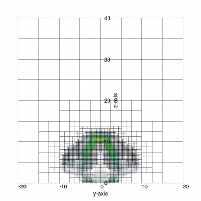
Figure 3: The full computational domain with the block distribution and the line-of-sight integrated electric current density, viewed parallel to the $x$-axis.

II.4 Scaling of experimental parameters

The model described above involves a number of normalization values for the MHD quantities. In order to allow a direct comparison with the experiments of Bellan et al. and “FlareLab,” we relate these values to physical parameters given in (bib:bellan2000, ) and estimates from the “FlareLab” experiment (not yet published).

With $L_{0}=16\;{\rm mm}$, the electrode spacing is $5L_{0}=8{\rm cm}$ which corresponds to the experimental value, and the entire domain covered in the computation is $64\times 64\times 64{\rm cm}$ which roughly corresponds to the dimensions of the plasma vessel. Taking $B_{0}=0.3\;{\rm T}$, which matches the horse shoe magnetic field at the electrodes in the “FlareLab” experiment, and assuming a hydrogen plasma of $n_{0}\approx 10^{20}\;{\rm m}^{-3}$, results in an Alfvén velocity of $v_{A}=6\cdot 10^{5}\;{\rm m/s}$ and an Alfvén crossing time of $t_{0}\approx 2.6\cdot 10^{-8}\;{\rm s}$. This value is small compared to the macroscopic evolution time scale of $\approx 1{\rm\mu s}$ reported for the experiment, but two things should be noted here: First, from experiment the detailed density distribution can only be estimated as the experiments still lack suitable diagnostics to measure this value. More importantly, the magnetic field strength drops off drastically with increasing distance from the magnet poles/current filament, and the filament length increases in time from its initial value of $\approx 10\;L_{0}$. Hence, the true Alfvénic travel time along the filament from one electrode to the other will be longer than $t_{0}$ and might reach the overall evolution time scale.

As for the magnitude of the initial magnetic field created by the plasma current, $\vec{B}_{c}$, we assume the entire discharge current of $I\approx 50\;{\rm kA}$ to be located in a channel of radius $\delta=0.625L_{0}=10{\rm mm}$. By Amp re’s law, this will create an azimuthal magnetic field of $B_{\varphi}=\mu_{0}I/2\pi\delta=1\;T\approx 3.3\;B_{0}$ on the channel surface. Hence, we chose the magnitude of $A_{c}$ in Eq. (6) such that $|\vec{B}_{c}|=3$ close to the electrode.

The viscosity in (2) is included for numerical stability of the simulations. It was necessary to use a normalized value of $\nu=0.01$ in cases 1 and 2 and an even larger value of $\nu=0.05$ in cases 3 and 4. These values might correspond to a significantly higher viscosity than the actual physical one of the experiment. However, not only is the latter largely unknown by value, but it is also questionable if the viscous term in the momentum equation provides a realistic description at all. Hence, we treat the viscosity as a purely numerical parameter necessary for stabilizing the computations.

III Simulation Results

The observations in the experiment are made with an optical CCD camera. It is obviously difficult, if not impossible, to unambiguously relate the luminosities of the images to plasma quantities, but we see it as a reasonably assumption that there exists a close correlation between the electric current density and the luminosity. Therefore, the simulation results presented here focus mainly on the current density evolution, and volume renderings of $|\vec{j}|$ are shown in the plots discussed below for comparison with the images taken by the laboratory camera. Further, a view perpendicular to the current arc is chosen, again to fit the camera’s perspective in the “FlareLab” set-up.

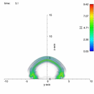
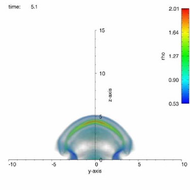
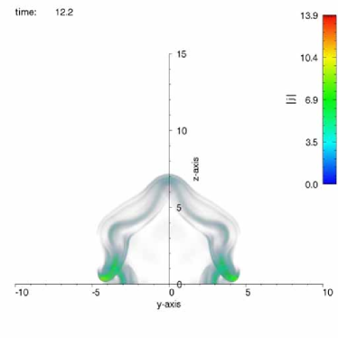
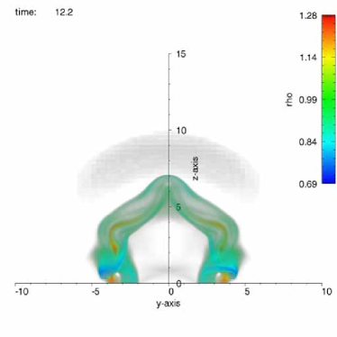
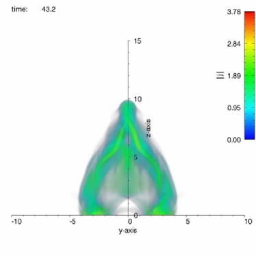
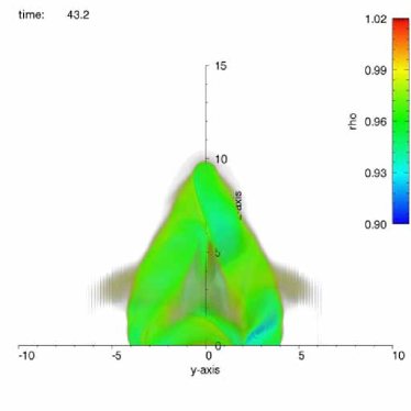
Figure 4: Electric current density $|\vec{j}|$ (left) and mass density $\rho$ (right) of simulation run 1 at times $t=5.1$ (top), $t=12.3$ (center) and $t=43.2$ (bottom).

Fig. 4 shows the spatial distributions of $|\vec{j}|$ and $\rho$ at three different times of simulation case 1, i.e. the run implementing mass conservation. Essential dynamical features can be observed on different time scales: Within the first Alfv n time, the current arc pinches to approximately half of its initial diameter. This effect can be determined from the plots taken at $t=5.1$: The current is more localized than in the initial configuration, and the mass density is enhanced in the arc center as a consequence of the compressional plasma motion. Accordingly, the density is reduced around the arc with minimum values of $\approx 0.53$. This deviation of mass density distribution from the initial homogeneous value corresponds to the formation of pressure gradients due to the assumption of isothermal plasma with normalized temperature $T=1$. It should be noted that the pinching is less pronounced close to the electrodes where the dipole magnetic field component is comparable in magnitude to the non-potential $\vec{B}_{c}$. Apart from this pinching, the arc as a whole has undergone an expansion from its original major radius $R=2.5$: The apex has risen to $z\approx 4.5$ and the curvature in the upper part of the arc is reduced compared to the original half-circle shape. Also, close to the electrodes, a more pronounced deformation of the current channel into helical shape is observed. Both, the expansion and the foot point deformation occur on the scale of several Alfv n times, i.e. slightly slower than the pinching. In the following evolution, the current structure and the mass density perturbation continue to expand (resp. times $t=12.2$ and $43.3$), causing the loop apex to rise to about $z=10$, i.e. four times its initial height. In the course of this expansion, the tendency of helical deformation manifests itself on the entire structure and grows in amplitude. Eventually, the upper part of the loop is entirely rotated out of the plane $x=0$ and intersects that plane at right angle with its apex (time $43.2$). Later, the expansion slows down and finally stalls shortly after the last frame shown in Fig. 4. After that, the structure actually starts to shrink slightly but finally comes to rest in a configuration close to the last one shown.

The qualitative interpretation of this sequence in terms of ideal MHD appears to be straight-forward: Recalling that the initial configuration is not in force balance, the current will pinch towards a force balance perpendicular to the center of the current tube. With the original diameter of $2\delta=1.25$ and an amplitude of the current-induced field of $|\vec{B}_{c}|=3$ and density $\rho\approx 1$, this process occurs on a time scale of $\approx 0.1$. The expansion of the arc can be interpreted as the response to the well-known “hoop force” caused by the arc curvature. As the arc follows this force, the curvature and the corresponding current density are reduced and the expansion slows down. In the vicinity of the foot points, the line-tying condition and the zero velocity boundary condition prevent the arc from following the expansion in the horizontal directions, and hence the arc looses its circular shape with its upper part merely rising upwards. Finally, we interpret the formation of helices at the foot points as kink modes and the fact that these modes develop fastest at the electrodes as a consequence of the different local Alvfén velocities: While the magnetic field is dominated by $\vec{B}_{c}$ on the entire arc, the mass density is considerably reduced to values around $0.5$ close to the electrodes in the early stage dynamics (cf. $\rho$ at $t=5.1$ in Fig. 4). Hence, the Alfvénic kink dynamics will be twice as fast as in the apex, where $\rho\approx 2$ as a consequence of the early pinching. This estimate is consistent with the fact that kinks become apparent at $t\approx 10$ at the apex, while they form already around $t\approx 5$ at the electrodes. At later stages, the entire structure relaxes into an approximately force-free state in which the internal twist of the magnetic field has been converted into a large-scale writhe.

Using the results of case 1 from above as a reference, we describe in the following the significant differences observed in the remaining simulation runs.

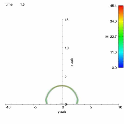
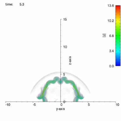
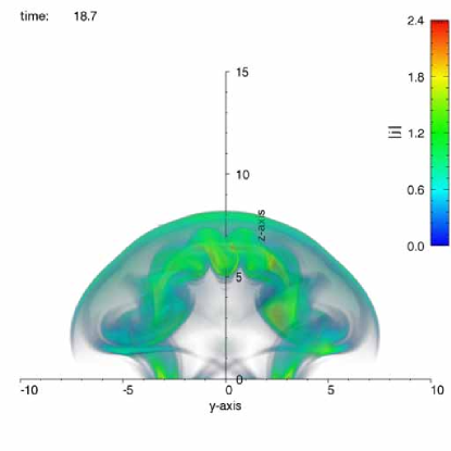
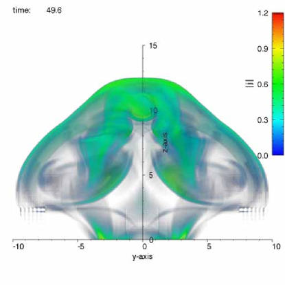
Figure 5: Electric current density $|\vec{j}|$ of simulation run 2 at times $t=1.5$, $t=5.1$, $t=18.7$ and $t=49.6$.

Fig. 5 displays the current structure of case 2 (“fixed density”) at different times. While the overall evolution is similar to case 1, some consequences of the constant mass density, and hence the absence of pressure forces, are readily visible. First of all, the maximum current density during the pinching phase is significantly larger than in case 1 ($\approx 45$ compared to $\approx 10$ at time $t\approx 1.5$), apparently because of the absence of restoring thermal pressure forces in case 2. Another consequence of the homogeneous mass density is that the kink formation in the apex region occurs already at $t\approx 5$, at the same time as it is observed close to the foot points. This homogeneity along the arc slightly alters the overall structure formation: While case 1 displayed an evolution from the foot points to the apex and from short wavelengths to larger scales, the development in case 2 is almost uniform along the arc. Small scale kinks occur early and grow in amplitude until the perturbation of the arc becomes almost stationary in shape, and only the slow expansion of the structure can be seen in the simulation. In particular, the pronounced rotation of the structure as a whole as seen in case 1 is absent here. Rather, the late stage can still be interpreted as a large current arc lying in the $x=0$-plane and continuing to expand.

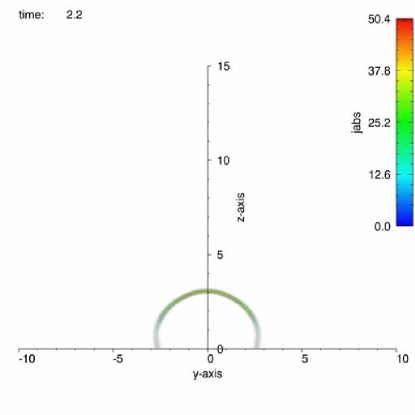
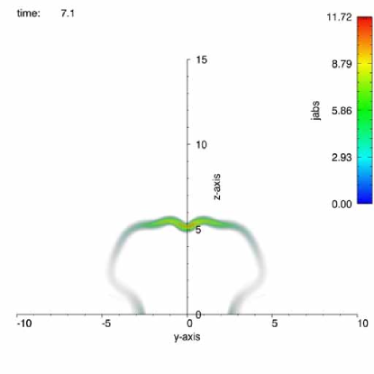
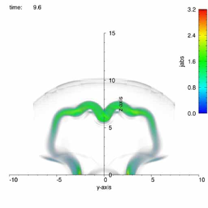
Figure 6: Electric current density $|\vec{j}|$ of simulation run 3 at times $t=2.2,7.2$ and $9.6$, respectively.

Fig. 6 shows that the evolution of the current structure in case 3 (“fixed Alfvén velocity”) resembles closely the results of case 2. The upper part of the arc flattens and forms kinks, however, the formation of kinks is constrained to the upper part of the arc and the “legs” remain almost unperturbed.

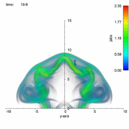
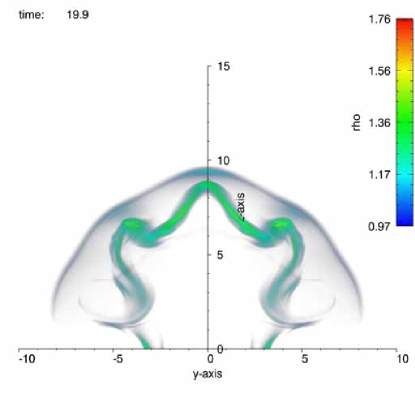
Figure 7: Electric current density $|\vec{j}|$ (left) and mass density (right) of simulation run 4, time $t=19.9$.

Finally, the inclusion of a simple recombination/ionization model in case 4 again leads to a slight differences in the resulting current system (Fig. 7), but the overall shape is still comparable to the previous cases, in particular to case 2.

Comparison with Experiment and Discussion

As noticed before, the experimental observations and the numerical simulations can only be compared on a qualitative level, not least because of the missing quantitative data from the experiment: It is not clear in which way the photographic luminosity originating from the neutral hydrogen emissions is related to the physical plasma parameters and fields. Based on the assumption that the electric current is the dominant source for ionization, and thus the plasma density and temperature will be well correlated to the current density, we choose to compare the laboratory images to $|\vec{j}|$ obtained from the numerical simulation.

Further fundamental differences between the experimental regime and the simulation model must be kept in mind: First of all, the model of ideal MHD is an idealized approach to the physics of the plasma discharge, in particular with respect to the degree of ionization, the ionization process during ignition, the role of collisions and possible kinetic or at least multi-fluid effects. In addition, the treatment of the boundaries and the coupling of the electrodes to the plasma is highly idealized. An other difference between model and experiment is that the total discharge current increases in time during the arc evolution, while the simulation boundary conditions imply a constant, prescribed current through the lower plane. Concerning the time scales, we note that a direct identification of simulation time with observed time scales is difficult because the fundamental plasma parameters of the experiment are currently only estimated.

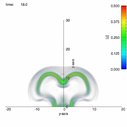
(a)
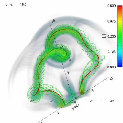
(b)

Figure 8: a) $|\vec{j}|$ from run similar to case 3 but with $\nu=0.1$ at time $t=18.0$. b) Perspective view of selected magnetic field lines (green), electric current lines (red) and $|\vec{j}|$ (grey shade) from the same run.

Keeping these limitations in mind, the computations reproduce key features of the laboratory results like the arc expansion and the kink formation. For example, by comparing Fig. 2 with the distributions of $|\vec{j}|$ from the four simulation runs, the qualitative agreement becomes evident. The moderate modifications of the density model that we employed in the four different runs lead to slightly different details in the arc dynamics as manifested, e.g. in the location, number and intensity of kinks. Asking which of these models can best reproduce the experiment, we observe that a characteristic feature there is the fact that the central region of the arc consistently gets bent downwards (see Fig.2). This fact has been reported by Bellan et al. bib:bellan2001 as well. In the simulations, we observe the same behavior in run 3 (constant Alfvén velocity) and we explain it by the fact that the mass density $\propto B^{2}$ assumes its largest values in the apex of the plasma arc. The reason for this is that the initial dipole field $\vec{B}_{d}$ is weakest there which leads to a relatively strong pinching effect and hence large values of $\vec{B}$. The large mass density close to the apex causes that part of the arc to lag behind during the arc expansion, leading to the characteristic dip.

We repeated the simulation of case 3 with an increased value for the viscosity ($\nu=0.1$ instead of the previous $\nu=0.05$) and achieved an even better agreement with the experimental pictures (Fig. 8 a). With this modification, the overall structure of the arc appears smoother compared to the previous run 3. The data of this high viscosity run has been used to produce a perspective view of the arc structure, showing magnetic field lines and electric current lines (Fig. 8 b). In this view, the overall structure of the arc as a helically distorted current channel becomes much more evident than from the axes-parallel views and shows an excellent agreement also with an image published in bib:bellan2001 .

Taking these findings together, we conclude that the present simulations represent a successful initial step to model the overall dynamics of the experiment in the framework of ideal MHD. Despite the fact that the present models contain a number of ad-hoc assumptions (like a specific density model, the presence of viscosity and a simple isothermal energy transport equation), the results are remarkably encouraging. For the future, we expect improved experimental diagnostics to give important additional information that in turn might lead to a more adequate theoretical and numerical description and hence to an even better agreement between both approaches.

Acknowledgments

Access to the JUMP multiprocessor computer at the FZ Jülich was made available through project HBO18. Part of the computations were performed on a Linux-Opteron cluster supported by HBFG-108-291. This work benefited from partial support through DFG-SO 380, DFG-GK 1051 and VH-VI-123.

References

- (1) Wiegelmann, T., K.Schindler and T. Neukirch, Sol. Phys., 180, 439, (1998).
- (2) Aschwanden, M., Physics of the solar corona: An introduction with problems and solutions Springer-Verlag (2007).
- (3) Török, T., B. Kliem and V. S. Titov, Astron. Astrophys., 413, L27 (2004).
- (4) Titov, V.S. and P. D moulin, Astron. Astrophys., 351, 707 (1999).
- (5) Bellan, P. M. and J. F. Hansen, Phys. Plasmas, 5, 1991 (1998).
- (6) Bellan, P. M. and J. F. Hansen, in: Proceedings of ISSS-6, Copernicus Gesellschaft (2001).
- (7) J. F. Hansen and P. M. Bellan, Astrophys. J. 563, L183 (2001).
- (8) J. F. Hansen, S. K. P. Tripathi, and P. M. Bellan, Phys. Plasmas, 11, 3177 (2004).
- (9) Dreher, J. and R. Grauer, Parallel Computing, 31, 913 (2005).