Inflating branes inside topological defects and periodic structures

Abstract

We study brane world models which contain local topological defects in the bulk and a $(3+1)$-dimensional inflating brane. We put the emphasis on new types of solutions that are periodic in the bulk radial coordinate and thus provide examples of “naturally compactified” brane worlds.

1 Introduction

The basic idea of brane worlds [1, 2, 3, 4, 5, 6, 7] is that our Universe is represented by a 4-dimensional space-time -the brane- embedded in a higher dimensional space -the bulk. This interpretation raises many challenges, the main one being the experimental signature revealing the extra dimensions. Natural questions are: how many extra dimensions are there and, if any, are they finite, i.e. compact or infinite.

If the extra dimension are large or even infinite, an appropriate mechanism has to be implemented in order to confine the fields and their interactions on the brane. Gravity as a property of space-time itself is naturally not confined to the brane but the fact that Newton’s law is valid down to scales of roughly one millimeter has to be taken into account. A possibility is that the space-time in the bulk is “warped” [5, 6].

Compact extra dimensions as they e.g. appear in Kaluza-Klein theory [8] or string theory [9] are implemented into the theory “by hand”. However, one could also think that “natural compactifications” are possible. Indeed, a few years ago in the study of the Einstein-Yang-Mills and Einstein-Yang-Mills-Higgs models in four space-time dimensions it was found that in the presence of a positive cosmological constant the space-time has a natural compactification for specific values of the cosmological constant [10].

In this paper, we investigate if similar results are available in the framework of brane world models. The three main ingredients for the models studied here are: (i) we have a non-vanishing bulk cosmological constant, (ii) there is a local topological defect residing in the bulk, the nature of which depends on the number of extra dimensions $n$: string-like for $n=2$, monopole for $n=3$ and (iii) the inflating brane is localised at the origin of the topological defect. Models containing these ingredients have been studied in detail in [11, 12], however, here we put the emphasis on periodic structures and give further details.

Note that our work is an extension of the work in [13], where brane worlds containing topological defects were studied. However, the branes were assumed to be static Minkowski branes. In [14], on the other hand, inflating branes were studied, but in a bulk without cosmological constant.

The paper is organised as follows: in Section 2 we describe the model and the ansatz for the metric. Some analytic solutions of the vacuum Einstein equations are presented in Section 3. The models containing matter fields in the bulk in the form of topological defects are presented in Section 4, where we also present our numerical results. We give our summary in Section 5.

2 The model

In this paper, we consider a $(3+1)$-dimensional brane in an $n$-dimensional space-time. The bulk contains either no matter fields at all (vacuum case) or a local topological defect. The action for this model reads:

$$S=\frac{1}{16\pi G_{n+4}}\int\sqrt{-g}(R+\Lambda_{n+4})d^{n+4}x+S_{bulk}$$ (1)

where $S_{bulk}$ is the action that describes the specific model and will be given in explicit form later in the paper. $G_{n+4}=\frac{1}{M_{*}^{n+2}}$ is the fundamental gravity scale with $M_{*}$ the $(n+4)$-dimensional Planck mass. $\Lambda_{n+4}$ denotes the bulk cosmological constant.

The general form of the non-factorisable metric that we consider in this paper is given by:

$$ds^{2}=M(r)^{2}ds_{4}^{2}+dr^{2}+L(r)^{2}d\Omega_{n-1}$$ (2)

where $ds_{4}^{2}$ describes the metric $g_{\mu\nu}^{(4)}$ of the $3$-brane. This 4-dimensional metric satisfies the 4-dimensional Einstein equations:

$$G_{\mu\nu}^{(4)}=8\pi G_{4}g_{\mu\nu}^{(4)}\ \ ,\ \ \mu,\nu=0,1,2,3\ .$$ (3)

The transverse space has rotational invariance, $r=\sqrt{\sum\limits_{k=1}^{n}x_{k}^{2}}$ describes the bulk radial coordinate, while $d\Omega_{n-1}$ denotes the line element associated with the $n-1$ angles $\Theta_{i}$, $i=1,..,n-1$ of the transverse space.

Throughout this paper, we study inflating branes and thus choose the following Ansatz for the brane metric:

$$ds_{4}^{2}=-dt^{2}+e^{2Ht}\left(d\tilde{x}_{1}^{2}+d\tilde{x}_{2}^{2}+d\tilde{x}_{3}^{2}\right)$$ (4)

with $H=\sqrt{\frac{\Lambda_{phys}}{3}}$, where $\Lambda_{phys}$ denotes the physical cosmological constant on the brane. $\tilde{x}_{1}$, $\tilde{x}_{2}$, $\tilde{x}_{3}$ are cartesian coordinates on the brane. The resulting Einstein equations are given in [12].

In this paper, we are interested in solutions that have metric functions which are periodic in the bulk radial coordinate $r$. These solutions appear for $\Lambda_{phys}>0$, so we restrict our discussions here to inflating branes.

3 Vacuum solutions

Here, we discuss the solutions of the resulting Einstein equations without matter fields in the bulk, i.e. $S_{bulk}=0$.

3.1 $n=2$

In the case of a two extra dimensions, it was noticed in [11] that the equations lead to the proportionality of the metric function $L$ to the derivative of $M$, $L\propto M^{\prime}$. The metric functions for the case of an inflating brane in a de Sitter bulk then read:

$$M(r)=\sqrt{\frac{80\pi G_{4}\Lambda_{phys}}{3\Lambda_{6}}}\sin\left(\sqrt{\frac{\Lambda_{6}}{10}}r\right)\ \ ,\ \ L(r)=L_{0}\cos\left(\sqrt{\frac{\Lambda_{6}}{10}}r\right)\ .$$ (5)

where $L_{0}$ is a constant.

This solution describes a space-time that can be interpreted as infinitely many copies of a finite space-time with length $2\pi/\sqrt{\frac{\Lambda_{6}}{10}}$. The finiteness of the space-time allows for a finite effective 4-dimensional Planck mass $M_{pl}$ [11].

Since the curvature invariants contain a term of the form $1/M^{2}$, this vacuum solution is singular at the origin $r=0$. We will see later in the paper that the presence of matter fields in the bulk can regularise the space-time.

3.2 $n=3$

For $n=3$, the Einstein equations lead to $L\propto M$ with the following periodic solutions:

$$M(r)=\sqrt{\frac{24\pi G_{4}\Lambda_{phys}}{\Lambda_{7}}}\sin\left(\sqrt{\frac{\Lambda_{7}}{15}}r\right)\ \ ,\ \ L(r)=\sqrt{\frac{\Lambda_{7}}{75}}\sin\left(\sqrt{\frac{\Lambda_{7}}{15}}r\right)\ .$$ (6)

Again, the space-time is periodic in the bulk radial coordinate and can be seen as infinitely many copies of the finite interval in $r$ with length $2\pi/\sqrt{\frac{\Lambda_{7}}{15}}$. Like for $n=2$, the space-time is singular at the origin.

4 Solutions with non-trivial matter fields in the bulk

We have seen that periodic solutions are possible, however they are plagued with a curvature singularity at the origin. To regularise the space-time, we introduce matter fields in the form of local topological defects in the bulk.

4.1 $n=2$

For $n=2$ extra dimensions, we have to choose a topological defect with appropriate symmetry. A possibility is a string-like defect that has a winding associated to the map of spatial infinity $S^{1}_{\infty}$ of the bulk coordinates $r=\sqrt{x_{1}^{2}+x_{2}^{2}}$, $\theta$ to the $S^{1}$ of the corresponding vacuum manifold of the theory. The action $S_{bulk}$ then reads [15, 16]:

$$S_{bulk}=\int d^{6}x\sqrt{-g_{6}}\left(-\frac{1}{4}F_{MN}F^{MN}-\frac{1}{2}D_{M}\phi D^{M}\phi^{*}-\frac{\lambda}{4}(\phi^{*}\phi-v^{2})^{2}\right)\ ,\ M,N=0,1,..,5$$ (7)

with the covariant derivative $D_{M}=\nabla_{M}-ieA_{M}$ and the field strength $F_{MN}=\partial_{M}A_{N}-\partial_{N}A_{M}$ of the U(1) gauge potential $A_{M}$. $v$ is the vacuum expectation value of the complex valued Higgs field $\phi$ and $\lambda$ is the self-coupling constant of the Higgs field. $e$ denotes the gauge coupling.

The appropriate Ansatz for the gauge and Higgs field reads [15]:

$$\phi(r,\theta)=vf(r)e^{iN\theta}\ ,\ \ A_{\theta}(r,\theta)=\frac{1}{e}(N-P(r))$$ (8)

where $N$ is the vorticity of the string, which throughout this paper we choose $N=1$.

We introduce the dimensionless coordinate $x=\sqrt{\lambda}vr$ and rescale $L\rightarrow\frac{1}{\sqrt{\lambda}v}L$. The set of equations then depends only on the following dimensionless coupling constants:

$$\alpha=\frac{e^{2}}{\lambda}\ ,\ \ \ \gamma^{2}=8\pi G_{6}v^{2}\ ,\ \ \ \Lambda=\frac{\hat{\Lambda}_{6}}{\lambda v^{2}}\ ,\ \ \ \kappa=\frac{8\pi G_{4}\Lambda_{phys}}{\lambda v^{2}}$$ (9)

The resulting set of coupled ordinary differential equations is given in [11].

4.1.1 Numerical results

In order to construct solutions numerically, we have to specify a set of boundary conditions. We require regularity at the origin $x=0$ which leads to the boundary conditions:

$$f(0)=0\ ,\ \ \ P(0)=1\ ,\ \ \ M(0)=1\ ,\ \ \ M^{{}^{\prime}}|_{x=0}=0\ ,\ \ \ L(0)=0\ ,\ \ \ L^{{}^{\prime}}|_{x=0}=1\ .$$ (10)

Moreover, the matter field functions should reach their vacuum values asymptotically:

$$f(x=\infty)=1\ ,\ \ \ P(x=\infty)=0\ .$$ (11)

Figure 1: The metric functions $L$ and $M$ as well as the scalar curvature $R$ are shown as functions of the radial coordinate $x$ for $\gamma=1.8$, $\Lambda=0.0008$ and $\kappa=0.003$.

Figure 2: The metric functions $L$, $M$, the scalar curvature $R$ as well as the matter field functions $P$ and $f$ are shown on the interval $x\in[10^{-2}:10^{2}]$ for $\gamma=1.8$, $\Lambda=0.0008$ and $\kappa=0.003$. Note that the scalar curvature $R$ close to $x=0$ is large, but finite.

An example of a periodic solution is given in Fig.s 1 and 2. The presence of the matter fields deforms the periodic solution (5) of the vacuum case inside the string core. The matter functions $P$ and $f$ reach their vacuum value for a value of $x$ of order $10$. For larger $x$, the metric functions behave according to (5). Clearly, the matter fields inside the string core regularise the periodic solution close to the origin. The Ricci scalar $R$ is large close to the origin, but stays finite. In such a way, a finite volume brane world that is regular at the origin appears in this setting. We note that periodic solutions are only possible if the inflating branes reside in a de Sitter bulk, i.e. for $\Lambda>0$.

4.2 $n=3$

Here, we choose a local monopole to reside in the bulk. Spatial infinity $S^{2}_{\infty}$ of the bulk coordinates $(r,\theta_{1},\theta_{2})\equiv(r,\theta,\varphi)$ with $r=\sqrt{x_{1}^{2}+x_{2}^{2}+x_{3}^{2}}$ maps to $S^{2}$ of the vacuum manifold of the theory. The action reads:

$$S_{bulk}=\int d^{7}x\sqrt{-g_{7}}\left(-\frac{1}{4}F_{MN}^{a}F^{a,MN}-D_{M}\Phi^{a}D^{M}\Phi^{a}-\frac{\lambda}{4}(\Phi^{a}\Phi^{a}-v^{2})^{2}\right)\ ,\ M,N=0,1,..,6\ .$$ (12)

with the covariant derivative $D_{M}\Phi^{a}=\partial_{M}\Phi^{a}+e\epsilon^{abc}A_{M}^{b}\Phi^{c}$ and field strength tensor $F_{MN}^{a}=\partial_{M}A_{N}^{a}-\partial_{N}A_{M}^{a}+e\epsilon^{abc}A_{M}^{b}A_{N}^{c}$. and $a=1,2,3$ indexes the components of the real scalar triplet Higgs field $\Phi^{a}$. $v$ is the vacuum expectation value of the Higgs field $\Phi$ and $\lambda$ is the self-coupling constant of the Higgs field. $e$ denotes the gauge coupling.

Along with [14], we use a spherically symmetric “hedgehog” ansatz for the gauge and Higgs fields [17]:

$$A_{\mu}^{a}=A_{r}^{a}=0\ \ ,\ \ A_{\theta}^{a}=\frac{1-W(r)}{er}{e}_{\varphi}^{a}\ \ ,\ \ A_{\varphi}^{a}=\frac{1-W(r)}{er}\sin\theta{e}_{\theta}^{a}\ ,\ \ a=1,2,3\ ,$$ (13)

$$\Phi^{a}=\phi(r)e_{r}^{a}\ \ \ \ ,\ \ a=1,2,3\ .$$ (14)

We introduce the dimensionless coordinate $x=\sqrt{\lambda}vr$ and rescale $L\rightarrow\frac{1}{\sqrt{\lambda}v}L$. The set of coupled differential equations then depends only on the following dimensionless parameters:

$$\beta=\frac{\lambda}{e^{2}}\ ,\ \ \ \gamma^{2}=8\pi G_{6}v^{2}\ ,\ \ \ \Lambda=\frac{\hat{\Lambda}_{7}}{\lambda v^{2}}\ ,\ \ \ \kappa=\frac{8\pi G_{4}\Lambda_{phys}}{\lambda v^{2}}$$ (15)

The system of coupled equations is given in [12]

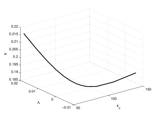
Figure 3: The value of $x_{c}$ for the periodic solutions is shown in dependence on the bulk cosmological constant $\Lambda$ and the brane cosmological constant $\kappa$. Note that $\Lambda$ and $\kappa$ have to be fine-tuned in order to obtain periodic solutions.

4.2.1 Numerical results

In analogy to the $n=2$ case, one could think to construct regular counterparts of the vacuum solutions (6). However, it turns out that all solutions are singular at some finite value of the bulk radial coordinate. We have thus followed a different strategy to construct periodic solutions in $n=3$: we have constructed solutions on an interval $x\in[0:x_{c}]$ that can be continued into periodic solutions on the interval $x\in[0:2x_{c}]$.

We thus impose the following boundary conditions:

$$\phi(0)=0\ ,\ \ \ W(0)=1\ ,\ \ \ M(0)=1\ ,\ \ \ M^{{}^{\prime}}|_{x=0}=0\ ,\ \ \ L(0)=0\ ,\ \ \ L^{{}^{\prime}}|_{x=0}=1\ .$$ (16)

at $x=0$ and

$$M^{{}^{\prime}}|_{x=x_{c}}=0\ ,\ L^{{}^{\prime}}|_{x=x_{c}}=0$$ (17)

at $x=x_{c}$. $\kappa$ and $\Lambda$ can then be fine-tuned in such a way that $W(x=x_{c})=0$ and $\phi(x=x_{c})=0$, i.e. we only find periodic solutions for specific values of the two cosmological constants. Our results are shown in Fig.3, where we show the interdependence of $x_{c}$, $\kappa$ and $\Lambda$ for which periodic solutions exist. In comparison to the $n=2$ case, periodic solutions are also available for a negative bulk cosmological constant. Obviously, $x_{c}$ decreases with the simultaneous increase of the two cosmological constants.

A typical solution for $\gamma=0.2$, $\beta=0.3$ and $x_{c}=50$ is shown in Fig.4. The solutions can then be continued to $x=2x_{c}$ in such a way that

$$M(x_{c}-x) = M(x_{c}+x)\ ,\ L(x_{c}-x)=L(x_{c}+x)\ ,\$$

$$\phi(x_{c}-x) = -\phi(x_{c}+x)\ ,\ W(x_{c}-x)=W(x_{c}+x)\ .$$ (18)

Figure 4: The profiles of the metric functions $M$ and $L$ as well as of the matter field functions $\phi$ and $W$ are shown for a periodic solution with $\gamma=0.2$, $\beta=0.3$ and $x_{c}=50$.

These solutions were coined “mirror” symmetric in [12]. Due to the fact that the Higgs field function $\phi$ has a further zero at $x=x_{c}$, one would expect a domain wall to lie at this point. Indeed, in [12] it was confirmed that close to $x=x_{c}$ the equations resemble those of a kink solution.

Thus, these solutions provide again example of finite brane world models in which a second “brane” naturally appears.

5 Summary

In this paper, we have discussed periodic solutions which appear in brane world model. These solutions appear if an inflating 3-brane resides in a higher dimensional bulk with $n$ extra dimensions. If the bulk contains a positive cosmological constant, but no matter fields, the brane worlds possess a curvature singularity at the origin. If matter fields are included, periodic solutions which are regular at the origin are possible. In the case of two extra dimensions, we have constructed solutions which resemble the periodic vacuum solution outside the string core, but get modified due to the presence of matter fields in the string core such that the solution is regular at the origin. For three extra dimensions, the presence of the matter fields associated to the local monopole in the bulk cannot regularise the solutions in a similar fashion. However, we managed to construct periodic solutions which have additional “branes” appearing at some finite value of the bulk radial coordinate.

These scenarios are interesting since they provide models with a natural finiteness of the extra dimensions in a by observations confirmed natural setting of an inflating brane.

Y.B. thanks the Belgian FNRS for financial support. B.H. was supported by a CNRS grant. We thank the organisers of the NEB XII conference for their hospitality.

References

References

- [1] V. A. Rubakov and M. E. Shaposhnikov, Phys. Lett. B 125 (1983), 136; 125B (1983), 139.
- [2] G. Dvali and M. Shifman, Phys. Lett. B 396 (1997), 64; 407 (1997), 452.
- [3] I. Antoniadis, Phys. Lett. B 246 (1990), 377.
- [4] N. Arkani-Hamed, S. Dimopoulos and G. Davli, Phys. Lett. B429 (1998), 263; I. Antoniadis, N. Arkani-Hamed, S. Dimopoulos and G. Dvali, Phys. Lett. B 436 (1998), 257.
- [5] L. Randall and R. Sundrum, Phys. Rev. Lett. 83 (1999), 3370.
- [6] L. Randall and R. Sundrum, Phys. Rev. Lett. 83 (1999), 4690.
- [7] K. Akama, Pregeometry in Lecture Notes in Physics, 176, Gauge Theory and Gravitation, Proceedings, Nara, 1982, edited by K. Kikkawa, N. Nakanishi and H. Nariai, 267-271 (Springer-Verlag,1983), hep-th/0001113.
- [8] T. Kaluza, Sitzungsber. Preuss. Akad. Wiss. Berlin K1 (1921), 966; O. Klein, Z. Phys. 37 (1926), 895.
- [9] see e.g. J. Polchinski, String Theory, Cambridge University Press (1998).
- [10] P. Breitenlohner, P. Forgacs and D. Maison, Phys. Lett. B 489 (2000) 397.
- [11] Y. Brihaye, T. Delsate and B. Hartmann, Phys. Rev. D 74 (2006) 044015.
- [12] Y. Brihaye and T. Delsate, “Inflating branes inside hyper-spherically symmetric defects”, hep-th/0605039.
- [13] T. Gherghetta, E. Roessl and M. E. Shaposhnikov, Phys. Lett. B 491 (2000), 353; T. Gherghetta and M. E. Shaposhnikov, Phys. Rev. Lett. 85 (2000), 240; M. Giovannini, H. B. Meyer and M. E. Shaposhnikov, Nucl. Phys. B 691 (2001), 615; E. Roessl and M. E. Shaposhnikov, Phys. Rev. D 66 (2002), 084008.
- [14] I. Cho and A. Vilenkin, Phys. Rev. D 68 (2003) 025013; Phys. Rev. D 69 (2004) 045005.
- [15] H. B. Nielsen and P. Olesen, Nucl. Phys. B 61 (1973), 45.
- [16] M. Christensen, A. L. Larsen and Y. Verbin, Phys. Rev. D 60 (1999), 125012; Y. Brihaye and M. Lubo, Phys. Rev. D 62 (2000), 085004.
- [17] G. ’t Hooft, Nucl. Phys. B 79 (1974) 276; A . M. Polyakov, JETP Lett. 20 (1974) 194.