Photoelectron spectra of anionic sodium clusters from time-dependent density-functional theory in real-time

Abstract

We calculate the excitation energies of small neutral sodium clusters in the framework of time-dependent density-functional theory. In the presented calculations, we extract these energies from the power spectra of the dipole and quadrupole signals that result from a real-time and real-space propagation. For comparison with measured photoelectron spectra, we use the ionic configurations of the corresponding single-charged anions. Our calculations clearly improve upon earlier results for photoelectron spectra obtained from static Kohn-Sham eigenvalues.

I Introduction

Since more than one hundred years, photoelectron spectroscopy plays an important role in physics. Einstein’s explanation of the photo-effect, probably the most well-known experiment in the field, was a crucial step in the development of quantum mechanics. Whereas the photo-effect revolutionized the understanding of light, the main aim of modern photoelectron spectroscopy is to understand electronic and ionic structures from solids down to single atoms. Especially in the context of nanoscale materials photoelectron spectroscopy is one of the most important experimental tools since it is almost the only method that provides access to the electronic and ionic structures of these materials. The direct observation of the electronic shell structure in sodium clusters wrigge is just one example for the power of the method. Another application is the determination of the ionic structure of, e.g., clusters. Since the electronic structure, and thus the photoelectron spectrum (PES), depends on the ionic configuration, comparing the measured PES with the results from first-principle calculations allows the identification of the ionic structure. This interplay between theory and experiment has already been used successfully in many cases gantefoer1 ; akolaal ; jenadetach ; kronik ; mosnegna ; gantefoer2 ; jyvasna59 ; agaucupes ; Kost07 .

Clearly, the just mentioned method can only work if reliable calculations for the system of interest can be performed. Since most of the measured systems consist of many electrons, density-functional theory (DFT) is an especially well-suited tool due to its low numerical costs. Unfortunately, evaluating the PES from a Kohn-Sham (KS) DFT calculation is not an easy task since only the highest occupied KS eigenvalue has a rigorous connection to the PES: it is equal to the ionization potential ionizationupot ; almbladh ; PerdLevComm . Thus, it yields the position of the first peak in the PES.

The most common approach to obtain the other peaks in the PES from a DFT calculation is based on the density of states of the occupied KS orbitals. In this approach the KS eigenvalue spectrum of the ‘mother’ system, i.e., the system which still contains the photoelectron, is directly compared to the experimental PES. In many situations the resulting spectra reproduce the experimental ones quite well gantefoer1 ; akolaal ; jenadetach ; kronik ; mosnegna ; gantefoer2 ; jyvasna59 ; agaucupes ; chong ; MWHH1 ; Kost07 .

Another way to extract the information related to the PES from a DFT calculation is via the excitation energies of the ‘daughter’ system, i.e., the system with one electron less. Since time-dependent DFT (TDDFT) RG ; TDDFTRev , in principle, allows to calculate the excitation energies of a system exactly, TDDFT can be used to calculate the positions of the PES peaks accurately. This approach is followed in Ref. C84KA, and Ref. MWHH2, . The basic idea of this approach is also used in Ref. BonKou, , but in combination with configuration-interaction and not TDDFT calculations.

We finally want to mention a third method how the PES can be obtained from a DFT calculation. In this approach, the time-dependent ionization process is simulated in real-time and the kinetic energy spectrum of the outgoing components of the KS Slater determinant are connected to the PES APPG2 .

In Ref. mosnegna, , the PES resulting from Na${}_{5}^{-}$, Na${}_{7}^{-}$, and Na${}_{9}^{-}$ (among others) irradiated by an XeCl excimer laser ($\hbar\omega=4.02$ eV) were measured and compared with the corresponding KS eigenvalue spectra. Although the agreement between the theoretical results and the measured PES was generally reasonable, a systematic discrepancy was found. Namely, the width of the theoretical spectrum, i.e., the difference between the energy of the energetically highest and lowest occupied KS eigenvalue, was too large by about 0.2-0.4 eV. In Ref. mmsk, the reason for this discrepancy was examined. It was shown that technical aspects, e.g., the treatment of the pseudopotential, could not explain the differences. Furthermore, it was demonstrated that using the exchange-only optimized-effective potential (OEP) OEP1 reduced the width of the KS spectrum but not to an extent that would bring the spectrum in agreement with experiment. In addition, it was also shown that using Slater’s transition state concept could also not improve the theoretical results. Thus, the question arises whether a different method to extract the PES from a DFT calculation leads to a better agreement with the experiment. It is the aim of the present manuscript to answer this question by extracting the PES from the excitation energies of the corresponding ‘daughter’ systems.

II Theoretical background

Before discussing the results let us sketch the theoretical background of the presented calculations in more detail.

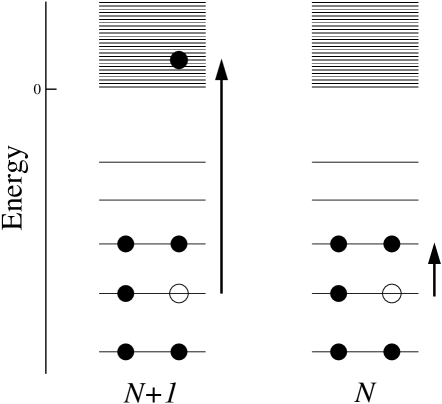
Figure 1: Schematic view of two different approaches to calculate the PES. Left: The process is described as a strong excitation of the $(N+1)$-electron system. Right: The photoelectron has already been detected and the remaining $N$-electron system is left in an excited state. The link between the kinetic energy of the photoelectron and the energy of the excited state of the $N$-electron system is provided by energy conservation.

Fig. 1 schematically shows two approaches how the peak positions in the PES can be calculated. On the left hand side, the process is described as an excitation process from the ground state to an energetically high-lying state with continuum contributions. Since KS eigenvalue differences are zeroth-order approximations to excitation energies AGExcitKS ; Gonze , the KS DOS of the $(N+1)$-electron system can be used to obtain an approximate PES. In addition to this argument, Chong et al. chong have given well founded arguments that KS eigenvalues can be interpreted as approximations to relaxed vertical ionization potentials.

On the right hand side of Fig. 1, the situation after the photoelectron has been detected is considered. In this case, the remaining system is left in an energetically low-lying excited state of the $N$-electron system. To connect the excitation energies of this system to the PES, energy conservation is used. Before the photon is absorbed the total energy is given by $E_{0}^{(N+1)}\,+\,\hbar\omega$, where $E_{0}^{(N+1)}$ is the ground-state energy of the ‘mother’ system containing $N+1$ electrons and $\hbar\omega$ is the photon energy. After the detection of the photoelectron the total energy is given by the kinetic energy of the photoelectron $E_{\mathrm{kin}}$ and the energy of the remaining ‘daughter’ system. Since the total energy is conserved, it follows that

$$E_{\mathrm{bind},j}=E_{\mathrm{kin}}-\hbar\omega=E_{0}^{(N+1)}-E_{0}^{(N)}-\Delta E_{j}^{(N)}$$ (1)

must hold. Here, $E_{0}^{(N)}$ is the ground-state energy of the ‘daughter’ system and $\Delta E_{j}^{(N)}$ are its excitation energies Remark1 . For the first peak in the PES the kinetic energy of the photoelectron is maximal. In this case, the ‘daughter’ system is in its ground-state, i.e., $\Delta E_{j}^{(N)}$ is zero and the peak position is at $E_{0}^{(N+1)}-E_{0}^{(N)}$.

To obtain the excitation energies from time-dependent DFT the full linear density-response function of the interacting system can be used. This function provides access to the excitation energies of the system since it has poles at these energies. The crucial observation now is that the interacting linear density-response function can be expressed in terms of the KS response function and the exchange-correlation (xc) kernel TDDFTExcit ; Casida ; TDDFTRev . Nowadays, most applications use the matrix equation of Casida Casida to obtain these excitation energies.

Alternatively, the excitation energies can be extracted from a spectral analysis of the time-dependent density coming from a real-time propagation Bertsch ; PG ; Octop . In this approach, the xc kernel is not needed, but instead, the time-dependent KS equations are solved without explicit linearization. To illustrate this approach, imagine we have created a time-dependent density $n({\bf r},t)$ of an interacting system by, e.g., a laser excitation. Assuming that the system is confined by the same time-independent potential before and after the laser pulse we can write the excited density in terms of the eigenstates $|\psi_{j}\rangle$ of the interacting system in the time-independent potential. It reads

$$n({\bf r},t) = \langle\psi(t)|\hat{n}|\psi(t)\rangle$$ (2)

$$= \sum_{j,k}c_{j}^{*}c_{k}\langle\psi_{j}|\hat{n}|\psi_{k}\rangle\exp(-i(E_{k}-E_{j})t/\hbar)$$

where $E_{j}$ is the eigenvalue corresponding to $|\psi_{j}\rangle$ and $\hat{n}$ is the density operator. Assuming that the time-dependent state $|\psi(t)\rangle$ is dominated by the ground state, i.e., $c_{0}\gg c_{j}$ we can write

$$n({\bf r},t) \approx |c_{0}|^{2}n_{0}({\bf r})\ +$$ (3)

$$\sum_{j} c_{0}^{*}c_{j}\langle\psi_{0}|\hat{n}|\psi_{j}\rangle\exp(-i(E_{j}-E_{0})t/\hbar)+c.c.\ ~{}~{}~{}$$

Here, $n_{0}({\bf r})$ is the ground-state density of the system. If we now calculate the Fourier transform of $n({\bf r},t)$ we will get peaks at the exact excitation energies of the system. Since time-dependent DFT in principle provides us with the exact time-dependent density, this is an easy method to obtain the excitation energies of the interacting system from a time-dependent DFT calculation.

In a practical calculation, two problems must be solved to get the excitation energies from this scheme. First, one has to create a time-dependent density which is dominated by the ground-state density and, in addition, contains the excited states of interest. The second problem is how to extract the excitation energies from the time-dependent density in practice. Since the density in every space point at all times cannot be stored, a full Fourier transform of Eq. (3) giving $n({\bf r},\omega)$ is not possible. To overcome this problem several possibilities exist. One is to evaluate $n({\bf r},\omega)$ only for some points in space SKPGDensPlas , e.g., in the center of the cluster. A different method is to Fourier transform certain moments of the density distribution. Typically, the dipole moment is used for this purpose Bertsch ; PG . Obviously, some excitations are filtered out by this procedure because the Fourier spectrum of the dipole moment only shows excitation energies of states which can be coupled to the ground state via the dipole operator. Non-dipole active excitations can be taken into account by recording higher moments. In the following we will use the time-dependent dipole and quadrupole moments obtained from a real-time propagation to obtain excitation energies for the systems of interest.

III Technical aspects

For the ionic ground-state configurations of the ‘mother’ systems we used optimized structures obtained with the PARSEC Parsec program package. The generalized-gradient approximation of Perdew et al. (PBE) PBE was employed for the geometry optimization. The ionic cores were treated consistently with norm conserving non-local pseudopotentials TroullierM .

The time-dependent KS equations were solved on a real-space grid in real time. For this we implemented the necessary algorithms into a modified version of the PARSEC code. In detail, we implemented a fourth-order Taylor approximation to the propagator in combination with a higher-order finite-difference formula for the kinetic part of the KS Hamiltonian. For the calculations, we used a time step of 0.003 fs and the total propagation time was 75 fs. The ionic cores were again described by norm conserving non-local pseudopotentials. Furthermore, the ionic structures were fixed during the propagation. The grid spacing was 0.7 $a_{0}$ and the grid radius varied between 20 and 23 $a_{0}$ depending on the system. The time-dependent density was created by applying a boost $\exp(i\,\mathbf{r}\cdot\mathbf{p}_{\mathrm{boost}}/\hbar)$ to the ground-state KS orbitals. The total excitation energy of the system was $E_{\mathrm{excit}}=1.0\times 10^{-5}$ eV, i.e., a boost strength $|p_{\mathrm{boost}}|=\sqrt{2m_{e}E_{\mathrm{excit}}/N}$ was applied to each KS orbital (with $m_{e}$ being the electron mass and $N$ the number of electrons). In addition, the calculations were repeated with a boost strength reduced by a factor of $1.0\times 10^{-2}$. Using these two small boost strengths allowed us to check whether the created time-dependent density was dominated by the ground-state density (see below).

Instead of applying the same boost vector $\mathbf{p}_{\mathrm{boost}}$ to all KS orbitals, and thus creating a coherent velocity field, we varied the boost direction for different KS orbitals. This is necessary since applying the same boost direction to all KS orbitals corresponds to first order in $\mathbf{p}_{\mathrm{boost}}$ to a dipole excitation of the system, i.e., from the resulting time-dependent density it is only possible to retrieve the excitation energies of ‘dipole-active’ states. By applying different boost directions to different KS orbitals we modeled a general excitation mechanism creating a time-dependent density containing excited states with different symmetry properties. In detail, we randomly chose a boost direction (no symmetry axis of the considered cluster) for the first orbital and then chose our coordinate system such that this direction was the first diagonal (for the remaining rotational degree of freedom a random angle was chosen). After this we boosted the second orbital in the opposite direction of the first boost. The third orbital was then boosted in the direction of the second diagonal of the chosen coordinate system, the forth again in the opposite direction and so on. For Na₉, the ninth orbital was boosted again in the same direction as the first orbital. Since the only purpose of this procedure was to create a time-dependent density without any particular symmetries, we do not consider the relative orientation of the cluster with respect to the boost directions to be of special importance.

Finally, we used the time-dependent local-density approximation (TDLDA) ALDA for the xc potential for the propagation. Since the linear response of the homogeneous electron gas is the same in this approximation and in the PBE functional, the differences in the resulting excitation energies can be expected to be small in the low-energy regime. Unfortunately, the exact-exchange orbital functional cannot be used for comparative calculations since it requires a solution of the time-dependent optimized-effective potential equation TDOEP and no method for this exists in real-time at the moment MMSKTDOEP .

IV Results and discussion

IV.1 Results for Na${}_{3}^{-}$

Fig. 2 shows the dipole power spectra of Na₃ resulting from two boost strengths differing by a factor of $10^{2}$. The dipole power spectrum is given by

$$D(\omega)\ :=\ \sum_{j=1}^{3}|d_{j}(\omega)|^{2}$$ (4)

with $d_{j}(\omega)$ being the Fourier transform of the dipole moment

$$d_{j}(t)\ =\ \int x_{j}\,n({\bf r},t)\ d^{3}r$$ (5)

where $x_{1}$ corresponds to the Cartesian coordinate $x$, $x_{2}$ to $y$, and $x_{3}$ to $z$.

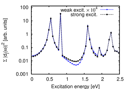
Figure 2: (Color online) Dipole power spectrum of Na₃ resulting from an incoherent boost excitation. The result obtained from a total excitation of $1\times 10^{-5}$ eV is labeled ‘strong excit.’ whereas the label ‘weak excit.’ corresponds to a boost reduced by a factor of $1\times 10^{-2}$. Clearly, the dipole power spectrum scales quadratically with the boost strength indicating that the peak positions correspond to excitation energies between the ground state and excited states.

For small momentum boosts first-order perturbation theory predicts a linear dependence of the expansion coefficients $c_{j}$ in Eq. (2) on the boost strength. As a consequence, reducing the boost strength by a factor of $c$ suppresses peaks corresponding to energy differences between two excited eigenstates by a factor of $c^{4}$ in the power spectrum. Since peaks corresponding to transitions between the ground state and an excited eigenstate are only suppressed by a factor of $c^{2}$, changing the boost strength allows one to distinguish between these two kinds of excitations. As one can see in Fig. 2, the results for the two boost strengths are almost identical except for the predicted factor of $10^{4}$. Thus, we conclude that all the peak positions in the dipole power spectrum of Fig. 2 correspond to energy differences between the ground state energy and the energy eigenvalues of the excited eigenstates.

The situation is different for the power spectrum resulting from the quadrupole moments. In Fig. 3 we plot

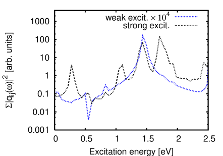
Figure 3: (Color online) Sum of the absolute square of the Fourier-transformed components of the quadrupole tensor resulting from the same excitations as in Fig. 2. In contrast to the dipole power spectrum some peaks vanish with reduced boost strength indicating that they correspond to energy differences between excited states.

$$Q(\omega):=\sum_{\stackrel{{\scriptstyle i=1}}{{j\geq i}}}^{3}|q_{ij}(\omega)|^{2}$$ (6)

for the same two excitation boosts. In this equation, $q_{ij}(\omega)$ is the Fourier transform of the quadrupole moment

$$q_{ij}(t) = \int n({\bf r},t)\,(3x_{i}x_{j}\,-\,r^{2}\delta_{ij})\ d^{3}r\ ,$$ (7)

$$r^{2} = \sum_{i=1}^{3}x_{i}^{2}\ ,$$

and the sum only runs over the independent components of the quadrupole tensor. Clearly, the quadrupole spectra for the different excitation strengths differ considerably. For instance, the three large peaks at around $0.3$, $1.1$, and $1.7$ eV vanish almost completely. Thus, we conclude that they belong to transition energies between different excited states. Indeed, one can see that these energies are exactly equal to the energy differences between the first excited state and the other excited states from the dipole spectrum.

The reason why there are no peaks at these energies in the dipole spectrum can easily be understood if one takes the geometry of Na₃ into account. Since Na₃ has a linear ionic configuration, the ground state has even parity. Thus, the dipole spectrum only shows excited states with odd parity. Since two states with odd parity cannot be coupled by the dipole operator, transitions between these states do not show up in the dipole spectrum.

After the identification of the true excitation energies we can now compare the results with the measured PES. In Fig. 4 the excitation energies of Na₃, the KS DOS of Na${}_{3}^{-}$ and the measured PES (of Na${}_{3}^{-}$) are plotted. The positions of the occupied KS eigenvalues are indicated by arrows, long bars indicate excitation energies from the dipole spectrum and shorter bars excitation energies from the quadrupole moments. In addition, excitation energies leading to peaks below the strongest bound experimental peak are reduced in their overall height. For better comparison, the KS DOS and the excitation spectrum are both rigidly shifted in such a way that the most weakly bound peak coincides with the experimental one.

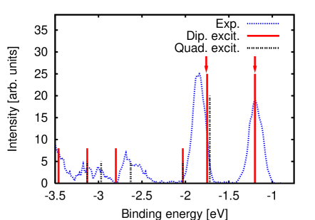
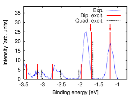
Figure 4: (Color online) Measured PES of Na${}_{3}^{-}$ (‘Exp.’) and theoretical PES obtained from the excitation energies of Na₃. Excitation energies from the dipole spectrum are labeled ‘Dip. excit.’ whereas ‘Quad. excit.’ labels excitation energies deduced from the quadrupole moments. Arrows indicate the result obtained from the KS DOS. Upper part: results obtained from the ionic ground-state configuration at zero temperature. Lower part: results obtained from an ionic configuration with a larger bond length to simulate a higher temperature. For most peaks the agreement with the experimental PES is clearly improved.

As the upper part of Fig. 4 shows the peak positions that one obtains from the KS DOS are close to the experimental peak positions. Unlike in the case of larger Na clusters, the width is slightly smaller than the energy difference between the two large experimental peaks but it is still reasonable. However, since there are only two occupied KS orbitals in Na${}_{3}^{-}$ the KS DOS picture fails completely to describe the higher lying peaks in the measured spectrum.

As one expects from Eq. (1) the PES obtained from the excitation energies shows a much richer structure than the KS DOS. One striking feature for instance is the second excitation around $-2.0$ eV. It seems that the energy difference between this peak and the one at $-1.7$ eV is too large in the calculation and that they are merged to one peak in the experimental PES. However, in general, the dynamically calculated excitation energies and the energies obtained from the experimental PES are close to each other even for the stronger bound peaks. To see if the remaining discrepancy can be further reduced by taking temperature effects into account we have repeated our calculations with a larger bond length. Due to the net negative charge of the cluster one can expect that other geometry changes, e.g., bending, only play a minor role in the case of Na${}_{3}^{-}$. We have used a new bond length of approx. $6.8$ instead of $6.5$ $a_{0}$. This new value for the bond length $l$ of the cluster has been obtained from an estimate for the thermal expansion at $T=300$ K. It is based on the formula $\beta=\frac{1}{l}\frac{\partial l}{\partial T}$ for the linear thermal expansion coefficient $\beta$ which we have roughly estimated by $\beta\approx 2\,\beta_{\mathrm{bulk}}$ (see Ref. SKTherm, ), where $\beta_{\mathrm{bulk}}$ is the bulk value for crystalline sodium at room temperature.

The result can be seen in the lower part of Fig. 4. For most peaks one can observe a small shift towards lower absolute binding energies. Except for the peak at $-1.7$ eV the agreement between the experimental and theoretical spectrum is slightly improved by the increased bond length. Especially the broader peak at around $-2.6$ eV is nicely reproduced in this case. All in all, both calculations show that for Na${}_{3}^{-}$ the main advantage of the ‘excitation picture’ is the reproduction of the deeper bound structures in the PES.

IV.2 Results for Na${}_{5}^{-}$

Fig. 5 shows the experimental PES of Na${}_{5}^{-}$, the KS DOS, and the PES obtained from the excitation energies of Na₅. The labeling is the same as in the corresponding previous figures. As for Na${}_{3}^{-}$, the KS DOS is in acceptable agreement with the first large peaks, although the strongest bound large peak has a too negative binding energy in the KS DOS. As one can see these peaks are also well described by the excitation energies of the ‘daughter’ system with the additional advantage that the last peak at $-2.2$ eV is better reproduced. In this approach it consists of four close-lying excitations.

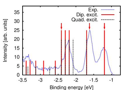
Figure 5: (Color online) Same as in Fig. 4 but for Na${}_{5}^{-}$. Although both, the KS DOS and the PES from the excitation energies, describe the measured PES acceptable the large peak at $-2.2$ eV is much better reproduced by the excitation energies from the ‘daughter’ system. The experimental data is taken from Ref. mosnegna, .

Beyond the peak at $-2.2$ eV the comparison with the experimental measurement is difficult since no clear peak structures can be observed. Perhaps the accumulation of excited states around $-3.3$ eV can be associated with the measured peak in this region, but for the reasons given below, one has to be very cautious in making comparisons in this part of the spectrum.

As one can see from the results for Na${}_{7}^{-}$ and Na${}_{9}^{-}$ discussed below the problem of comparing the deeper lying part of the measured PES with calculated excitation energies is not specific to Na${}_{5}^{-}$. In general, the density of excited states grows with the excitation energy, i.e., more and more states appear in the theoretical calculation. On the other hand, from the point of view of first-order perturbation theory the PES depends not only on the positions of the excited states but also on the matrix element of the perturbing operator $\hat{D}$ between the initial and the final state. Taking the ground state of the ‘mother’ system for the initial state and a product state consisting of one photoelectron with momentum $\mathbf{k}$ for the final state one obtains matrix elements of the form $\langle\mathbf{k},\,\psi_{j}^{(N)}|\ \hat{D}\ |\psi_{0}^{(N+1)}\rangle$. It is intuitively clear that these matrix elements are much larger for low-lying states than for energetically high-lying ones which in an independent-particle picture would correspond to removing one particle and exciting a second one above the Fermi level. Especially, in the case of truly independent particles this process cannot happen if the perturbing operator is a one-particle operator like the dipole operator. Thus, many energetically high-lying eigenstates of the ‘daughter’ system are hardly or even not at all excited in the experiment. Since the mentioned matrix elements depend on the interacting many-particle wavefunctions, calculating these exactly is close to being impossible. Especially, retrieving these matrix elements from a TDDFT propagation of the ‘daughter’ system is not trivial because the propagation only provides information about matrix elements between excited states and the $N$-particle ground state and not the $(N+1)$-particle ground state.

However, as the presented calculations show, the matrix elements do not play a very important role in the part of the spectrum that we are mainly interested in. Nevertheless, the calculations also clearly indicate that one has to consider them if the deeper lying parts of the spectrum are of interest. A possible method how this can be done in a TDDFT calculation can be found at the end of Sec. V.

IV.3 Results for Na${}_{7}^{-}$

The results for Na${}_{7}^{-}$ are shown in Fig. 6. As said previously, in the region below $-2.5$ eV, it is difficult to compare theory and experiment due to the great number of close lying transitions. As in Na${}_{5}^{-}$, the KS DOS describes the strongest bound large peak worst. In this case it is already off by $0.4$ eV. In contrast, the peak position obtained from the TDLDA excitation energies is considerably closer to the experimental peak. It is only off by $0.1$ eV. Thus, the overestimation of the spectrum’s width by the KS DOS mosnegna ; mmsk is not observed in the result obtained from the TDLDA calculation. The remaining difference of $0.1$ eV between the width of the theoretical and the experimental spectrum can be easily caused by technical aspects like the employed pseudopotential and xc potential mmsk . In addition, thermal effects like bond elongation and structural isomerization can shift the obtained width by $0.1$ eV SKTherm ; mosnegna ; moshhulPRL . Considering that the experimental PES were obtained from clusters with a temperature of around 250-300 K, the difference between the theoretical result at zero temperature and the experimental result is hardly surprising. At these temperatures the larger anionic sodium clusters behave liquidlike mosnegna . Consequently, many different ionic configurations are present in the experiment and show up in the measured PES.

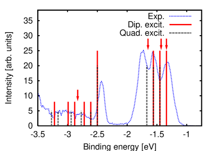
Figure 6: (Color online) Same as in Fig. 4 but for Na${}_{7}^{-}$. Especially, the peak at $-2.4$ eV is much more accurately described by the excitation energies than by the KS DOS. In the weakly bound region thermal effects play an significant role in the case of Na${}_{7}^{-}$. This explains the rather poor agreement between the theoretical values calculated at zero temperature and the measured curve between $-1.3$ and $-1.7$ eV. The experimental data is taken from Ref. mosnegna, .

This aspect must also been kept in mind if the theoretical and experimental results are compared in the region between $-1.3$ and $-1.7$ eV. In this region both the zero temperature KS DOS result and the zero temperature result from the excitation energies do not describe the measured PES very accurately. Especially, the excitation peak at $-1.45$ eV does not fit very well. However, from Ref. mosnegna, it is known that the agreement between the experimental and the KS DOS result in this energy region is significantly improved if different ionic structures are taken into account via Born-Oppenheimer Langevin molecular-dynamics BarnLand . Therefore, one can expect that the agreement between the experimental and the TDLDA result is also improved if different ionic structures are taken into account. Due to the more complicated structures and the growing number of isomers the inclusion of the temperature influence on the ionic structures of larger clusters is much more involved than in the case of Na${}_{3}^{-}$. Additionally, combining Born-Oppenheimer Langevin molecular-dynamics with the calculation of excitation energies is substantially more expensive than combining such a molecular dynamics scheme with a KS DOS calculation. Thus, including thermal effects in the present study is beyond the scope of the present work and is a future project.

IV.4 Results for Na${}_{9}^{-}$

Finally, the theoretical results for Na${}_{9}^{-}$ are compared in Fig. 7 with the measured PES. This cluster is the first one which has a clear peak in the range between the highest and lowest occupied KS eigenvalue which is completely absent in the KS DOS, i.e., the experimental PES shows six clear peaks whereas the KS DOS consists of only five peaks: the peak around $-2.4$ eV is completely missing in the KS DOS. In addition, the strongest bound peak in the KS DOS is off by $0.5$ eV. In other words, the KS DOS result is inaccurate to the extent of being useless below $-2.2$ eV. As for Na${}_{7}^{-}$, the splitting of the large peak around $-1.8$ eV is reproduced if different ionic structures are used mosnegna .

In contrast to the KS DOS result, the PES obtained from the excitation energies is close to the measured curve over the whole range. Below the lowest lying peak at $-2.7$ eV the comparison is again difficult without knowing the matrix elements mentioned above. For the two peaks at $-2.7$ and $-2.4$ eV the theoretical values are off by $0.1$ eV. Especially since Na${}_{9}^{-}$, in contrast to Na${}_{7}^{-}$, is not a closed-shell cluster, one can expect that such energy differences can be easily caused by ionic structure modifications induced by finite temperatures. As expected from Ref. mosnegna, , the splitting of the peak at $-1.8$ eV is also not reproduced by the zero temperature TDLDA calculation. All in all, the experimental result in the weaker bound part of the spectrum is described equally well by the KS DOS and the excitation energies of the ‘daughter’ system. However, in the stronger bound part the time-dependent calculation yields a much more realistic description of the PES than the KS DOS. Since this emerges as a general observation for all systems studied in this manuscript, we discuss it on general grounds in the following section.

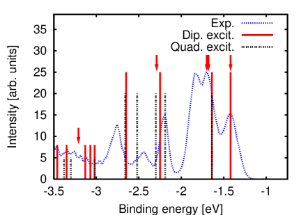
Figure 7: (Color online) Same as in Fig. 4 but for Na${}_{9}^{-}$. As in Na${}_{7}^{-}$, especially the stronger bound part of the spectrum is described more accurately by the calculated excitation energies than by the KS DOS. The experimental data is taken from Ref. mosnegna, .

V Summary and Conclusion

Using TDDFT we have calculated the excitation energies of small neutral sodium clusters. The energies of the excited states were retrieved from the dipole and quadrupole moments of the time-dependent density via spectral analysis. The time-dependent density was created by an incoherent boost of all KS ground-state orbitals and then propagated in real-space and real-time. To discriminate between true excited state energies and energies corresponding to energy differences between excited states we did two calculations for all systems using different excitation energies. For comparison with measured PES of the anionic clusters the excitation energies were calculated in the ionic configuration of the anions.

In general, the PES for all clusters studied in this manuscript can be divided into three parts. The first part consists of large, ‘weakly’ bound peaks, the second of large, ‘strongly’ bound peaks, and finally a ‘less structured’ region below the lowest large experimental peak. Except for Na${}_{3}^{-}$ no comparisons between our theoretical and the experimental results can be made in the third region. As discussed in Subsection IV.2 the main reason for this is the missing access to the transition matrix elements between the ground and the excited states. Since the number of excited states can grow very rapidly, one can expect that the omission of the transition matrix elements can cause severe problems if more complex systems are examined. A possible way to overcome this problem is by including the information of the matrix elements in the initial density, i.e., by creating an initial density that only includes the states which are really excited in the ionization process. Work in this direction is under way.

In the middle part of the spectrum the results obtained from the TDLDA excitation energies are clearly superior to the results from the KS DOS. Especially, the position of the strongest bound large peak is much better reproduced by the TDLDA calculation than by the KS DOS. Thus, using the TDLDA cures the main problem that plagues theoretical results obtained from the KS DOS for sodium clusters, namely the prediction of a significantly too large width of the spectrum. In addition, the PES from the TDLDA excitations can describe an experimental peak in the PES of Na${}_{9}^{-}$ which is completely missing in the KS DOS. The remaining differences between the experimental and our theoretical results are all small enough to be explainable by technical details or the finite temperature (250-300 K) of the ionic structures in the experiment. In particular the finite temperature can be expected to be responsible for the difference since the considered clusters behave liquidlike at this temperature and thus, the measured PES result from many different ionic structures / isomers which differ from the theoretical zero temperature ground-state structures used for the calculations.

Finally, in the most weakly bound part of the spectrum we find that the TDLDA result and the one from the KS DOS are very similar. Since the KS DOS at finite temperature is in very good agreement with the experimental result mosnegna , it is extremely likely that also the TDLDA excitation energies calculated from higher temperature ionic structures will describe the experimental PES very well in this region.

Generally, our findings are in line with earlier results PerdNor ; chong which report a worse agreement between the KS DOS results and the experimental values for stronger bound levels. In addition, our results clearly show that the agreement between the theoretical and the experimental spectrum is considerably improved for small sodium clusters if the PES is extracted from the true excitation energies of the ‘daughter’ system and not the KS DOS. This shows the importance of taking effects beyond the independent-particle picture into account in the interpretation of photoelectron spectra.

- (1) G. Wrigge, M. Astruc Hoffmann, and B. v. Issendorff, Phys. Rev. A 65, 063201 (2002).
- (2) H. Kietzmann, J. Morenzin, P. S. Bechthold, G. Ganteför, W. Eberhardt, D. S. Yang, P. A. Hackett, R. Fournier, T. Pang, and C. F. Chen, Phys. Rev. Lett. 77, 4528 (1996).
- (3) J. Akola, M. Manninen, H. Häkkinen, U. Landman, X. Li, and L.-S. Wang, Phys. Rev. B 62, 13216 (2000).
- (4) S. N. Khanna, M. Beltran, P. Jena, Phys. Rev. B 64 235419 (2001).
- (5) L. Kronik, R. Fromherz, E. Ko, G. Ganteför, and J. R. Chelikowsky, Nat. Mater. 1, 49 (2002).
- (6) M. Moseler, B. Huber, H. Häkkinen, U. Landman, G. Wrigge, M. A. Hoffmann, and B. v. Issendorff, Phys. Rev. B 68, 165413 (2003).
- (7) N. Bertram, Y. D. Kim, G. Ganteför, Q. Sun, P. Jena, J. Tamuliene, and G. Seifert, Chem. Phys. Lett. 396, 341 (2004).
- (8) K. Manninen, H. Hakkinen, and M. Manninen, Phys. Rev. A 70, 023203 (2004).
- (9) H. Häkkinen, M. Moseler, O. Kostko, N. Morgner, M. A. Hoffmann, and B. v. Issendorff, Phys. Rev. Lett. 93, 093401 (2004).
- (10) O. Kostko, B. Huber, M. Moseler, and B. von Issendorff, Phys. Rev. Lett. 98, 043401 (2007).
- (11) M. Levy, J. P. Perdew, and V. Sahni, Phys. Rev. A 30, 2745 (1984).
- (12) C.-O. Almbladh and U. von Barth, Phys. Rev. B 31, 3231 (1985).
- (13) J. P. Perdew and M. Levy, Phys. Rev. B 56, 16021 (1997).
- (14) D. P. Chong, O. V. Gritsenko, and E. J. Baerends, J. Chem. Phys. 116, 1760 (2002).
- (15) M. Walter and H. Häkkinen, Eur. Phys. J. D 33, 393 (2005).
- (16) E. Runge and E. K. U. Gross, Phys. Rev. Lett. 52, 997 (1984).
- (17) E. K. U. Gross, J. F. Dobson, and M. Petersilka, in Density Functional Theory, edited by R. F. Nalewajski, Topics in Current Chemistry, Vol. 181, (Springer, Berlin 1996).
- (18) O. T. Ehrler, J. M. Weber, F. Furche, and M. M. Kappes, Phys. Rev. Lett. 91, 113006 (2003).
- (19) M. Walter and H. Häkkinen, to be published.
- (20) V. Bonačić-Koutecký, P. Fantucci, and J. Koutecký, J. Chem. Phys. 91, 3794 (1989).
- (21) A. Pohl, P.-G. Reinhard, and E. Suraud, Phys. Rev. Lett. 84, 5090 (2000).
- (22) M. Mundt, S. Kümmel, B. Huber, and M. Moseler, Phys. Rev. B 73, 205407 (2006).
- (23) R. T. Sharp and G. K. Horton, Phys. Rev. 90, 317 (1953).
- (24) A. Görling, Phys. Rev. A 54, 3912 (1996).
- (25) C. Filippi, C. J. Umrigar, and X. Gonze, J. Chem. Phys. 107, 9994 (1997).
- (26) M. Petersilka, U. J. Gossmann, and E. K. U. Gross, Phys. Rev. Lett. 76, 1212 (1996).
- (27) M. E. Casida, in Recent Developments and Applications in Modern Density-Functional Theory, edited by J. M. Seminario, (Elsevier, Amsterdam, 1996).
- (28) K. Yabana and G. F. Bertsch, Phys. Rev. B 54, 4484 (1996).
- (29) F. Calvayrac, P.-G. Reinhard, E. Suraud, and C. A. Ullrich, Phys. Rep. 337, 493 (2000).
- (30) M. A. L. Marques, A. Castro, and A. Rubio, J. Chem. Phys. 115, 3006 (2001).
- (31) S. Kümmel, K. Andrae, and P.-G. Reinhard, Appl. Phys. B 73, 293 (2001).
- (32) Ionic relaxation processes are neglected here, i.e., we assume that the ions do not move during the time interval between the photon absorption and the photoelectron detection. As a consequence, the excitation energies of the ‘daughter’ system are calculated in the ionic configuration of the ‘mother’ system.
- (33) L. Kronik, A. Makmal, M. L. Tiago, M. M. G. Alemany, M. Jain, X. Huang, Y. Saad, and J. R. Chelikowsky, Phys. Stat. Sol. (b) 243, 1063 (2006).
- (34) J. P. Perdew, K. Burke, and M. Ernzerhof, Phys. Rev. Lett. 77, 3865 (1996).
- (35) N. Troullier and J. L. Martins, Phys. Rev. B 43, 1993 (1991).
- (36) T. Ando, Z. Phys. B 26, 263 (1977).
- (37) C. A. Ullrich, U. J. Gossmann, and E. K. U. Gross, Ber. Bunsenges. Phys. Chem. 99, 488 (1995); Phys. Rev. Lett. 74, 872 (1995).
- (38) M. Mundt and S. Kümmel, Phys. Rev. A 74, 022511 (2006).
- (39) S. Kümmel, J. Akola, and M. Manninen, Phys. Rev. Lett. 84, 3827 (2000).
- (40) M. Moseler, H. Häkkinen, and U. Landman, Phys. Rev. Lett. 87, 053401 (2001).
- (41) R. Barnett and U. Landman, Phys. Rev. B 48, 2081 (1993).
- (42) J. P. Perdew and M. R. Norman, Phys. Rev. B 26, 5445 (1982).