Quantum state tomography using a single apparatus

Abstract

The density matrix of a two-level system (spin, atom) is usually determined by measuring the three non-commuting components of the Pauli vector. This density matrix can also be obtained via the measurement data of two commuting variables, using a single apparatus. This is done by coupling the two-level system to a mode of radiation field, where the atom-field interaction is described with the Jaynes–Cummings model. The mode starts its evolution from a known coherent state. The unknown initial state of the atom is found by measuring two commuting observables: the population difference of the atom and the photon number of the field. We discuss the advantages of this setup and its possible applications.

1 Introduction

Determining the unknown state of a quantum system is the basic inverse problem of quantum mechanics. Given the state, one can calculate the expectation value of any observable of the system deMuynck . However, the inverse problem of determining the state by performing different measurements is non-trivial. This problem was discussed by Pauli Pauli in 1933. His question was whether one can reconstruct the unknown wave-function of an ensemble of identical spinless particles via the corresponding position and momentum probability densities. The interest to the state determination problem grew considerably since then, and now this is a well-recognized subject Kemble .

The notion of state refers to an ensemble of identically prepared systems and is represented by a Hermitian operator with non-negative eigenvalues that sum to one (density matrix) deMuynck . Thus the $N\times N$ density matrix of an ensemble of $N$-level systems is specified by $N^{2}-1$ independent real parameters. Since any observable $\hat{\mathcal{O}}$ of the system generates at most $N-1$ independent probabilities, at least $(N^{2}-1)/(N-1)=N+1$ measurements of non-commuting observables are needed to obtain the unknown state brut .

Procedures of reconstructing the quantum state from measurements are known as quantum state tomography. Recently they found applications in quantum information processing Nielson . For example, in quantum cryptography one needs a complete specification of the qubit state Pasqui . For the simplest example of a spin-$\frac{1}{2}$ system the state is described by a $2\times 2$ matrix. According to the above argument, one has to perform $3$ incompatible measurements for the unknown state determination, e.g., measuring the spin components along the x-, y- and z- axes via the Stern-Gerlach setup. However, during the measuremental procedure of each component one looses the information about the two other components, since the spin operators in different directions do not commute. Thus, to determine the state of a spin-$\frac{1}{2}$ system, one needs to use repeatedly three Stern–Gerlach measurements performed along orthogonal directions.

However, the state can be characterized indirectly via a single set of measurements performed simultaneously on the system of interest and an auxiliary system (assistant), which starts its evolution from a known state D'Ariano ; PRL ; peng . This can be done by letting them interact for a specific time and measuring commuting observables of the overall system (system+assistant). In particular, it has been shown that one can determine the unknown state of a spin-$\frac{1}{2}$ system with a single apparatus by using another spin-$\frac{1}{2}$ assistant PRL . The idea was recently implemented by Peng et. al. peng who used pulses to induce the proper dynamics of the interaction between a spin-$\frac{1}{2}$ system and its assistant. They verified the initial state of the system obtained from this procedure with the results of the direct measurement of the three components of the spin vector of the system.

Our present purpose is to determine the unknown density matrix of an ensemble of two-level systems (atom or spin) via interaction with a single mode of the electromagnetic field. The atom-field interaction is studied within the Jaynes–Cummings model Jaynes . We show that the unknown state of the spin can be completely characterized by measuring two commuting variables: the population difference of the atoms $\hat{\sigma}_{z}$ and the photon number of the field $\hat{a}^{\dagger}\hat{a}$. This measurement supplies three averages: $\langle\sigma_{z}\rangle$, $\langle a^{\dagger}a\rangle$ and $\langle\sigma_{z}\,a^{\dagger}a\rangle$, which will be linearly related to the elements of the initial density matrix of the ensemble of the two-level atoms. (Note that since $\hat{\sigma}_{z}$ and $\hat{a}^{\dagger}\hat{a}$ commute, $\langle\sigma_{z}\,a^{\dagger}a\rangle$ is recovered from the measurement data of $\sigma_{z}$ and $a^{\dagger}a$ via the number of coincidences.)

In section 2 we will give a brief introduction on the Jaynes–Cummings model and its properties. In section 3 the model is used to determine the state of the two-level system. Section 3..1 discusses imperfection of the proposed scheme due to the noise in selecting the measurement time. In section 4 we discuss how to reconstruct the unknown density matrix approximately given an incomplete measurement data. The solution of this task amounts to a direct application of the classical Maximum Likelihood setup, because our scheme operates with the measurement of commuting observables. We conclude in section 5.

2 The Jaynes–Cummings Model

The Jaynes–Cummings model (JCM) Jaynes has a special place in quantum optics and atomic physics Stenholm ; Shore ; Raimond . This model describes the interaction of a two-level atom with a single mode of electromagnetic field, and it was employed by Jaynes and Cummings for studying the quantum features of spontaneous emission. Later on, the model generated several non-trivial theoretical predictions—such as collapes and revivals of the atomic population that are related to the discreteness of photons Cummings ; Eberly —which were successfully tested in experiments Haroche . In particular, the model explains experimental results on one-atom masers Haroche , and on the passage of (Rydberg) atoms through cavities Rempe2 ; Walther1 ; Osnaghi ; Meunier . The JCM is also used for describing quantum correlation and formation of macroscopic quantum states. It was recently employed in quantum information theory Ellin ; JCinfo . More recently, the JCM found applications in semiconductors semiconductor and in Josephson junctions josephson .

The JCM is in fact a family of models, since the original model of Jaynes and Cummings was generalized several times for a more adequate description of the atom-field interaction (e.g., multi-mode fields, multi-level atoms, damping) Kundu ; Hussin ; Rodri . We shall however study the simplest original realization of the JCM that involves a two-level atom interacting with a single mode of electromagnetic field. In particular, we neglect the effects of noise and dissipation. This situation has direct experimental realizations Haroche ; Garching ; Har2 . For instance with the superconducting microcavities one can achieve $\sim 0.1$s for the average lifetime of the cavity photon, much larger than the typical field-atom interaction time $\sim 100-500\mu s$ Rempe2 ; Meunier .

The quantized mode of the radiation field is described via bosonic creation $\hat{a}^{\dagger}$ and annihilation $\hat{a}$ operators. The two–level system is mathematically identical to a spin-$\frac{1}{2}$, and can be described with the help of the Pauli matrices $\hat{\sigma}_{x}$, $\hat{\sigma}_{y}$ and $\hat{\sigma}_{z}$. Within the dipole approximation one has the following Hamiltonian for the atom and the cavity mode:

$$\hat{H}=\hbar\omega\hat{\sigma}_{z}+\hbar\nu\hat{a}^{\dagger}\hat{a}+\hbar g(\hat{a}^{\dagger}+\hat{a})\hat{\sigma}_{x}$$ (2.1)

where $\omega$ and $\nu$ are the atom frequency and the mode frequency, respectively, and $g$ is the atom–field coupling constant. In the dipole approximation it is given as $g=d(\omega/\hbar V\epsilon_{0})^{1/2}$, where $d$ is the atomic dipole matrix element, and $V$ is the cavity volume.

We note that in quantum optical realizations of the JCM the coupling constant $g$ is normally much smaller than $\omega$ and $\nu$, e.g., it is typical to have $\nu\sim\omega\times 10^{5}$ ($\omega\sim\nu=$10GHz, $g\sim\Delta=$10–100KHz). Thus the subsequent reasoning based on the interaction representation is legitimate. To obtain from (2.1) the JC Hamiltonian note that in the interaction representation the coupling term reads:

$$\hbar g(\hat{a}^{\dagger}\,e^{-i\nu t}+\hat{a}\,e^{i\nu t})(\hat{\sigma}_{-}\,e^{-i\omega t}+\hat{\sigma}_{+}e^{i\omega t}),$$ (2.2)

where we introduced raising

$$\hat{\sigma}_{+}=\hat{\sigma}_{x}+i\hat{\sigma}_{y},$$ (2.3)

and lowering

$$\hat{\sigma}_{-}=\hat{\sigma}_{x}-i\hat{\sigma}_{y},$$ (2.4)

spin operators. Recall that they satisfy the following commutation rules

$$[\hat{\sigma}_{\pm},\hat{\sigma}_{z}]=\mp\hat{\sigma}_{\pm},\,\,\,[\hat{\sigma}_{+},\hat{\sigma}_{-}]=2\hat{\sigma}_{z},\,\,\,\hat{\sigma}_{+}\hat{\sigma}_{-}+\hat{\sigma}_{-}\hat{\sigma}_{+}=1.$$ (2.5)

One now applies to (2.2) the rotating wave approximation: the atom and field frequencies are assumed to be close to each other, and then the factors $\propto e^{\pm it(\nu+\omega)}$ in (2.2) oscillate in time stronger than $\propto e^{\pm it(\nu-\omega)}$. Thus the factors $\propto e^{\pm it(\nu+\omega)}$ are neglected within this approximation and one arrives at the JC Hamiltonian:

$$\hat{H}=\hbar\omega\hat{\sigma}_{z}+\hbar\nu\hat{a}^{\dagger}\hat{a}+\hbar g(\hat{\sigma}_{+}\hat{a}+\hat{\sigma}_{-}\hat{a}^{\dagger}).$$ (2.6)

We shall denote

$$\Delta=\omega-\nu,$$ (2.7)

for the detuning parameter. For our future purposes we consider $\Delta$ as a tunable parameter. Within the atom-cavity realizations of the JCM, the detuning $\Delta$ can be controlled via the mode frequency $\nu$, that is, by changing the shape of the cavity. Alternatively, $\Delta$ can be changed via the atom frequency $\omega$ by applying an electric field across the cavity Har83 . Then $\omega$ is modified due to the Stark effect.

The above standard derivation of (2.6) is based on small detuning $\Delta$ and weak atom-mode coupling $g$:

$$\Delta\ll{\rm min}(\omega,\nu),\qquad g\ll{\rm min}(\omega,\nu).$$ (2.8)

Both these conditions are usually satisfied for quantum optical realizations of the JCM.

There are however situations—especially for the solid state physics applications of the Hamiltonian (2.1)—where the atom-field interaction constant $g$ is not small. To this end it is useful to know that sometimes the counter-rotating terms $\propto e^{\pm it(\nu+\omega)}$ vanish due to specific selection rules crisp , and then the JCM applies in the strong-coupling situation as well.

The Hamiltonian (2.6) is exactly solvable and the corresponding unitary evolution operator reads Stenholm

$$\hat{U}(t)=e^{-i\nu t(\hat{a}^{\dagger}\hat{a}+\frac{1}{2})}\left(\cos[t\sqrt{\hat{\varphi}+g^{2}}]-i\Delta/2\frac{\sin[t\sqrt{\hat{\varphi}+g^{2}}]}{\sqrt{\hat{\varphi}+g^{2}}}\right)|+\rangle\langle+|$$

$$-ige^{-i\nu t(\hat{a}^{\dagger}\hat{a}+\frac{1}{2})}\frac{\sin[t\sqrt{\hat{\varphi}+g^{2}}]}{\sqrt{\hat{\varphi}+g^{2}}}\,\hat{a}|+\rangle\langle-|$$

$$-ige^{-i\nu t(\hat{a}^{\dagger}\hat{a}-\frac{1}{2})}\frac{\sin t\sqrt{\hat{\varphi}}}{\sqrt{\hat{\varphi}}}\,\hat{a}^{\dagger}|-\rangle\langle+|$$

$$+e^{-i\nu t(\hat{a}^{\dagger}\hat{a}-\frac{1}{2})}\left(\cos t\sqrt{\hat{\varphi}}+i\Delta/2\frac{\sin t\sqrt{\hat{\varphi}}}{\sqrt{\hat{\varphi}}}\right)|-\rangle\langle-|,$$ (2.9)

where the operator $\hat{\varphi}$ is defined as

$$\hat{\varphi}=g^{2}\hat{a}^{\dagger}\hat{a}+\Delta^{2}/4.$$ (2.10)

The unitarity of $\hat{U}$ is guaranteed by the identities

$$\frac{\sin\left[t\,\sqrt{\hat{\varphi}+g^{2}}\right]}{\sqrt{\hat{\varphi}+g^{2}}}\;\hat{a}=\hat{a}\;\frac{\sin\left[t\,\sqrt{\hat{\varphi}}\right]}{\sqrt{\hat{\varphi}}},$$

$$\cos\left[t\,\sqrt{\hat{\varphi}+g^{2}}\right]\;\hat{a}=\hat{a}\;\cos\left[t\sqrt{\hat{\varphi}}\right].$$ (2.11)

3 Determination of the atom initial state.

Let initially the atom be described by some general mixed density matrix $\hat{\rho}_{S}$:

$$\hat{\rho}_{S}=\frac{1}{2}(1+\left\langle\hat{\sigma}_{x}\right\rangle_{0}\hat{\sigma}_{x}+\left\langle\hat{\sigma}_{y}\right\rangle_{0}\hat{\sigma}_{y}+\left\langle\hat{\sigma}_{z}\right\rangle_{0}\hat{\sigma}_{z}),\qquad\left\langle\hat{\sigma}_{i}\right\rangle_{0}\equiv{\rm tr}(\hat{\sigma}_{i}\,\hat{\rho}_{S}),\qquad i=x,y,z,$$ (3.1)

where $\left\langle\hat{\sigma}_{i}\right\rangle_{0}$ are the three unknown coefficients of the initial atom state.

We shall assume that the mode starts its evolution from a coherent state with a known parameter $\alpha$:

$$|\alpha\rangle=e^{-|\alpha|^{2}/2}\sum_{n=0}^{\infty}\frac{\alpha^{n}}{\sqrt{n!}}\,|n\rangle,$$ (3.2)

where $|\alpha\rangle$ is the eigenvector of the annihilation operator $\hat{a}$,

$$\hat{a}|\alpha\rangle=\alpha|\alpha\rangle,$$ (3.3)

and where $|n\rangle$ is the eigenvector of the photon number operator $\hat{a}^{\dagger}\hat{a}$,

$$\hat{a}^{\dagger}\hat{a}|n\rangle=n|n\rangle.$$ (3.4)

For the average number of photons we have:

$$\bar{n}=\langle\alpha|\hat{a}^{\dagger}\hat{a}|\alpha\rangle=|\alpha|^{2}.$$ (3.5)

The assumption (3.2) on the initial state of the field is natural since these are the kinds of fields produced by classical currents Glauber , and also, to a good approximation, by sufficiently intense laser fields.

Since initially the system and the assistant do not interact, the overall initial density matrix is factorized

$$\hat{\rho}(0)=\hat{\rho}_{S}\otimes|\alpha\rangle\langle\alpha|.$$ (3.6)

With the help of the unitary operator (2) one can calculate the overall density matrix $\hat{\rho}(t)$ at time $t$:

$$\hat{\rho}(t)=\hat{U}(t)\,\hat{\rho}(0)\,\hat{U}^{\dagger}(t).$$ (3.7)

     

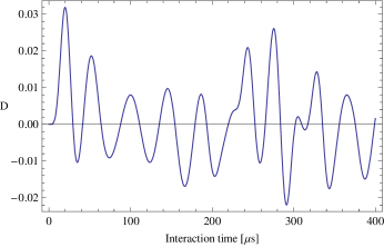
(a) $\bar{n}=2,\Delta=10$KHz

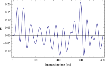
(b) $\bar{n}=2,\Delta=100$KHz

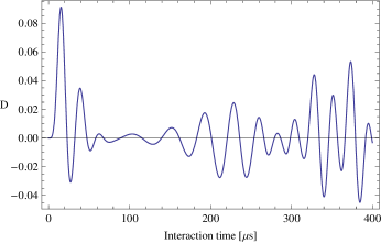
(c) $\bar{n}=5,\Delta=10$KHz

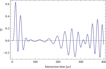
(d) $\bar{n}=5,\Delta=100$KHz

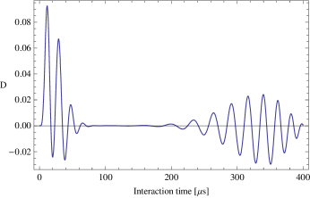
(e) $\bar{n}=10,\Delta=10$KHz

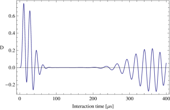
(f) $\bar{n}=10,\Delta=100$KHz

Figure 1: The determinant as a function of time for different values of the mean photon number, $\bar{n}=2$, $\bar{n}=5$, and $\bar{n}=10$ and detuning parameter, $\Delta=10$ and $\Delta=100$ KHz. In all cases $D$ has larger maximum value when $\Delta=100$KHz. The coupling constant is fixed at $g=50$KHz.

Then the expectation value of any observable $\hat{\mathcal{O}}$ of the overall system at time $t$ is

$$\langle\hat{\mathcal{O}}\rangle=\textnormal{Tr}\left(\hat{\rho}(t)\hat{\mathcal{O}}\right).$$ (3.8)

In the Appendix A we work out equations for the atom population difference $\langle\hat{\sigma}_{z}\rangle_{t}$, the average number of photons $\langle\hat{a}^{\dagger}\hat{a}\rangle_{t}$ and the correlator of these two observables $\langle\hat{\sigma}_{z}\,\hat{a}^{\dagger}\hat{a}\rangle_{t}$; see (A) – (A). Expectedly, these three quantities are linearly related to the three unknowns parameters $\langle\hat{\sigma}_{x}\rangle_{0}$, $\langle\hat{\sigma}_{y}\rangle_{0}$ and $\langle\hat{\sigma}_{z}\rangle_{0}$ of the initial atom density matrix:

$$\begin{pmatrix}\langle\hat{\sigma}_{z}\rangle_{t}\\ \langle\hat{a}^{\dagger}\hat{a}\rangle_{t}\\ \langle\hat{\sigma}_{z}\,\hat{a}^{\dagger}\hat{a}\rangle_{t}\end{pmatrix}=\mathcal{M}\begin{pmatrix}\langle\hat{\sigma}_{x}\rangle_{0}\\ \langle\hat{\sigma}_{y}\rangle_{0}\\ \langle\hat{\sigma}_{z}\rangle_{0}\end{pmatrix}+\mathcal{B},\qquad\mathcal{B}\equiv\begin{pmatrix}b_{1}\\ b_{2}\\ b_{2}\end{pmatrix}.$$ (3.9)

The elements of the matrix $\mathcal{M}$ and of the vector $\mathcal{B}$ are read off from (A) – (A); see as well Appendix A. They depend on the parameter $\alpha$ of the initial assistant state, on the parameters $\Delta$ and $g$ of the JC Hamiltonian, and on the interaction time $t$. Thus, if the determinant of $\mathcal{M}$ is not zero, one can invert $\mathcal{M}$ and express the unknown parameters of the initial atom density matrix via known quantities. Although the elements of $\mathcal{M}$ are rather complicated, the determinant itself is much simpler. It takes the explicit form

$$D\equiv{\rm det}{\mathcal{M}}= 4\Delta\,g^{2}e^{-2|\alpha|^{2}}\sum_{n=0}^{\infty}\sum_{m=0}^{\infty}\frac{|\alpha|^{2(n+m+1)}}{n!m!}(n-m)\times$$

$$\left[\frac{\sin^{2}\left(\frac{\Omega_{n}\,t}{2}\right)\,\,\sin\Omega_{m}\,t}{\Omega_{n}^{2}\Omega_{m}}-\frac{\sin^{2}\left(\frac{\Omega_{m}\,t}{2}\right)\,\,\sin\Omega_{n}\,t}{\Omega_{m}^{2}\Omega_{n}}\right],$$

where $\Omega_{n}$ is the corresponding Rabi frequency

$$\Omega_{n}=\sqrt{4(n+1)g^{2}+\Delta^{2}}.$$ (3.11)

Eq. (3) is our basic result. At the initial time $t=0$, the determinant $D$ is zero, since the initial state of the overall system is factorized. It is seen in Figs. 1.(a)–1.(f) that for a non-zero detuning, $\Delta\neq 0$, the determinant $D$ is non-zero for a certain initial period $t>0$. (Obviously $D$ is zero when there is no photon in the cavity.) Comparing figures Fig. 1.(a) and Fig. 1.(c) we see that although higher initial photon numbers $\bar{n}$ lead to bigger values for the determinant, they cause rapid oscillations in the value of $D$. This makes the measurement process more difficult. (Note in this context that the determinant depends on the absolute value of $\alpha$.)

If the average number of photons $\bar{n}=|\alpha|^{2}$ in the initial state of the field is sufficiently large, $D$ collapses to zero for intermediate times; see Figs. 1.(e) and 1.(f). The reason for this collapse is apparent from (3) and has the same origin as the collapse of the atomic population difference well known for the JCM Shore . Each term in the RHS of (3) oscillates with a different frequency. With time these oscillations get out of phase and $D$ vanishes (collapses). However, since the number of relevant oscillations in $D$ is finite, they partially get in phase for later times producing the revival of $D$, as seen in the Figs. 1.(e) and 1.(f).

It is seen that $D$ does not depend on separate frequencies $\omega$ and $\nu$ of the two-level system and the field, only their difference $\Delta=\omega-\nu$ is relevant. This is due to the choice of the measurement basis—see the LHS of (3.9)—that involves quantities which are constants of motion for $g\to 0$. Note that $D=0$ for $\Delta=0$. Thus some non-zero detuning is crucial for the present scheme of the state determination. The value of $D$ changes by varying the detuning parameter $\Delta$. Comparing the figures Fig. 1.(a) with Fig. 1.(b), Fig. 1.(c) with Fig. 1.(d), and Fig. 1.(e) with Fig. 1.(f) one observes that the value of the highest pick of $D$ increases by an order of magnitude when the detuning parameter changes from 10KHz to 100KHz. Note that in Eq. (3) for the determinant $D$ the contribution from the diagonal $n=m$ matrix elements of the assistant initial state $|\alpha\rangle\langle\alpha|$ cancels out. Thus, it is important to have an initial state of the assistant with non-zero diagonal elements in the $\{|n\rangle\}$ basis.

The basic message of this section is that the determinant $D(t)$ is not zero for a realistic range of the parameters. This means that the initial unknown state of the two level system can be determined by specifying the average atom population difference $\langle\hat{\sigma}_{z}\rangle_{t}$, the average number of photons $\langle\hat{a}^{\dagger}\hat{a}\rangle_{t}$, and their correlator $\langle\hat{\sigma}_{z}\,\hat{a}^{\dagger}\hat{a}\rangle_{t}$. In their turn these quantities are obtained from measuring two commuting observables: the atom population difference $\hat{\sigma}_{z}$ and the photon number $\hat{a}^{\dagger}\hat{a}$. Having at hand the proper measurement data for these two observables, one can trivially calculate $\langle\hat{\sigma}_{z}\rangle_{t}$, $\langle\hat{a}^{\dagger}\hat{a}\rangle_{t}$, and find $\langle\hat{\sigma}_{z}\,\hat{a}^{\dagger}\hat{a}\rangle_{t}$ via the number of coincidences.

3..0.1 Numerical illustration

At this point it may be instructive to give two concrete examples on the inversion of the matrix ${\cal M}$ in (3.9).

1. Let us ssume that the average number of photons inside the cavity is two $\bar{n}=2$, the coupling constant is $g=50$ KHz, and the detuning parameter $\Delta=10$ KHz. Looking at Fig. 1(a) one sees that the determinant is maximal at (approximately) $\tau=20\mu s$. (Recall that the typical interaction time of a thermal atomic beam with the single mode of the field is of the order of $100\mu s$ Rempe2 ; Meunier .) The elements of the matrtix ${\cal M}$ and the vector ${\cal B}$ are worked out in Appendix. Inserting all these numbers into (A) - (A) one obtains

$${\cal M}^{-1}|_{\Delta=10KHz}=\left(\begin{matrix}15.183&5.59578&0.0456968\\ 1.14077&-1.3668&-1.38923\\ 1&1&0\end{matrix}\right),$$ (3.12)

$${\cal B}|_{\Delta=10KHz}=\left(\begin{matrix}-0.0557631\\ 2.05576\\ 0.0411884\end{matrix}\right).$$ (3.13)

2. For the second example we take a larger detuning: $\bar{n}=2$, $g=50$ KHz and $\Delta=100$ KHz. The proper interaction time $t=300\mu s$ is read off from Fig. 1(b) (interaction time $t\approx 18\,{\rm\mu s}$ gives somewhat smaller determinant; see Fig. 1(b)). The numerical calculation of ${\cal M}^{-1}$ and ${\cal B}$ produces:

$${\cal M}^{-1}|_{\Delta=100KHz}=\left(\begin{matrix}3.18085&1.23251&-1.15186\\ 5.92052&-4.20194&-4.52702\\ 1&1&0\end{matrix}\right),$$ (3.14)

$${\cal B}|_{\Delta=100KHz}=\left(\begin{matrix}-0.0707962\\ 2.0708\\ -0.119635\end{matrix}\right).$$ (3.15)

3..1 Random interaction time.

We saw above that the success of the presented scheme is to a large extent determined by the ability to select properly the interaction time $t$, since this ultimately should ensure a non-zero (and sufficiently large) determinant $D$ (It is clear that a small determinant will amplify numerical errors; see the next section for an example).

To quantify the robustness of the presented scheme it is reasonable to assume that there is no perfect control in choosing the interaction time. To this end let us assume that the interaction time $t$ is a random, Gaussian distributed quantity centered at $t_{0}$ with a dispersion $\sigma$. The corresponding probability distribution $P(t)$ of thus reads

$$P(t)=\frac{1}{2\pi\sigma}\,e^{-(t-t_{0})^{2}/(2\sigma)}.$$ (3.16)

One now averages the determinant $D$ over this distribution,

$$\overline{D}(t_{0})= 4\Delta\,g^{2}e^{-2|\alpha|^{2}}\sum_{n=0}^{\infty}\sum_{m=0}^{\infty}\frac{|\alpha|^{2(n+m+1)}}{n!m!}(n-m)\left[w(\Omega_{n},\Omega_{m};t_{0})-w(\Omega_{m},\Omega_{n};t_{0})\right],$$ (3.17)

where

$$w(\Omega_{n},\Omega_{m};t_{0})=$$

$$\frac{1}{4\Omega_{n}^{2}\Omega_{m}}\,\left[2e^{-\frac{\sigma}{2}{\Omega_{m}}^{2}}\,\sin[t_{0}\Omega_{m}]-e^{-\frac{\sigma}{2}(\Omega_{m}+\Omega_{n})^{2}}\sin[t_{0}(\Omega_{m}+\Omega_{n})]-e^{-\frac{\sigma}{2}(\Omega_{m}-\Omega_{n})^{2}}\sin[(\Omega_{m}-\Omega_{n})t_{0}]\right]$$ (3.18)

It is seen that the oscillations of $D(t)$ turn after averaging to exponential factors $e^{-\frac{\sigma^{2}}{2}(\Omega_{m}\pm\Omega_{n})^{2}}$ and $e^{-\frac{\sigma^{2}}{2}\Omega_{m}^{2}}$ in (3.17, 3..1), due to which the averaged determinant $\overline{D}(t_{0})$ gets suppressed for a sufficiently large “indeterminacy” $\sigma$. This suppression is illustrated in Figs. 2 (a) and 2 (b).

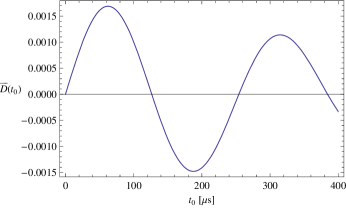
(a) $\bar{n}=2,\Delta=100$KHz, $\sigma=0.01\mu s$

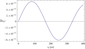
(b) $\bar{n}=2,\Delta=10$KHz, $\sigma=0.1\mu s$

Figure 2: The averaged determinant $\bar{D}$ as a function of $t_{0}$ for different values of $\sigma$; see (3.16–3..1). Here $g=50$KHz.

4 Maximum likelihood reconstruction of the initial spin state.

Above we have shown how one determines the initial spin density matrix given the three averages $\langle\hat{\sigma}_{z}\rangle_{t}$, $\langle\hat{a}^{\dagger}\hat{a}\rangle_{t}$, and $\langle\hat{\sigma}_{z}\,\hat{a}^{\dagger}\hat{a}\rangle_{t}$. However, in practice the measurement statistics that leads to the above three averages may be incomplete (due to various noises and experimental imperfections) and we should understand how to reconstruct the initial density matrix approximately given the incomplete measurement data. The general question on the approximate state reconstruction (given incomplete statistics) is of obvious importance and it got much attention in the standard schemes of quantum tomography; see hradil and references therein. Recall that in these schemes one measures non-commuting observables. In this context Refs. hradil propose to generalize suitably the classical Maximum Likelyhood (ML) method; see rao for a detailed discussion on this inference method. In particular, this generalization accounts for the fact that the (incomplete) data is obtained from measuring non-commuting observables.

Once our scheme operates by measuring the commuting variables only, we are going to show that for the approximate state reconstruction one now does not need anything beyond the most standard (classical) ML method. Since one measures the number of photons and the spin direction along the $z$-axes (these quantities are represented by the operators $\hat{a}^{\dagger}\hat{a}$ and $\hat{\sigma}_{z}$, respectively), the incomplete data in our case means that we are given frequencies $\nu_{\alpha}(m)$ of events, where one registered $m$ photons ($m=0,1,\ldots$), and where, simultaneously, the spin component assumed values $\alpha=\pm 1$. Now recall rao that in the ML method the probabilities $p_{\alpha}(m)$ (given the frequencies $\nu_{\alpha}(m)$) are obtained by maximizing over $p_{\alpha}(m)$ the likelihood function

$${\mathcal{L}}[p_{\alpha}(m)]=\sum_{\alpha=\pm 1}\sum_{m=0}^{\infty}\nu_{\alpha}(m)\ln p_{\alpha}(m).$$ (4.1)

This maximization over $p_{\alpha}(m)$ is to be carried out in the presence of relevant constraints. For our case the initial spin density matrix $\rho_{S}$ must be a positive-definite, normalized matrix; see (3.6). Thus we get a single constraint

$$\langle\hat{\sigma}_{x}\rangle_{0}^{2}+\langle\hat{\sigma}_{y}\rangle_{0}^{2}+\langle\hat{\sigma}_{z}\rangle_{0}^{2}\leq 1.$$ (4.2)

Working out (3.9) we write this constraint as a function of the probabilities $p_{\alpha}(m)$:

$$(u-\mathcal{B})^{T}\mathcal{C}(u-\mathcal{B})\leq 1,$$ (4.3)

where ^T means transposition, ${\mathcal{C}}\equiv({\mathcal{M}}{\mathcal{M}}^{T})^{-1}$, the matrix ${\mathcal{M}}$ and the vector $\mathcal{B}$ are defined in (3.9), and where finally

$$u=\begin{pmatrix}\sum_{\alpha=\pm 1}\sum_{m=0}^{\infty}\alpha p_{\alpha}(m)\\ \\ \sum_{\alpha=\pm 1}\sum_{m=0}^{\infty}mp_{\alpha}(m)\\ \\ \sum_{\alpha=\pm 1}\sum_{m=0}^{\infty}\alpha mp_{\alpha}(m)\end{pmatrix}.$$ (4.4)

If the constraint (4.3) is satisfied automatically, the maximization of ${\mathcal{L}}[p_{\alpha}(m)]$ in (4.1) produces rao

$$p_{\alpha}(m)=\nu_{\alpha}(m),$$ (4.5)

i.e., that the sought probabilities are equal to the frequencies, as one would expect intuitively. However, in general this constraint is not satisfied automatically and has to be included explicitly in the maximization of ${\mathcal{L}}[p_{\alpha}(m)]$ over $p_{\alpha}(m)$. Indeed, looking at (4.1) and (4.3) we may deduce qualitatively that the constraint (4.3) will be satisfied automatically by (4.5), if the frequencies are not very far from the actual probabilities (the ones that would be obtained in the perfect experiment) and, simultaneously, the determinant ${\rm det}{\mathcal{M}}$ is not very close to zero.

4..0.1 Numerical illustration

Below we give a concrete numerical example, where the constraint (4.3) may or may not be satisfied automatically. We take $\bar{n}=2$, $g=50$ kHz, $\Delta=100$ kHz, and we have chosen the measurement time $t=300{\rm\mu s}$ such that the corresponding determinant $D$ is maximized; see Fig. 1(b). Then we constructed the matrix $\mathcal{C}$ and the vector $\mathcal{B}$ in (4.3) [see (3.14, 3.15)], and neglecting the probabilities of having more than three photons inside the cavity, we assumed that we are given the following six frequencies $\nu_{\pm 1}(m)$ ($m=1,2,3$) normalized according to $\sum_{m=1}^{3}\sum_{\alpha=\pm 1}\nu_{\alpha}(m)=1$. For simplicity we additionally assume that these frequencies are related as

$$\nu_{1}(1)=\nu_{-1}(1),\quad\nu_{1}(2)=\nu_{-1}(2),\quad\nu_{1}(3)=\nu_{-1}(3).$$ (4.6)

For different values of $\nu_{1}(1)$, $\nu_{1}(2)$ and $\nu_{1}(3)$ the numerical maximization of (4.1) over $p_{\alpha}(m)$ under the constraint (4.3) produced a result different from (4.5) ($\sum_{m=1}^{3}\sum_{\alpha=\pm 1}p_{\alpha}(m)=1$). An example follows: for

$$\nu_{1}(1)=0.05,\quad\nu_{1}(2)=0.25,\quad\nu_{1}(3)=0.2$$ (4.7)

the probabilities are:

$$p_{1}(1)=0.05148118,\quad p_{-1}(1)=0.05087771,$$

$$p_{1}(2)=0.24811809,\quad p_{-1}(2)=0.254403426,$$

$$p_{1}(3)=0.19158279,\quad p_{-1}(3)=0.20353679.$$ (4.8)

Employing these probabilities in (4.4) and in (3.9) we get for the initial spin density matrix:

$$\hat{\rho}_{S}=\frac{1}{2}\left[1-(0.187183)\,\hat{\sigma}_{x}-(0.942992)\,\hat{\sigma}_{y}+(0.275121)\,\hat{\sigma}_{z}\right].$$ (4.9)

In this context we need to quantify the difference between the input frequencies $\nu_{\alpha}(m)$ and the probabilities $p_{\alpha}(m)$ which result from maximizing (4.1) under the constraint (4.3). In particular, this difference will quantify the relevance of the constraint (4.3) in maximizing (4.1). A good measure of distance between two probability sets is provided by rao

$$\delta[\nu||p]=1-\sum_{\alpha=\pm 1}\sum_{m=1}^{3}\sqrt{\nu_{\alpha}(m)p_{\alpha}(m)}.$$ (4.10)

This quantity is equal to its minimal value zero if (and only if) $\nu_{\alpha}(m)=p_{\alpha}(m)$ (i.e., when the constraint (4.3) holds automatically), and it is equal to its maximal value $1$ for $\nu_{\alpha}(m)p_{\alpha}(m)=0$.

In Table I we calculated the distance $\delta[\nu||p]$ between the frequencies and the corresponding probabilities. It is seen that in some cases this distance is just equal to zero, while for other cases it is rather small.

	$\nu_{1}(1)$ = 0.05	$\nu_{1}(1)$ = 0.15	$\nu_{1}(1)$ = 0.25	$\nu_{1}(1)$ = 0.30
$\nu_{1}(2)$ = 0.05	$\delta$ = 0.00989504	$\delta$ = 0.0000494347	$\delta$ = 1.1102 $\times 10^{-16}$	$\delta$ = 0.00108428
$\nu_{1}(2)$ = 0.15	$\delta$ = 0.00318619	$\delta$ = 0	$\delta$ = 0.00140516	$\delta$ = 0.0115233
$\nu_{1}(2)$ = 0.25	$\delta$ = 0.0000717018	$\delta$ = 0	$\delta$ = 0.0336704
$\nu_{1}(2)$ = 0.30	$\delta$ = 1.1102 $\times 10^{-16}$	$\delta$ = 0.0000961022

Table 1: The distance $\delta[\nu||p]$ (given by (4.10)) between the set of frequencies $\nu_{\pm 1}(m)$ and the set of corresponding probabilities $p_{\pm 1}(m)$ obtained from maximizing (4.1) under the constraint (4.3). As in the main text, we assumed that the frequencies satisfy (4.6). Thus the third frequency (not shown in the table) is got from $\mu_{\alpha}(3)=\frac{1}{2}-\mu_{\alpha}(1)-\mu_{\alpha}(2)$. The numerical values for the involved parameters are: $\bar{n}=2$ (the initial average number of photons), $g=50$ kHz (coupling constant), $\Delta=100$ kHz (detuning) and $t=300{\rm\mu s}$ (the interaction time). The matrix $\mathcal{M}$ and the vector $\mathcal{B}$ in this case are given by (3.14, 3.15). Three places in the table are empty, because the corresponding frequencies are unphysical (their sum is larger than one due to the assumption (4.6)).

5 Conclusion

In this paper we describe a method for quantum state tomography. The usual way of solving this inverse problem of quantum mechanics is to make measurements of non-commuting quantities. Single apparatus tomography proceeds differently employing controlled interaction and measuring commuting observables. This is done via coupling the system of interest to an auxiliary system (assistant) that starts its evolution from a known state. The essence of the method is that the proper coupling is able to transfer the information on the initial state of the system to a commuting basis of observables for the composite system (system+assistant).

It is important to implement the single-apparatus tomography for a situation with a physically transparent measurement base and with a realistic system-assistant interaction. Here we carried out this program for a two-level atom (system) interacting with a single mode of electromagnetic field (assistant). The atom-field interaction is given by the Jaynes-Cummings Hamiltonian, which has direct experimental realizations in quantum optics Raimond ; Haroche ; Rempe2 ; Walther1 ; Osnaghi ; Meunier , superconductivity josephson , semiconductor physics semiconductor , etc. As the measurement base we have taken presumably the simplest set of observables related to the energies of the atom and field: population difference of the atoms $\hat{\sigma}_{z}$ and the number of photons $\hat{a}^{\dagger}\hat{a}$ in the field. We have shown that one can determine the unknown initial state of the atom via post-interaction values of the average atomic population difference $\langle\hat{\sigma}_{z}\rangle$, the average number of photons $\langle\hat{a}^{\dagger}\hat{a}\rangle$ and the correlator of these quantities $\langle\hat{\sigma}_{z}\,\hat{a}^{\dagger}\hat{a}\rangle$. The latter quantity does not need a separate measurement, since it can be recovered from the simultaneous measurement of the two basic observables $\hat{\sigma}_{z}$ and $\hat{a}^{\dagger}\hat{a}$.

Since our scheme is based on measuring commuting observables, we can apply (more or less literally) the standard Maximum Likelihood setup for an approximate reconstruction of the unknown density matrix given the incomplete (noisy) measurement data. This is discussed in section 4.

Appendix A Derivation of Eq. (3).

Here we shall derive formulas for $\langle\hat{\sigma}_{z}\rangle_{t}$, $\langle\hat{a}^{\dagger}\hat{a}\rangle_{t}$ and $\langle\hat{\sigma}_{z}\,\hat{a}^{\dagger}\hat{a}\rangle_{t}$ starting from (3.1, 3.7, 2). They are used in deriving (3) and they define the matrix $\mathcal{M}$ in (3.9). One derives after straightforward algebraic steps

$$\langle\hat{\sigma}_{z}\rangle_{t}=$$

$$-2ig\langle\hat{\sigma}_{x}\rangle_{0}\sum_{n=0}^{\infty}c_{n}\frac{\sin\left(\frac{\Omega_{n}\,t}{2}\right)}{\Omega_{n}}\left\{\alpha\,\left[\cos\left(\frac{\Omega_{n}\,t}{2}\right)+i\Delta\,\frac{\sin\left(\frac{\Omega_{n}\,t}{2}\right)}{\Omega_{n}}\right]-c.c\right\}$$

$$+2g\langle\hat{\sigma}_{y}\rangle_{0}\sum_{n=0}^{\infty}c_{n}\frac{\sin\left(\frac{\Omega_{n}\,t}{2}\right)}{\Omega_{n}}\left\{\alpha\,\left[\cos\left(\frac{\Omega_{n}\,t}{2}\right)+i\Delta\,\frac{\sin\left(\frac{\Omega_{n}\,t}{2}\right)}{\Omega_{n}}\right]+c.c\right\}$$

$$+\langle\hat{\sigma}_{z}\rangle_{0}\left\{1-g^{2}\,\sum_{n=0}^{\infty}(n+1)(c_{n+1}+c_{n})\,\frac{\sin^{2}\left(\frac{\Omega_{n}\,t}{2}\right)}{\left(\frac{\Omega_{n}}{2}\right)^{2}}\right\}+b_{1},$$

where $\langle\hat{\sigma}_{i}\rangle_{0}$, $i=x,y,z$, are the unknown elements of the initial atom density matrix, $(X+{\it c.c.})$ stands for $(X+X^{*})$, and where $b_{1}$, $c_{n}$ and $\Omega_{n}$ are defined as

$$b_{1}\equiv\frac{g^{2}}{2}\sum_{n=0}^{\infty}(n+1)(c_{n+1}-c_{n})\,\frac{\sin^{2}\left(\frac{\Omega_{n}\,t}{2}\right)}{\left(\frac{\Omega_{n}}{2}\right)^{2}},$$

$$c_{n}\equiv e^{-|\alpha|^{2}}\,\frac{\alpha^{2n}}{n!},$$ (A3)

$${\Omega_{n}}^{2}\equiv 4(n+1)g^{2}+\Delta^{2}.$$ (A4)

The average number of photons in the cavity, $\hat{a}^{\dagger}\hat{a}$, can be calculated in a similar way

$$\langle\hat{a}^{\dagger}\hat{a}\rangle_{t}=$$

$$2ig\langle\hat{\sigma}_{x}\rangle_{0}\sum_{n=0}^{\infty}c_{n}\frac{\sin\left(\frac{\Omega_{n}\,t}{2}\right)}{\Omega_{n}}\left\{\alpha\,\left[\cos\left(\frac{\Omega_{n}\,t}{2}\right)+i\Delta\,\frac{\sin\left(\frac{\Omega_{n}\,t}{2}\right)}{\Omega_{n}}\right]-c.c\right\}$$

$$-2g\langle\hat{\sigma}_{y}\rangle_{0}\sum_{n=0}^{\infty}c_{n}\frac{\sin\left(\frac{\Omega_{n}\,t}{2}\right)}{\Omega_{n}}\left\{\alpha\,\left[\cos\left(\frac{\Omega_{n}\,t}{2}\right)+i\Delta\,\frac{\sin\left(\frac{\Omega_{n}\,t}{2}\right)}{\Omega_{n}}\right]+c.c\right\}$$

$$+g^{2}\langle\hat{\sigma}_{z}\rangle_{0}\sum_{n=0}^{\infty}(n+1)(c_{n+1}+c_{n})\,\frac{\sin^{2}\left(\frac{\Omega_{n}\,t}{2}\right)}{\left(\frac{\Omega_{n}}{2}\right)^{2}}+b_{2},$$

where $b_{2}$ is defined as

$$b_{2}\equiv\sum_{n=0}^{\infty}nc_{n}-\frac{g^{2}}{2}\sum_{n=0}^{\infty}(n+1)(c_{n+1}-c_{n})\,\frac{\sin^{2}\left(\frac{\Omega_{n}\,t}{2}\right)}{\left(\frac{\Omega_{n}}{2}\right)^{2}}.$$

The correlator of the two observables reads

$$\langle\hat{\sigma}_{z}\otimes\hat{a}^{\dagger}\hat{a}\rangle_{t}=$$

$$-ig\langle\hat{\sigma}_{x}\rangle_{0}\sum_{n=0}^{\infty}c_{n}(2n+1)\frac{\sin\left(\frac{\Omega_{n}\,t}{2}\right)}{\Omega_{n}}\left\{\alpha\left[\cos\left(\frac{\Omega_{n}\,t}{2}\right)+i\Delta\frac{\sin\left(\frac{\Omega_{n}\,t}{2}\right)}{\Omega_{n}}\right]-c.c\right\}$$

$$+g\langle\hat{\sigma}_{y}\rangle_{0}\sum_{n=0}^{\infty}c_{n}(2n+1)\frac{\sin\left(\frac{\Omega_{n}\,t}{2}\right)}{\Omega_{n}}\left\{\alpha\left[\cos\left(\frac{\Omega_{n}\,t}{2}\right)+i\Delta\frac{\sin\left(\frac{\Omega_{n}\,t}{2}\right)}{\Omega_{n}}\right]+c.c\right\}$$

$$+\langle\hat{\sigma}_{z}\rangle_{0}\left\{\sum_{n=0}^{\infty}nc_{n}-\frac{(n+1)g^{2}}{2}\left[(2n+3)c_{n+1}+(2n+1)c_{n}\right]\,\frac{\sin^{2}\left(\frac{\Omega_{n}\,t}{2}\right)}{\left(\frac{\Omega_{n}}{2}\right)^{2}}\right\}+b_{3},$$

where $b_{3}$ is defined as

$$b_{3}\equiv\frac{g^{2}}{4}\sum_{n=0}^{\infty}(n+1)\left[(2n+3)c_{n+1}-(2n+1)c_{n}\right]\,\frac{\sin^{2}\left(\frac{\Omega_{n}\,t}{2}\right)}{\left(\frac{\Omega_{n}}{2}\right)^{2}}.$$

References

- (1) W. de Muynck, Foundations of Quantum Mechanics, an Empiricist Approach , (Kluwer Academic Publishers, 2002).
- (2) W. Pauli, Handbuch der Physik, edited by H. Geiger and K. Scheel (Springer, Berlin, 1933), English translation: General Principles of Quantum Mechanics (Springer-Verlag, Berlin, 1980).
- (3) W. Band and J. L. Park Found. Phys. 1, 133 (1970); W. Stulpe and M. Singer, Found. Phys 3, 153 (1990); S. Weigert, Phys. Rev. A 45, 7688 (1992); R. T. Thew, K. Nemoto, A. G. White, and W. J. Munro, Phys. Rev. A 66 012303 (2002); U. Leonhardt, H. Paul, and G. M. D’Ariano, Phys. Rev. A 52, 4899 (1995).
- (4) If there is some additional information on the state, one can employ a smaller set of measurement. See, e.g., I. D. Ivanović, J. Phys. A 14 3241 (1981); W. K. Wootters and B. D. Fields, Annals of Physics 191, 363 (1989).
- (5) M. A. Nielsen and I. L. Chuang, Quantum Computation and Quantum Information (Cambridge University Press, Cambridge, England, 2000).
- (6) H. Bechmann-Pasquinucci and W. Tittel, Phys. Rev. A 61, 062308 (2000); H. Bechmann-Pasquinucci and A. Peres, Phys. Rev. Lett 85, 3313 (2000).
- (7) G. M. D’ Ariano, Phys. Lett. A 300, 1 (2002).
- (8) A. E. Allahverdyan, R. Balian, and Th. M. Nieuwenhuizen, Phys. Rev. Lett. 92, 120402-1 (2004).
- (9) X. Peng, J. Du, and D. Suter, Phys. Rev. A, 76, 042117 (2007).
- (10) E. T. Jaynes and F. W. Cummings, Proc. IEEE 51, 89 (1963).
- (11) S. Stenholm, Phys. Rep 6C, 1 (1973).
- (12) B. W. Shore and P. L. Knight, J. Mod. Opt. 40, 1195(1993).
- (13) J. M. Raimond, M. Brune, and S. Haroche, Rev. Mod. Phys. 73, 565(2001).
- (14) F. W. Cummings, Phys. Rev. 140, A1051(1965).
- (15) J. H. Eberly, N. B. Narozhny, and J. J. Sanchez-Mondragon, Phys. Rev. Lett. 44, 1323 (1980).
- (16) S. Haroche and J. M. Raimond in Advances in Atomic and Molecular Physics, edited by D. Bates and B. Bederson (Academic, New York, 1985), Vol 20, p. 350; J. A. C. Gallas et al., ibid P. 414.
- (17) G. Rempe, H. Walther, and N. Klein, Phys. Rev. lett. 58, 353 (1987).
- (18) H. Walther, Phys. Scr. T23, 165 (1988).
- (19) S. Osnaghi, et al., Phys. Rev. Lett. 87, 037902(2001).
- (20) T. Meunier, et al., phys. Rev. Lett. 94, 010401(2005).
- (21) P. Domokos, J. M. Raimond, M. Brune, and S. Haroche, Phys. Rev. A 52, 3554(1995).
- (22) D. Ellinas and I. Smyrnakis, J. Opt. B 7, S152(2005).
- (23) A. Kundu, Theor. Math. Phys 144, 975 (2005).
- (24) I. Chiorescu et al., Nature 431, 159 (2004); N. Hatakenaka, and S. Kurihara, Phys. Rev. A 54, 1729 (1996); A. T. Sornborger, A. N. Cleland, and M. R. Geller, Phys. Rev. A 70, 052315 (2004).
- (25) K. Hennessy et. al, Nature 445, 896 (2007).
- (26) V. Hussin and L. M. Nieto, J. Math. Phys. 46, 122102 (2005).
- (27) B. M. Rodríguez-Lara, H. Moya-Cessa, and A. B. Klimov, Phys. Rev. A 71, 023811 (2005).
- (28) S. Haroche, and J. M. Raimond, Cavity Quantum Electrodynamics,edited by P. Berman (Academic Press, 1994); G. Raithel et al. ibid.
- (29) H. Walther et al Rep. Prog. Phys. 69, 1325 (2006).
- (30) P. Goy, J. M. Raimond, M. Gross, and S. Haroche, Phys. Rev.Lett 50, 1903 (1983).
- (31) M.D. Crisp, Phys. Rev. A 43, 2430 (1991).
- (32) R. J. Glauber, in Quantum Optics and Electronics, Proceedings of the Les Houches Summer School, 1964, edited by C. deWitt, A. Blandin, and C. Cohen-Tannoudji (Gordon and Breach, New York, 1965), p. 63.
- (33) Z. Hradil, J. Summhammer and H. Rauch, Phys. Lett. A 261, 20 (1999); Z. Hradil, J. Summhammer, G. Badurek and H. Rauch, Phys. Rev. A 62, 014101 (2000).
- (34) R.C. Rao, Linear Statistical Inference and its Applications (NY, Wiley, 1973).