Abstract

We construct an inflation model with inflaton non-minimally coupled to gravity on a warped DGP brane. Using an exponential potential, we calculate scalar power spectrum, spectral index and the running of the spectral index. We show that for a suitable range of non-minimal coupling it is possible to exit the inflationary phase spontaneously and without any mechanism, even in the case that minimal inflation can not exit spontaneously. By a detailed analysis of parameter space, we study the constraints imposed on the non-minimal coupling from recent observational data.
PACS: 04.50.+h,  98.80.-k
Key Words: Scalar-Tensor Gravity, DGP Model, Inflation

1 Introduction

Inflation is one of the most important achievements in modern cosmology[1]. It has became the standard scenario for the early universe since it has the potential to solve some outstanding problems present in the standard Hot Big-Bang cosmology. More importantly, it produces the cosmological fluctuations for the formation of the structure that we observe today. Despite the great successes of inflation paradigm, there are several serious problems with no concrete solutions; natural realization of inflation in a fundamental theory, cosmological constant and dark energy problem, unexpected low power spectrum at large scales and egregious running of spectral index are some of these problems( for a list of theoretical problems in inflation paradigm, see [2]). Another unsolved problem in the spirit of inflationary scenario is that we do not know how to integrate it with ideas in particle physics. For example, we would like to identify the inflaton, the scalar field that drives inflation, with one of the known fields of particle physics. Furthermore, it is important that the inflaton potential emerges naturally from underling fundamental theory[3].

In the spirit of the braneworld scenarios, there are promising evidences to overcome some of these difficulties. Brane models are inspired from M/string theory and branes are topological solitons in nonperturbative M/string theories in $10$ or $11$ dimensional spacetime. As Horava and Witten have shown, gauge fields of the standard model are confined on two $9$-branes located at the end points of an $S_{1}/Z_{2}$ orbifold[4]. Based on the Horava-Witten model, the idea that our universe is a 3-brane embedded in a higher dimensional spacetime has received a great deal of attention in recent years(see [5] and references therein). In the braneworld scenario, the standard model particles are confined on the 3-brane, while the gravitation can propagate in the whole space. Since string theory claims to give us a fundamental description of the nature, it is important to study what kind of cosmology it predicts. Furthermore, despite the fact that inflationary models have been analyzed in standard four-dimensional cosmology, it is challenging to discuss them in alternative gravitational theories such as brane gravity. Among various braneworld scenarios, the model proposed by Dvali, Gabadadze and Porrati (DGP) [6] is different in this respect that it predicts deviations from the standard $4$-dimensional gravity even over large distances. In this scenario, the transition between four and higher-dimensional gravitational potentials arises due to the presence of both the brane and bulk Einstein terms in the action. Existence of a higher dimensional embedding space allows for the existence of bulk or brane matter which can certainly influence the cosmological evolution on the brane. In the DGP model, the bulk is a flat Minkowski spacetime, but a reduced gravity term appears on the brane without tension. Maeda, Mizuno and Torii have constructed a braneworld scenario which combines the Randall-Sundrum II ( RS II) model and DGP model[7]. In this combination, an induced curvature term appears on the brane in the RS II model. This model has been called warped DGP braneworld in literature[8]. Braneworld model with scalar field minimally or non-minimally coupled to gravity have been studied extensively(see[9] and references therein). The introduction of non-minimal coupling is not just a matter of taste; it is forced upon us in many situations of physical and cosmological interests such as quantum corrections to the scalar field theory and its renormalizability in curved spacetime[10]. In the spirit of braneworld inflation scenario, there are numerous studies which we highlight some of these studies based on their importance and relevance to present work. The chaotic inflation model on the RS II brane has been studied by Maartens et al[11]. The inflation model in the braneworld scenario with a Gauss-Bonnet term in the bulk has been discussed by Lidsey and Nunes [12]. Scalar perturbation from braneworld inflation has been studied by Koyama et al[13]. Barnaby, Burgess and Cline have studied warped reheating in brane-antibrane inflation[14]. Brane inflation and the cosmic string tension in superstring theory has been studied by Firouzjahi and Henry Tye[15]. Curvaton reheating mechanism in inflation on the warped DGP brane has been studied by Zhang and Zhu[16]. Huang, Li and She have used WMAP three years data to constrain brane inflation models[17]. Very recently, Bean et al have compared brane inflation with WMAP data[18]. Panotopoulos has studied assisted chaotic inflation in braneworld cosmology[19]. In addition to these studies, there are several other extensive studies in braneworld inflation which can be obtained in literature(for a recent but uncomplete list see[19]). Here we are going to investigate non-minimal inflation in warped DGP braneworld. In this direction, inflation model with minimally coupled scalar field on the warped DGP braneworld has been studied by Cai and Zhang[8]. Recently, Non-minimal inflation and running of the spectral index have been studied by Li in usual 4-dimensional spacetime[20]. This study which is restricted to 4-dimensional cosmology, has been extended to high derivative coupling by Chen et al[21]. The issue of non-minimal inflation on a warped DGP brane has not been studied yet and therefore our goal in this paper is to do this end to fill the existing gap. We study an inflation model on the warped DGP scenario where inflaton is non-minimally coupled to induced Ricci scalar on the brane. We calculate parameters of our inflation model to study implications and predictions of the model. We assume inflation of the universe is driven by a single scalar field non-minimally coupled to induced gravity with exponential potential on the warped DGP brane. We show that the inflationary phase can exit spontaneously by a suitable choice of non-minimal coupling. As we will show, depending on the values of non-minimal coupling, the running of the scalar spectral index can take negative values, which is in agreement with high precision observations of WMAP[22]. We study the constraints imposed on non-minimal coupling from observational data. As Faraoni has shown, with non-minimal coupling it is harder to achieve inflation and accelerated expansion[10]. However, since inclusion of non-minimal coupling is forced upon us from quantum field theory considerations in curved space, it is interesting to study the effect of non-minimally coupled inflaton on a warped DGP brane.

2 Warped DGP Braneworld

Consider a 5-dimensional bulk spacetime with a single 4-dimensional brane, on which gravity is localized. We write the action of our model as follows[7]

$${\cal{S}}=\int_{bulk}d^{5}X\sqrt{-{}^{(5)}g}\bigg{[}\frac{1}{2\kappa_{5}^{2}}{}^{(5)}R+{}^{(5)}{\cal{L}}_{m}\bigg{]}+\int_{brane}d^{4}x\sqrt{-g}\bigg{[}\frac{1}{\kappa_{5}^{2}}K^{\pm}+{\cal{L}}_{brane}(g_{\alpha\beta},\psi)\bigg{]}.$$ (1)

In this action the quantities are defined as follows: $X^{A}$ with $A=0,1,2,3,5$ are coordinates in bulk while $x^{\mu}$ with $\mu=0,1,2,3$ are induced coordinates on the brane. $\kappa_{5}^{2}$ is 5-dimensional gravitational constant. ${}^{(5)}R$ and ${}^{(5)}{\cal{L}}_{m}$ are 5-dimensional Ricci scalar and matter Lagrangian respectively. $K^{\pm}$ is trace of extrinsic curvature on either side of the brane. This term is known as York-Gibbons-Hawking term[23]. ${\cal{L}}_{brane}(g_{\alpha\beta},\psi)$ is the effective 4-dimensional Lagrangian. This action is actually a combination of Randall-Sundrum II model[24] and DGP model[25]. In other words, an induced curvature term is appeared on the brane in Randall-Sundrum II model. So, this model is called Warped DGP Braneworld [8]. Consider the brane Lagrangian as follows

$${\cal{L}}_{brane}(g_{\alpha\beta},\psi)=\frac{\mu^{2}}{2}R-\lambda+L_{m}$$ (2)

where $\mu$ is a mass parameter, $R$ is Ricci scalar of the brane, $\lambda$ is tension of the brane and $L_{m}$ is Lagrangian of the other matters localized on the brane. Assume that bulk contains only a cosmological constant, ${}^{(5)}\Lambda$. With these choices, action (1) gives either a generalized DGP or a generalized RS II model: it gives DGP model if $\lambda=0$ and ${}^{(5)}\Lambda=0$ and gives RS II model if $\mu=0$ [7].

Considering a flat FRW metric on the brane, the dynamical equation of the brane is given by

$$H^{2}=\frac{1}{3\mu^{2}}\bigg{[}\rho+\rho_{0}\Big{(}1+\varepsilon{\cal{A}}(\rho,a)\Big{)}\bigg{]},$$ (3)

where $\varepsilon=\pm 1$ corresponding to two possible branches of solutions in this warped DGP model and ${\cal{A}}=\bigg{[}{\cal{A}}_{0}^{2}+\frac{2\eta}{\rho_{0}}\Big{(}\rho-\mu^{2}\frac{{\cal{E}}_{0}}{a^{4}}\Big{)}\bigg{]}^{1/2}$ where    ${\cal{A}}_{0}\equiv\bigg{[}1-2\eta\frac{\mu^{2}\Lambda}{\rho_{0}}\bigg{]}^{1/2}$,   $\eta\equiv\frac{6m_{5}^{6}}{\rho_{0}\mu^{2}}$   with $0<\eta\leq 1$   and   $\rho_{0}\equiv m_{\lambda}^{4}+6\frac{m_{5}^{6}}{\mu^{2}}$. Note that ${\cal{E}}_{0}$ is an integration constant and corresponding term in the generalized Friedmann equation is called dark radiation term. Since we are interested in the inflation dynamics of our model, we neglect dark radiation term in which follows. In this case, generalized Friedmann equation (3) attains the following form

$$H^{2}=\frac{1}{3\mu^{2}}\bigg{[}\rho+\rho_{0}+\varepsilon\rho_{0}\Big{(}{\cal{A}}_{0}^{2}+\frac{2\eta\rho}{\rho_{0}}\Big{)}^{1/2}\bigg{]}.$$ (4)

This equation is the basis of our forthcoming arguments.

3 Non-Minimal Inflation

Minimal inflation on a warped DGP brane has been studied by Cai and Zhang [8]. Here we consider the case of non-minimal inflation in a warped DGP braneworld scenario described in the previous section. We assume that the inflation is driven by non-minimally coupled scalar field, $\varphi$ with potential $V(\varphi)$ on the warped DGP brane. The action of this non-minimally coupled scalar field is given by the following relation

$${\cal{S}}_{\varphi}=\int_{brane}d^{4}x\sqrt{-g}\Big{[}\frac{1}{2}\xi R\varphi^{2}-\frac{1}{2}\partial_{\mu}\varphi\partial^{\mu}\varphi-V(\varphi)\Big{]}$$ (5)

where $\xi$ is a non-minimal coupling and $R$ is Ricci scalar of the brane. Variation of the action with respect to $\varphi$ gives the equation of motion of the scalar field

$$\ddot{\varphi}+3H\dot{\varphi}-\xi R\varphi+\frac{dV}{d\varphi}=0.$$ (6)

The energy density and pressure of the non-minimally coupled scalar field are given by

$$\rho=\frac{1}{2}\dot{\varphi}^{2}+V(\varphi)-6\xi R\varphi H\dot{\varphi},$$ (7)

$$p=\frac{1}{2}\dot{\varphi}^{2}-V(\varphi)+2\big{(}\xi R\varphi\ddot{\varphi}+2\xi R\varphi H\dot{\varphi}+\xi R\dot{\varphi}^{2}\big{)}.$$ (8)

In the slow-roll approximation where $\dot{\varphi}^{2}\ll V(\varphi)$ and $\ddot{\varphi}\ll|3H\dot{\varphi}|$, equation of motion for scalar field and energy density take the following forms respectively

$$3H\dot{\varphi}-\xi R\varphi+\frac{dV}{d\varphi}\approx 0,$$ (9)

$$\rho\approx V(\varphi)-6\xi R\varphi H\dot{\varphi}.$$ (10)

Now we define the following quantities

$$\epsilon=-\frac{\dot{H}}{H^{2}},$$ (11)

$$\delta=\frac{1}{3H^{2}}\frac{d^{2}V}{d\varphi^{2}},$$ (12)

$$\gamma^{2}=\frac{1}{(3H^{2})^{2}}\frac{d^{3}V}{d\varphi^{3}}\frac{dV}{d\varphi}.$$ (13)

In the slow-roll approximation, using equations (4), (6) and (10) we find

$$\epsilon=\frac{\mu^{2}}{2}\frac{1}{\rho^{2}}\Bigg{[}\Big{(}\frac{dV}{d\varphi}\Big{)}^{2}-\xi R\frac{dV}{d\varphi}\Big{(}\varphi-\frac{dV}{d\varphi}-2\varphi\frac{d^{2}V}{d\varphi^{2}}\Big{)}-2\xi^{2}R^{2}\varphi\Big{(}3\frac{dV}{d\varphi}+\varphi\frac{d^{2}V}{d\varphi^{2}}\Big{)}+4\xi^{3}R^{3}\varphi^{2}\Bigg{]}$$

$$\times\Bigg{[}\frac{1+\varepsilon\eta\Big{(}{\cal{A}}_{0}^{2}+\frac{2\eta\rho}{\rho_{0}}\Big{)}^{-1/2}}{\bigg{(}1+\frac{\rho_{0}}{\rho}\Big{[}1+\varepsilon\Big{(}{\cal{A}}_{0}^{2}+\frac{2\eta\rho}{\rho_{0}}\Big{)}^{1/2}\Big{]}\bigg{)}^{2}}\Bigg{]},$$ (14)

where a part of the effects of non-minimal coupling is hidden in the definition of energy density, $\rho$, which attains the following form

$$\rho\approx V+2\xi R\varphi\frac{dV}{d\varphi}-2\xi^{2}R^{2}\varphi^{2}.$$ (15)

$\delta$ and $\gamma$ can be obtained similarly.

Now we consider an exponential potential defined as follows

$$V(\varphi)=V_{0}\exp{\Big{(}-\sqrt{\frac{2}{p}}\frac{\varphi}{\mu}\Big{)}},$$ (16)

where $V_{0}$ and $p$ are constants. In the minimal case where $\xi=0$, we have inflationary solution for $p>2$. However, inflation does not take place for $p\leq 2$ in the case of single scalar field. It has been shown that inflation can proceed for the case of multi-scalar fields even if the individual scalar field has the power less than unity(assisted inflation)[26].

In our non-minimal case and with this potential, the slow-roll parameters become

$$\epsilon=\frac{1}{p}\frac{1}{(1-2\sqrt{\frac{2}{p}}\,\frac{\xi R\varphi}{\mu})^{2}}\Bigg{(}1+\xi R\Big{(}\sqrt{\frac{p}{2}}\frac{\mu\varphi}{V}+1-2\sqrt{\frac{2}{p}}\frac{\varphi}{\mu}\Big{)}\Bigg{)}$$

$$\times\Bigg{[}\frac{1+\varepsilon\eta\Big{(}{\cal{A}}_{0}^{2}+2\eta x\Big{)}^{-1/2}}{\bigg{(}1+\frac{1}{x}\Big{[}1+\varepsilon\Big{(}{\cal{A}}_{0}^{2}+2\eta x\Big{)}^{1/2}\Big{]}\bigg{)}^{2}}\Bigg{]},$$ (17)

$$\delta=\frac{2}{p}\,\,\frac{x}{\Big{(}1-2\sqrt{\frac{2}{p}}\frac{\xi R\varphi}{\mu}\Big{)}\Big{[}x+1+\varepsilon\Big{(}{\cal{A}}_{0}^{2}+2\eta x\Big{)}^{1/2}\Big{]}}$$ (18)

where $x=\frac{\rho}{\rho_{0}}$ and

$$\gamma^{2}=\delta^{2}.$$ (19)

Only terms of $\cal{O}(\xi)$ have been considered in these and forthcoming calculations. Substituting (16) into (15), $\rho$ takes the following form

$$\rho\approx V\Big{(}1-2\sqrt{\frac{2}{p}}\frac{\xi R\varphi}{\mu}\Big{)}$$ (20)

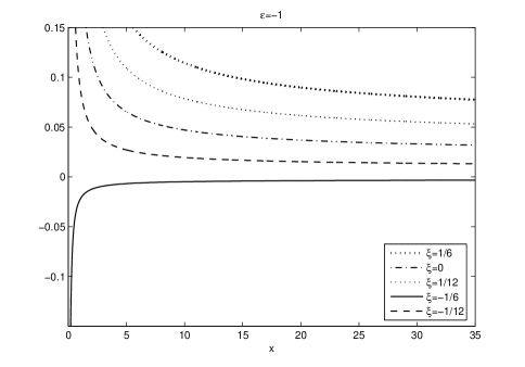
For comparison, we briefly discuss the minimal case where $\xi=0$. In this case the inflation will ends when $\epsilon=1$. The Universe enters inflationary phase where $p>2$. In this minimal case Universe can not exit inflationary phase in the branch of $\varepsilon=1$ while in the branch $\varepsilon=-1$ it can exit inflationary phase naturally without any other mechanism[8]. However, in our non-minimal case the situation is very different. Existence of non-minimal coupling provides the situation that Universe can exit inflationary phase even in branch $\varepsilon=1$. To show this end, we should solve the following complicated equations

$$\frac{1}{p}\frac{1}{(1-2\sqrt{\frac{2}{p}}\,\frac{\xi R\varphi}{\mu})^{2}}\Bigg{(}1+\xi R\Big{(}\sqrt{\frac{p}{2}}\frac{\mu\varphi}{V}+1-2\sqrt{\frac{2}{p}}\frac{\varphi}{\mu}\Big{)}\Bigg{)}$$

$$\times\Bigg{[}\frac{1+\eta\Big{(}{\cal{A}}_{0}^{2}+2\eta x\Big{)}^{-1/2}}{\bigg{(}1+\frac{1}{x}\Big{[}1+\Big{(}{\cal{A}}_{0}^{2}+2\eta x\Big{)}^{1/2}\Big{]}\bigg{)}^{2}}\Bigg{]}=1,$$ (21)

for $\varepsilon=1$, and

$$\frac{1}{p}\frac{1}{(1-2\sqrt{\frac{2}{p}}\,\frac{\xi R\varphi}{\mu})^{2}}\Bigg{(}1+\xi R\Big{(}\sqrt{\frac{p}{2}}\frac{\mu\varphi}{V}+1-2\sqrt{\frac{2}{p}}\frac{\varphi}{\mu}\Big{)}\Bigg{)}$$

$$\times\Bigg{[}\frac{1-\eta\Big{(}{\cal{A}}_{0}^{2}+2\eta x\Big{)}^{-1/2}}{\bigg{(}1+\frac{1}{x}\Big{[}1-\Big{(}{\cal{A}}_{0}^{2}+2\eta x\Big{)}^{1/2}\Big{]}\bigg{)}^{2}}\Bigg{]}=1,$$ (22)

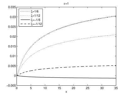
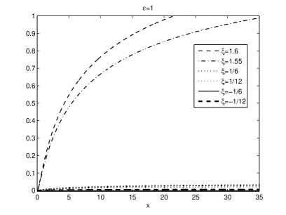
for $\varepsilon=-1$. These equations can not be solved in algebraic way, so we try to solve them numerically. As figure $1$ shows, for $\varepsilon=-1$ inflationary phase can exit without any mechanism for positive values of non-minimal coupling. Also for some small negative values of non-minimal coupling such as $\xi=-\frac{1}{12}$ this spontaneous exit is possible. However, some values of non-minimal coupling such as $\xi=-\frac{1}{6}$ prevents spontaneous exit of inflation. In fact, for all $\xi<-\frac{1}{6}$ this spontaneous exit fails in branch $\varepsilon=-1$. In the case of $\varepsilon=+1$ inflationary phase can not exit spontaneously with small (positive and negative) values of non-minimal coupling(figure $2$). However, for relatively large values of non-minimal coupling, (for instance $\xi\geq 1.55$) it is possible to exit inflationary phase spontaneously even in $\varepsilon=+1$ branch. This is the main deference of our non-minimal framework with minimal case [8]. Note that in the original DGP model, spontaneous exit of inflation is possible but inflationary phase lasts to extremely low energy scale ($\rho_{0}\sim(10^{-3}eV)^{4}$) which is evidently impossible. In our non-minimal framework this difficulty can be avoided by choosing a suitable range of non-minimal coupling.

The number of e-folds, $N\equiv\ln\frac{a_{e}}{a_{i}}$ can be written as

$$N=-\int_{\varphi_{i}}^{\varphi_{e}}3H^{2}\frac{d\varphi}{dV}d\varphi,$$ (23)

where $\varphi_{i}$ denotes the value of scalar field $\varphi$ when Universe scale observed today crosses the Hubble horizon during inflation, while $\varphi_{e}$ is the value of scalar field when the Universe exits the inflationary phase. In the presence of non-minimal coupling and with exponential potential (16), the number of e-folds is given by

$$N=\frac{1}{\mu}\,\sqrt{\frac{p}{2}}\int_{\varphi_{i}}^{\varphi_{e}}\frac{\Big{(}1-2\sqrt{\frac{2}{p}}\frac{\xi R\varphi}{\mu}\Big{)}}{x}\,\Big{[}x+1+\varepsilon\omega\Big{]}d\varphi,$$ (24)

where $\omega=\Big{(}{\cal{A}}_{0}^{2}+2\eta x\Big{)}^{1/2}$   and   $x=\frac{V\Big{(}1-2\sqrt{\frac{2}{p}}\frac{\xi R\varphi}{\mu}\Big{)}}{\rho_{0}}$   so that   $d\varphi=-\frac{dx}{\sqrt{\frac{2}{p}}\frac{1}{\mu}(x+2\frac{\xi RV}{\rho_{0}})}$ .  $x_{i}$ is the value of $x$ when the cosmic scale observed today crosses the Hubble horizon during inflation.

In the next step we consider the scalar perturbation of the metric. These perturbations are supposed to be adiabatic. We define the scalar spectrum index as follows

$$n_{s}=1+\frac{d\ln A_{s}^{2}}{d\ln k},$$ (25)

where $A_{s}$ is the scalar curvature perturbation amplitude of a given mode when re-enters the Hubble radius, defined as $A_{s}^{2}=\frac{H^{4}}{(25\pi^{2}\dot{\varphi}^{2})}$. Substituting (9) in this relation, we obtain

$$A_{s}^{2}=\Bigg{[}\frac{9H^{6}}{25\pi^{2}\Big{(}\xi R\varphi-\frac{dV}{d\varphi}\Big{)}^{2}}\Bigg{]}_{k=aH},$$ (26)

Note that although the non-minimal coupling of the scalar field to the Ricci curvature on the brane leads to the non-conservation of the scalar field effective energy density[27,28]

$$\dot{\rho}+3H(\rho+p)=-6\xi R\varphi\dot{\varphi}(H^{2}+\dot{H}),$$ (27)

since the total energy-momentum on the brane is conserved, the curvature perturbation on a uniform density hypersurface is still conserved on large scale. Using parameters of slow-rolling, we have

$$n_{s}=1-6\,\epsilon+2\delta-\frac{2}{3}\frac{\xi R}{H^{2}}.$$ (28)

The running of the spectral index is defined as follows

$$\frac{dn_{s}}{d\ln k}=16\epsilon\delta-24\epsilon^{2}+4\gamma^{2}-\frac{16}{3}\frac{\xi R}{H^{2}}\,\epsilon-\frac{4\xi R\varphi}{\frac{dV}{d\varphi}}\,\gamma^{2}.$$ (29)

For comparison purposes, we first write the explicit form of these quantities in the minimal framework where $\xi=0$  [8]

$$n_{s}=1-\frac{2}{p}\,\,\frac{x^{\prime}\Big{(}2{\cal{A}}_{0}^{2}+\eta x^{\prime}+(-2+x^{\prime})\omega\Big{)}}{\omega(1+x^{\prime}-\omega)^{2}},\hskip 284.52756pt$$ (30)

and

$$\frac{dn_{s}}{d\ln k}=\frac{8}{p^{2}}\,\,\frac{x^{\prime}\,{}^{2}}{\omega^{2}(1+x^{\prime}-\omega)^{4}}\times\hskip 312.9803pt$$

$$\Big{[}2{\cal{A}}_{0}^{4}+{\cal{A}}_{0}^{2}\Big{(}2+8x^{\prime}-4(1+2x^{\prime})\omega+3x^{\prime}\,{}^{2}+12\eta x^{\prime}\Big{)}+\eta x^{\prime}\Big{(}4+x^{\prime}(16+13\eta-14\omega)+6x^{\prime}\,{}^{2}-12\omega\Big{)}\Big{]},\hskip 56.9055pt$$ (31)

where $x^{\prime}=\frac{V}{\rho_{0}}$. However, in the presence of non-minimal coupling these quantities attain the following more complicated forms

$$n_{s}=1-\frac{2}{p}\,\,\frac{x}{(1-2\sqrt{\frac{2}{p}}\,\frac{\xi R\varphi}{\mu})(1+x+\varepsilon\omega)}\times\hskip 284.52756pt$$

$$\Bigg{[}-2+\frac{\mu^{2}\xi Rp}{V}+\frac{3x\,(1+\varepsilon\eta\omega^{-1})}{(1-2\sqrt{\frac{2}{p}}\,\frac{\xi R\varphi}{\mu})(1+x+\varepsilon\omega)}\Bigg{(}1+\xi R\Big{(}\sqrt{\frac{p}{2}}\frac{\mu\varphi}{V}+1-2\sqrt{\frac{2}{p}}\frac{\varphi}{\mu}\Big{)}\Bigg{)}\Bigg{]},\hskip 56.9055pt$$ (32)

and

$$\frac{dn_{s}}{d\ln k}=\frac{8}{p^{2}(1-2\sqrt{\frac{2}{p}}\,\frac{\xi R\varphi}{\mu})^{2}}\,\,\Big{(}\frac{x}{x+1+\varepsilon\omega}\Big{)}^{2}\times\hskip 312.9803pt$$

$$\Bigg{[}2(1+\sqrt{\frac{p}{2}}\frac{\xi R\varphi\mu}{V})+\Big{(}4-\frac{2\xi R\mu^{2}p}{V}\Big{)}\Big{(}\frac{x}{x+1+\varepsilon\omega}\Big{)}(1+\varepsilon\eta\omega^{-1})\Bigg{(}\frac{1+\xi R\Big{(}\sqrt{\frac{p}{2}}\,\frac{\mu\varphi}{V}+1-2\sqrt{\frac{2}{p}}\,\frac{\varphi}{\mu}\Big{)}}{1-2\sqrt{\frac{2}{p}}\,\frac{\xi R\varphi}{\mu}}\Bigg{)}\hskip 85.35826pt$$

$$-3\Big{(}\frac{x}{x+1+\varepsilon\omega}\Big{)}^{2}(1+\varepsilon\eta\omega^{-1})^{2}\Bigg{(}\frac{1+\xi R\Big{(}\sqrt{\frac{p}{2}}\,\frac{\mu\varphi}{V}+1-2\sqrt{\frac{2}{p}}\,\frac{\varphi}{\mu}\Big{)}}{1-2\sqrt{\frac{2}{p}}\,\frac{\xi R\varphi}{\mu}}\Bigg{)}^{2}\Bigg{]},\hskip 142.26378pt$$ (33)

where as usual   $x=\frac{V\Big{(}1-2\sqrt{\frac{2}{p}}\,\frac{\xi R\varphi}{\mu}\Big{)}}{\rho_{0}}$. The relation between $x$ and $x^{\prime}$ is

$$x=x^{\prime}\Big{(}1-2\sqrt{\frac{2}{p}}\,\frac{\xi R\varphi}{\mu}\Big{)},$$ (34)

The COBE normalization gives us $A_{s}^{2}=4\times 10^{-10}$, therefore equation (26) leads to

$$\Bigg{[}\frac{\Big{[}V\Big{(}1-2\sqrt{\frac{2}{p}}\frac{\xi R\varphi}{\mu}\Big{)}+\rho_{0}+\varepsilon\rho_{0}\Big{(}{\cal{A}}_{0}^{2}+\frac{2\eta\rho}{\rho_{0}}\Big{)}^{1/2}\Big{]}^{3}}{75\pi^{2}\mu^{6}\Big{(}\xi R\varphi+\sqrt{\frac{2}{p}}\,\frac{1}{\mu}V\Big{)}^{2}}\Bigg{]}_{k=aH}=4\times 10^{-10}.$$ (35)

This relation can be rewritten as follows

$$\frac{\Big{(}1-2\sqrt{\frac{2}{p}}\frac{\xi R\varphi}{\mu}\Big{)}}{\Big{(}1+\sqrt{\frac{p}{2}}\,\frac{\xi R\varphi\mu}{V}\Big{)}^{\frac{2}{3}}}\times\Big{[}1+\frac{1}{x}+\frac{\varepsilon}{x}({\cal{A}}_{0}^{2}+2\eta x)^{\frac{1}{2}}\Big{]}=B$$ (36)

where   $B=(\frac{6\times 10^{-7}}{yp})^{\frac{1}{3}}$   and    $y=\frac{V_{i}}{\mu^{4}}$ . Here the subscript $i$ means that the corresponding quantity should be calculated at $k=aH$. From equation (36) we get

$$x_{i}=\frac{2(-1+D+\eta)}{(-1+D)^{2}},$$ (37)

where

$$D=B\times\frac{\Big{(}1+\sqrt{\frac{p}{2}}\,\frac{\xi R\varphi\mu}{V}\Big{)}^{\frac{2}{3}}}{\Big{(}1-2\sqrt{\frac{2}{p}}\frac{\xi R\varphi}{\mu}\Big{)}}.$$ (38)

In the minimal limit  $\xi=0$, when $y=y^{\prime}_{s}=\frac{6\times 10^{-7}}{p}$, there is a singularity that appears when $x_{i}\rightarrow\infty$ in (37) since in this case   $D=1$. This singularity restricts the energy scale of the inflation in such a way that $y<y^{\prime}_{s}$ should be satisfied. We can see that with a non-minimally coupled inflaton, the restriction on the energy scale of the inflation is a function of non-minimal coupling $\xi$ as follows

$$y<y_{s},$$ (39)

where energy scale $y_{s}$ has the following complicated non-minimal coupling dependence

$$y_{s}=(\frac{6\times 10^{-7}}{p})\times\frac{\Big{(}1+\sqrt{\frac{p}{2}}\,\frac{\xi R\varphi\mu}{V}\Big{)}^{2}}{\Big{(}1-2\sqrt{\frac{2}{p}}\frac{\xi R\varphi}{\mu}\Big{)}^{3}}.$$ (40)

If $y>y_{s}$, we have $x_{i}=\infty$ or $\varphi_{i}=\infty$. This leads to a negative number of e-folds and therefore an unphysical result. The energy scale of inflation for different values of non-minimal coupling will be discussed in the next section.
Before a detailed analysis of parameter space, we should stress that with non-minimal coupling of inflaton and curvature, one can perform a conformal transformation to a new metric for which the coupling of the inflaton to the metric becomes minimal(see for example [10, 30-33]). In the new frame(Einstein frame), the inflaton potential gets an additional term. As Komatsu and Futamase have shown[30], generally slow-roll parameters are different in these two frames (Jordan and Einstein Frame). Spectral index and other inflationary parameters are different in this frames also and only in a first order theory these quantities are the same in two frames. In our case, with non-minimally coupled inflaton on the warped DGP brane, slow-roll parameters are shown to be very different with respect to minimal case. In this case warp factor itself obtains a complicated dependence on the non-minimal coupling. To see this end, remember that ${\cal{A}}_{0}\equiv\bigg{[}1-2\eta\frac{\mu^{2}\Lambda}{\rho_{0}}\bigg{]}^{1/2}$. With non-minimally coupled inflaton, we should redefine $\eta$ as follows

$$\eta_{new}=\eta\Big{(}1-2\sqrt{\frac{2}{p}}\frac{\xi R\varphi}{\mu}\Big{)}.$$ (41)

Now we may define a new ${\cal{A}}_{0}$ as follows

$$\Big{(}{\cal{A}}_{0}\Big{)}_{new}\equiv\bigg{[}1-2\eta\Big{(}1-2\sqrt{\frac{2}{p}}\frac{\xi R\varphi}{\mu}\Big{)}\frac{\mu^{2}\Lambda}{\rho_{0}}\bigg{]}^{1/2}.$$ (42)

This equation shows an explicit dependence of warp factor to the non-minimal coupling of inflaton and Ricci scalar. As a result, with non-minimally coupled inflaton, we are not faced only with a redefinition of potential; we have a redefinition of slow-rolling parameters also. In this case physical observable such as spectral index attain a new and complicated form depending on both warp factor and non-minimal coupling as follows

$$n_{s}=1-\frac{2}{p}\,\,\frac{x}{\omega(1-2\sqrt{\frac{2}{p}}\,\frac{\xi R\varphi}{\mu})(1+x+\varepsilon\omega)^{2}}\times\hskip 284.52756pt$$

$$\Bigg{[}\omega\Bigg{(}-2-2x+3x\Bigg{(}1+\xi R\Big{(}\sqrt{\frac{p}{2}}\frac{\mu\varphi}{V}+1-2\sqrt{\frac{2}{p}}\frac{\varphi}{\mu}\Big{)}\Bigg{)}\Bigg{)}+\frac{\mu^{2}\xi Rp}{V}\Big{(}\omega(1+x)+\varepsilon({\cal{A}}_{0}^{2}+2\eta x)\Big{)}-$$

$$\varepsilon\Bigg{(}2{\cal{A}}_{0}^{2}+4\eta x-3\eta x\Bigg{(}1+\xi R\Big{(}\sqrt{\frac{p}{2}}\frac{\mu\varphi}{V}+1-2\sqrt{\frac{2}{p}}\frac{\varphi}{\mu}\Big{)}\Bigg{)}\Bigg{)}\Bigg{]}\hskip 142.26378pt$$ (43)

In fact as has been shown in [30], only for $\xi\gg 1$ physical observables of inflation do not depend on $\xi$. Therefore, in our case both warp factor and observable quantities are different relative to minimal case and a frame (conformal) transformation alone cannot relate our results to the results of minimal case studied in [8].
With this point in mind, in the next section we present a detailed analysis of parameter space. In which follows, in all numerical calculations and resulting figures we have set $\mu=\varphi=R={\cal{A}}_{0}=V_{0}=1$,  $p=50$ and $\eta=0.99$.

4 Numerical Analysis of the Parameter Space

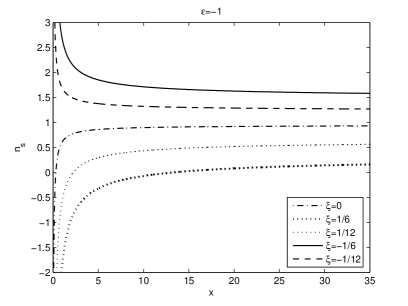
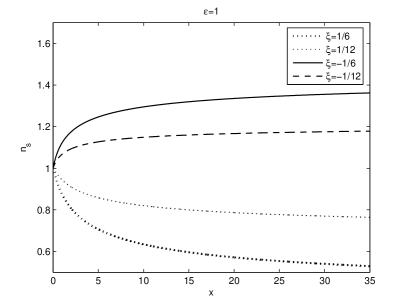
To explore cosmological implications of this non-minimal inflation model, we perform some numerical analysis of parameter space. The results of this analysis are shown in figures. Figure $1$ shows the variation of the slow roll parameter $\epsilon$ with respect to $x$ for different values of non-minimal coupling on the branch $\varepsilon=-1$ of the warped DGP braneworld. In minimal case, inflation on this branch can exit spontaneously without any mechanism since the equation $\epsilon=1$ has solution always. As this figure shows, the situation for non-minimal case is different in some respects. For example, if $\xi=-\frac{1}{6}$, it is impossible to reach $\epsilon=1$ and therefore, there is no spontaneous exit from inflation with this non-minimal coupling within our framework. For negative larger values of non-minimal coupling the situation is similar. Therefore, in contrast to minimal inflation on the warped DGP brane, non-minimal inflation prevents spontaneous exit from inflation on the $\varepsilon=-1$ branch for some values of non-minimal coupling. Note that in this figure all upper curves intersect $\epsilon=1$ line, but the lower curve corresponding to $\xi=-\frac{1}{6}$ will not reach $\epsilon=1$ at all. Figure $2$ shows the slow roll parameter $\epsilon$ versus $x=\frac{V\Big{(}1-2\sqrt{\frac{2}{p}}\,\frac{\xi R\varphi}{\mu}\Big{)}}{\rho_{0}}$ for different values of non-minimal coupling on the branch $\varepsilon=+1$ of the warped DGP braneworld. As this figure shows, for small values of non-minimal coupling it is impossible to exit inflationary phase spontaneously and within reasonable time scale. However, for larger values of non-minimal coupling, in contrast to minimal case[8], it is possible to exit from inflation spontaneously in branch $\varepsilon=+1$ with some values of the non-minimal coupling in a reasonable time scale. For instance, as figure $3$ shows, if we set $\xi=1.55$ or larger, it is possible to reach $\epsilon=1$ in this branch. This is one of the main differences between our model and the minimal model studied in [8]. Figure $4$ shows the scalar spectrum index with $\varepsilon=-1$. In minimal case, this index is always less than unity(red spectrum)[8]. We see that for negative non-minimal coupling it is possible to find scalar spectrum index larger than unity(a blue spectrum). The result of WMAP3 for $\Lambda$CDM gives $n_{s}=0.951^{+0.015}_{-0.019}$ for index of the power spectrum[29]. Combining WMAP3 with SDSS (Sloan Digital Sky Survey), gives $n_{s}=0.948^{+0.015}_{-0.018}$ at the level of one standard deviation[17]. These results show that a red power spectrum is favored at least at the level of two standard deviations. If there is running of the spectral index, the constraints on the spectral index and its running are given by

$$n_{s}=1.21^{+0.13}_{-0.16}$$ (44)

and

$$\frac{dn_{s}}{d\ln k}=-0.102^{+0.050}_{-0.043}$$ (45)

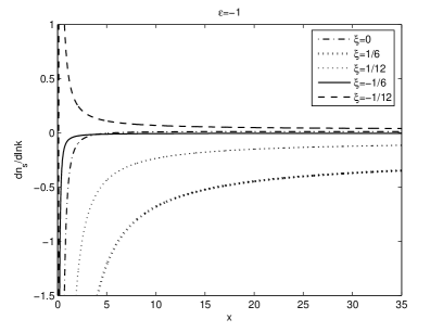
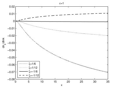
We see from figure $4$ that in our non-minimal case, for some negative values of non-minimal coupling it is possible to have spectral index such that $n_{s}>1$. Therefore our non-minimal inflation model is consistent with WMAP3 data with running of spectral index. In other words, non-minimal inflation can be supported by WMAP3 data with running of spectral index. The situation for $\varepsilon=+1$ is similar. The main characteristic of our setting in this regard is the fact that now $n_{s}>1$ is possible for some values of non-minimal coupling. This situation is impossible in minimal inflation on the warp DGP brane. On the other hand, the running of the spectral index in minimal case is always negative. In our non-minimal case, as figure $6$ with $\varepsilon=-1$ shows, for small negative values of non-minimal coupling (for instance, $\xi=-\frac{1}{12}$), it is possible to have positive running of the spectral index. Therefore, in contrast to minimal case, for a suitable range of non-minimal coupling running of spectral index can attain large positive values. The situation for branch $\varepsilon=+1$ is more or less similar (figure $7$), however in this branch the running of the scalar spectrum index for conformal coupling is approximately zero.

Now we investigate the energy scale of this non-minimal inflation. We set $\eta=0.99$ and calculate the energy scales for different values of non-minimal coupling. Firstly we should obtain $V_{i}$’s using $y=\frac{V_{i}}{\mu^{4}}$ for different values of non-minimal coupling. Considering $\rho\approx V\Big{(}1-2\sqrt{\frac{2}{p}}\frac{\xi R\varphi}{\mu}\Big{)}$, we obtain the energy scales of this non-minimal inflation as presented in table 1.

Table 1: Energy Scales of Non-minimal Inflation

		$V_{i}$	$\rho_{i}$
$\xi=\frac{1}{6}$	$y\sim 10^{-8}$	$(10^{15}GeV)^{4}$	$(0.98\times 10^{15}GeV)^{4}$
$\xi=\frac{1}{12}$	$y\sim 10^{-8}$	$(10^{15}GeV)^{4}$	$(0.99\times 10^{15}GeV)^{4}$
$\xi=-\frac{1}{6}$	$y\sim 10^{-12}$	$(10^{14}GeV)^{4}$	$(1.01\times 10^{14}GeV)^{4}$
$\xi=-\frac{1}{12}$	$y\sim 10^{-9}$	$(5.62\times 10^{14}GeV)^{4}$	$(5.66\times 10^{14}GeV)^{4}$

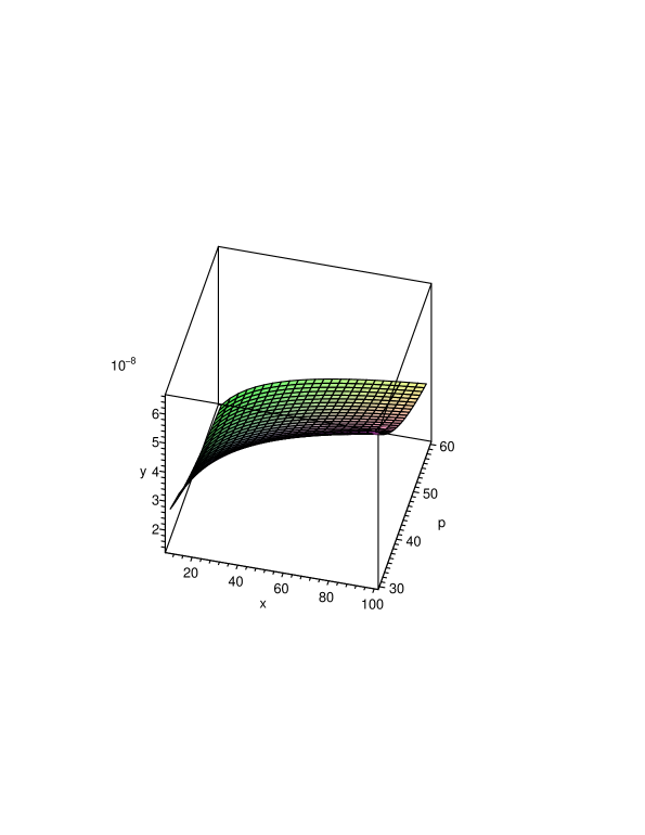
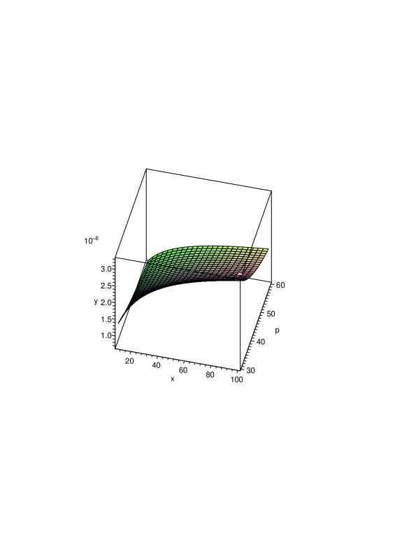
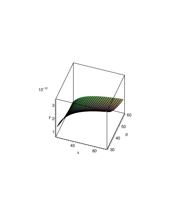
For comparison, note that in the minimal case we have $\rho_{i}\sim(5.62\times 10^{14}GeV)^{4}$, therefore except for $\xi=-\frac{1}{6}$, the non-minimal coupling leads to larger values of energy scales of inflation. Figures $8$, $9$, $10$ and $11$ show the non-minimal inflation energy scale versus the parameters $x$ and $p$ for different values of non-minimal coupling. Increasing the values that a positive non-minimal coupling can attains leads to the larger inflation energy scale. The situation for negative non-minimal coupling is similar. Since based on WMAP3 data, $n_{s}=1.21^{+0.13}_{-0.16}$, or $1.05\leq n_{s}\leq 1.34$, using equation (32), (34) and with $\rho_{\circ}\sim(10^{-3}eV)^{4}$, the constraint on the non-minimal coupling from WMAP3 data are  $\xi\leq-1.05\times 10^{-1}$  and  $\xi\geq 1.2\times 10^{-2}$.
In summary, inclusion of non-minimal coupling in inflation paradigm is forced upon us from quantum field theory considerations in curved space. In this paper we have studied non-minimal inflation on a warped DGP braneworld. We have presented full dynamics of slow-roll equations with non-minimally coupled scalar field and consistency of the numerical results with observational data from WMAP3. Our model allows for spontaneous exit from inflationary phase with some values of non-minimal coupling and without any mechanism. Even for situations that minimal case can not provide spontaneous exit, non-minimal coupling can be chosen suitably to exit inflationary phase spontaneously. This non-minimal model provides scalar spectrum index larger than unity and also large positive values of running of the spectral index. Finally, energy scale of inflation with non-minimally coupled inflaton is larger than minimal case(except for $\xi=-\frac{1}{6}$).

Acknowledgement
A part of this work has been done during KN sabbatical leave at Durham University, UK. He would like to appreciate members of the Centre for Particle Theory of Durham University, specially Professor Ruth Gregory, for kind hospitality. We would also to appreciate a referee for His/Her valuable comments.

Figure 1: Variation of $\epsilon$ for different values of non-minimal coupling for branch $\varepsilon=-1$.

Figure 2: Variation of $\epsilon$ for different values of non-minimal coupling for branch $\varepsilon=+1$.

Figure 3: Variation of $\epsilon$ for different values of non-minimal coupling for branch $\varepsilon=+1$. For $\xi>1.55$ it is possible to exit inflationary phase spontaneously without any mechanism.

Figure 4: Spectral index $n_{s}$ for branch $\varepsilon=-1$.

Figure 5: Spectral index $n_{s}$ for branch $\varepsilon=+1$.

Figure 6: Running of the spectral index, $\frac{dn_{s}}{d\ln{k}}$ for branch $\varepsilon=-1$.

Figure 7: Running of the spectral index, $\frac{dn_{s}}{d\ln{k}}$ for branch $\varepsilon=+1$

Figure 8: Energy Scale of Non-Minimal Inflation with $\xi=\frac{1}{6}$                                                                                                          

Figure 9: $\xi=\frac{1}{12}$

Figure 10: $\xi=-\frac{1}{6}$                                                                                                         

Figure 11: $\xi=-\frac{1}{12}$

References

- [1] A. Liddle and D. Lyth, Cosmological Inflation and Large-Scale Structure, Cambridge University Press, 2000
- [2] R. H. Brandenberger, [arXiv:hep-th/0509099]
- [3] J. E. Lidsey et al, Rev. Mod. Phys. 69 (1997) 373
- [4] P. Horava and E. Witten, Nucl. Phys. B 460 (1996) 506
- [5] R. Maartens, Living Rev. Relativity, 7 (2004) 7, http://www.livingreviews.org/lrr-2004-7 and references therein
- [6] G. Dvali, G. Gabadadze and M. Porrati, Phys. Lett. B 485 (2000) 208, [arXiv:hep-th/0005016]
- [7] Kei-ichi Maeda, S. Mizuno and T. Torii, Phys. Rev. D 68 (2003) 024033, [arXiv:gr-qc/0303039]
- [8] R.-G. Cai and H. Zhang, JCAP 08 (2004) 017, [arXiv:hep-th/0403234]
- [9] K. Nozari, Phys. Lett. B 652 (2007) 159-164, [arXiv:hep-th/07070719]
-
[10]
V. Faraoni, Phys. Rev. D 53 (1996) 6813
V. Faraoni, Phys. Rev. D 62 (2000) 023504, [arXiv:gr-qc/0002091] - [11] R. Maartens et al, Phys. Rev. D 62 (2000) 041301
- [12] J. E. Lidsey and N. J. Nunes, Phys. Rev. D 67 (2003) 103510, [arXiv:astro-ph/0303168]
- [13] K. Koyama, D. Langlois, R. Maartens and D. Wands, JCAP 0411 (2004) 002, [arXiv:hep-th/0408222]. See also A. Cardoso et al, [arXiv:hep-th/07051685].
- [14] N. Barnaby, C. P. Burgess and J. M. Cline, JCAP 0504 (2005) 007, [arXiv:hep-th/0412040]
- [15] H. Firouzjahi and S.-H. Henry Tye, JCAP 0503 (2005) 009, [arXiv:hep-th/0501099]
- [16] H. Zhang and Z.-H. Zhu, Phys. Lett. B 641 (2006) 405-414, [arXiv:astro-ph/0602579]
- [17] Q.-G. Huang, M. Li and J.-H. She, JCAP 0611 (2006) 010, [arXiv:hep-th/0604186]
- [18] R. Bean, S. E. Shandera, S.-H. Henry Tye and J. Xu, JCAP 05 (2007) 004, [arXiv:hep-th/0702107]
- [19] G. Panotopoulos, [arXiv:hep-ph/07043201]
- [20] M. Li, JCAP 0610 (2006) 003, [arXiv:astro-ph/0607525]
- [21] B. Chen, M. Li, T. Wang and Y. Wang, [arXiv:astro-ph/0610514]
- [22] D. N. Spergel et al, [arXiv:astro-ph/0603449]
- [23] J. W. York, Phys. Rev. Lett. 28 (1972) 1082; G. W. Gibbons and S. W. Hawking, Phys. Rev. D 15 (1977) 2752; R. Dick, Class. Quant. Grav. 18 (2001) R1, [arXiv:hep-th/0105320]
- [24] L. Randall and R. Sundrum, Phys. Rev. Lett. 83 (1999) 4690
- [25] G. Dvali, G. Gabadadze and M. Porrati, Phys. Lett. B 485 (2000) 208, [arXiv:hep-th/0005016]
- [26] A. R. Liddle, A. Mazumdar and F. E. Schunck, Phys. Rev. D 58 (1998) 061301
- [27] M. Bouhamdi-Lopez and D. Wands, Phys. Rev. D 71 (2005) 024010,[arXiv:hep-th/0408061]
- [28] k. Nozari, JCAP 09 (2007) 003, [arXiv:hep-th/07081611]
- [29] D. N. Spergel et al, ApJS 170 (2007) 377 [ arXiv:astro-ph/0603449]
- [30] E. Komatsu and T. Futamase, Phys. Rev. D 59 (1999) 064029
- [31] N. Sakai and J. Yokoyama, Phys. Lett. B 456 (1999) 113
- [32] E. Elizalde and S. D. Odintsov, Phys. Lett. B 333 (1994) 331
- [33] J. -P. Uzan, Phys. Rev. D 59 (1999) 123510