Global versus Local Aspects
of Critical Collapse
Dissertation
zur Erlangung des Akademischen Grades
“Doktor der Naturwissenschaften”
an der
Fakultät für Physik
der Universität Wien
eingereicht von
Michael Pürrer
unter der Betreuung von
Univ.-Prof. Dr. Peter C. Aichelburg
an der
Fakultät für Physik
Wien, im Sommersemester 2007
Acknowledgements
I would like to express my sincere thanks to my advisor, Prof. Peter C. Aichelburg, for making this thesis possible financially, the questions and all the discussions we had, and his careful reading of the manuscript. Special thanks to Sascha Husa for first arousing my interest in critical collapse and for the rewarding teamwork on our paper, the invitations to Golm and his hospitality and support. Part of this thesis relies on an extension of the DICE code which was originally developed for -model collapse by a team comprising Sascha Husa, Christiane Lechner, Jonathan Thornburg, Prof. Peter C. Aichelburg and myself. I am very grateful to Prof. Piotr Bizon for always sharing interesting results and for his helpful suggestions
It is a pleasure for me to thank my colleges and friends Roland, Michael and Patrick for sharing an office with me and all the good times we had together: Roland for his enthusiasm for all things mathematical and for sticking to his upper Austrian dialect even in the heat of discussions. His jokes and stories are one of a kind and a boon to every party and his guitar-playing is not be missed, either ;-) Michael, for his good spirits and advice, the Heimfestln, the movie sessions and the memorable trip to the Wörthersee. Patrick, for the badminton battles, his power-adventures as a DM and for just being a cool guy.
My friend Mark, who never shared an office with me, for his stunning knowledge of physics and science, in general, the Badminton sessions and his hospitality in Potsdam. My friend Gerald for the great music we played together and the lovely trips to Perugia and to the Aosta valley.
I would like to express my gratitude to my girlfriend Sabine for her encouragement and understanding and simply for her wonderful presence in my life. Last but not least, I would like to thank my parents, Karin and Ernst, and my sister Brigitte, for their support and all the good times we had together.
This work was supported by the Austrian Fonds zur Förderung der wissenschaftlichen Forschung (FWF) (projects P15738 and P19126).
Abstract
In this thesis I study the dynamics of a collapsing scalar field coupled to Einstein’s equations. In this model, evolution of initial data leads to one of two possible endstates: formation of a black hole or dispersion to flat space. At the threshold between black hole formation and dispersion the behavior of the system is characterized by so-called critical phenomena: scaling, self-similarity and universality. These features of critical collapse are numerically investigated from both local and global points of view.
On the one hand, only a small region of spacetime close to the origin is relevant for the dynamics of critical collapse. On the other hand, it is also possible for a distant observer to analyze the radiation signal emitted by the collapsing matter field. In the framework of characteristic evolution, such observers can be modelled by employing radial compactification on outgoing null cones, so that the numerical grid extends to future null infinity. One may then extract global properties such as the Bondi mass and the news function.
We study the threshold behavior by numerical evolution of one parameter families of initial data. The parameter is fine-tuned to the threshold via bisection. In the evolution of such near-critical data, the solution approaches the self-similar critical solution for some time. We find that the critical exponent that characterizes the discretely self-similar solution can be extracted both locally, in the self-similar region and globally, e.g. from the news function. In this sense, self-similarity is observable from future null infinity.
For late times in near-critical evolutions, we see a residual mass concentrated outside of the self-similar region and conjecture that it originates from backscattering of outgoing radiation during the collapse. The fate of this mass is unclear. If, in supercritical evolutions, this mass were to fall into the black hole, the black hole mass would be finite, no matter how fine-tuned the initial data.
For subcritical evolutions we have numerically analyzed the exponents of power law tails and have found agreement with analytical calculations for radiation along null infinity and along timelike lines. We argue that for astrophysical observers the relevant falloff rate is that of future null infinity.
We have also investigated the behavior of quasinormal modes (QNM) in near-critical evolutions. Although the perturbation theory underlying QNMs requires a fixed black hole background, we have found a surprising correlation between the radiation signal with the period of the first QNM determined by the time-dependent Bondi mass. In this context, we have also been able to verify a stationarity criterion based on QNMs for the Vaidya metric, which models the time-dependent Schwarzschild background.
Chapter 1 Introduction
In the context of general relativity, consider the collapse of a spherical shell of matter under its own weight. The dynamics of this process, as modelled by the coupled Einstein and matter field equations, can be understood intuitively in terms of the competition between gravitational attraction and repulsive internal forces (due, for instance, to kinetic energy or pressure). Typically, such an isolated system ends up in one of three distinct states. If the initial configuration is dilute, then the repulsive forces will dominate and the collapsing matter will implode through the center and disperse, leaving flat space behind. If, on the other hand, the density of the initial configuration is sufficiently large, some fraction of the initial mass will form a black hole. In some matter models it is also possible to form stable stars, but, for the sake of simplicity, we will disregard this possibility in the following. Critical gravitational collapse occurs when the attracting and repulsive forces governing the dynamics of the collapse process are almost in balance, or, in other words, the initial configuration is near the threshold of black hole formation.
Critical phenomena in gravitational collapse have been originally discovered in the seminal numerical investigations of scalar field collapse by Choptuik [d’I92a, Cho93]. Using sophisticated numerical techniques, Choptuik investigated the threshold of black hole formation for the self-gravitating massless scalar field in spherical symmetry. He evolved one-parameter families of initial data that interpolate between black hole formation and dispersion and fine-tuned the initial data parameter, , through a bisection search to its critical value, , where a black hole is just formed. Choptuik was able to give convincing evidence that black holes of arbitrarily small mass can be created. Moreover, he discovered the following surprising phenomena: The black hole mass depends on the initial data parameter via a simple power law
| (1.0.1) |
for . All near-critical solutions approach a discretely self-similar solution at intermediate times. This so-called “critical solution” or “Choptuon” is characterized by a constant . These phenomena and the “critical exponents” and are independent of the family of initial data. Therefore, critical phenomena are universal within a given model. In the dynamical systems picture, the phase space (or space of initial data) of this system is divided into basins of attraction, with black holes and Minkowski space as attractors.
Hamadé and Stewart [HS96] have found numerical evidence, that the critical solution contains a naked singularity which can be seen at future null infinity. The problem has also been studied extensively from an analytic point of view by Christodoulou [Chr86, Chr87, Chr91, Chr94]. In particular, he was able to prove that the space of regular initial data that lead to naked singularities has measure zero [Chr99], so that the appearance of the naked singularity is non-generic. Similar critical solutions – exhibiting (continuous or discrete) self-similarity – have also been found for several other types of matter fields, and have been constructed directly in several cases [Gun95, Gun97b, Gun97a, LTHA02, Lec01].
In this thesis we present further numerical studies of spherically symmetric scalar field critical collapse. We extend previous investigations by focussing on global aspects of this problem, and, for the most part, use a compactified evolution scheme which includes null infinity on our numerical grid. The motivation is twofold: The main goal of our investigation was to gain an understanding of local versus global issues in critical collapse. In particular, we try to address questions like: What is the role of asymptotic flatness for critical collapse (e.g. the critical solution, the “Choptuon” is self-similar, and thus not asymptotically flat)? How would hypothetical detectors of radiation observe the dynamics close to criticality? How can we understand the way null infinity approximates observers at large distances in this simple but nontrivial setup? The second motivation is to test numerical algorithms which are based on compactification methods in a situation that is very demanding on accuracy. We will argue that at least in the model considered here, global methods do not cause a significant penalty in accuracy, but simplify the interpretation of certain results.
In the current work, we refer to critical collapse phenomena as “critical collapse at the threshold of apparent horizon formation” to avoid possible misunderstandings, since critical collapse is essentially a quasilocal phenomenon and the standard definition of black holes is based on global concepts (see textbooks like e.g. [Wal84]). Also, the choice of a local threshold criterion emphasizes the relation of these phenomena to other areas in nonlinear PDEs, where related phenomena occur, but the concept of black holes is absent.
Critical behavior of the kind originally found by Choptuik is usually referred to as type II, because of its formal correspondence with type II phase transitions of statistical physics. A different type of critical solutions at the threshold of black hole formation, corresponding to type I phase transitions, is provided by unstable static configurations – like those found by Bartnik and McKinnon [BM88].
Linear perturbation calculations of such critical solutions revealed exactly one unstable mode, which confirmed their interpretation as intermediate attractors in the language of dynamical systems. Critical phenomena in general relativity are reviewed in [Gun98, Biz96], including discussions in terms of phase transitions and renormalization group techniques familiar from statistical physics.
A massless scalar field in spherical symmetry exhibits type II critical collapse (there are no regular stationary or time-periodic solutions). Type II critical solutions have been found to exhibit continuous or discrete self-similarity in the past lightcone of the singularity. In our case, the critical solution is known to be discretely self-similar (DSS), and has been constructed directly as an eigenvalue problem [Gun95].
A spacetime is said to be DSS [Gun99] if it admits a discrete diffeomorphism which leaves the metric invariant up to a constant scale factor:
| (1.0.2) |
where is a dimensionless real constant and .
We choose scalar field critical collapse in spherical symmetry for several reasons: the model is very well studied and we can compare with a large amount of previous numerical and analytical results. Furthermore, the model is also very demanding: The value of the echoing period in the DSS critical solution is , which is quite larger compared to many other models. Note that larger values of make it more difficult to resolve a large number of echos.
Our numerical method is based on a characteristic initial value problem, i.e. we foliate spacetime by null cones. This allows for a very efficient evolution system and simplifies the study of the causal structure of the solutions. In spherical symmetry, caustics are restricted to the center of symmetry, so we do not have to deal with the dynamical appearance of caustics, which causes potential problems for characteristic initial value problems in higher dimensions.
The numerical approach used in the compactified code[PHA05] is based on the “DICE” (Diamond Integral Characteristic Evolution) code, which has been documented in [HLP+00]. It mixes techniques from previous work of Garfinkle [Gar95] and the Pittsburgh group [GW92b, Win05], in particular we follow Garfinkle in moving along ingoing null geodesics to utilize gravitational focusing for increasing resolution in the region of large curvature. Furthermore, compactification methods are well studied and relatively straightforward to implement in characteristic codes.
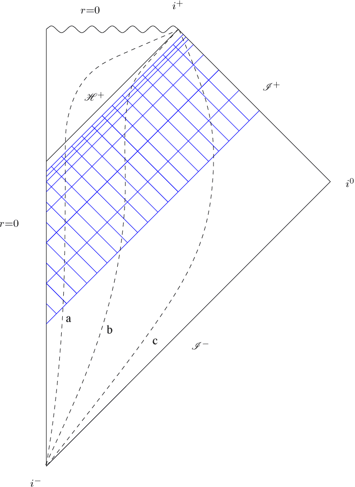
An important aspect of our compactified characteristic evolution scheme is that at late times our null slices asymptotically approach the event horizon, see Fig. 1.1. Essentially this is because our coordinates can not penetrate a dynamical horizon [AK02, AK03, AK04, Hay94b] (they become singular at a marginally trapped surface, e.g. at an apparent horizon), which is spacelike if any matter or radiation falls through it and null otherwise [HE73, AK04]. Note that the dynamical horizon is contained inside of the event horizon, and the outermost dynamical horizon approaches (or coincides with) the event horizon at late times, assuming cosmic censorship holds. This fact makes our approach in some sense complementary to previous critical collapse studies, which were not adapted to the asymptotic regime.
To further investigate physical quantities such as the mass function when a dynamical horizon forms, we employ an uncompactified double-null code which can penetrate dynamical horizons. This code is based on the work of Hamadé and Stewart [HS96] and improvements by Harada and Carr [Har05]. The code has also been developed to analyze collapse problems in dimensional gravity.
In this thesis we focus on those aspects of critical collapse which are associated with global structure, and in particular the phenomenology seen by asymptotic observers. For the sake of completeness, We will also discuss other well-studied aspects such as mass scaling or local DSS behavior in the past self-similarity horizon.
1.1 Organization of this Thesis
This thesis is organized as follows: in chapter 2 we discuss characteristic surfaces of hyperbolic PDE’s, mention different horizon concepts for black holes, and introduce our geometric setup, which is based on Bondi-type coordinates and double-null coordinates in spherical symmetry. In this context we also state gauge and regularity conditions at the origin.
Chapter 3 we present evolution systems for the Einstein-massless scalar field problem in both Bondi and double-null coordinates. We discuss a compactification scheme which introduces the Misner-Sharp mass-function as an independent evolution variable, which renders our evolution system regular at null infinity. We also mention physical quantities of interest, such as the Bondi-mass and Ricci scalar curvature.
Our numerical algorithms are presented in chapter 4. In addition to the numerical schemes for the Bondi and double-null codes, we discuss issues of mesh-refinement, accuracy, convergence and the satisfaction of constraint equations in numerical evolutions.
Chapter 5 deals with critical phenomena in gravitational collapse. We introduce the concept of continuous and discrete self-similarity, the dynamical systems picture and present a standard derivation of the mass-scaling law.
In chapter 6, we introduce quasinormal modes and tails and present heuristic results for the presence of the least scalar damped QNM of a Schwarzschild black hole in critical collapse evolutions. We also study power-law tail exponents in different regions of numerical spacetime.
In chapter 7 we give a detailed discussion of our numerical results pertaining to critical behavior, which include a comparison of the radiation signal at future null infinity with a heuristic estimate based on self-similar scaling and the accumulation of matter exterior to the past self-similarity horizon via backscattering.
Our results and conclusions are summarized in chapter 8.
In Appendix A and B we list tensor components in Bondi and double-null coordinates. Appendix C discusses numerical methods, starting from discretizations of ordinary differential equations and presenting a heuristic error analysis for the NSWE-algorithm. Finally, appendix D mentions the basic methodology which underlies convergence tests.
1.2 Conventions
We use the metric signature and work in “geometrized units” . Spacetime indices are Latin. Space indices are denoted by Greek letters. Angular indices or indices of two-dimensional tensors are denoted by capital Latin letters.
Chapter 2 Geometric Setup
2.1 Some Notes on Hyperbolic PDEs
In this thesis we will essentially be dealing with the numerical solution of nonlinear partial differential equations (PDEs) on characteristic manifolds. Since this characteristic approach is entirely different from and not as common as the standard spacelike Cauchy problem, it is well worth the effort to investigate how characteristics and associated concepts feature in the theory of PDEs.
A quasilinear (hyperbolic in our case) partial differential equation (PDE) of order in n variables for an unknown function can be written: (See Refs. [Gar64], [CH62])
| (2.1.1) |
and thus defines the differential operator .
A submanifold of dimension and equation is said to be a characteristic manifold (surface) if its normals fulfill the first order PDE111The eikonal equation of geometric optics is of that form.
| (2.1.2) |
The Cauchy problem for a order hyperbolic PDE can only be well posed if the manifold on which the initial data is specified is not a characteristic manifold. If it were posed on a characteristic manifold, the PDE would only be first order in time, being an “interior” (i.e. acting purely in the characteristic surface) differential operator, and the derivative transversal to the initial data surface could, in this case, not be determined. Thus, characteristic surfaces are exactly those, on which the Cauchy problem is not well-posed. Note that in the quasilinear case the characteristic condition depends on the initial data, since the are, in general, also functions of .
Characteristic surfaces are, in turn, generated by characteristic rays or bicharacteristics, which satisfy the following equation
| (2.1.3) |
It can be shown that the bicharacteristics of general relativity are null geodesics which generate null hypersurfaces. We will show in section 2.1.1 that the bicharacteristics of a massless scalar field which is minimally coupled to gravity are null geodesics of spacetime. Therefore, since gravitational disturbances, and, in our case, disturbances in the massless scalar field, are propagated along null geodesics, this makes a case for introducing a foliation of spacetime based on a family of non-intersecting null hypersurfaces. It is also worth noting that these disturbances need not be smooth in general, i.e. shock waves are possible in some matter models (e.g. perfect fluids).
As a simple example consider the flat space wave equation
| (2.1.4) |
The characteristics then have to fulfill
| (2.1.5) |
A special solution is the characteristic cone
| (2.1.6) |
which represents spherical wavefronts propagating from a source located at . The generators of the cone, which are bicharacteristics, may be represented as light rays perpendicular to the wavefronts.
It is illuminating to compare the spacelike slices of the formalism with a characteristic foliation based on outgoing null hypersurfaces for the scalar wave equation in Minkowski spacetime with polar spherical spatial coordinates .
In the result is well known:
| (2.1.7) |
This equation is second order in time, i.e. both the field and its time derivative must be specified on an initial slice in order to uniquely determine the future evolution.
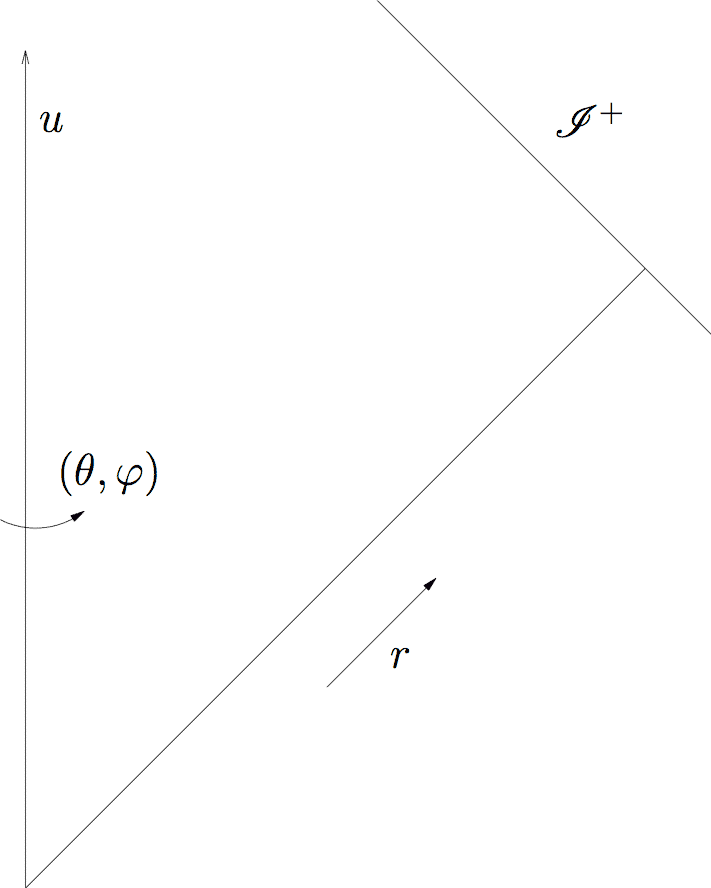
In contrast, let us introduce a coordinate system based on null cones , which are generated by a two-dimensional set of null rays, labeled by the angles and with a radial parameter along the rays. These coordinates will be discussed in detail in section 2.3.2. The line element is
| (2.1.8) |
so that the wave equation then becomes
| (2.1.9) |
where is the angular momentum operator. This equation is only first order in the retarded time , so only the value of the field needs to be specified on an initial slice in order to uniquely determine the future evolution. However, the domain of dependence only extends to the inside of the cone; i.e. the initial null surface is not a Cauchy surface for the spacetime.
2.1.1 The Bicharacteristics of a Scalar Field Coupled to Gravity
Let us consider the matter field equation for the massless scalar field minimally coupled to gravity in spherical symmetry and assume that we can foliate spacetime by null hypersurfaces which are labelled by a coordinate . We will show that the bicharacteristics of the scalar field are null geodesics of spacetime (see [d’I92b]).
The matter field equation is of the form of equation (2.1.1)
| (2.1.10) |
and its principal part (the terms which contain the highest derivatives) is
| (2.1.11) |
The coeffient matrix which appears here, the of (2.1.1), is just the inverse spacetime metric in the (u,r)-submanifold. According to equation (2.1.2) the hypersurfaces are characteristic manifolds since they fulfill
| (2.1.12) |
By definition (2.1.3) the bicharacteristics which generate the surfaces satisfy (with being a parameter along the bicharacteristics)
| (2.1.13) |
i.e., they are the orbits of the vector field .
Now we will prove that these bicharacteristics are, in fact, null geodesics. We take the covariant derivative in the direction of the vector field of the last equation and find
| (2.1.14) |
Thanks to the symmetry of the connection this last expression is equal to
| (2.1.15) |
where we have used that is null. Thus, the bicharacteristics of the massless scalar field turn out to be null geodesics. This intuitively makes sense, since the scalar field propagates at the speed of light. We have also shown that is an affine null vector, that is, (chosen by equation (2.1.13)), is an affine parameter along these null rays.
2.2 General Properties of Black Holes
In the following we give some textbook definitions of a black hole, both from a global and a local point of view [Poi04, Wal84].
The causal past of an event , denoted by is the set of all events that can be reached from by past-directed curves, either timelike or null. The causal past of a set of events , is the union of the causal pasts of all events .
The black hole region of the spacetime manifold is the set of all events that do not belong to the causal past of future null infinity:
| (2.2.1) |
The event horizon is defined to be the boundary of the black hole region:
| (2.2.2) |
Because the event horizon is a causal boundary, it must be a null hypersurface generated by null geodesics. Note that this definition of a black hole depends crucially on the notion of future null infinity which can be defined for asymptotically flat spacetimes. Moreover, to apply this definition one has to know the entire future development of the spacetime in question. In practice, it is often more convenient to use a quasi-local definition of a horizon.
A trapped surface is a closed, spacelike two-dimensional surface such that for both congruences (ingoing and outgoing) of future-directed null geodesics orthogonal to , the expansion is negative everywhere on .
The trapping horizon[Hay94a] is the three-dimensional boundary of the region of spacetime that contains trapped surfaces. 222A trapping horizon is the closure of a three-surface foliated by marginal surfaces on which and . A marginal surface is a spatial two-surface on which one null expansion vanishes, fixed as . The trapping horizon and marginal surfaces are said to be outer if and future if . The concept of dynamical horizons[AK04] is closely related to trapping horizons.
The two-dimensional intersection of the trapping horizon with a spacelike hypersurface (Cauchy surface) is called an apparent horizon. The apparent horizon is therefore a marginally trapped surface – a closed two-surface on which one of the congruences of future-directed null geodesics orthogonal to has zero expansion. 333For technical details see [Wal84] theorem 12.2.5. Note that the intersection of an outgoing null hypersurface with the trapping horizon can be an apparent horizon, or a three-dimensional subset of the trapping horizon.
The trapped region of a spacelike hypersurface is the portion of that contains trapped surfaces.
Under certain technical conditions the black hole region contains trapped surfaces. 444For details see [Wal84] proposition 12.2.3. While for stationary black holes the trapping horizon typically coincides with the event horizon, it lies within the black hole region in dynamical situations (unless the null energy condition is violated.) We will not distinguish between the two-dimensional apparent horizon and the three-dimensional trapping horizon and will refer to both as the apparent horizon. We also use the term “trapped region” in a different sense as defined above, namely we refer to a region of spacetime for which each point lies on a trapped surface [Hay94a].
In the following we will restrict ourselves to future outer trapping horizons (FOTH) and future marginally outer trapped surfaces (MOTS), which require and , where and refers to the outgoing and ingoing null congruences, respectively. A FOTH is either spacelike or null, being null if and only if the shear of the outer null normal as well as the matter flux across the horizon vanishes [AK04].
The apparent horizon is the outermost (future) marginally outer trapped surface (MOTS) in a spacelike hypersurface . If one looks for globally outermost MOTS in a Cauchy evolution, they can “jump” [AMS05]. This does not happen for an outgoing null foliation.
2.3 Bondi Coordinates in Spherical Symmetry
2.3.1 Spherical Symmetry
By definition, the metric of a spherically symmetric spacetime possesses three spacelike Killing vector fields, which form the Lie-algebra of SO(3), the rotation group in three dimensions. The Killing vectors fulfill the following commutation relations
| (2.3.1) |
where the denote the structure constants of SO(3). The commutators close (that is, the commutator of any two fields in the set is a linear combination of other fields in the set), so that by Frobenius’ theorem (see [Wal84]) the integral curves of these vector fields “mesh” together to form submanifolds of the manifold on which they are defined. The orbits of SO(3) are spacelike 2-spheres and the spacetime metric induces a metric on each orbit 2-sphere.
The general form of a spherically symmetric metric is (see appendix B of [HE73])
| (2.3.2) |
where is a two-dimensional metric of indefinite signature and is the canonical metric on . The coordinates are chosen so that the group orbits of SO(3) are the surfaces and the orthogonal surfaces are given by .
2.3.2 Bondi Coordinates
In the following, we define Bondi coordinates and derive the form of the spacetime metric. (see [d’I92b] and [Pap74]). We start from the general form of a spherically symmetric metric given in equation (2.3.2). We chose
| (2.3.3) |
to be a family of non-intersecting, outgoing null hypersurfaces, i.e.
.
We know from section 2.1.1 that these null hypersurfaces are generated
by null geodesics (the bicharacteristics of the surfaces). This gives us the
possibility to define a second coordinate in a purely geometrical way.
We choose
| (2.3.4) |
to be a radial parameter along the outgoing null geodesics that foliate the surfaces, i.e. on each such null ray we have and and .
The remaining coordinates are chosen to be polar angles, coinciding with the usual flat space definitions for
| (2.3.5) |
near the center of spherical symmetry, as we will later choose to be central proper time. This completes our coordinate system to .
Now, we derive the form of the spacetime metric in these coordinates. An outgoing null ray (light ray) is a coordinate curve
| (2.3.6) |
where r is varying, or
| (2.3.7) |
The tangent vector to such a curve ,
| (2.3.8) |
must be parallel to the normal vector to the hypersurfaces
| (2.3.9) |
since, in the case of a null hypersurface, the normal vector is also the tangent and the null rays generate the hypersurfaces. Thus, we find
| (2.3.10) |
which entails
| (2.3.11) |
or equivalently
| (2.3.12) |
We still have freedom in the choice of parametrization along the null rays. Following Bondi, we choose to be an areal radial coordinate or luminosity distance, so that the surface area of , 2-spheres equals . 555Other possible choices include an affine parametrization of the outgoing null rays, as used by Newman and Penrose in their work on gravitational radiation [NP62]. An affine radial coordinate entails by definition which leads to For null coordinates in spherical symmetry the only nonzero contribution comes from A vanishing of and thus diverging of would make the metric singular, therefore the condition to be satisfied is According to the general form of a spherically symmetric metric given in equation (2.3.2), the line element must then be of the following form (2.3.13) This choice can be enforced by the condition
| (2.3.14) |
Note that in spherical symmetry, the areal -coordinate is defined in a geometrically unique way ([Hay96]). It is also possible to compactify the radial coordinate; we discuss this in detail in section 3.6.
Putting these requirements together, we find that the line element reduces to the form
| (2.3.15) |
Since is Lorentzian, we can choose to be timelike, i.e.
| (2.3.16) |
We write the metric in the following way, adhering to Bondi’s conventions for the names of the metric functions
| (2.3.17) |
where is assumed in order that be timelike.
So the metric and inverse metric are
| (2.3.18) |
and
| (2.3.19) |
respectively.
The sign of is due to our use of a retarded null-coordinate . In section 2.3.4 we will choose to be proper time at the origin which implies that the metric reduces to the following flat metric at the origin
| (2.3.20) |
One can also check that this is consistent with the signature by introducing a time coordinate in flat space, so that
| (2.3.21) |
For purposes of comparison, we can also introduce an advanced null-coordinate in flat space, and find
| (2.3.22) |
In the context of Bondi coordinates, we often write partial derivatives of some function with respect to and as and , repectively.
2.3.3 Physical Interpretation of the Bondi Metric
To improve physical understanding, it is worthwhile to analyze the Bondi metric in some further detail.
First, let us take a look at the tangent and normal vectors as shown in table 2.1. By construction, we have
| (2.3.23) |
i.e., lies in the u=const null surfaces. Or, to put it differently, these null rays generate the null hypersurfaces.
Observe also that if is positive, then is a timelike surface and is also timelike. If , both are null, and if both are spacelike. Correspondingly, is spacelike, null or timelike.
| null | |||
| spacelike | |||
| timelike | |||
| null |
The particular choice of the algebraic form of the metric components serves the simplicity of the resulting Einstein equations. The functions and also have simple physical interpretations. As will be shown in section 2.3.4 measures the redshift between an asymptotic coordinate frame of reference and the center of spherical symmetry. is the analog of the Newtonian potential and contains the Bondi-mass in its asymptotic expansion.
We define ingoing and outgoing null directions by
| (2.3.24) |
and
| (2.3.25) |
which is an affine null vector, i.e. . For an affine null vector the null expansion can be defined by (see chapter 9 of [Wal84])
| (2.3.26) |
We find
| (2.3.27) |
If along an outgoing null ray, the surface area of 2-spheres increases and neighboring null rays diverge. Since is positive definite unless diverges, the occurrence of marginally outer trapped surfaces, for some sphere, cannot happen in outgoing Bondi coordinates. Thus, we cannot penetrate apparent horizons (see 2.2).

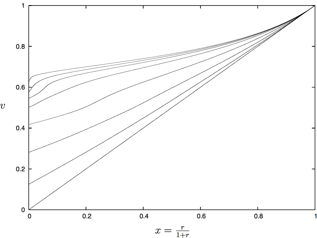
Nevertheless, as we come close to an apparent horizon, our slices will asymptote to it (see figures 2.2 and 2.3) and ultimately, as , will cease to be a good coordinate; it will no longer be a monotonically increasing function of the advanced null coordinate which is defined by , i.e. the curves are the ingoing null-geodesics and on the initial slice. (In flat space .) Tiny numerical errors may lead to the bending over of the slices and thus crash the code.
The radial ingoing null geodesics are given by integration of the equation
| (2.3.28) |
Accordingly, the total derivative of any scalar quantity with respect to along an ingoing null geodesic is given by
| (2.3.29) |
Since this is a Lie-derivative with respect to a non-coordinate vector field, it will in general not commute with partial derivatives like .
2.3.4 Gauge and Regularity Conditions at the Origin
Assume that there is a regular center at (no eternal black or white holes or naked singularities), so that we can designate a finite geodesic line segment of a central observer at as our spatial origin. We fix the gauge such that the family of outgoing null cones emanating from the center is parametrized by the proper time 666 With our choice of Lorentz signature , the proper time of a timelike curve with tangent and curve parameter is given by , , of this central observer. This choice is taken since we are interested in the “echoing region” near the center of spherical symmetry, where oscillations in the fields will pile up if we are near to the “critical solution”. Another common gauge is to choose as the proper time of an observer at future null infinity, . This asymptotically flat time coordinate is the usual choice if one is interested in asymptotics.
Choosing as proper time at the origin implies the condition
| (2.3.30) |
while a regular center, as defined by [Hay96], requires , which in turn entails
| (2.3.31) |
Together theses requirements imply local flatness and regularity of the metric, that is
| (2.3.32) |
at a fixed retarded time . These smoothness conditions are rederived in section 2.3.4.
Relation between Central and Bondi Time
In the following, will always denote central time - proper time at the center of spherical symmetry, whereas we denote the asymptotically flat Bondi time by . The relation between the two time coordinates can easily be derived by comparing with an asymptotically flat (standard Bondi) frame (see section 3.6.1). For large the line elements behave as
| (2.3.33) | ||||
| (2.3.34) |
which yields in the limit
| (2.3.35) |
where and .
The following more geometrical argument yields the same result: In general , but under the following assumptions we can show that only. We demand that
| (2.3.36) |
and
| (2.3.37) |
i.e. are null hypersurfaces.
We find
| (2.3.38) |
which yields
| (2.3.39) |
Thus only. Now we have
| (2.3.40) |
Since is proper time at infinity,
| (2.3.41) |
plugging (2.3.40) in to the metric yields
| (2.3.42) |
Therefore, and we have found the desired relation between central and Bondi time:
| (2.3.43) |
Redshift
Consider a freely falling observer located at whose worldline is tangent to the timelike geodesic parametrized by proper time at the origin with tangent . He sends out a light signal which propagates along the affinely parametrized outgoing radial null geodesic with tangent (As shown in section 2.1.1, is an affine null vector). The signal is received by an observer whose worldline is tangent to a timelike geodesic at , parametrized by proper time at infinity with tangent .
The frequency (see Ref. [Wal84]) of an emitted wave is given by minus the inner product of the wave vector (which is just the rate of change of the phase of the wave) with the 4-velocity of the observer. The frequency of emission at the center is given by
| (2.3.44) |
The frequency of reception at infinity is, using the relation between central and Bondi time (2.3.35),
| (2.3.45) |
The redshift-factor is defined as
| (2.3.46) |
For small we thus have .
Now, because of the hypersurface equations (see section 3.3) and gauge choice for , the metric functions, and , are both monotonically increasing in the direction of increasing and both are positive definite. Thus and
| (2.3.47) |
always, which is just the condition for signals to be redshifted. In the case of horizon formation , however, will tend to infinity, so that light rays can no longer escape to infinity and the redshift will diverge exponentially until our coordinates break down.
A crude argument for the redshift is also apparent just from the relation (2.3.35). If , a finite amount of central time corresponds to an infinite amount of Bondi time and thus light signals originating from the center are infinitely redshifted.
Derivation of Regularity Conditions at the Origin of Spherical Symmetry
In this section we apply the general procedure for deriving regularity conditions set forth by Bardeen and Piran in [BP83]. Although the latter deals with axisymmetric systems, it is nevertheless worthwhile to study this approach in the simpler setting of spherical symmetry.
A tensorial quantity is called regular at if and only if its components relative to Cartesian coordinates can be expanded in non-negative integer powers 777 Otherwise the tensorial quantity or its derivatives will blow up at . of x, y and z; i.e. one demands the existence of a Taylor series expansion in Cartesian coordinates. We would like to derive what restrictions this assumption of regularity at the origin implies for the metric functions and as functions of .
We will work in a regular coordinate system with defined as . 888Note that the coordinates are not regular: The vector fields , and all have a kink at the origin. Since we have taken to be proper time at the origin, also measures proper time at . We also enforce local flatness at the center, i.e. the metric goes to the Minkowski metric as tends to ,
| (2.3.48) |
We will have to investigate which derivatives of the metric functions are allowed to be non-zero and which are zero by regularity.
The relations between the two coordinate systems are:
The Jacobian for this coordinate transformation is
| (2.3.49) |
First we need to calculate the components of the metric in coordinates. Some interesting components as functions of the polar coordinates are
| (2.3.50) |
| (2.3.51) |
| (2.3.52) |
| (2.3.53) |
| (2.3.54) |
We will also need derivatives of the metric. Since the derivatives of and are particularly messy and we do not need to consider them, we leave them out.
| (2.3.55) |
| (2.3.56) |
| (2.3.57) |
We make the following series ansatz for the metric functions and :
| (2.3.58) | ||||
| (2.3.59) |
This yields
| (2.3.60) | ||||
| (2.3.61) | ||||
| (2.3.62) |
We now impose the local flatness gauge condition (2.3.48).
| (2.3.63) |
yields
| (2.3.64) |
Similarly, we have
| (2.3.65) |
from which we find
| (2.3.66) |
and thus, it follows from (2.3.64) that
| (2.3.67) |
One does not need to consider any other equations, since the two constant terms in (2.3.58) have now been determined. Indeed, one can also check that and are fulfilled.
The series that respect this gauge choice are
| (2.3.68) | ||||
We are now in a position to investigate limits () of the derivatives of the metric. The values should remain finite and be direction independent, i.e. independent of the spherical angles and , since these are indefinite at the origin. This will then provide us with conditions on the series expansions of and . Consequently, we find from (2.3.55), the equation for , that
| (2.3.69) |
Applying the expansions (2.3.4), we find
| (2.3.70) |
and eventually
| (2.3.71) |
Similarly, we find from (2.3.57), the equation for , that
| (2.3.72) |
Here, we can set all terms proportional to to zero and insert the series expansions (2.3.4). We find
| (2.3.73) |
which leads to the condition
| (2.3.74) |
Combining the two conditions (2.3.71) and (2.3.74) we recover
| (2.3.75) | ||||
| (2.3.76) |
We did not consider , since it is already well behaved because of the gauge condition alone. For the calculation would have been more involved but would have led to the same result.
Summarizing, we have found that the metric functions and guarantee that the metric is regular at the center of spherical symmetry if they satisfy, at a fixed retarded time ,
These regularity conditions are consistent with the hypersurface equation (3.3.3), , derived in chapter 3.3.
The conditions we have derived are sufficiently accurate for our purposes, though one could consider higher derivatives of the metric. We will see from the following simple argument that, in fact, all odd derivatives of the metric functions have to vanish at the origin.
Without loss of generality, define linear distance by
| (2.3.78) |
We demand that the metric does not have a kink as the origin is crossed along a ray parametrized by linear distance . If a metric function contains a linear term in its Taylor expansion around the origin, then
| (2.3.79) |
where is a constant.
| (2.3.80) |
has a jump discontinuity and is thus not regular. It will be regular provided that the constant vanishes. This is equivalent to the condition that
| (2.3.81) |
Note that this argument can be extended to higher derivatives. Roughly speaking, each time one applies to a function , reverses its sign for . Therefore, all derivatives of an odd order have to vanish at the origin, so that a regular function of will have a Taylor series which contains only even terms in :
| (2.3.82) |
In addition, we can also derive the Taylor series expansion for the scalar field by making use of the hypersurface equation (3.3.2) and find that there is no restriction on :
| (2.3.83) |
In this respect it is also interesting to view this last fact from a different perspective: When working in polar coordinate systems, the d’Alembertian usually contains terms similar to . Regularity of the field at the origin then amounts to requiring that vanishes. But using a null coordinate makes a difference. There is now a rivaling term in the d’Alembertian (A.0.22) which happens to cancel the other term at the origin.
2.3.5 Historical Notes on the Bondi Coordinate System
The original motivation for Bondi and his co-workers (see [HB62]) in developing this coordinate system was to analyze radiation from an isolated system. To do so, one needed to deal with expansions in negative powers of a radial distance for various quantities. Such a treatment is, however, made impossible by the appearance of logarithmic terms in , as is the case, in Schwarzschild coordinates.
Later, the conformal compactification of null infinity allowed a geometrized description of the asymptotic physical properties of radiative spacetimes. This novel technique also proved very beneficial for the study of gravitational radiation, see e.g. [Fra04].
One demands that in a region from inwards the coordinate system should be non-singular. Farther in, null rays will, in general, focus and cross, forming caustics and causing the coordinates to break down and become singular. 999Except for the case where there exists a second regular center, where rays may caustic, this cannot happen in spherical symmetry, because the lightrays are ’running’ after each other but never touch. A second regular center is however ruled out by the assumed existence of future null infinity . The only caustic that is present in spherical symmetry is a point caustic at the center itself, which has to be handled by regularity conditions on the metric and the matter fields. Of course, for nontrivial topologies the situation is entirely different: e.g. on the Einstein cylinder lightrays may form caustics.
The Bondi-like coordinates defined in section 2.3.2 cover all of spacetime provided there are no caustics or singularities and exists. 101010For the existence of , which is a part of conformal infinity, the spacetime metric has to satisfy certain falloff conditions, i.e. it must tend to a flat metric sufficiently fast as one goes to infinity in an outgoing null direction. In a coordinate independent formulation a spacetime is said to be asymptotically flat, if the physical spacetime can be mapped into a new, “unphysical” spacetime via a conformal isometry which has to satisfy certain, very technical conditions. Details can be found in chapter 11 of Ref. [Wal84].
2.4 Double-Null Coordinates
As we have seen in section 2.3.3, outgoing Bondi coordinates cannot penetrate apparent horizons, because the areal radial coordinate fails to be a good coordinate when an AH forms: . A coordinate system which does not suffer from this deficiency and is suitable for spherically symmetric critical collapse evolutions are double-null coordinates.
In addition to the retarded null-coordinate which is constant on outgoing light rays, we now introduce an advanced null-coordinate , which is constant on ingoing light rays and replaces as a coordinate. Along with the standard polar coordinates on the group orbits of SO(3), , the coordinate chart becomes . The line element is then of the following form
| (2.4.1) |
The area radius is now a metric function that depends on the null coordinates. The double-null form is natural in the sense that each two-sphere possesses two preferred normal directions, the null directions and .
The components of the metric and inverse metric are given by
| (2.4.2) |
and
| (2.4.3) |
and the metric determinant is
| (2.4.4) |
A relation between Bondi coordinates and double-null coordinates can be established by a coordinate transformation (see Ref. [PL04]) of the form
| (2.4.5) |
with an integrating factor .
The line-element is
| (2.4.6) |
In the new coordinates and we can introduce a metric function , so that and the line-element becomes equation (2.4.1).
Since we have the relations
| (2.4.7) | ||||
| (2.4.8) |
In the context of double-null coordinates we denote partial derivatives of some function with respect to and by and , respectively.
2.4.1 Null Expansions
To compute marginally trapped surfaces we compute the null expansions (see Ref. [Wal84])
| (2.4.9) |
where the affine ingoing and outgoing null vectors are defined through their covectors as
| (2.4.10) | ||||
| (2.4.11) |
This yields
| (2.4.12) | ||||
| (2.4.13) |
It is easy to check that the are indeed affine null vectors, that is and that the null expansions are given by
| (2.4.14) | |||
| (2.4.15) |
The signs of the null expansions are geometrical invariants, while their actual values are not [Hay96]. For future marginally outer trapped surfaces (MOTS) (see section 2.2) we need to have while . Since the denominators in equations (2.4.14) and (2.4.15) are non-negative, the sign of the null expansions is determined by the quantities and and it suffices to check the conditions while .
The possible presence of multiple MOTS on an evolution hypersurface depends on the slicing. For outgoing null slices, there cannot be more than one MOTS on a slice, whereas for spacelike slices there can be. The geometric property of future outer trapping horizons being spacelike or null (the latter only if there is no more infalling matter when following the null geodesic generators further outwards), but never timelike, applied to the intersection of an MOTS with an outgoing null-slice shows that we cannot have multiple MOTS on such a null-slice, which is equivalent to the function having at most one zero.
2.4.2 Gauge Choice
The form of the metric is preserved under diffeomorphisms and . We fix this residual gauge freedom present in the null coordinates and by choosing
-
•
to be at
-
•
.
Chapter 3 The Continuum Problem
We consider the coupled spherically symmetric Einstein-massless scalar field system, both in Bondi and in double-null coordinates. After deriving the Einstein equations and the curved space wave equation for the scalar field, we analyze the evolution systems and formulate the characteristic initial value problem to be solved. We also discuss compactification for Bondi coordinates and highlight some quantities of physical interest which we will use in the numerical evolution codes described in the following chapter.
3.1 Einstein’s Equations
To derive Einstein’s equations we start with the action functional which consists of the Einstein-Hilbert action plus the matter action:
| (3.1.1) |
where denotes the Ricci scalar and the Lagrangian density of the massless scalar (Klein-Gordon) field is given by
| (3.1.2) |
Variation of the total action (3.1.1) with respect to the spacetime metric yields the Einstein equations,
| (3.1.3) |
where
| (3.1.4) |
is the energy momentum tensor of the massless scalar field obtained via variation of the matter action with respect to the spacetime metric.
To complete the system, variation of the matter action with respect to the scalar field yields the matter field equation, the curved wave equation for the massless scalar field
| (3.1.5) |
3.2 Hierarchy of Einstein Equations in Bondi Coordinates
In spherical symmetry, the four algebraically independent Einstein equations, the , , , and components of equation (3.1.3), are not differentially independent.
Essentially, we have four equations for two unknown metric functions, and . In principle, one could freely choose two of these equations and complement them with the matter field equation to complete the evolution system. Numerical considerations dictate, however, a preference for the constraint equations (which here act in the outgoing null hypersurfaces, i.e. they are ODEs in the radial coordinate ). Choosing these two hypersurface equations instead of the other wave-type Einstein equations naturally ensures enforcement of the constraints. Unconstrained (or free) evolution systems let the solutions drift off the constraint surface of the Einstein equations and may excite numerical unstable modes, while constrained evolution cuts back on numerical constraint violations and offers greater stability.
There is an analysis of the Einstein equations for the original axissymmetric vacuum Bondi problem according to which the equations decompose into the following sets (see Refs. [HB62] and [d’I92b]):
-
•
four main equations:
-
–
dynamical equation:
(3.2.1) -
–
hypersurface equations:
(3.2.2) where . They contain only derivatives that act in the hypersurfaces
-
–
-
•
symmetry conditions:
(3.2.3) These components vanish identically because of axisymmetry.
-
•
trivial equation:
(3.2.4) -
•
supplementary (conservation) conditions (for energy and angular momentum)
(3.2.5) If they are imposed on a world line, the conservation conditions reduce to regularity conditions on the vertices of the null cones. They are the analog with respect to an r-foliation of the 3+1 momentum constraints.
It follows by the Bianchi identities that, if the main equations are satisfied, the trivial equation is automatically fulfilled and the conservation conditions are satisfied on a complete outgoing null-cone if they hold on a single spherical cross-section (e.g. at infinity).
Our situation is, of course, entirely different, we work in spherical symmetry and have a matter field coupled to gravity. Still, one might expect to obtain some useful insights into the hierarchy of the equations by attempting a similar analysis. We now show how Einstein’s equations split into hypersurface equations, and equations which are automatically satisfied if certain conditions are met.
In the context of Bondi coordinates, we often abbreviate partial derivatives of a function with respect to and by and , respectively.
The hypersurface equations follow indeed from straightforward analogues of equations (3.2.2):
| (3.2.6) |
yields
| (3.2.7) |
while from 111We may rewrite Einstein’s equations as , where is the trace of the energy momentum tensor of the scalar field.
| (3.2.8) |
we have, using equation (A.0.21),
| (3.2.9) |
and finally 222Equation (3.2.10) can also be derived from the component of Einstein’s equations when plugging in equation (3.2.7).
| (3.2.10) |
The dynamical equation (3.2.1) is satisfied if the hypersurface equations (3.2.7) and (3.2.10) hold everywhere and the energy momentum tensor is covariantly divergence free: Inserting the hypersurface equations in equation (3.2.1) leads to
| (3.2.11) |
This equation is satisfied if .
Clearly, this equation cannot contribute to the dynamics in our setting, since in spherical symmetry there are no gravitational degrees of freedom and the dynamics resides entirely in the matter field. 333 Birhoff’s theorem shows that a spherically symmetric vacuum solution is necessarily static. The conservation of mass and angular momentum in general relativity prohibits the existence of spherically symmetric and of dipole waves in the gravitational field. The lowest possible symmetry is that of a quadrupole which already requires at least axisymmetry.
The symmetry conditions, equations (3.2.3), vanish identically because of spherical symmetry. What remains to be discussed is the analogue of the trivial equation, equation (3.2.4), and one of the conservation conditions (3.2.5), .
The trivial equation is satisfied if the hypersurface equations (3.2.7) and (3.2.10) hold everywhere:
| (3.2.12) |
Assuming that the hypersurface equations (3.2.7) and (3.2.10) hold everywhere, the conservation condition can be rewritten as
| (3.2.13) |
At the world line of the central observer, , this equation is satisfied if the regularity conditions, equations (2.3.4), imposed by spherical symmetry hold. The - component of the contracted Bianchi identities , which must also hold for the energy momentum tensor as a consequence of the Einstein equations, yields the following equation
| (3.2.14) |
where we use the shorthand . Since we have already shown that everywhere, we have
| (3.2.15) |
and thus
| (3.2.16) |
Combined with at , we have shown that everywhere.
If one considers the set of hypersurface equations plus the matter field wave equation, it is apparent that three integration constants will be necessary to carry out an actual time evolution. These constants have been fixed by our choice of proper time at the origin. Otherwise, for asymptotically flat coordinates, as in Bondi’s original work, one chooses the integration constants at infinity. In section 3.6.1 will make an acquaintance with these integration constants (which in our gauge are functions of ) and we will see that the conservation condition imposed at future null infinity, , yields a differential relation between two of them, the Bondi mass-loss equation.
3.3 Field Equations for the Gravitating Massless Scalar Field
Given the massless scalar (Klein-Gordon) field, all gravitational quantities can be determined by integration along the characteristics of the null foliation, since the matter field is the only dynamical field in spherical symmetry and needs to be included to make the system non-Schwarzschild. This is a coupled problem since the scalar wave equation involves the curved space metric.
The field equations consist of the wave equation for the scalar field
| (3.3.1) |
and two hypersurface equations for the metric functions:
| (3.3.2) |
| (3.3.3) |
Note that both and are monotonic in . Combined with the gauge conditions imposed in section 2.3.4 monotonicity implies
| (3.3.4) | ||||
| (3.3.5) |
In spherical symmetry the curved space d’Alembertian 444This can easily be obtained by using the formula and setting . is
| (3.3.6) |
We will now derive a useful relation between the four-dimensional wave operator and the wave operator in the two-dimensional (u,r) submanifold. The intrinsic metric in the (u,r) submanifold is
| (3.3.7) |
and thus the two-dimensional d’Alembertian follows as
| (3.3.8) |
Now we introduce a rescaled field which factors out the known falloff of at large
| (3.3.9) |
It is then straightforward to derive the following identity:
| (3.3.10) |
and use this to write the wave equation as
| (3.3.11) |
The motivation for introducing the rescaled field is the following: The amplitude of an outgoing spherical wave packet decreases with , a rescaled field thus behaves similarly to a plane wave. Indeed the following identity holds: In the flat background case, the field satisfies the usual -dimensional wave equation . Thanks to the plane wave behavior of , numerical accuracy is expected to benefit for large since the amplitude of the wave does not change as fast.
3.4 The PGG Evolution Algorithm
Here we briefly discuss a characteristic evolution scheme due to Piran, Goldwirth and Garfinkle [GP87], [Gar95]. We essentially follow the original algorithm although the terminology is slightly different.
3.5 The Gomez-Winicour “Diamond” Algorithm
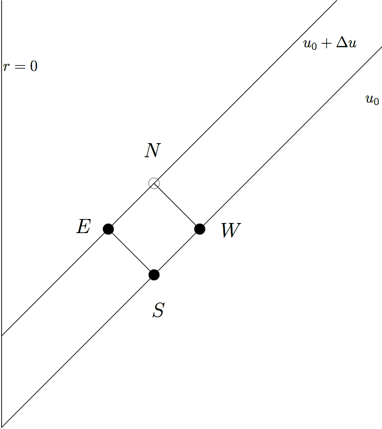
The basic idea of this algorithm (see Refs.[GW92b], [GW92c],[Win05]) is to integrate the wave equation over the null parallelogram spanned by the points N, S, W, and E (see figure 3.1 on page 3.1). Using the identity (3.3.11) and the volume element We have
| (3.5.1) |
The crucial trick of the whole undertaking is the following: Since h is a two-dimensional metric, it is conformally flat. As we will shortly see, has conformal weight 555See [Wal84] Appendix D for a definition. whereas the surface area element has conformal weight . Thus, the surface integral over is identical to the flat space result which can easily be obtained.
Let be a conformal rescaling of the metric . First we need to know how the determinant of the metric transforms under conformal transformations. For a two-dimensional metric we have
and therefore
i.e. the volume element in two dimensions has conformal weight . The formula for the d’Alembertian is
Applying the previous result yields
i.e. the two-dimensional d’Alembertian has conformal weight -2. So, all in all we can rewrite the original surface integral in the following manner:
The flat two-dimensional (Minkowsi-)metric can be rewritten in double-null coordinates as . The metric is So that the d’Alembertian becomes . Now our integral can easily be evaluated:
where we have introduced the grid points , , , and as shown in figure 3.1
Using (3.3.11) and the volume element , the wave equation can thus be written as
| (3.5.2) |
3.6 Compactification of the Radial Coordinate
Compactification is rather simple for characteristic codes, and has been used extensively in the characteristic approach to numerical relativity [GW92b, GW92a, GW92c, Win05].
The type of compactification we pursue here is not conformal compactification per se (see Ref. [Fra04] for a review), where the spacetime manifold is completed by “attaching” a boundary at “infinity”. The method of conformal compactification maps physical spacetime onto a bounded open region of unphysical spacetime, introduces an unphysical metric via a conformal rescaling ( approaches zero (at infinity) at an appropriate rate), and factors out known asymptotic behavior of geometrical quantities by a conformal transformation.
Rather, we use an ad-hoc regularization adapted to the simple geometry which could be related to conformal rescalings [Hus07]. We employ a simple coordinate transformation with respect to the radial coordinate, which maps a half-infinite domain to a compact interval . In this ad-hoc approach the metric is not altered (no unphysical metric is introduced) and the evolution equations “notice where infinity is” because they degenerate there [Fra04]. The advantage of this compactification method are its simplicity and that we can evolve till future null infinity, and thus study global and radiative properties of collapse spacetimes in detail.
We would like to emphasize that the use of conformal rescalings does not imply that one has to employ the rather difficult framework of Friedrich’s regular conformal Einstein equations [Fri81]. In fact such an approach has also been suggested in [And02, HSVZ05].
Before introducing compactification we want to say a few words about asymptotic series expansions.
3.6.1 Asymptotic Series Expansions for the Massless Scalar Field
Assuming initial data that are smooth at , one can expand the massless scalar field in powers of near 666A constant term in the expansion of has been omitted since one can trivially rescale the coupled Einstein massless scalar field system: A transformation leaves invariant.
| (3.6.1) |
The coefficient of the - term in the expansion is a Newman-Penrose constant [NP68] of the scalar field.
3.6.2 Compactified Evolution Scheme
First, we introduce a compactified radial coordinate, then we recalculate our evolution equations and aim to regularize them at null infinity.
Starting with our standard Bondi-like coordinates (u,r,,) we introduce a compactified radial coordinate
| (3.6.7) |
which maps , so that points at are automatically included in the grid at . Consequently, we have the relations
| (3.6.8) |
The line element, equation (2.3.17), then becomes
| (3.6.9) |
which evidently contains singular terms. Regularity, however, only requires that the field equation for the scalar field and the hypersurface equations for the metric functions be well behaved.
A naive approach of rewriting the hypersurface equations in terms of the -coordinate leads to a singular equation for the quantity
| (3.6.10) | ||||
| (3.6.11) |
while the equation for is fine.
The introduction of a renormalized quantity (chosen such that ) lets us rewrite the hypersurface equation (3.6.11) in the following form
| (3.6.12) |
which remedies the situation somewhat. Still, it is not obvious that is well behaved at , since the denominator of equation (3.6.12) tends to zero. An asymptotic expansion shows that is nonsingular,
| (3.6.13) |
but the cancellation in the numerator of (3.6.12) that brings about this result is very delicate in numerical terms.
As described in [PHA05], to obtain a fully regular system of evolution equations, we eliminate (or ) by the Misner-Sharp mass-function
| (3.6.14) |
which satisfies
| (3.6.15) |
The set of hypersurface equations then becomes:
These equations are now completely regular. Note that the term does not cause problems because of the smoothness of the metric at the regular center (2.3.4).
In section 4.1.1, we will choose our gridpoints to freely fall along ingoing radial null geodesics which fulfill
| (3.6.17) |
In section 4.1.3 we will argue that this choice is crucial to resolve DSS phenomena.
For the matter field equation takes the form
| (3.6.18) |
At this reduces to the ODE
| (3.6.19) |
The diamond scheme can be derived by applying the transformation to the x-coordinate to equation (3.5.2), which yields
| (3.6.20) |
Equations (3.6.2) and (3.6.20) now form a manifestly nonsingular set of evolution equations for the massless scalar field coupled to gravity.
The gauge and regularity conditions (2.3.4) outlined in section 2.3.4 and the regularity of the scalar field (2.3.83) along with the definition of the rescaled field , equation (3.3.9) now become
| (3.6.21) |
In section 4.1.2 we discuss Taylor expansions in the vicinity of the origin.
3.7 Diagnostics
3.7.1 The Misner-Sharp Mass
In spherical symmetry, there exists a well defined notion of quasilocal energy, the Misner-Sharp mass-function (see Refs. [MS64] and [Hay96]):
| (3.7.1) |
which in outgoing Bondi coordinates yields
| (3.7.2) |
Note that is a smooth function. The Misner-Sharp mass measures the energy content of a sphere of radius and reduces the ADM and Bondi masses in the appropriate limits. We also refer to the Misner-Sharp mass-function defined in equation (3.7.2) as , in order to distinguish it from an integral expression for the local mass, which we define below.
We write equation (3.7.2) as an integral along outgoing radial null geodesics :
| (3.7.3) |
and then use Einstein’s equations to simplify the integrand:
| (3.7.4) |
Since is a form of local energy density, we refer to its integral (defined by equation (3.7.3)) as the “integrated-scalar-field mass-function”.
On the continuum level, the mass-functions and are clearly identical, but numerically they will in general differ by a small amount due to having different finite differencing errors; their difference is a good “diagnostic” of the code’s accuracy.
To this end, we define
| (3.7.5) |
where is the total mass of our initial slice, i.e. the mass-function at the outer grid boundary on the initial slice. is a dimensionless measure of how well our field variables satisfy the Einstein equations; we must have everywhere in the grid at all times for our results to be trustworthy.
3.7.2 The Bondi Mass and the News Function
Taking the limit of the Misner-Sharp mass-function, , as at constant , we obtain the Bondi mass:
| (3.7.6) |
In an isolated system outgoing waves can radiate physical energy to future null infinity, . Therefore, the Bondi mass is in general not conserved in retarded time. (In contrast, the ADM mass, which is defined by taking the limit of as at constant , that is, on a spatial slice, is conserved in .)
Moreover, one can show (see Ref. [Wal84]) that there exists a flux such that
| (3.7.7) |
where is a cross-section of with a null hypersurface and is a real interval.
We will derive a relation between the outgoing radiation flux, which is described in terms of the scalar news function, and the change of the Bondi mass in time. This relation is known as the Bondi mass-loss equation. (As always, denotes central time and not Bondi time. The two time coordinates are related by equation (2.3.35).)
We insert the asymptotic series expansions of the fields and , given in equations (3.6.1), (3.6.2) and (3.6.3), respectively, into the -component of the Einstein equations
| (3.7.8) |
and obtain
| (3.7.9) |
As it turns out, the third and the fourth terms are crucial, all the other terms are at least or cancel out. We find
| (3.7.10) |
Now, we introduce the scalar news function as
| (3.7.11) |
Combining the last two equations yields the Bondi mass-loss equation
| (3.7.12) |
In Bondi time, it becomes, using relation (2.3.35),
| (3.7.13) |
From equation (3.7.7) we find
| (3.7.14) |
Thus, the square of the news function is just the flux that appears in the integral (3.7.7):
| (3.7.15) |
The positivity of the flux-function entails that
| (3.7.16) |
always. “News”, that is radiation, can only decrease the Bondi mass contained on a collection of null-slices that extend to . But the Bondi mass can never increase to the future.
3.7.3 The Bondi Mass as a Linkage Integral
Let be a generator of an asymptotic time-translation and let be a one-parameter family of spheres which approach the cross-section of . Then the Bondi mass is defined as (see Refs. [GW81] and [Wal84])
| (3.7.17) |
where the gauge condition must be fulfilled in a neighborhood of . For the Bondi metric, equation (2.3.17), the condition gives
| (3.7.18) |
if . The generator of (asymptotic) time translations
| (3.7.19) |
satisfies the vanishing divergence condition as can be verified by making use of the asymptotic expansions for and given in section 3.6.1. Now the integrand of equation (3.7.17) is
| (3.7.20) |
so that one obtains
| (3.7.21) |
where is the coefficient in the asymptotic expansion of .
3.7.4 The Ricci Scalar Curvature
From the Einstein equations (3.1.3) for a minimally coupled massless scalar field one finds by taking the trace
| (3.7.22) |
the following expression for the Ricci scalar
| (3.7.23) |
For the Bondi metric (2.3.17) this yields
| (3.7.24) |
3.8 Double Null Equations
To complement the DICE code which is based on Bondi coordinates, we introduce a first order formulation of the Einstein-scalar field system in double null coordinates which offers the advantage that it can penetrate apparent horizons.
We consider the Einstein massless scalar field equations for the spherically symmetric metric introduced in section 2.4
| (3.8.1) |
in double-null coordinates . The tensor components are given in appendix B. We often use shorthands for partial derivatives:
| (3.8.2) |
We set to simplify the appearance of the matter field terms and define additional variables in order to write the equations in first order form following Ref. [HS96].
First, we define the following evolution variables
| D1: | (3.8.3) | ||||
| D2: | (3.8.4) | ||||
| D3: | (3.8.5) | ||||
| D4: | (3.8.6) | ||||
| D5: | (3.8.7) |
The Einstein and matter field equations then become
| E1: | (3.8.8) | ||||
| E2: | (3.8.9) | ||||
| C1: | (3.8.10) | ||||
| C2: | (3.8.11) | ||||
| S1: | (3.8.12) | ||||
| S2: | (3.8.13) |
where we denote Einstein equations of wave-type by the letter E, constraint equations by the letter C, and the scalar field wave equation by the letter S.
Boundary conditions at the center of spherical symmetry are dictated by regularity and gauge choices as detailed in sections 2.4.2, 3.8.1 and 3.8.2 and
| (3.8.14) | ||||
| (3.8.15) | ||||
| (3.8.16) | ||||
| (3.8.17) |
To evolve the coupled first order system, we choose a constrained evolution using equations E2, S1 and D2, D5, C2, D4. This leaves equations C1, D1 and D3 for checking the numerical solution.
We need to specify the variables at the axis, while and are calculated from evolution equations. Obviously, at the axis.
3.8.1 Regularity and Boundary Conditions
Regular Variables at the Center
We demand that our evolution variables (metric functions, scalar field) be well defined at the center of spherical symmetry. See [AG05] for a detailed analysis for Cauchy problems. As we have seen in section 2.3.4, this is most easily obtained by demanding that the variables must not have a kink as the origin is crossed along a ray parametrized by linear distance . Effectively, this forces all odd derivatives of the metric with respect to at constant to vanish at the origin. 777We may use flat space coordinates since we impose local flatness later.
Therefore, must be an even function of , i.e.
| (3.8.18) |
so that we arrive at the boundary condition
| (3.8.19) |
Similarly, we have for the scalar field
| (3.8.20) |
We can also investigate the behavior of
| (3.8.21) |
Local Flatness at the Center
As it turns out, one has to also impose local flatness to ensure a regular behavior in the evolution equations. Again, see [AG05] for details. Local flatness means that the spatial metric locally looks like the flat metric
| (3.8.22) |
In double-null coordinates the flat spacetime metric is given by
| (3.8.23) |
where and is given by
| (3.8.24) |
It then follows that or, in the notation of section 3.8),
| (3.8.25) |
and also that .
Due to spherical symmetry and local flatness, has to decrease as fast (with u) on an ingoing (radial) null ray as it has to increase (with v) on an outgoing null ray close to the origin. Also, a null ray through the origin only appears to change direction in spherical coordinates, while it obviously passes straight through in Cartesian coordinates.
As we impose local flatness at the center, we may use flat space coordinates to express boundary conditions, such as . It is straight forward to implement such boundary conditions on an equispaced double null grid.
Issues of regularity of the evolution equations are discussed in section 3.8.2.
3.8.2 Regularity of Evolution Equations
At , the formally singular right hand sides of equations E1, E2, and S1, S2 yield the following conditions:
| (3.8.26) | |||
| (3.8.27) | |||
| (3.8.28) |
The last condition leads to the final boundary condition needed, which is simply
| (3.8.29) |
3.8.3 Diagnostics for the Double-Null System
We calculate the density function ,
| (3.8.30) |
where is the Misner-Sharp mass, defined in section 3.7.1,
| (3.8.31) |
The quantity is used as an indicator for critical behavior and for the closeness of a slice to the formation of an apparent horizon. To detect and measure an apparent horizon we search for a zero in the function (see 2.4.1).
The scalar curvature can be expressed in terms of the scalar field or the geometry:
| (3.8.32) |
The scalar field energy density is given by
| (3.8.33) |
It is instructive to introduce observers at constant radius . We would then like to compute the proper time along each of these worldlines of constant . Following [HS96] we invert to obtain . At , it follows that . The line element (2.4.1) then becomes
| (3.8.34) |
Then, we have
| (3.8.35) |
At , local flatness implies , and thus
| (3.8.36) |
Chapter 4 Numerical Algorithms
4.1 The DICE-code
The compactified code used in [PHA05] is based on the “DICE” (Diamond Integral Characteristic Evolution) code, which has been documented in [HLP+00] (there particular emphasis is given to detailed convergence tests).
4.1.1 Our Overall Computational Scheme
While this section discusses the uncompactified Bondi evolution algorithm, it can be applied to the compactified system, by a few simple replacements. Most notably, the metric function has been replaced by the Misner-Sharp mass . See section 3.6 for further details.
Summary
We first construct initial data:
-
1.
Choose the field on a null slice .
-
2.
Also choose the positions, , of our grid points on this same initial slice.
- 3.
Our integration scheme starts by first integrating the geodesics back in time one step , since our geodesic integrator needs two slices to work. Now suppose we know all the gravitation and matter fields for time levels . To determine them for time level , we use the following algorithm (we use the usual notation where superscripts denote time levels):
-
1.
Determine the Taylor expansion of near the origin (cf. section 4.1.2).
-
2.
For each grid point in some small (typically 3 grid points) “Taylor series region” starting at the origin and working outwards,
-
3.
Now for each grid point in the rest of the grid, starting just outside the Taylor series region and working outwards,
Discretization of the Evolution System
We evaluate the integral in equation (3.5.2) by treating the integrand as constant over the (small) null parallelogram , as shown in figure 3.1. Thus we can compute the integrand at the center of which in turn equals its average between the points and to second order accuracy:
| (4.1.1) |
where . Then we multiply the integrand by the area of the null parallelogram , which can be approximated by
| (4.1.2) |
As will be discussed in section C.3, this algorithm is globally 2nd order accurate; for the special case of a flat background () the algorithm is exact.
We use the explicit trapezoidal method (see equation (C.2.8) in appendix C) to discretize the hypersurface and ingoing null geodesic equations. In principle the discretization is straightforward, with the exception of the null geodesic equation. The corrector requires evaluating the right hand side at the time-level, but this has not been computed yet at the time we do the geodesic integration. To solve this problem, we radially extrapolate the needed value from and one spatial gridpoint inwards at the same time-level. At the origin, we know thanks to local flatness, anyway.
Freely Falling Gridpoints
The original Winicour algorithm uses a fixed grid (i.e. the radial positions of the grid points do not move in the course of evolution. As the coordinate velocity of light is in general not constant in a curved space-time, the vertices , , and of the null parallelogram cannot be chosen to lie exactly on the grid. Therefore one has to use interpolation to compute the matter field and metric functions at the vertices.
In the DICE code we used a different approach (which is, in fact, borrowed from a different characteristic evolution scheme due to Piran, Goldwirth and Garfinkle [Gar95] as described in section 3.4): Our gridpoints free-fall along ingoing null geodesics. To compute the locations of the gridpoints on a new slice we integrate the ingoing null geodesic equation
| (4.1.3) |
With this approach, the vertices of the null parallelogram in the diamond algorithm (cf. section 3.5) are gridpoints, so we don’t have to interpolate there.
As well as avoiding interpolation, this scheme has the additional advantage that it provides a sort of adaptive grid refinement for free, since, in regions of strong gravity, the null geodesics are being focussed and thus the density of gridpoints is increased.
Since our grid points move along ingoing null geodesics, each grid point eventually reaches the origin. At this point it disappears, i.e. we remove it from the grid.
Stability of the Winicour algorithm and adaptive choice of timesteps
Assuming that the gridpoints follow ingoing null geodesics, we want to impose a restriction on the “drift” of individual gridpoints from one slice to the next. It follows from the null geodesic equation (4.1.3) that, if we want the change in r from a slice to to be smaller than a factor (’drift_limit’) times , we have to demand
| (4.1.4) |
for all gridpoints. (The minus sign in the null geodesic equation is absorbed by the which is a directed quantity.) The code assumes that , i.e. we drop at most one grid point per time step.
4.1.2 Taylor Expansions
To start off the integration of the evolution system on a new null slice at retarded time and time-level , we Taylor expand the scalar field on previous slices, and employ the matter field wave equation to propagate the information to the new slice.
Calculation of
First, we compute a Taylor expansion of the rescaled matter field on the slice at and time-level in a region that encompasses the origin of spherical symmetry, :
| (4.1.5) |
We have omitted the constant term due to the regularity of the matter field and the definition of the rescaled field . For the sake of simplicity, we determine the coefficients and by fitting a parabola through two sample points (and the origin). A fancier approach used in the code is to use a general linear least squares fit over a number of gridpoints adjacent to the origin, say 5 points. This way of handling the origin has in practice proven valuable in smoothing out discontinuities in the fields near the center.
Next, we establish a relation between the field values on the new slice, at time-level , and the field on the old slice, at time-level . To achieve this we make use of the field equation
| (4.1.6) |
where
| (4.1.7) |
Solving for the -term we arrive at
| (4.1.8) |
Replacing the u derivative by a finite difference approximation
| (4.1.9) |
yields
| (4.1.10) |
Using the behavior of near the origin
| (4.1.11) |
and integrating the above relation, equation (4.1.10), with respect to we recover
| (4.1.12) |
Finally, we insert the Taylor expansion for into equation (4.1.12) and find the desired result
| (4.1.13) |
where denotes a small quantity (either or ).
The calculation works the same way for higher orders. To third-order accuracy we find
| (4.1.14) |
Calculation of the Metric Functions
We can determine the metric functions on the new slice by inserting the expansion of the rescaled field, equation (4.1.14), into the hypersurface equations
| (4.1.15) | ||||
| (4.1.16) |
We first determine
| (4.1.17) |
and thus
| (4.1.18) |
and
| (4.1.19) |
Along the same lines we have
| (4.1.20) |
and eventually
| (4.1.21) | ||||
| (4.1.22) |
The third-order accurate expansions are
| (4.1.23) |
and
| (4.1.24) |
The Ricci Scalar curvature (see section 3.7.4) has the following expansion at the center:
| (4.1.25) |
Taylor Series for the Compactified Code
For small the functional behavior of the x-coordinate is similar to r, so that we can reuse the Taylor series expansions of the fields as functions of as given in section 4.1.2 and transform them to the -coordinate by applying the expansion
| (4.1.26) |
To third order accuracy we obtain ( denotes a small quantity or )
| (4.1.27) |
| (4.1.28) |
We include one more order for , since it appears as in the field equations.
| (4.1.29) |
and
| (4.1.30) |
4.1.3 Mesh Refinement
Hamadé and Stewart [HS96] have implemented full Berger-Oliger mesh refinement in double-null coordinates (without compactification) to achieve sufficient resolution to study critical collapse. Garfinkle [Gar95] has shown, that this is not really necessary – here we follow his approach to increase resolution: Most importantly, we choose our gridpoints to follow ingoing radial nullgeodesics. This leads to a rapid loss of gridpoints in the early phase of collapse, but to an accumulation of gridpoints in the region of strong curvature for the late stages of critical collapse (see figure 4.1).
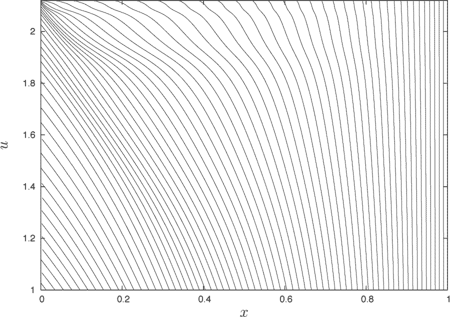
Furthermore, when half of the gridpoints have reached the origin we refine the grid and thus obtain a very simple but effective form of mesh refinement which is a crucial ingredient in the calculation of critical collapse spacetimes. In previous work [HLP+00] we have also tuned our outermost gridpoint to be located just outside of the past self-similarity horizon (SSH), the backwards lightcone of the accumulation point of the self-similar solution. Here we choose to go out all the way to null infinity. The most effective approach in this situation would be to just refine the region inside the SSH when half of the gridpoints in this region have reached the origin. While this is straightforward to implement, we found the penalty on the resolution that the original condition (the loss of half of all gridpoints) causes to be acceptable for the results presented here.
4.1.4 Accuracy and Convergence
The code is globally second order accurate. Figure 4.2 shows a convergence test for near-critical evolutions.
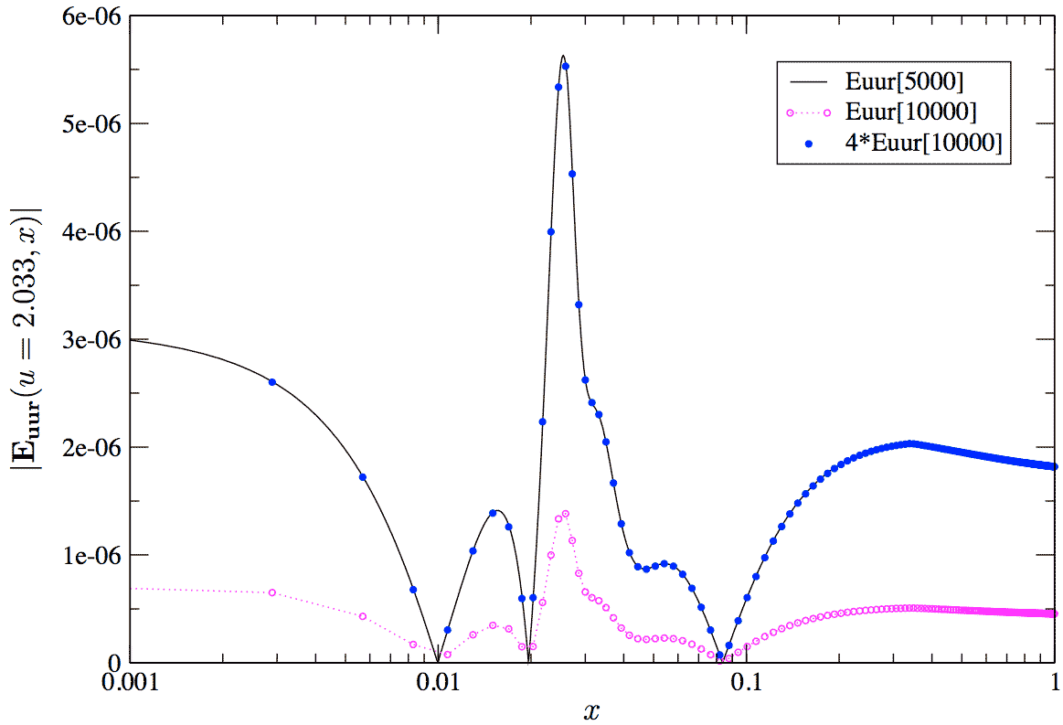
We want to emphasize that the critical value of the initial data parameter depends on the grid resolution. This fact is essential when doing convergence tests for near critical evolutions, as has been discussed in our previous paper [HLP+00].
To monitor the accuracy of the code during runs we use components of the Einstein equations which are automatically satisfied if the evolution equations hold, such as the following linear combination of the and components
| (4.1.31) |
This can be rewritten in the following form
| (4.1.32) |
where . Since this expression is a linear combination of tensor components, we use a suitably normalized quantity , where is the sum of the running maxima ( over a -slice) of the absolute values of the individual terms of . We must have for our finite difference solution to be a good approximation to the continuum solution. A convergence test for this quantity is shown in figure 4.2.
We also display numerical convergence tests (see appendix D) for and (3-level) and (2-level) in figures 4.3, 4.4, and 4.5 which show that our code computes these gridfunctions with the accuracy expected from the theoretical considerations of appendix C.3.
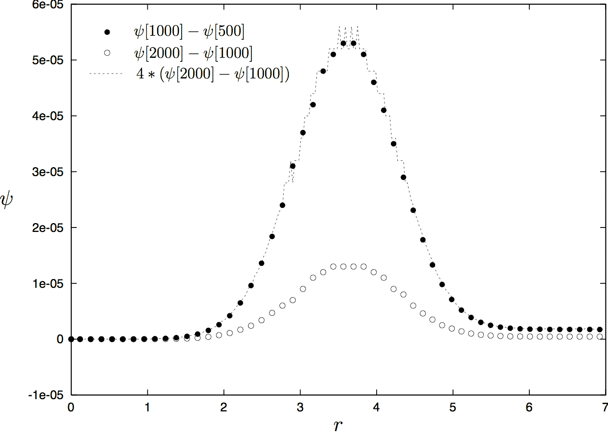
.
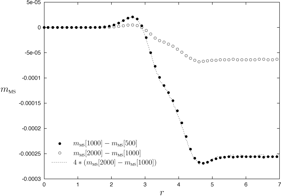
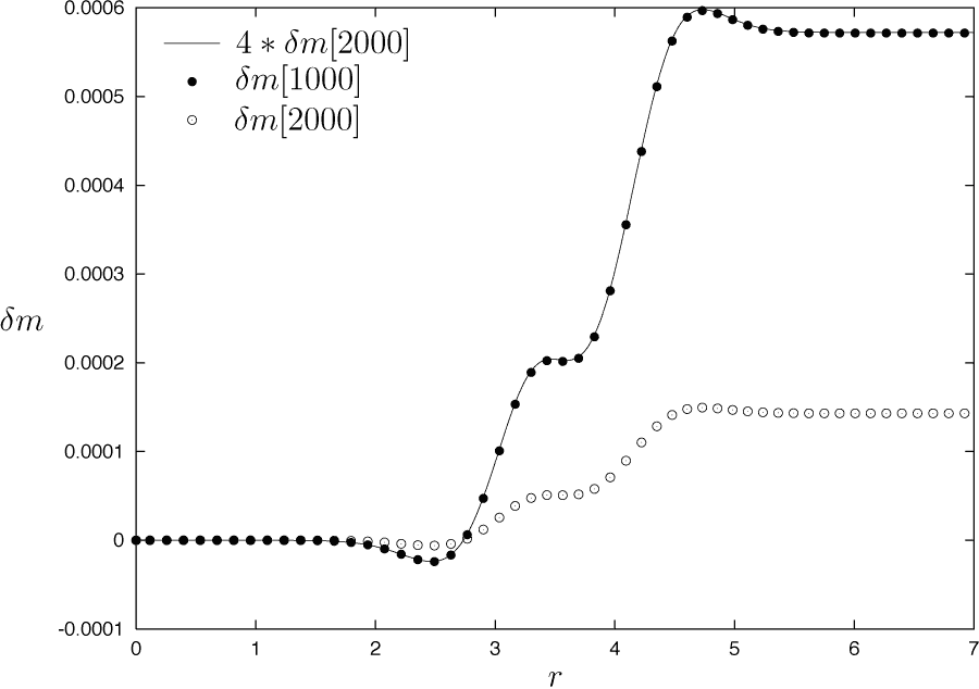
4.2 The Double-Null Code
The numerical solution scheme for the double-null code follows the work of Hamadé and Stewart [HS96] and further improvements made by Harada and Carr [Har05] which makes the scheme second order accurate.
We choose to refer to the evolution equations by the mnemonic abbreviations Dx, Ex, Cx and Sx, (with x, a number), given in section 3.8, rather than usual equation numbers.
4.2.1 Regularization
At the center of spherical symmetry we need to regularize equations E1, E2, S1 and S2 using l’Hospital’s rule. To simplify matters we use derivatives evaluated at . Derivatives of the type are straightforward to write down on an equidistant grid in and . See figure 4.6 for an illustration.
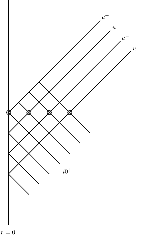
However, we need finite difference approximations for unevenly spaced grids, as our grid is only evenly spaced in and , but not in . Such finite difference approximations can be obtained by determining a low order polynomial through the required number of points and using symbolic differentiation. This is most easily done in a computer algebra system, such as Mathematica [WR05]:
For example, a second order accurate approximation of the first derivative of a function , given the function values at three points , evaluated at the point , given by
| (4.2.1) |
can be obtained by the compact expression
rgrid = {r0, r1, r2};
FullSimplify[NDSolve‘FiniteDifferenceDerivative[ \
Derivative[1], rgrid, Map[f, rgrid], \
DifferenceOrder -> 2]][[1]]
Similar expressions can be derived for higher order accuracy and second derivatives.
Depending on the number of previous slices that we have already computed, we employ different general finite difference approximations for these radial derivatives at constant . As it is not always possible to use second order accurate approximations, we have to resort to lower orders in the first two timesteps of an evolution. This is not a big problem, though, if we stick to initial data of compact support, such as Gaussian data, where the field initially almost vanishes at the origin.
To regularize the E2 equation according to l’Hospital’s rule, we take the second derivative of the numerator of the singular part of the right hand side, , using a second order accurate general finite difference stencil that requires four points. All other singular equations require only the computation of first derivatives as the denominator of the singular right hand sides are . To regularize equation S1 we compute an approximation to using formula (4.2.1), given above.
The right hand side of equation S2 is identical to that of equation S1, so that we can reuse the right hand side approximation computed for S1. As it turns out, the right hand side of equation E1 is in fact zero analytically. This is due to regularity of equation E2 which, in addition to , also forces
| (4.2.2) |
4.2.2 Initial Data
We may freely specify unconstrained data for the scalar field on an initial nullcone, usually chosen to lie at . For the sake of simplicity, we restrict considerations to Gaussian initial data:
| (4.2.3) |
Together with the specification of the gauge for the null coordinate , such as
| (4.2.4) |
we can construct initial data for all remaining evolution variables, ,,,,, and . 111Note that Hamadé and Stewart [HS96] fix the gauge by choosing It is then trivial to reconstruct and by analytic differentiation and also easy to compute :
| D2: | (4.2.5) | ||||
| D4: | (4.2.6) | ||||
| C2: | (4.2.7) |
The remaining quantities and have to be reconstructed by numerical integration:
| D5: | (4.2.8) | ||||
| E1: | (4.2.9) | ||||
| S2: | (4.2.10) |
We use Simpson’s rule (C.2.12) (and the Trapezoidal rule (C.2.11) for the first gridpoint outwards from the origin) to perform the integration.
We also apply l’Hospital’s rule for formally singular right-hand sides at the center as described in section 4.2.1. Only the equation for p is formally singular at the origin. Since we do not know any previous slices, we cannot use derivatives and instead use and the gauge choice (4.2.4):
| (4.2.11) |
Subscripts of a gridfunction denote indices on the numerical grid, starting at at the origin. Using this expression we can derive the following approximation for by applying the Trapezoidal rule
| (4.2.12) |
Similarly, we can derive an expression for by applying the Simpson rule
| (4.2.13) |
For indices we have
| (4.2.14) |
Due to the regularity of equation E2 we have
| (4.2.15) |
Using Trapezoidal and Simpson’s rules we arrive at the following expressions for on the initial slice:
| (4.2.16) |
| (4.2.17) |
| (4.2.18) |
4.2.3 Evolution Scheme
The evolution scheme evolves the massless scalar field coupled to Einstein’s equations for one time-step. In section 3.8 we have chosen to use a constrained first order system consisting of the equations E2, S1 and D2, D5, C2, D4.
Basically, since the equations to be solved are coupled ODEs, we need to alternate prediction/ correction steps in the - and -directions. We have implemented the integration of the u-equations via the explicit Trapezoidal Runge-Kutta method, equation (C.2.8), while we use the implicit Trapezoidal method, equation (C.2.7), for the v-equations to render the scheme stable. The set of discretized equations forms a nonlinear coupled algebraic system where some of the predicted function values need to be used in the correctors of other equations. The predicted value for a gridfunction is denoted by the hatted quantitiy .
First, we tackle the boundary conditions at the center of spherical symmetry . They can be categorized as follows:
-
•
algebraic boundary conditions for r, g, and f
-
•
homogeneous differential boundary conditions for a and s involving first derivatives
-
•
nonhomogeneous differential boundary conditions for p=q involving first derivatives
Depending on the number of past slices that have already been calculated, we could discretize the differential boundary conditions in a number of ways. For first derivatives at the origin we could use the following stencils:
| (4.2.19) | ||||
| (4.2.20) |
It would, however, be wrong to use those approximations, since the grid will not, in general, be equidistant in . Therefore we must resort to more general finite difference formulae as has already been discussed in section 4.2.1.
We assume that indefinite expressions (at ) of the form which occur in the right-hand sides of some of the ODE’s have already been regularized. (Again, see section 4.2.1.)
The core evolution scheme uses RK2 (explicit Trapezoidal) for the evolution equations in the -directions (the - and -equations), and implicit Trapezoidal integration for the -equations. Luckily, almost all of the resulting coupled non-linear algebraic equations in can trivially be made explicit by solving them in a fixed order. Only the - and -equations need to be decoupled by solving a linear system (See Ref. [Har05]).
Effectively, we first calculate predictor values and (via an explicit Euler step) for the -equations. Then, we proceed to calculate , , and , and finally and , which are already the final values for those quantities. Last, we correct d and q according to the RK2 explicit trapezoidal step and set the final values equal to the hatted values for and . We give a detailed description of the algorithm in pseudocode:
Evolution Algorithm:
Assuming that the boundary conditions have already been enforced at the origin gridpoint with index , we loop over all remaining gridpoints in a slice:
-
1.
Predictors
-
•
-equations: Euler forward
(4.2.21) (4.2.22) -
•
-equations: implicit Trapezoidal
(4.2.23) (4.2.24) (4.2.25) (4.2.26) (4.2.27) (4.2.28) (4.2.29) (4.2.30) If we are at the first gridpoint out from the origin (4.2.31) else (4.2.32) (4.2.33) If we are at the first gridpoint out from the origin (4.2.34) else (4.2.35) (4.2.36)
-
•
-
2.
Correctors
-
•
-equations: explicit Trapezoidal
(4.2.38) (4.2.39) -
•
-equations: trivial
(4.2.41) (4.2.42) (4.2.43) (4.2.44) (4.2.45) (4.2.46)
-
•
4.2.4 Horizon Detection and Excision
To detect apparent horizons we employ a utility function that reliably finds a possible zero in the gridfunction g[i] that represents for a given null slice . This is accomplished by looking for sign changes in the discrete gridfunction via a linear search. Such an algorithm is straightforward to implement and safe to use, as it cannot overlook zeroes. As we have discussed in section 2.4.1, due to our use of an outgoing null foliation and the causal properties of the outer trapping horizon, the function can, on a given null slice, at most have one zero, so that we can safely ignore any further zeroes as numerical artifacts.
In the code, we compute a quantity r_AH defined as the average
of r[i_left] and r[i_right], the interval bracket of the root of
g[i]. I.e. the actual zero is contained in the interval [r[i_left],r[i_right]].
We illustrate the behavior of the function by some results from numerical evolutions. Figure 4.7 shows for some null slices
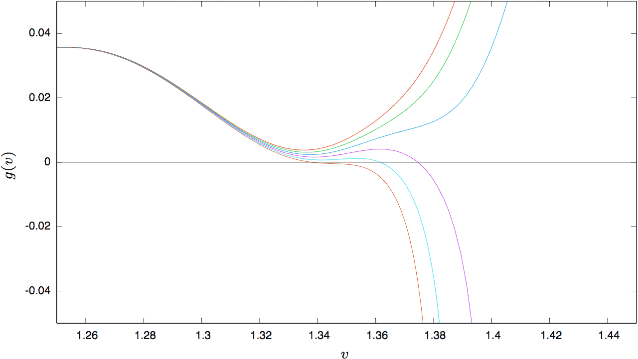
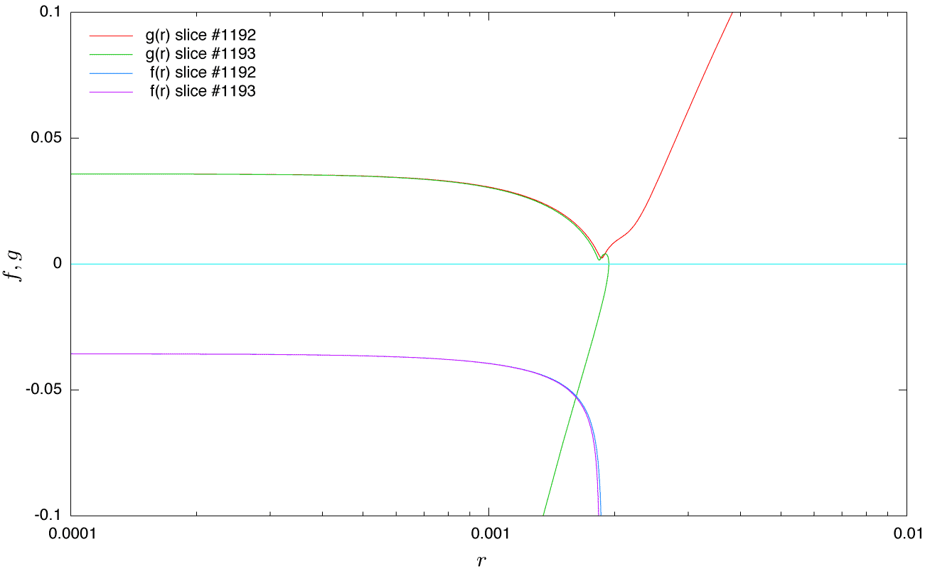

Owing to the properties of the outer trapping horizon (see section 2.2), one might assume that in a numerical collapse evolution using an outgoing null slicing the first AH is always detected at the outermost gridpoint of the slice. In practice, this is simply not the case. Due to the finiteness of the timestep, , it is highly unlikely to exactly “hit” the null slice which coincides with the event horizon. Instead, one would expect to “jump” over the event horizon and detect an AH for a and thus, since decreases with increasing (if the AH is spacelike, which it has to be if matter falls in), we detect the AH somewhere inside the grid, but not at the outer grid boundary. On a slice that penetrates the trapping horizon, all gridpoints for which are trapped and the slice bends back towards the curvature singularity at , i.e. decreases until it reaches for some . Effectively, this forces us to cut off a sizeable chunk of the grid on each slice that contains trapped surfaces: We look for trapped gridpoints, , that have fallen into the curvature singularity, that is they fulfill , and excise them and all other gridpoints that we deem too close to the singularity. This is simply done, by setting the outer grid boundary index N to a new value (smaller than the old one) such that all offending gridpoints are removed from the grid. In contrast to Cauchy evolution codes, excision is very natural and straightforward to implement in a double-null code.
4.2.5 Mesh Refinement
Although we closely follow the work of Hamadé and Stewart [HS96] in our implementation of the double-null code, we employ Garfinkle’s [Gar95] approach to increase resolution which we already described for the DICE code in section 4.1.3, rather than the more involved Berger Oliger type adaptive mesh refinement [BO84], which was also used in the seminal work by Choptuik [d’I92a, Cho93]. The application of Berger Oliger type AMR in a characteristic framework has been discussed by Pretorius and Lehner [PL04].
Concerning the mesh refinement strategy, the only difference to the DICE code, is that the double-null code is uncompactified and we can adjust the outer boundary of the grid to be slightly larger than the null ray which hits the accumulation point at of the self-similar solution as described in figure 4.10. Self-similar solutions and critical collapse phenomena are discussed in detail in chapter 5.
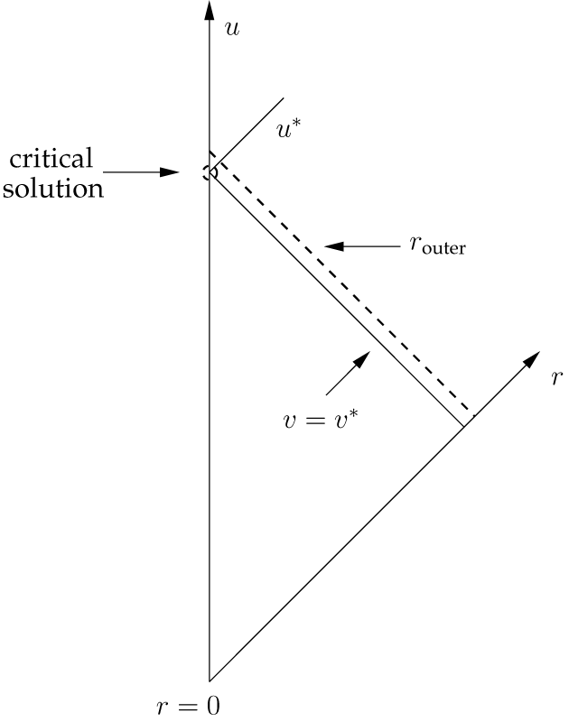
4.2.6 Constraints and Convergence
To check that our numerical solution fulfills the Einstein equations we calculate the constraint C1:
| (4.2.47) |
and suitably normalize it with the absolute value of the running maximum of its individual terms over a slice, as described in section 4.1.4. We also compute the discrete -norm of the normalized constraint. Figures 4.11 and 4.12 show the absolute value of the constraint C1 as a function of for a couple of null slices in a subcritical and a supercritical evolution, respectively.
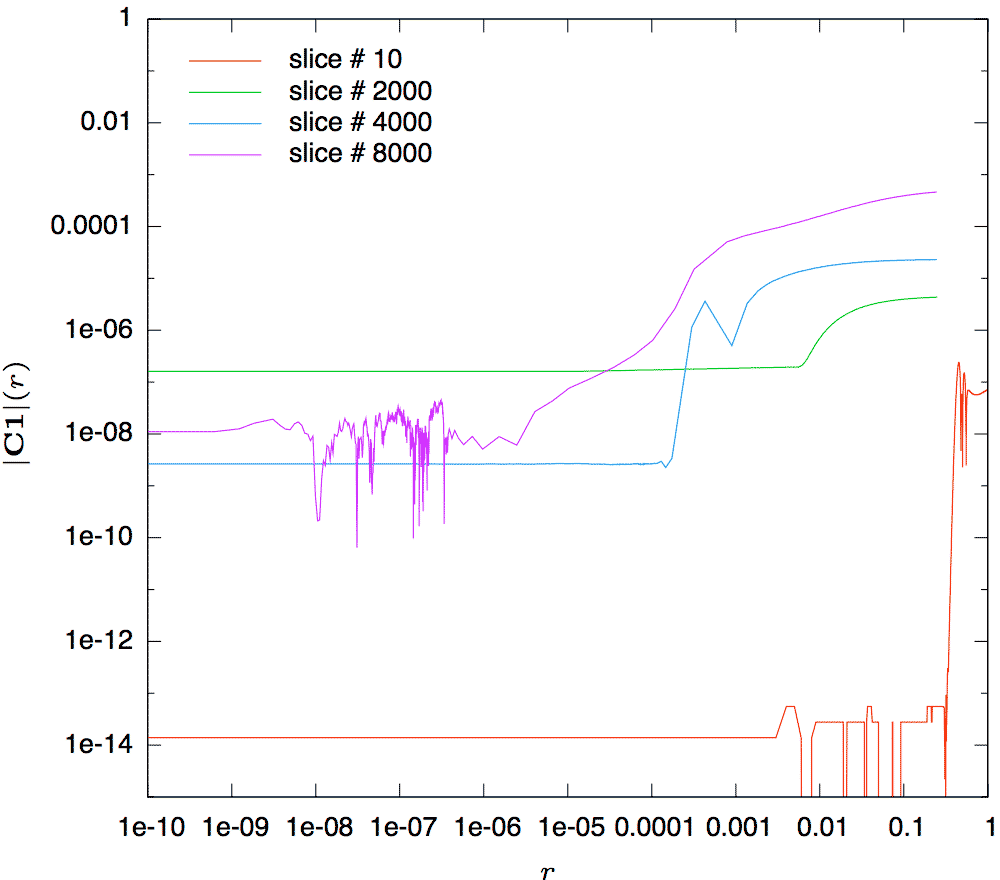
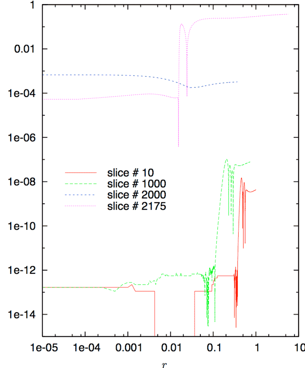
Along with the monitoring of constraint equations, convergence testing is an important strategy to ensure the correctness of numerical results, namely that, as the gridspacing tends to zero, the numerical approximation converges to the analytical evolution system according to the accuracy of the discretization. The basic methodology is explained in appendix D.
In the following, we present results from a convergence test using 1001 gridpoints as the base resolution and 2001 and 4001 gridpoints for the medium and finest resolution, respectively. As the initial data are not as close to criticality as those used in the convergence test shown in figure 4.2 for the DICE code, it was not necessary to adjust the initial data parameter for each resolution. Due to the size of the gridspacing and second order accuracy of the code, the finite difference error is approximately for the coarsest, for the medium and for the finest resolution. The set of evolutions under consideration forms an apparent horizon at approximately with a mass of . For details see table 4.1.
| N | ||
|---|---|---|
| 1001 | 1.088 | 0.00775767 |
| 2001 | 1.088 | 0.00765987 |
| 4001 | 1.088 | 0.00763467 |
As can be seen from figure 4.13 the AH is well resolved even for the coarsest resolution of 1001 gridpoints.
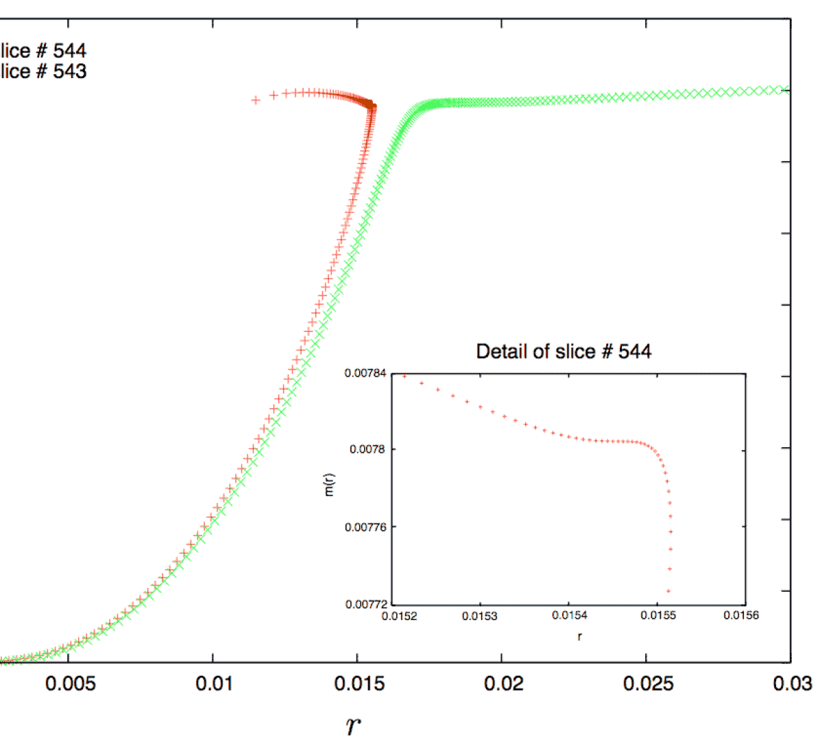
A convergence test for the -norm of the constraint C1 is shown in figure 4.14. Interestingly, the first part of the evolution exhibits fourth order convergence. Later on we have solid second order convergence. The constraint violations reach at the formation of the AH, which is the most demanding part of a collapse evolution, but otherwise are fine.
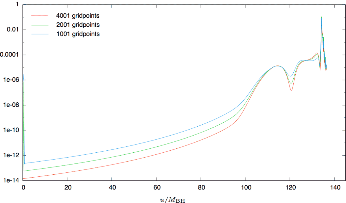
In figure 4.15 we show that the scalar field is second order convergent.
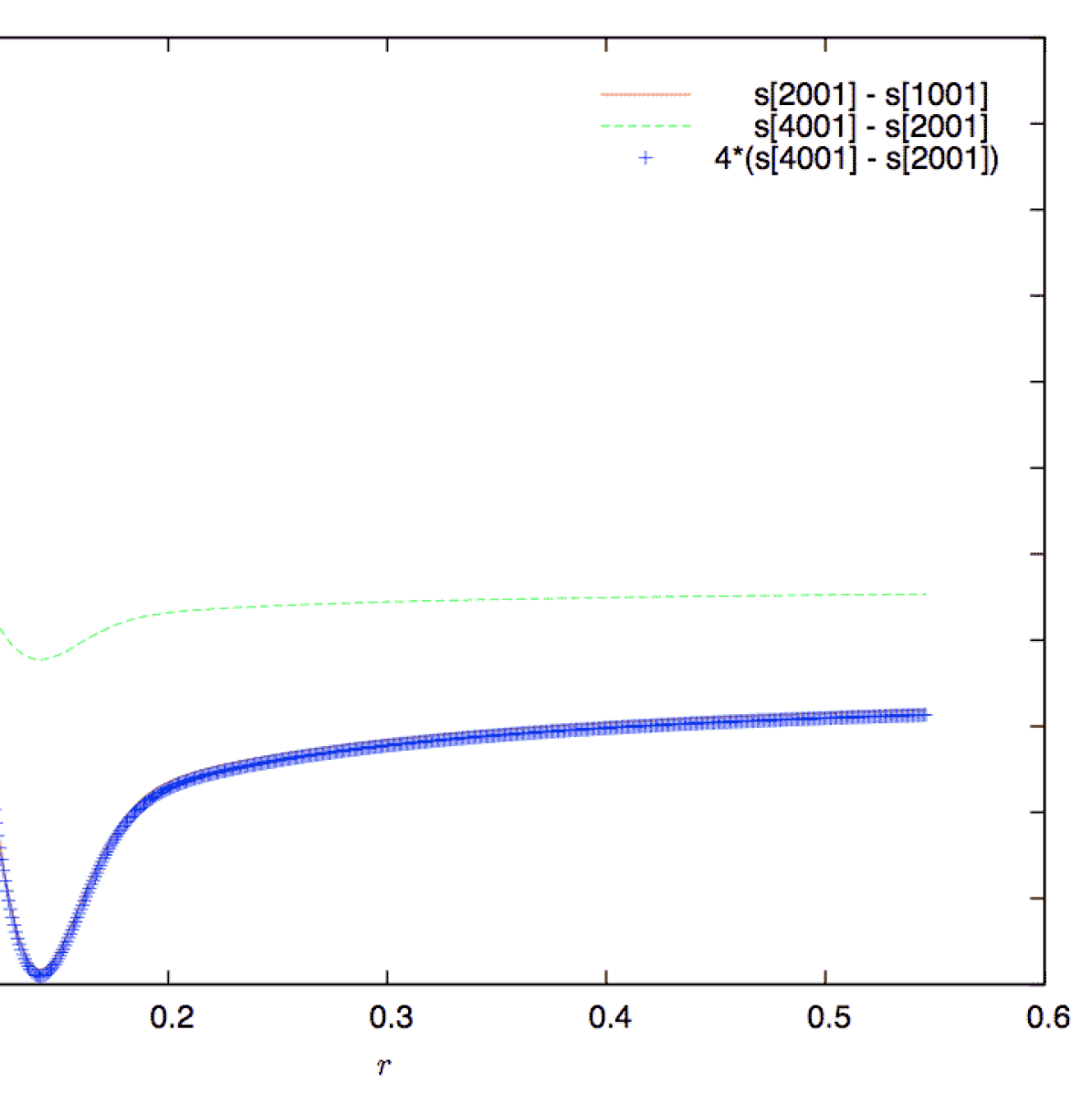
4.2.7 Timelike Observers
In the following, we describe how to calculate the proper time of an observer
from the expression (3.8.35) derived in section 3.8.3.
As the -values of our gridpoints on the double-null grid keep changing and we need to
integrate over time, we fix a set of predetermined radii r[i] and use interpolation
to obtain the corresponding set of coordinates for each slice.
We store the running integrals in a vector tp[i].
The vector is initialized at the initial slice by setting tp[i] = r[i], since we assume a flat geometry, initially.
On each null slice, and for each observer at we
-
1.
Determine and via the relations
(4.2.48) and
(4.2.49) respectively, by using cubic spline interpolation.
-
2.
Evaluate
(4.2.50) to first order accuracy.
-
3.
Evaluate using spline interpolation.
-
4.
Update the running integral by adding the term .
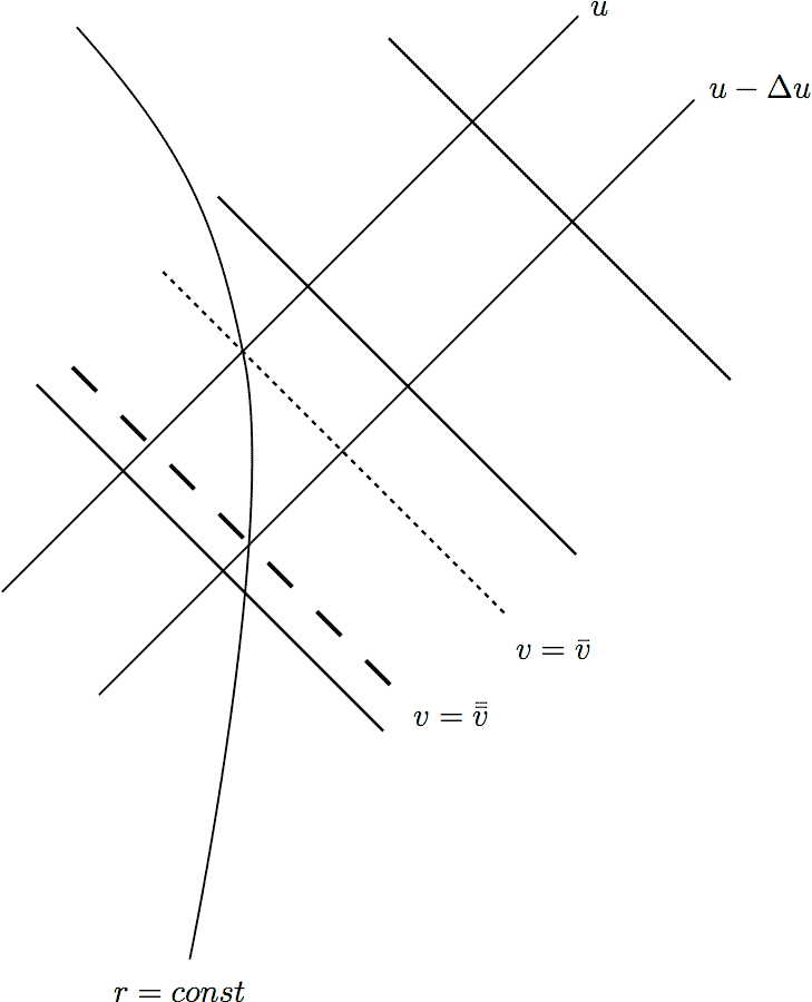
If the slice contains an apparent horizon, things are more complicated, as is no longer a single-valued function of . We first compute the index of the gridpoint with the maximum -value in the grid. We can then use spline interpolation in each of the two halves of the grid, where is either an increasing (untrapped region) or decreasing (trapped region) monotonic function of or gridpoint index. In the trapped part of a slice , so we take its absolute value in (3.8.35). We now have to keep track of one running integral for proper time for each half of the slice.
For near-critical evolutions, the trapped part of the slices is very small and hardly
warrants the difficulties incurred. Moreover, due to excision of gridpoints that come
close to the singularity at , we are missing data to compute tp[i] in the
outer half of the slice.
Chapter 5 Critical Phenomena
In general relativity, critical phenomena can be subsumed by three essential features: scaling, self-similarity and universality. They arise in the behavior of near-critical evolutions, in the course of which a universal self-similar solution is approached for some time and the idiosyncrasies of the initial data are mostly “forgotten” and replaced by symmetries inherited from the attractor. Ultimately, the self-similar solution causes the evolution to approach an endstate of the system. While self-similarity can be analyzed in single evolutions, scaling only becomes apparent when considering the final parameters of a one-parameter family of evolutions. Dimensionful quantities, such as the black hole mass, exhibit a power-law behavior with an exponent that is related to the unstable mode of the self-similar solution.
We first define the special symmetries, discrete and continuous self-similarity, that lie at the core of critical phenomena. Next, we give a qualitative description of near-critical evolutions in the dynamical systems picture. Finally, we derive the scaling law for dimensionful quantities.
5.1 Self-Similarity in General Relativity
First, we introduce the concepts of discrete (DSS) and continuous (CSS) self-similarity and then go on to talk about coordinates adapted to these symmetries. Although we are not interested in CSS per se, it is often much easier to handle and useful for modelling situations where the periodicity of DSS does not play a decisive role.
A spacetime is said to be discretely self-similar (DSS) [Gun99] if it admits a discrete diffeomorphism which leaves the metric invariant up to a constant scale factor:
| (5.1.1) |
where is a dimensionless real constant, and
| (5.1.2) |
is the pullback of the spacetime metric under the diffeomorphism and we denote the Jacobian of this map by .
Similarly, a spacetime that admits a one-parameter family of such diffeomorphisms, parametrized by , with being the identity, is called continuously self-similar (CSS). The generating vector field is homothetic, that is, it obeys the conformal Killing equation with a constant coefficient on the right hand side:
| (5.1.3) |
The choice of the constant is pure convention.
Following Gundlach [Gun97b] we introduce coordinates such that if a point has coordinates , its image has coordinates . One can then verify that DSS in these coordinates is equivalent to the condition
| (5.1.4) | ||||
| where | ||||
| (5.1.6) | ||||
To explain the connection between CSS and DSS one may introduce a vector field . The discrete diffeomorphism is then realized as Lie-dragging along by a distance . The discrete diffeomorphism cannot uniquely determine , as, loosely speaking, the vector field is free to do whatever it wants between DSS “echoing” periods.
We introduce adapted coordinates based on the Bondi coordinates defined in section 2.3.2:
| (5.1.7) | |||||
| (5.1.8) |
where is a real number which denotes the accumulation time of DSS and . A detailed derivation of these adapted coordinates is given in [Lec01]. We also require that for all such that for all . The remaining gauge freedom in is chosen such that (which is timelike at the origin) becomes null at . This null hypersurface, the backwards lightcone of the accumulation point, is known as the past self-similarity horizon (SSH). See figure 5.1 for a spacetime diagram that illustrates the behavior of these coordinates.
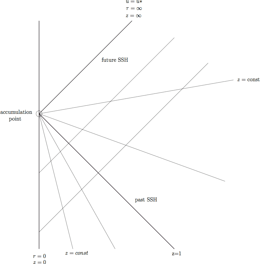
Next, we transform the Bondi line-element (2.3.17) to these new coordinates using the inverse transformation
| (5.1.9) | ||||
| (5.1.10) |
which yields
| (5.1.11) |
This line-element fulfills the condition (5.1.4) if the metric functions and are periodic in with period :
| (5.1.12) | ||||
| (5.1.13) |
Which conditions does the symmetry (5.1.1) imply for the scalar field? Clearly, matter has to share at least some of the symmetry of the geometry, as it is coupled via Einstein’s equations. First, we need to know how the Einstein tensor behaves under the action of the discrete diffeomorphism. Thanks to general covariance, the pullback of the Einstein tensor is equal to the Einstein tensor formed from the pulled-back metric:
| (5.1.14) |
It follows from the definition of DSS, equation (5.1.1), that . Because the structure of the Einstein tensor is such that in every term that contains the metric, the inverse metric also appears, and since we find and thus
| (5.1.15) |
Via Einstein’s equations this symmetry also holds for the stress energy tensor:
| (5.1.16) |
Taking the pullback of the scalar field stress energy tensor, equation (3.1.4), yields
| (5.1.17) |
where we have used the pushforward of the inverse metric,
| (5.1.18) |
and the definition of DSS in terms of the metric, equation (5.1.1). To simplify the expression we use the adapted coordinates (5.1.7) and (5.1.8), so that the point has coordinates and has coordinates and drop the angular dependence:
| (5.1.19) |
Therefore, we find the condition
| (5.1.20) |
For the scalar field, the most general ansatz compatible with DSS is (see Ref. [Gun97b])
| (5.1.21) |
The constant is determined by the component of Einstein’s equations written in terms of the adapted coordinates . As discovered numerically by Choptuik, , for unknown reasons.
The vanishing of together with the choice of the minus sign in equation (5.1.21) for gives rise to a further symmetry (see [Gun97b], [Lec01]) that has been numerically observed: If the metric functions are periodic with a period and the scalar field is “anti-periodic” with respect to this period, then, the field is obviously periodic with respect to the period . We say that the solution is DSS with period and has the additional symmetry
| (5.1.22) |
where denotes the metric functions , , and the function , while the scalar field satisfies
| (5.1.23) |
This is consistent with the fact that are even in .
5.2 General Relativity as an Infinite Dimensional Dynamical System
Following [Gun99], we give a brief qualitative introduction to the dynamical systems picture. We pretend that general relativity can be treated as an infinite-dimensional dynamical system and ignore problematic issues such as convergence to an attractor.
We restrict ourselves to isolated self-gravitating systems, such as a ball of radiation or a star. The phase space consists of the space of initial data for an isolated 111 Note that DSS or CSS do not lie in this phase space since they are not asymptotically flat. Solutions which are only self-similar inside a finite radius and asymptotically flat can be included in the phase space. system, which in our case is just the space of . Possible end-states of the system correspond to basins of attraction in phase space. The boundary between two basins of attraction is called a critical surface. We restrict attention to the existence of two distinct endstates; otherwise, more complex critical points would arise at the intersection of more than two basins of attraction. Minkowski space is an attractive fixed point in the dispersion basin, while Schwarzschild black holes form a half-line of attracting fixed points, parametrized by mass.
Consider an attracting fixed point or limit cycle, the critical solution, that lies in this critical surface, as shown in figure 5.2. We assume that this critical solution, in turn, is an attractor of codimension one in a neighborhood of phase space, which means that it possesses a single growing perturbation mode transverse to the critical surface and an infinite number of decaying modes tangential to the surface. 222 Attractors which possess more than one unstable mode would be exceedingly hard to “run into” in the course of numerical evolutions, as they would require the concurrent fine-tuning to “critical values” of more than one parameter. Trajectories starting out in the vicinity of the critical surface at first move close to the surface towards the critical solution. In the so-called intermediate asymptotics (a term coined by P. Bizon) they spend some time in the vicinity of the universal critical solution, shedding all the details of initial data from which they originated. After a while the growing mode becomes dominant and the trajectories depart towards the flat space or black hole fixed point depending on whether the data were sub- or supercritical, respectively.
In the context of this work the terms “critical solution” and “DSS solution” (or “self-similar solution”) are often used interchangeably. Due to self-similarity the DSS solution is evidently not asymptotically flat. It is however not so clear whether the term critical solution entails asymptotic flatness or not. Here, we want to make this sloppy usage more precise: We mean by critical solution an asymptotically flat spacetime which agrees in a finite region near the centre with the DSS solution, but falls off at null infinity. E.g. it would be consistent to have the exact DSS spacetime in the region defined within the backward light cone of the DSS singularity (the past self similarity horizon) and outside to fall off smoothly to infinity. Similarly, we call a solution near-critical, if it comes close to the critical solution (in the above sense) near the centre of collapse for some time during the evolution. The spacetime region in which an evolution spends in the neighbourhood of the critical solution depends on the fine tuning and the class of initial data. Therefore, the failure of the DSS solution to be asymptotically flat is perfectly consistent with its role in the dynamics of a localized object emitting radiation to null infinity.

5.3 The Black Hole Mass-Scaling Law
In this section we present an argument for the scaling of the black hole mass. We follow Gundlach ([Gun99], [Gun97b]) and Lechner [Lec01].
For the sake of simplicity, we first consider the spherically symmetric CSS case. Assume that the self-similar solution is an attractor of codimension one in phase space, that is, it has exactly one unstable mode with eigenvalue . Furthermore, assume that the system has two possible endstates, dispersion to flat space or black hole formation, such that the stable manifold of the self-similar solution divides phase space into subcritical and supercritical data. (See figure 5.2 for an illustration.) Let denote any scaling variable . We use adapted coordinates to CSS:
| (5.3.1) |
General near-critical initial data are attracted via the stable modes of the CSS solution, which we denote by . In contrast to a DSS solution, which would be periodic in the adapted coordinate , a CSS solution is independent of . In the echoing region, where dominates we write the solution as a small perturbation of the CSS solution:
| (5.3.2) |
We assume that the single unstable eigenvalue is real and positive. As all other perturbations, which are contained in , vanish. The amplitude of the unstable mode contains information on the initial data, in particular, the parameter that characterizes a one-parameter family of initial data. For so-called critical initial data, , the unstable mode is completely tuned out, so that . For near-critical data, we may then linearize around :
| (5.3.3) |
so that for suitable
| (5.3.4) |
Clearly, as , we see more and more of the critical solution. Equation (5.3.4) also sheds light on the universality of the self-similar solution: The critical phenomena are independent of the family of initial data.
Let be a value of the adapted time chosen such that the stable modes are negligible compared to the unstable mode and that the amplitude of the unstable mode equals a small number :
| (5.3.5) |
Note that depends on the initial data parameter . We rewrite this relation as
| (5.3.6) |
where the constant is independent of .
For large the linear approximation eventually breaks down when the unstable mode has grown beyond a certain bound. If, as we assume in the following, the data are supercritical, a black hole forms at late times. We emphasize that we need not follow the evolution into the nonlinear regime; it is sufficient to note that intermediate data which we can extract at depend on only through the coordinate :
| (5.3.7) |
In Bondi coordinates we have
| (5.3.8) |
The crucial point of this argument is that these intermediate data at depend on the initial data, say at time , only through the overall scale
| (5.3.9) |
The field equations do not have an intrinsic scale so that in the absence of an external scale, such as a cosmological constant, the field equations are invariant under rescalings , . Therefore, the solution based on the data at must be universal up to the overall scale.
Because the black hole mass has dimension of length in geometrized units (), it must be proportional to :
| (5.3.10) |
and we define the critical exponent
| (5.3.11) |
Relation (5.3.10) was derived independently by Koike et al. [KHA95] and Maison [Mai96].
As pointed out by Garfinkle and Duncan [GD98], it is also possible to analyze scaling in subcritical evolutions via the scaling behavior of the maximum over a whole evolution of the Ricci scalar curvature at the axis. Due to its dimension being , the Ricci scalar scales as
| (5.3.12) |
Numerically, it is easier to measure the critical exponent from the subcritical scaling of the Ricci scalar than from the supercritical scaling of the black hole mass, since one avoids numerical difficulties incurred in apparent horizon formation.
The mass-scaling relation (5.3.10) is universal in the sense that it holds for all one-parameter families of initial data, since its derivation relies on perturbations of the universal (for each model) critical solution. Thus, all solutions which approach the attractor for a while will exhibit this same scaling law.
Although the critical solution itself is not asymptotically flat due to its self-similarity, one can restrict the analysis to a region of a sufficiently large, but finite radius, so that the black hole mass is not affected.
5.3.1 DSS Fine Structure
In the case of a discretely self-similar critical solution, the scaling law (5.3.10) is modified by an oscilliatory “fine structure” overlaid on the linear relation between and . This phenomenon was first predicted by Gundlach [Gun97b] and Hod and Piran [HP97].
Similar to the CSS case, where the perturbation modes of the background solution would retain its CSS symmetry (independence of ), the modes are now periodic in and equation (5.3.2) becomes
| (5.3.13) |
Note that is not periodic in , whereas the individual modes are, since the perturbation must break the DSS symmetry or the critical solution would not be isolated [Gun97b]. Again, for suitably large so that the perturbation is still small and we can neglect the stable modes, we obtain for near-critical data
| (5.3.14) |
As before, we extract intermediate data at a time defined as
| (5.3.15) |
where is a small constant. These data depend on only through the dimensionless coordinate :
| (5.3.16) |
so that in Bondi coordinates we have
| (5.3.17) |
where . The entire solution evolved from these data scales with
| (5.3.18) |
where , (and ) are periodic functions of their argument. Therefore, the black hole mass obeys the following scaling law
| (5.3.19) |
where the constant depends on the family of initial data. Equivalently,
| (5.3.20) |
where and we have introduced the scaling exponent . As a function of , is periodic with period (for the massless scalar field). This is due to the additional symmetry of the metric functions mentioned in equation (5.1.22) (see Ref. [Gun97b]).
Chapter 6 Quasinormal Modes and Tails
6.1 Introduction
In general relativity, quasinormal modes (QNM) (see [KS99, FN98, Cha83] for a review) arise as perturbations of stellar or black hole spacetimes. Due to energy loss caused by radiation, these infinite systems do not exhibit normal mode oscillations which are characteristic of compact linear oscillating systems without damping. Instead, the frequencies become “quasi-normal”, i.e. complex, with the real part representing the frequency of the oscillation and the imaginary part representing the damping. Moreover, in contrast to normal modes, quasinormal modes do not form a complete set of basis functions.
In addition, for late times, the weak decay of the Schwarzschild potential causes the quasinormal oscillations to be swamped by the radiative tail[Pri72], which only decays polynomially in time.
In the following we give a brief review of the evolution of weak fields on a Schwarzschild background (or similar) [NF89]. The general procedure is to expand the field in spherical harmonics (according to its spin ). For each radiative multipole there is a scalar field which depends on the Schwarzschild coordinates and . Each such scalar function satisfies an equation
| (6.1.1) |
where is the effective potential and is the usual Schwarzschild “tortoise” coordinate, which is related to by .
With the ansatz we arrive at the following second order ODE that is similar to the one-dimensional Schrödinger equation for a particle encountering a potential barrier on the inifinite line[Iye87]:
| (6.1.2) |
For scalar fields the potential is
| (6.1.3) |
The effective potential behaves as a potential barrier, as it is appreciably distinct from zero only in the neighborhood of (). As the potential falls off very rapidly.
The so-called quasinormal modes of the black hole are solutions to the perturbation equation (6.1.2) which satisfy radiation boundary conditions for purely outgoing waves at (spatial) infinity and purely ingoing waves at the horizon. The real part of the QNM represents the oscillation frequency, while the imaginary part represents the decay.
The radiation produced in response to a perturbation of the field around a black hole can be divided into three stages:
-
•
radiation emitted directly by the source of perturbation
-
•
radiation due to the damped oscillations of quasinormal modes excited by the perturbation source (“ringing radiation”)
-
•
power law tails of radiation, caused by scattering of waves by the effective potential
A distant observer first records the radiation from the perturbation source, then the quasinormal ringing, which decay exponentially, and finally the radiation tails which decay much slower, by a power law, and have a very small amplitude in comparison to the first two components.
As an example, the dimensionless frequency for the mode of gravitational perturbations is , while the mode for scalar perturbations is [Iye87]. Both are fundamental modes.
To convert from the dimensionless frequency in geometrized units () to non-geometrized units, we note that the dimension of is mass/time which yields the conversion factor . The QNM frequency for a 10 solar mass black hole is then
| (6.1.4) |
and the damping time is
| (6.1.5) |
For the scalar mode, this corresponds to a frequency of and a damping time of , while for the gravitational mode, this corresponds to a frequency of and a damping time of . Compared to the Schwarzschild radius for the 10 solar mass black hole, which is , the wavelengths of the fundamental QNM are much bigger, and for the and the mode, respectively.
6.2 Quasinormal Modes In Critical Collapse
As we have mentioned, QNM excitations are, in general, obtained from linear perturbations off a fixed background, together with their associated (complex) eigenvalues. Thus, in a highly dynamical setting, such as in critical collapse evolutions, one would not expect to see (identify) quasinormal modes. However, it turns out that for our setting, the least damped spherically symmetric mode for scalar perturbations of a Schwarzschild black hole plays a relevant role.
Perturbation theory[Iye87] gives the following value for the half-period
| (6.2.1) |
where is the real part of the QNM. This mode has previously been detected in supercritical evolutions (far away from criticality) for a self-gravitating massless scalar field by Gundlach et al. [GPP94b].
In the following, we analyze radiation signals for near-critical evolutions, where the notion of a fixed background mass does no longer apply. We find that the monopole moment of the scalar field shows a damped oscillation with exponentially increasing frequency (see figure 6.1). Moreover, the sizes of the half-periods measured from one extremum to the next in roughly agree with the half-periods obtained from the least damped quasi-normal mode (QNM) of a Schwarzschild black hole with a strongly changing “background” mass as shown in figure 6.2. is obtained by evaluating at the mean value between the extrema of (which are inflection points of ).
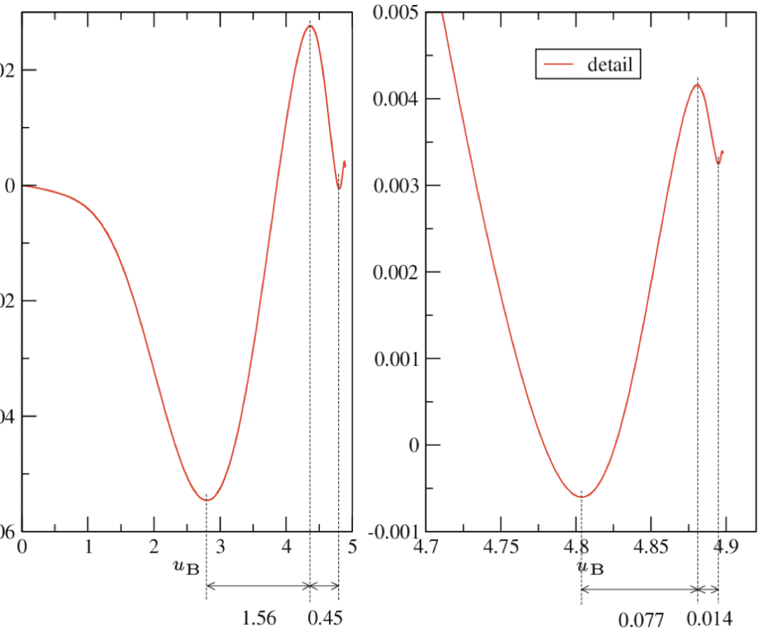
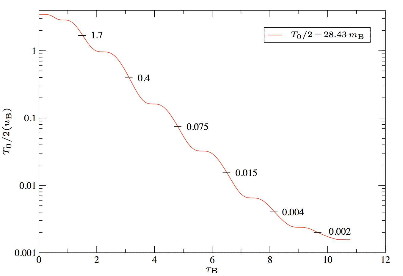
6.3 Quasinormal Modes for the Vaidya Metric
6.3.1 The Vaidya Metric
The Vaidya metric[Poi04, GS04, ACS06] is a generalization of the Schwarzschild solution with a changing mass.
We express the Schwarzschild metric in the hybrid outgoing Eddington-Finkelstein coordinates
| (6.3.1) |
where the null coordinate is defined in terms of the tortoise coordinate . Then we allow the mass parameter to become a function of retarded time: . The resulting metric is the outgoing Vaidya metric
| (6.3.2) |
The only nonvanishing component of the Einstein tensor is . For the metric (6.3.2) to be a solution of the Einstein equations the stress-energy tensor must be of the form
| (6.3.3) |
where is a radial null vector. This stress-energy tensor describes null dust, a pressureless fluid with energy density moving with a four-velocity . All the standard energy conditions [Poi04] are satisfied by if . This solution of Einstein’s equations describes a unidirectional radial flow of unpolarized radiation in the geometric optics (high frequency) approximation.
In contrast, the ingoing Vaidya metric is given by
| (6.3.4) |
and must be a monotonically increasing function of advanced time in order to satisfy the energy conditions.
Figure 6.3 shows an imploding shell of massless radiation (modelled by the ingoing Vaidya solution) which forms a black hole. For a given value of retarded time, , let the shell be contained in the interval of advanced time, i.e. let for and for . Assume that in the interval the mass-function is chosen such that no shell focussing singularity appears [Kur84]. 111According to Kuroda[Kur84], possible choices of mass-function that do not generate a shell focussing singularity are , where , or and . For observers are unaware of the infalling shell of radiation. For late times observers close to will experience tidal stresses and will begin to fall inwards. By that time, they are already trapped in the event horizon. The apparent horizon of the Vaidya spacetime is always located at [Poi04].
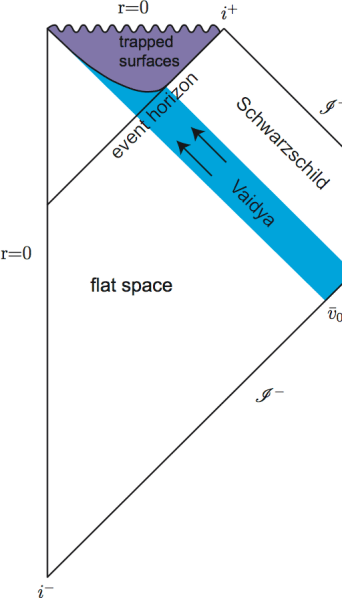
6.3.2 QNM Modes in a Vaidya Background
The analysis of QNM for time-dependent situations, such as accretion processes or Hawking radiation is discussed for the Vaidya metric by Abdalla, Chirenti, and Saa in [ACS06]. Building on earlier work by Girotto and Saa[GS04], they employ a semi-analytical approach in which one considers the Vaidya metric in double-null coordinates ab initio. After choosing a smooth mass-function , it is possible to numerically reconstruct the metric functions. Then, scalar (or electromagnetic) perturbations on the constructed Vaidya background are evolved using a characteristic algorithm. Analysis of the perturbation field close to the event horizon then yields estimates for the real and imaginary parts of the QNM.
The authors point out the existence of a stationary adiabatic regime where the real part of the QNM varies inversely with the mass-function, just as one would obtain when modelling the Vaidya solution as a series of Schwarzschild slices with changing mass as we have done in section 6.2. In addition, they formulate a heuristic criterion that indicates when to expect the appearance of non-stationary behavior:
| (6.3.5) |
The non-stationary behavior manifests itself as an inertial effect in the real part of the QNM: no longer behaves as , as one would expect for a stationary adiabatic regime.
In the following, we apply their criterion for non-stationary behavior to our numerical results. Note that we measure the QNM at and we are dealing with a monotonically decreasing function, the Bondi mass . 222The DICE code from which these results have been calculated cannot penetrate apparent horizons, and, at least for critical collapse, we have not been able to read off QNM close to the event horizon. In section 6.2 we have observed that the real parts of the fundamental scalar field QNM roughly agrees with its Schwarzschild value (for a decreasing mass) during critical collapse. We have verified this (see figures 6.1, 6.2) by comparing the half-periods measured from one extremum to the next in with the half-periods predicted by perturbation theory with a strongly changing background mass .
We have also tried to read off the imaginary parts of the QNM from , but to no avail: One the one hand, this is very difficult, because we do not have many oscillations to accurately measure the decay. But, more importantly, as shown in figure 6.4, behaves as . This is due to self-similarity, since the monopole moment has dimension of length. We note that we have corrected a slight offset in .
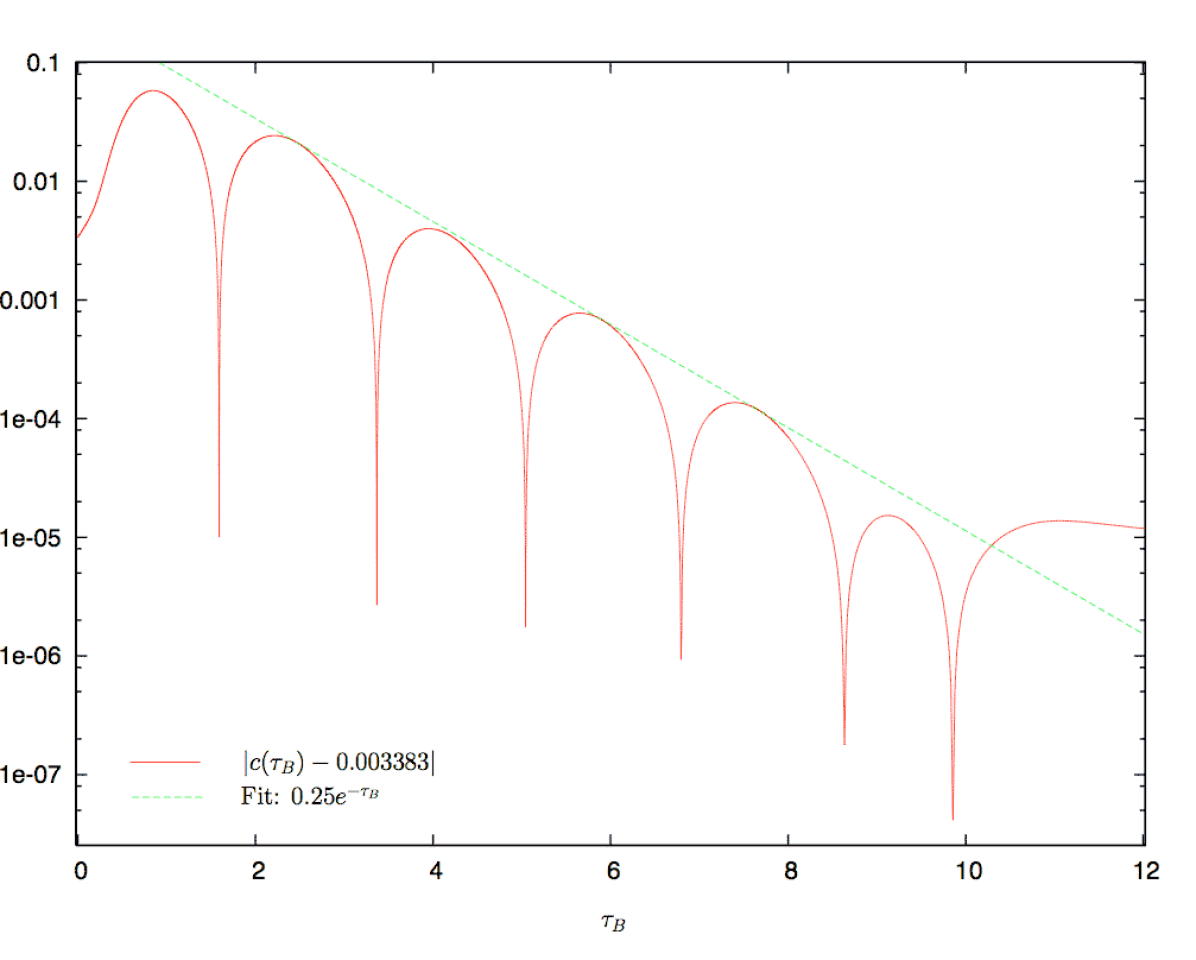
Instead of directly reading off the imaginary part of the QNM, we can still estimate the decay from perturbation theory for a few background masses and compare the result to in order to check that the non-stationarity criterion mentioned above, (6.3.5) is not fulfilled. As can be seen in the figures 6.5 and 6.6, stationarity is well satisfied with the exception of the very late stages of collapse, where we leave the self-similar regime and approach black hole formation.
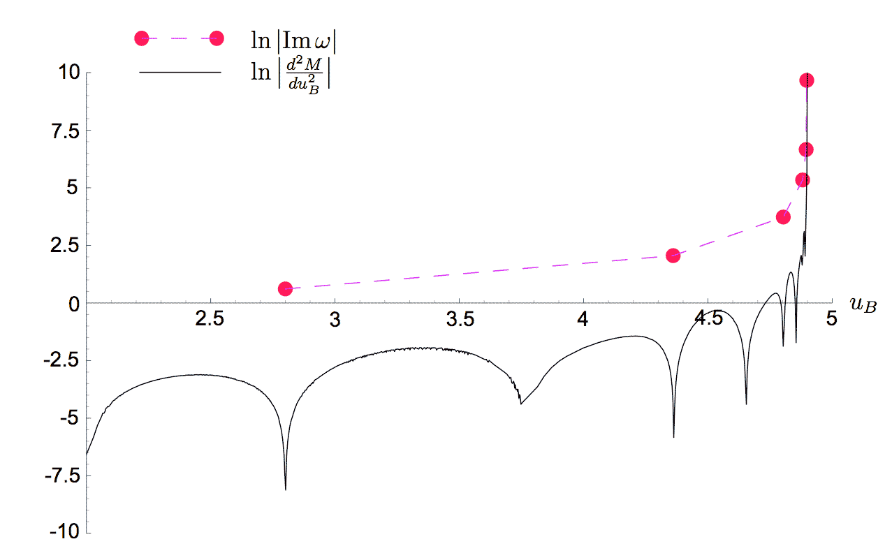
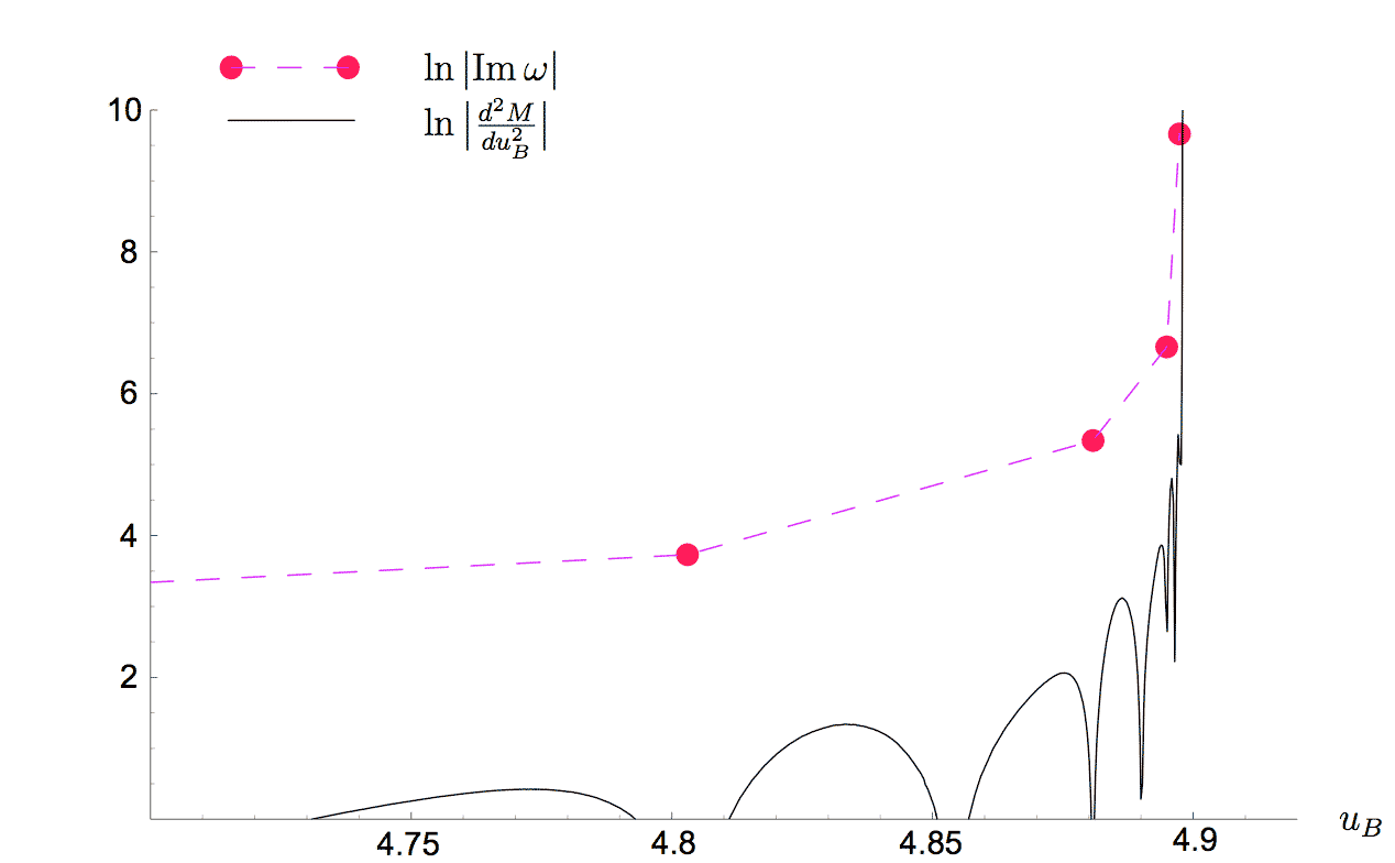
.
6.4 Power-law Tails
As has been established by Price [Pri72], perturbation fields outside of Schwarzschild black holes die off with an inverse power-law tail at late times. In contrast to quasinormal modes this behavior does not depend on the details of the collapse process, but only on the asymptotic falloff of the effective potential; (i.e. in a curved spacetime, wave propagation is not confined to the light cones, rather waves spread inside the light cones, due to scattering off spacetime curvature.) Therefore, tail phenomena can be observed independently of the endstate of the evolution. For Gaussian initial data the Newman-Penrose constant [GWS94] vanishes and for late times perturbation theory [GPP94a, GPP94b] predicts that the field falls off as near and near timelike infinity .
To be more precise [Bar99a, Bar99b], consider a distant static observer at and Bondi time elapsed since the “main pulse” of radiation has reached the observer (the duration of the main pulse has been assumed negligible in [Bar99a, Bar99b]). Null infinity is then found to be approximated by the region where within the context of a perturbative analysis of tail behavior [Lea86a, Lea86b, Bar99a]. This regime has been termed the “astrophysical zone” by Leaver [Lea86a, Lea86b, Bar99a].
In addition, the convergence of the perturbation expansion in [Bar99a, Bar99b] requires , where is the mass of the background. In our case, the mass which gives rise to the effective potential is bounded from above by the mass of the initial (ingoing) pulse, . Therefore, we demand that . Numerically, we observe tails only for .
Closeness to timelike infinity, on the other hand, demands , where is the usual “tortoise” coordinate . In figure 6.7 we show power-law exponents determined by fits of at different curves over a series of time intervals for a subcritical evolution. As described in section 4.1 we use spline interpolation to calculate . The exponents have been determined by fitting the field at against a power of in 5 distinct time intervals of the evolution. The domains of validity of the exponents predicted by perturbation theory, near and near , can be observed here. It is clear that the outermost gridpoints in this evolution (using 10000 gridpoints) are indeed located in the “astrophysical zone” since , where is the Bondi time elapsed since the main pulse of radiation has reached the observer at about (see figure 6.8). On the other hand, closeness to timelike infinity demands that . Note that for , where is the initial Bondi mass. It is also apparent that for the observers are in between the two zones and the power-law exponents seem to change smoothly.
Figure 6.8 displays the power-law decay, with exponent , of the Bondi mass for the same subcritical evolution. This behavior can be explained by integrating the Bondi mass-loss equation (3.7.13) with in the regime of power-law tails.
Note that in situations involving realistic sources and realistic detectors, power-law tails only play a minor (if any) role as an actual signal, but the power-law tail results still can provide hints on how to resolve the very important question of whether null infinity is a useful idealisation for gravitational wave detectors. Accordingly, we suggest to generalize the term “astrophysical zone” to more general, non-perturbative situations, by re-enterpreting – in a very loose sense – as a suitably chosen large time scale characteristic of the source. The physical idea is that the distance from observers of astrophysical phenomena, e.g. gravitational wave detectors, to the radiation sources is very large compared to the time during which substantial radiation from the source can be observed. This is at least expected for sources where general relativity is important, as opposed to problems for which a (Post-) Newtonian approach and the quadrupole formula are sufficient. An example would be a binary black hole merger in another galaxy, which might have a characteristic dynamical time scale of a fraction of a second, and which might be observed during several thousand cycles, including a portion of the QNM ringdown.

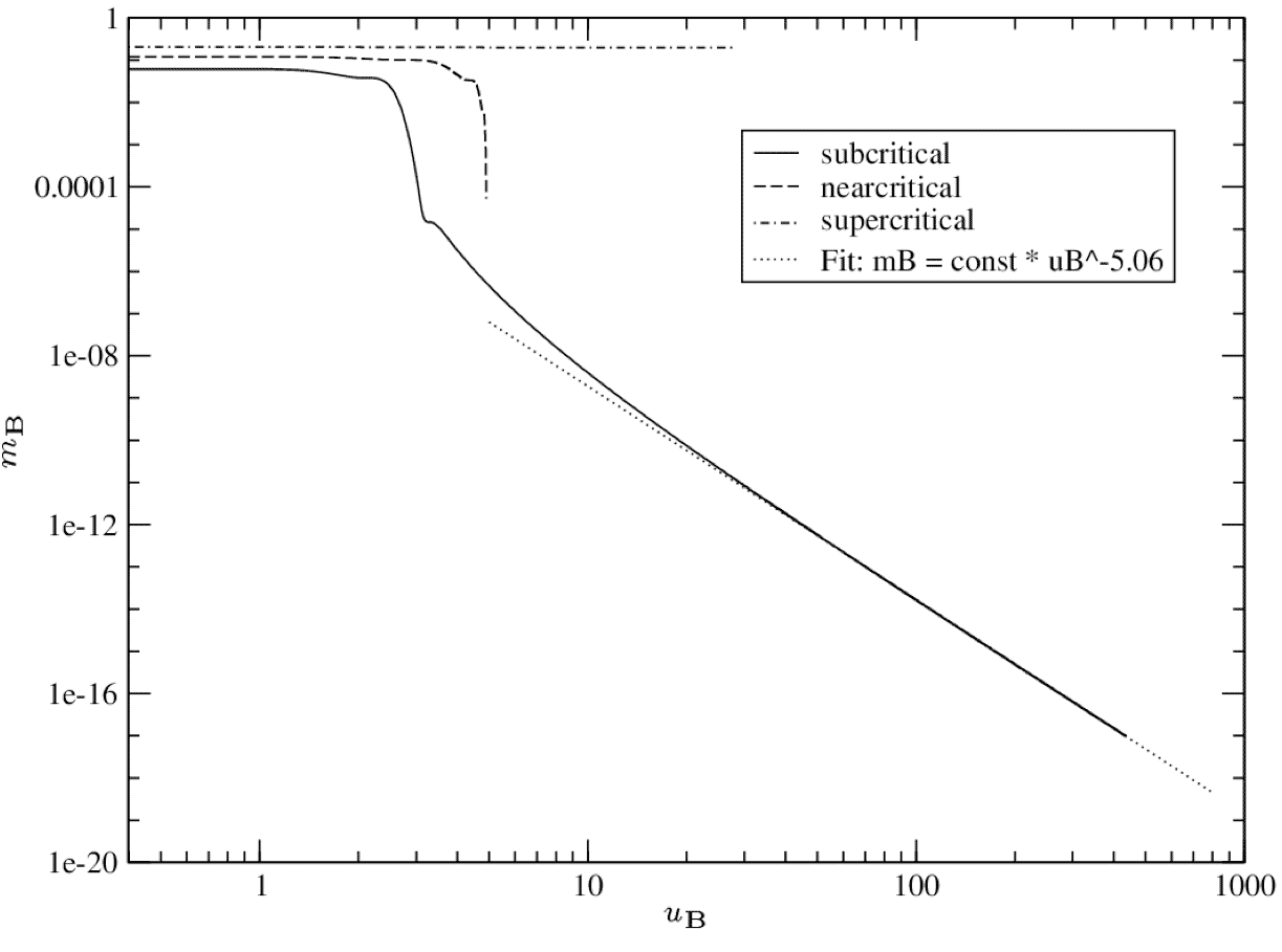
Chapter 7 Numerical Evidence for Critical Phenomena
In this chapter we present numerical results of critical behavior in the Einstein-massless scalar field system computed using the DICE code and the double-null code.
Section 7.1 focusses on results from the compactified dice evolution code which stress the global observability of critical phenomena at future null infinity. We also show results from uncompactified evolutions for cases in which we did not have compactified results available. We would like to emphasize that for the local detection of discrete self-similarity, inside the past self-similarity horizon, as discussed in section 7.1.3, both DICE codes are basically equivalent, the uncompactified DICE code having a slight edge over the compactified code as to resolution.
The results of the double-null code shown in section 7.2 complement the local picture given by the DICE code. The double-null code is uncompactified but, in contrast to the DICE code, it can penetrate apparent horizons and thus enables us to probe supercritical spacetimes a little longer. The reason for introducing this code was mostly to analyze the fate of the exterior mass that accumulates outside of the past self-similarity horizon in near-critical evolutions, as will be discussed in section 7.1.2. Moreover, it is always preferable to have more than one way of computing a numerical result, which, by comparison, allows us to rule out numerical artifacts specific to a particular numerical scheme.
7.1 Results from the DICE Code
7.1.1 Identification of Critical Behavior
We consider one-parameter families of initial data , such that for small values of we have dispersion, while for large values of we have black hole formation. It has been found numerically [d’I92a, Cho93] that, for any initial data family considered, the evolution of near-critical data approach a universal DSS critical solution. In this thesis, we assume universality and restrict ourselves to Gaussian-like initial data
| (7.1.1) |
where . This choice makes it easy to compare compactified to uncompactified evolutions using the same initial data. All results from the compactified DICE code presented here use and and a radial resolution of gridpoints, unless stated otherwise. The criticality parameter is identified with the amplitude .
As has become common practice, we find near-critical data through a bisection search in . This procedure yields in particular a numerical approximation to the critical value which defines the threshold of singularity formation.
In the bisection search, a number of criteria are possible to distinguish dispersion from collapse. Their equivalence can be checked a posteriori when comparing the final result, i.e. subcritical and supercritical solutions close to criticality. A typical criterion is to monitor the ratio , where signifies the presence of an apparent horizon. This criterion has been used successfully also in combination with slicing conditions, that do not penetrate apparent horizons – as is the case in our approach. Remarkably, in practice it turns out, that is a sufficient criterion to mark a scalar field evolution as supercritical. For practical and historical reasons, this is the approach we have adopted for our code.
A number of other options come to mind, in particular in our context of evolving out to null infinity, one could e.g. monitor the redshift (2.3.46) or Bondi mass. In a dispersion evolution, the redshift will decay to zero, while it will approach infinity when a black hole forms. Similarly, the Bondi mass will decay to zero with a characteristic tail behavior, as is shown in Fig. 6.8, in a dispersion evolution, and will asymptote to a (positive) constant when the field does not disperse.
The local detection of discrete self-similarity and extraction of the critical echoing parameter from a near-critical numerical evolution is discussed in section 7.1.3. Here we are concerned with the global picture: In the course of a near-critical evolution, remnants of the self-similar dynamics which occur locally, inside the SSH, are radiated to future null infinity. Remarkably, we observe that the imprints of DSS behavior are still present in asymptotic quantities such as the news function and the Bondi mass (see figures 7.1 and 7.8).
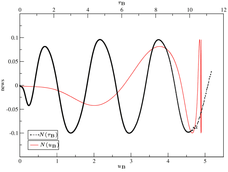
To further test the accuracy of the compactified DICE code in the asymptotic regime, we have plotted the left and right hand sides of the Bondi mass-loss equation, (3.7.12), in figure 7.2. Figure 7.3 shows the redshift factor, equation (2.3.46), for the same evolution.
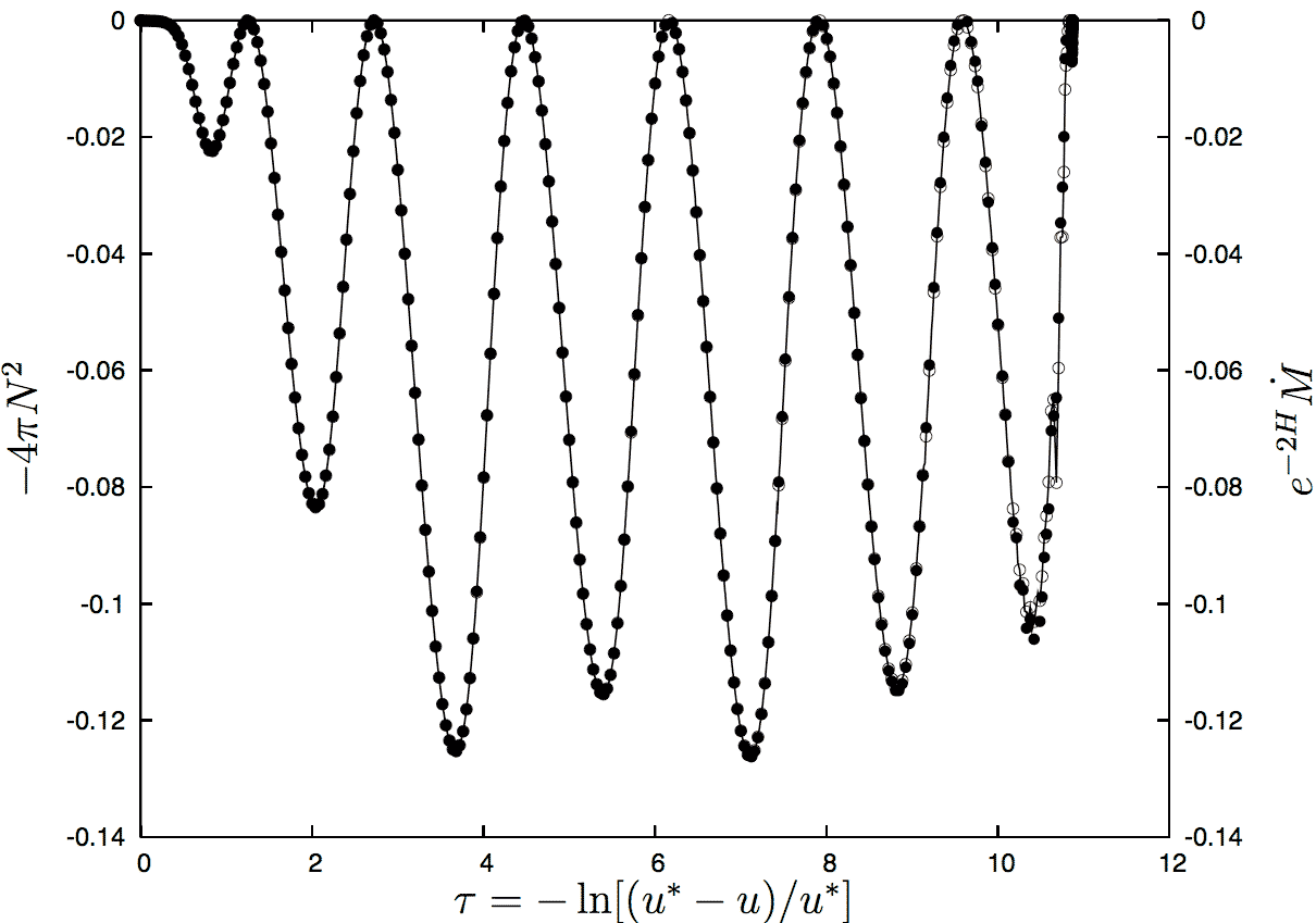
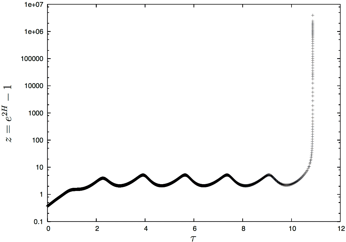
In addition, in numerical evolutions of supercritical data, the black hole mass has been found to exhibit a universal scaling law (5.3.20), in accordance with the discussion in section 5.3, (see [HP97, KHA95, Gun97b]):
| (7.1.2) |
where and the function is periodic with period in . Figure 7.5 shows this scaling behavior of the mass. To analyze the fine-structure of the mass-scaling law, one conveniently runs a series of evolutions with masses spaced linearly in . One also needs to ensure to measure the mass of the outermost component of the horizon in order to obtain the fine-structure of the scaling law shown in figure 7.4.
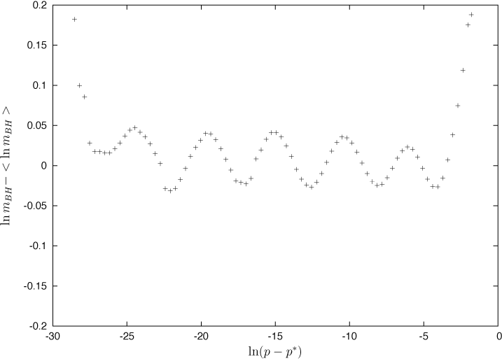
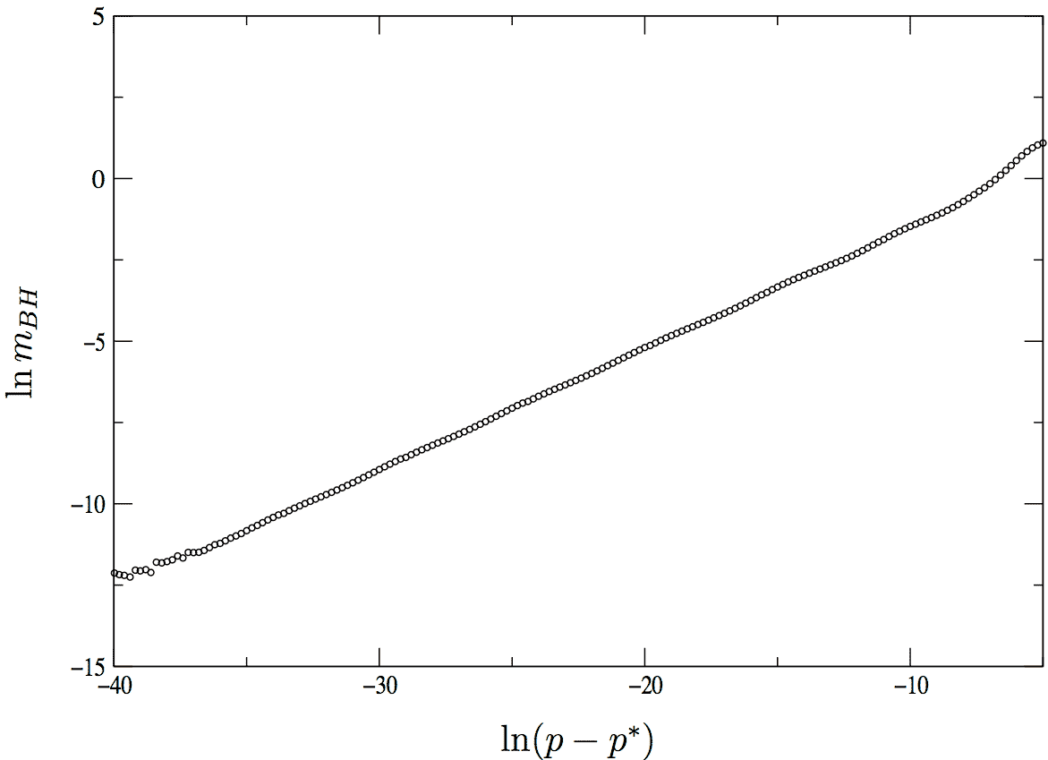
This scaling law has been derived by arguments based on linear perturbation theory around the critical solution and dimensional analysis however without using a precise definition of the black hole mass [HP97, Gun97b]. A typical approach in numerical simulations based on coordinates that do not penetrate apparent horizons, as far as we are aware, is to follow a peak in until this quantity almost reaches unity, at which point the simulation is usually slowed down by a CFL-type condition, and then read off the approximate horizon mass at this point. We follow this heuristic approach, and are able to reproduce the mass scaling and fine structure.
At least conceptually, this approach is problematic without quantifying how much mass-energy still remains outside of the peak in where the horizon-mass is read off. From the perturbation theory argument, one expects scaling behavior only for quantities within the self-similar region of spacetime, which does not necessarily extend beyond the SSH. We will return to this point in the discussion section 8.
We have found that the mass scaling law for compactified evolutions exhibits a ”leveling-off” effect for strongly fine-tuned evolutions. Figure 7.6 shows that for the logarithm of the detected black hole mass is constant, while further away from criticality, the scaling agrees with the expected power law behavior given in equation (5.3.20). The fact that this constant is resolution dependent, i.e. it decreases with increasing resolution, indicates that it is a numerical artifact of the compactified code.
In contrast, uncompactified evolutions generated by the DICE code where the outer grid boundary has been adjusted to be close to the ingoing null ray, , that hits the accumulation point, are completely unaffected by this leveling off in the scaling law (see figure 7.5). Nor are codes affected that penetrate the apparent horizon and base their horizon detection on the first actual apparent horizon detected on a slice, such as our double null code (see figure 7.18 in section 7.2.1).
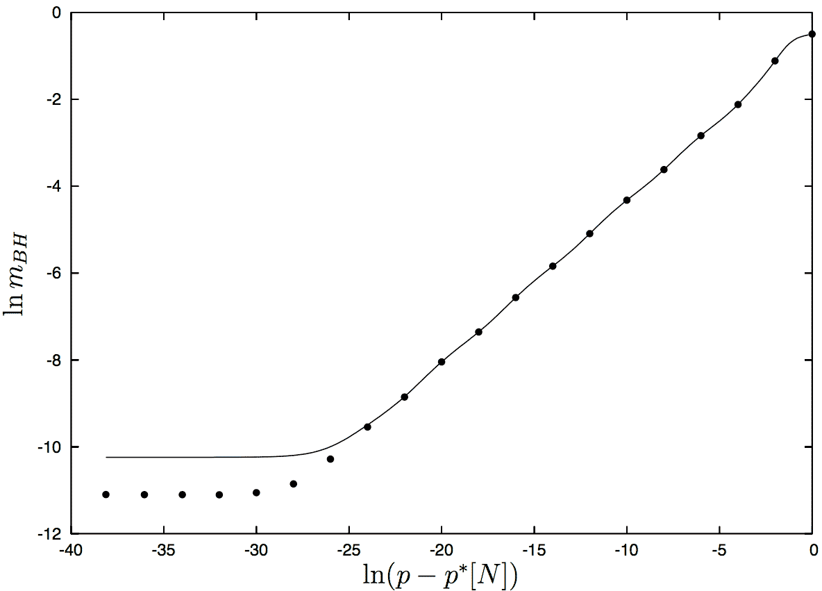
Note that for a near-critical solution, the approximate value of the accumulation time naturally defines an approximate location (i.e. advanced time) of the SSH.
For observers at null infinity, a natural time coordinate is Bondi time as defined in eq. (2.3.35) – Bondi time can be identified with the proper time of timelike observers at large distances – see the discussion in Sec. 8. In order to analyze critical phenomena, we define a time coordinate which is suitably adapted to self-similar critical collapse and set
| (7.1.3) |
The adapted time coordinate can be defined for spacetimes which are close to the critical solution inside of the SSH, so that the value of the accumulation time can be determined by a fit to periodicity in . We have used a fit to periodicity of the news function – is periodic with period after the spacetime has come close to the critical solution (see figure 7.1).
Note that is only an approximate adapted coordinate since it depends on the relation between Bondi and central time (2.3.35). In order to gain some insight into the behavior of consider the simpler case of a CSS collapse. We assume that changes only little outside the past SSH, i.e. . Then, since in the CSS regime, we find by integrating (2.3.35) that
| (7.1.4) |
where and we have chosen the initial condition . Furthermore, it follows from the definition of the adapted time coordinates, equations (5.1.7) and (7.1.3), that
| (7.1.5) |
in the CSS regime. Numerically, the deviations from this relation for the DSS case turn out to be quite small. We cannot expect this relation to hold, if the mass outside the past SSH is large compared to the inside, which we observe in the very late stages of strongly fine-tuned evolutions. Nevertheless, we have still been able to resolve DSS phenomena using the coordinate (see fig. 7.8).
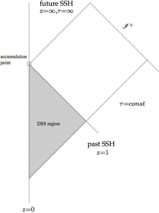
7.1.2 DSS Behavior in the Bondi Mass and the News Function
The following argument suggests that the news function is approximately periodic in , as shown in figure 7.1. Assume effective DSS data for the scalar field and the metric functions on the past self-similarity horizon (SSH) (see figure 7.7). Moreover, we assume that the contribution of the right hand side integral in the wave equation for the scalar field (3.5.1) can be neglected outside of the SSH, such that the DSS data on the SSH are linearly propagated to without backscattering, i.e.
| (7.1.6) |
Furthermore, assume that changes in outside of the SSH are small, so that . It then follows that
| (7.1.7) |
which shows that the news function is approximately periodic in (and in if equation (7.1.5) holds) with period and satisfies .
In order to determine the behavior of the Bondi mass, we can then rewrite the Bondi mass-loss equation (3.7.13)
| (7.1.8) |
Since is -periodic in , then takes the following form
| (7.1.9) |
where is -periodic in .
This behavior mimics the behavior of the mass-function: We rewrite the mass-function in adapted coordinates , using (5.1.8),
| (7.1.10) |
and evaluate it at the SSH, which, by a judicious choice of the periodic function can be chosen to be at (since the past SSH is a null surface, one needs to ensure that becomes null at ). We obtain
| (7.1.11) |
where is periodic with period .
The periodicity and exponential decay of and are confirmed by our numerical calculations (see fig. 7.8). Note that the Bondi mass levels off at roughly of the mass in the initial configuration, whereas the mass contained within the backwards light cone continues to scale according to the prediction of critical collapse evolution, equation (7.1.9). Since the difference, i.e. , is almost zero at the initial slice, we conjecture that, at late times, is the energy due to backscattering in a critical evolution. We do not have a physical explanation for the oscillations seen in for earlier times. This behavior may, however, be due to errors in the determination of the location of the past SSH. In figure 7.9 it is apparent that is localized in a region outside the past SSH.
We observe that contained in a slice close to horizon formation is almost constant for different near critical evolutions (down to the numerical limit of fine tuning). In the very late stages of the evolution, the growing redshift, effectively halts the numerical evolution, while the error norm approaches .
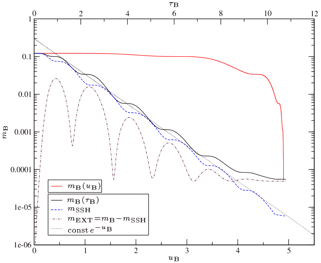
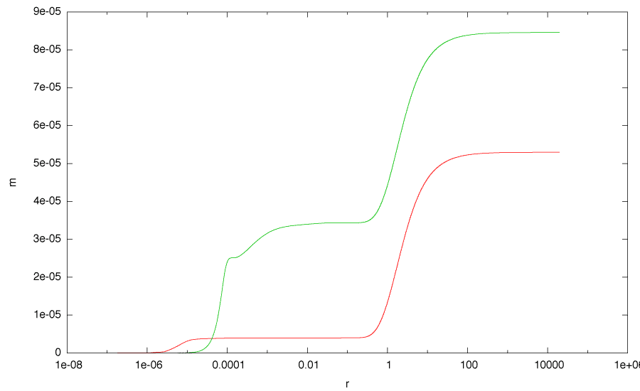
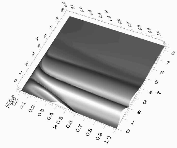
7.1.3 Local Detection of Discrete Self-Similarity
We discuss some methods to extract the echoing exponent of discrete self-similarity from a near-critical numerical evolution while restricting attention to the past self-similarity horizon.
max(2m/r)-Plots
The black-hole formation diagnostic furnishes a necessary condition for discrete self-similarity, namely periodicity in the function
| (7.1.12) |
where the maximum is taken over null slices and denotes the mass-function in spherical symmetry, as defined in equation (3.7.1).
The viability of this approach depends on the choice of initial data. For the usual Gaussian initial data family, experience shows that the maximum is well-defined. For other choices, such as the double-Gaussian initial data of section 7.2.4, two (or more) peaks in may compete with each other and thus the maximum can jump from one slice to another.
The echoing exponent can be determined by analyzing plots of vs. and adjusting such that successive echoes obey a constant spacing, which equals . In practice, a crude estimate of can be obtained in slightly supercritical evolutions as the coordinate time of the formation of the (small) black hole. This process can be carried out by hand or automatized by a fitting procedure. The initial transient in which the system first approaches the vicinity of the attractor has to be ignored. The result of such a fit is shown in figure 7.11.
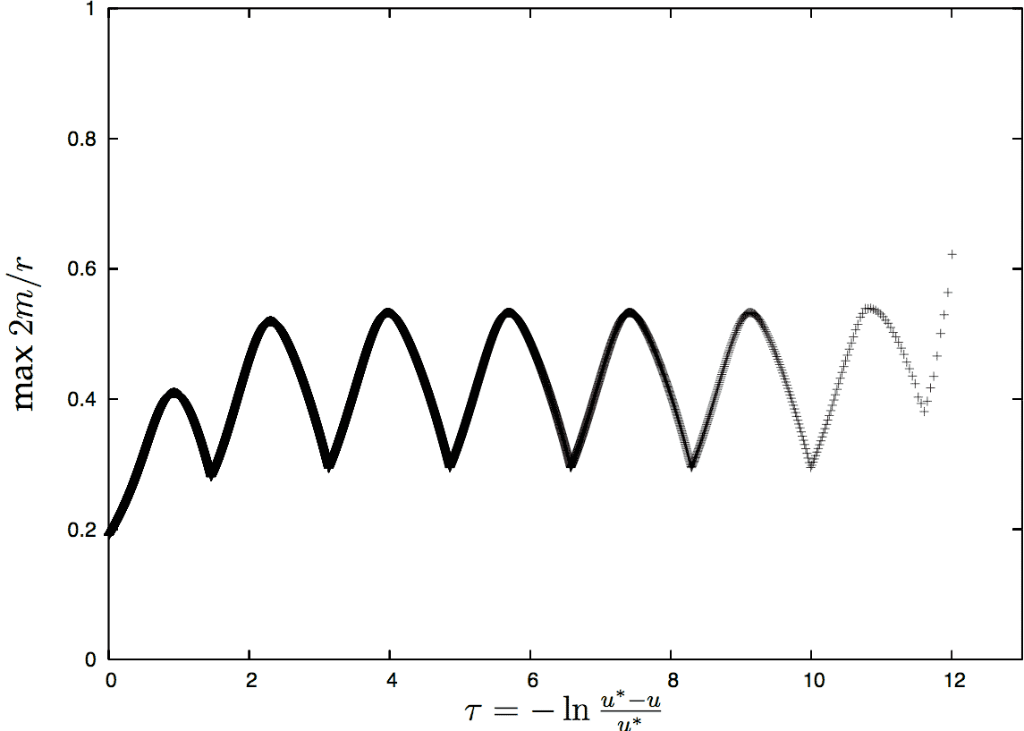
DSS-Snapshots
Although plots of the diagnostic are handy for determining and , since they are easy to generate, they do not encompass the full scope of DSS, since, by taking the maximum, the information available is collapsed down to just one data point per null-slice. Given a function on spacetime which is DSS, it shows this behavior at any given radial position. This much stronger criterion can be investigated with the following method (adapted from [Cho98]).
In coordinates DSS corresponds to a logarithmic rescaling in both time and space. As has been discussed in section 5.1, in adapted coordinates DSS amounts to
| (7.1.13) |
Here, we prefer to use instead of . From the definition of ,
| (7.1.14) |
observe that
| (7.1.15) |
Thus, the following equality holds
| (7.1.16) |
and, for a given , and using , we have
| (7.1.17) |
Successive frames in the plots shown in figures 7.12 and 7.13 are equally spaced in the adapted time coordinate . The quantities are plotted against with appropriate “shifts” in the null slices according to equation (7.1.17).
While dimensionless quantities (, , , ) are mapped according to (7.1.17) without a change of scale under the diffeomorphism associated with DSS, dimensionful quantities such as or also scale according to their dimensions, e.g. and thus
| (7.1.18) |
As an example, figure 7.14 shows the scalar field and its image under the DSS diffeomorphism.
To be able to more clearly visualize discrete self-similarity, we show the scalar field as a function of and for a near-critical compactified evolution in figures 7.15 and 7.16. Figure 7.17 depicts the ingoing null geodesic that hits the accumulation point of the DSS-solution.
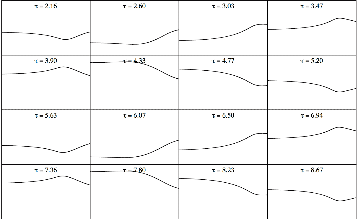
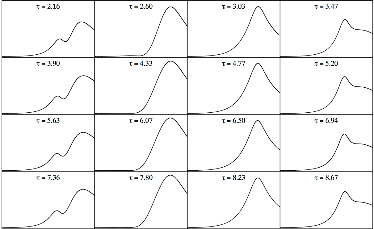
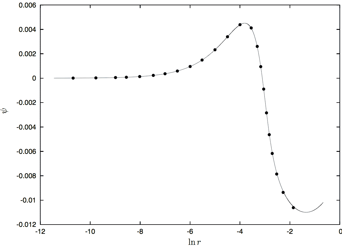
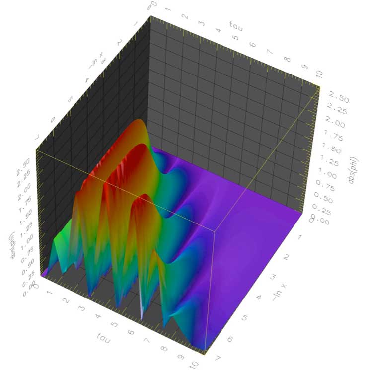
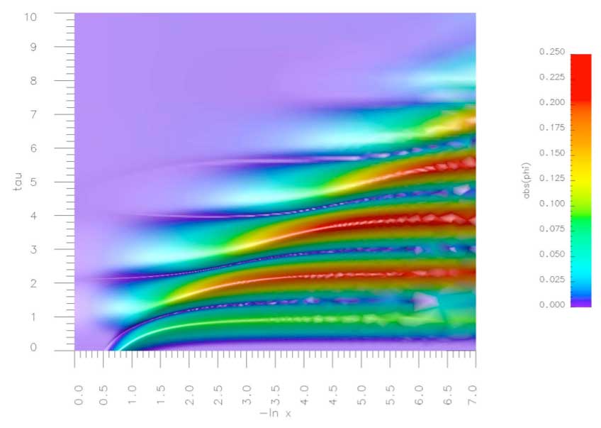
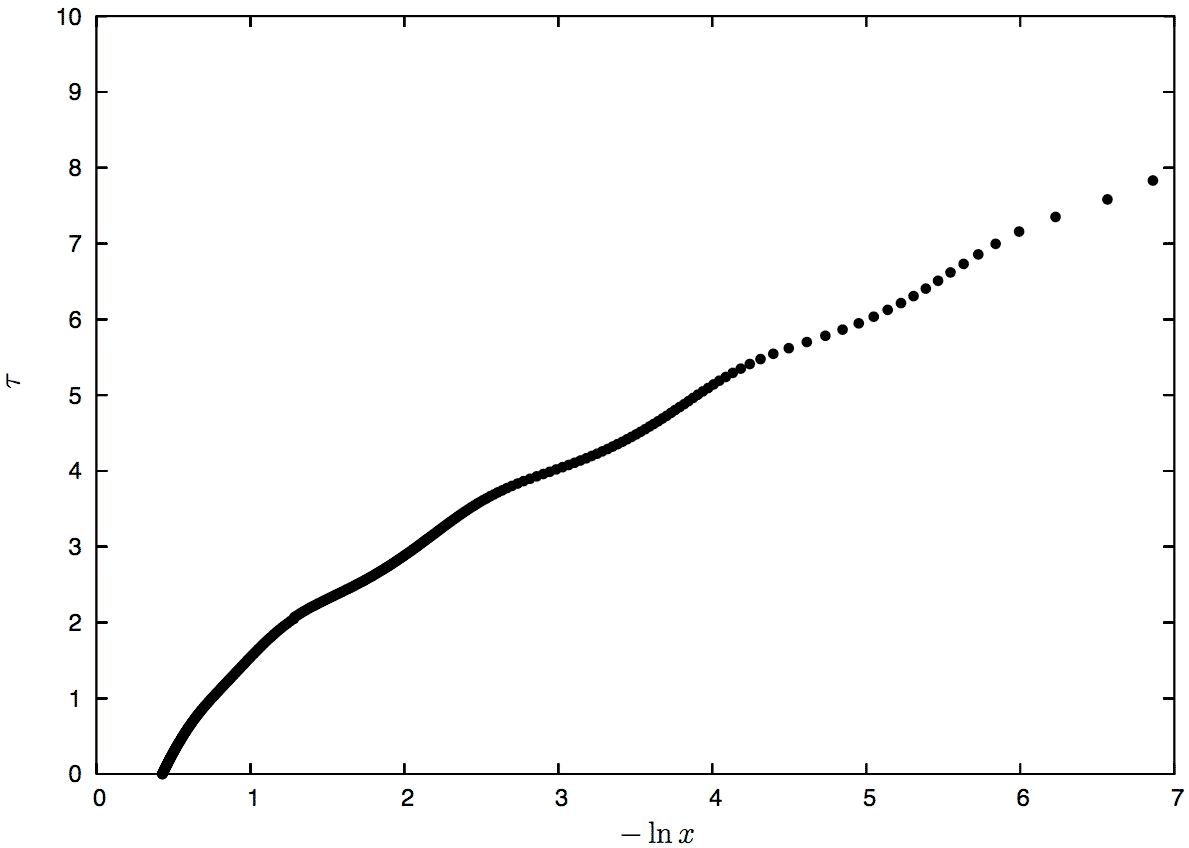
7.2 Results from the Double-Null Code
The results shown here are based on fine-tuning of Gaussian initial data
| (7.2.1) |
In section 7.2.4 we introduce double Gaussian data that are merely a superposition of two such Gaussians with parameters adjustable for each pulse.
7.2.1 Scaling
To complement the results from the DICE code, figures 7.18 and 7.19 show the expected scaling behavior for the black hole mass and the Ricci scalar curvature from a one-parameter family of evolutions generated by the double null code, respectively. According to its dimension being , the scalar curvature scales as , as discussed in section 5.3.
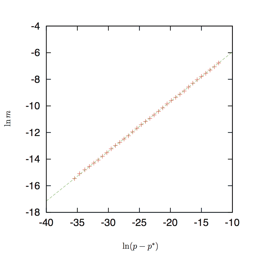
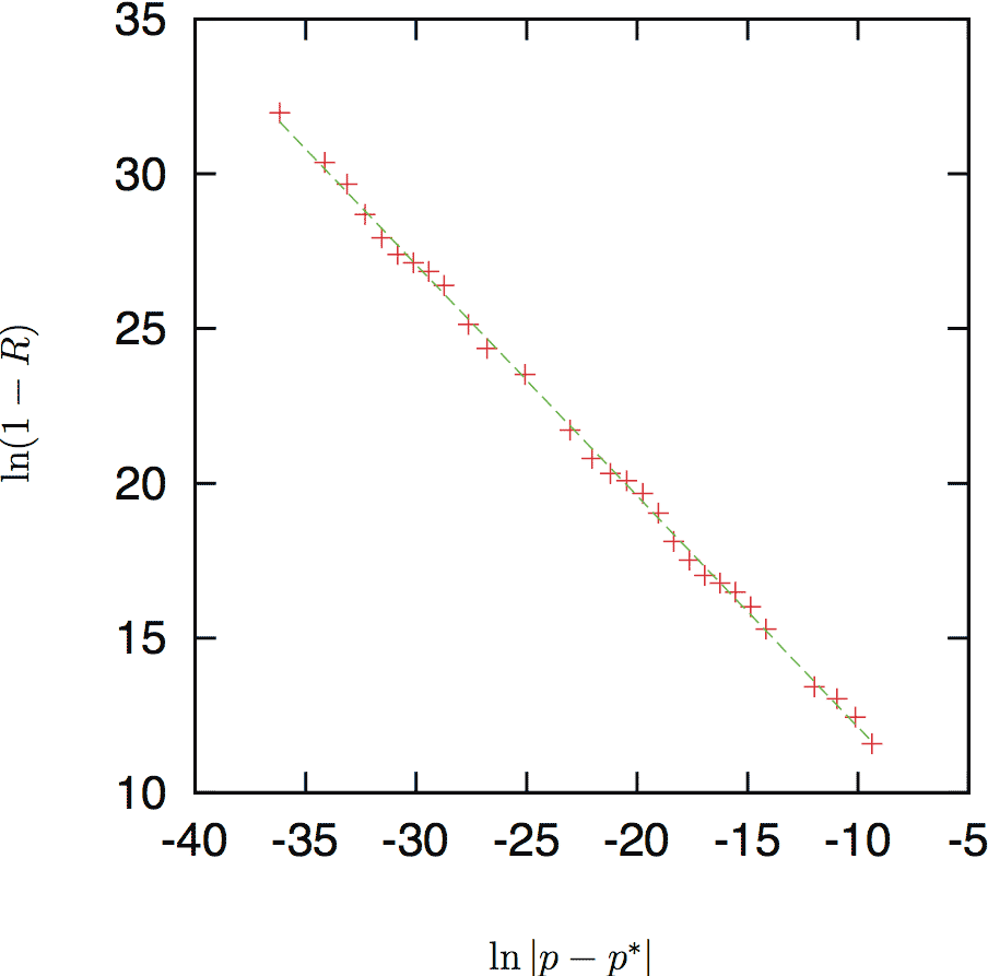
7.2.2 Horizons and
In section 7.1.2 we mentioned that exterior matter, , accumulates outside the past self-similarity horizon and we conjectured that, for late times, the mass originates from backscattering of outgoing radiation during the self-similar collapse. In a supercritical evolution, two scenarios are possible: Either eventually falls through the horizon, or it is radiated to infinity. In the former case, the resulting black hole will have a tiny but finite Bondi mass, no matter how fine tuned the data are, whereas, in the latter case, the Bondi mass can be made arbitrarily small.
We would like to explicitly verify whether this matter, , falls through the event horizon. (A compactified code that could penetrate apparent horizons would presumably still have to stop at the event horizon, due to reaching future timelike infinity, . Using an uncompactified code, we will have to settle for a reasonable local approximation of the event horizon.)
At first, it would seem that one could investigate the final fate of with any evolution code that can penetrate apparent horizons, such as the double null code of section 4.2. As it turns out, however, codes based on outgoing null slices are ill-suited to tackle this issue.
Only the immediate vicinity of the event horizon is relevant for the solution of this problem. Null slices too far to the future of the event horizon no longer contain , since the slices will have “bent” towards the curvature singularity at , and trapped gridpoints which come too close to the singularity will have been excised, as has been discussed in section 4.2.4. This leaves us with a slice where the very features we would like to study, namely the exterior matter, have probably already fallen into the singularity.
To illustrate the behavior of the mass function on outgoing null slices in the vicinity of apparent horizon formation we compare a series of slices for a near-critical evolution using 5000 gridpoints in figure 7.20. If a slice contains an apparent horizon, the function increases monotonically from the origin outwards until the locus of the AH is reached; there, it reverses direction and decreases monotonically until it reaches the singularity at . Gridpoints which come too close to the singularity must be excised. In contrast, figure 7.21 depicts a series of slices for a near-critical evolution which ultimately is subcritical. The two plots are superimposed in figure 7.22.
To improve the chance to observe the exterior mass falling into the horizon, it is clearly beneficial to decrease the timestep as far as possible. Unfortunately, the double null code relies on the condition for the approximation of derivatives close to the origin. We have tried to use interpolation to get rid of this condition, but our efforts introduced instabilities that made evolutions unusable. There is, in principle, another way. Namely, keep the condition and increase the overall spacetime resolution, i.e. both gridspacings. The result of such a brute force evolution using gridpoints is shown in figure 7.23. The horizon mass is almost two orders of magnitude lower, but the bending-over of the slices is still much too abrupt and all the exterior mass has been excised on the first slice which contains an apparent horizon in this evolution.
The behaviour discussed above is a deficiency intrinsic to our choice of slicing: Null-slices are inherently unstable near a horizon. Outgoing null-slices either extend till , if they are untrapped, or end at the singularity (with the exception of the event horizon which extends till ). Thus, it would be seem to be appropriate to use a Cauchy code to investigate this issue further. This would allow us to scan the horizon for exterior infalling matter.
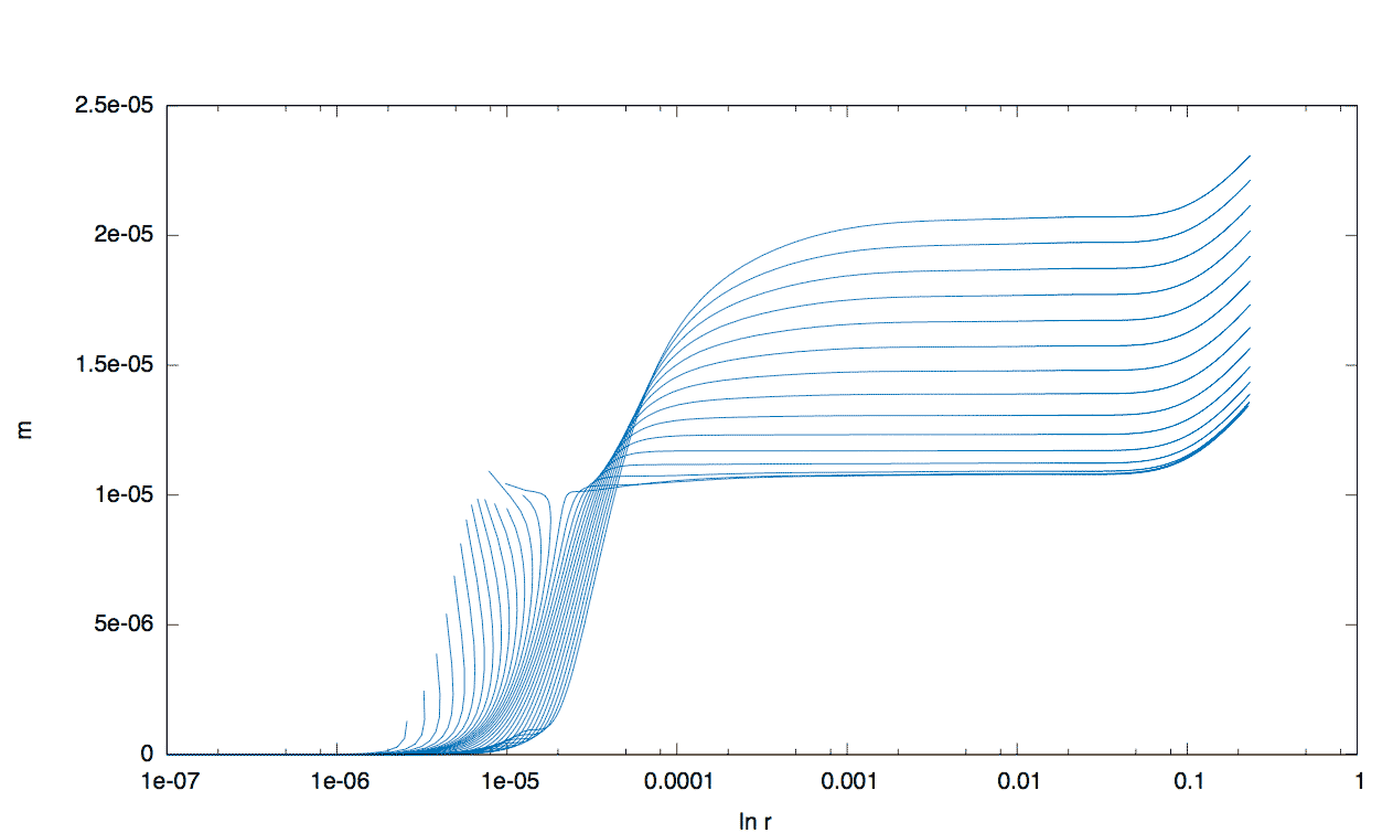
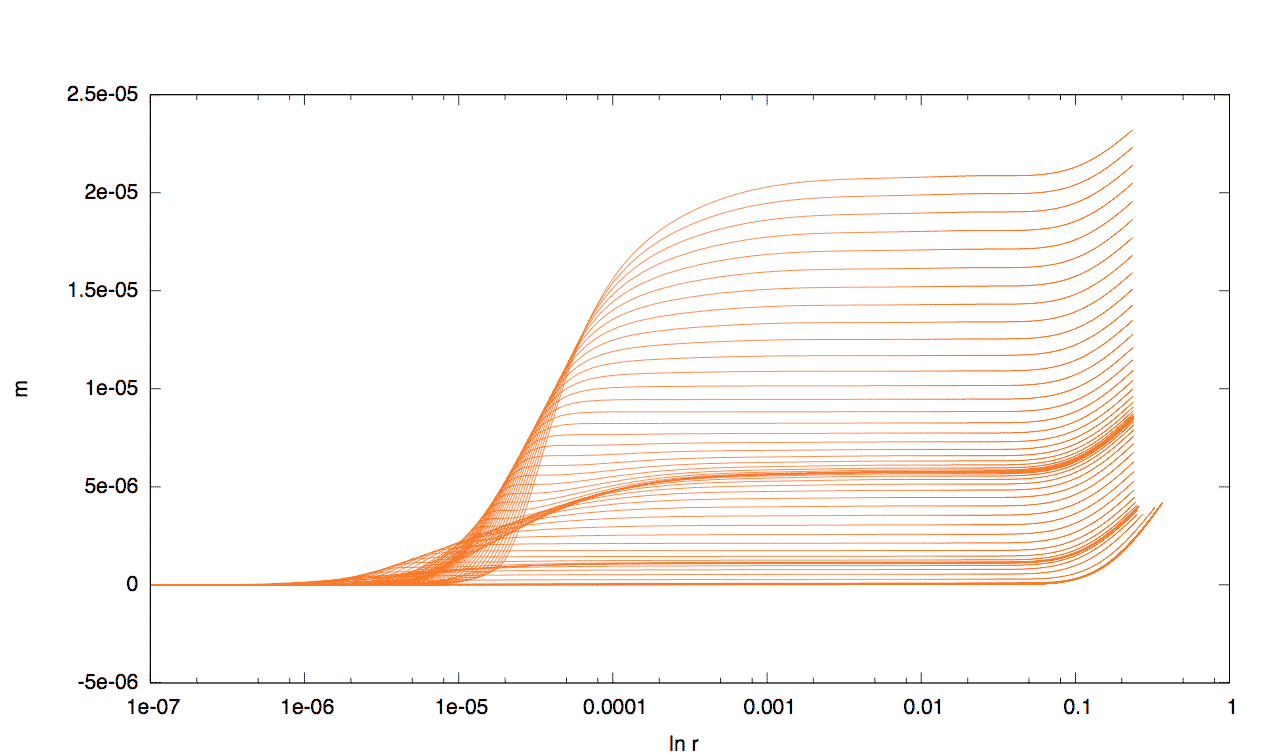

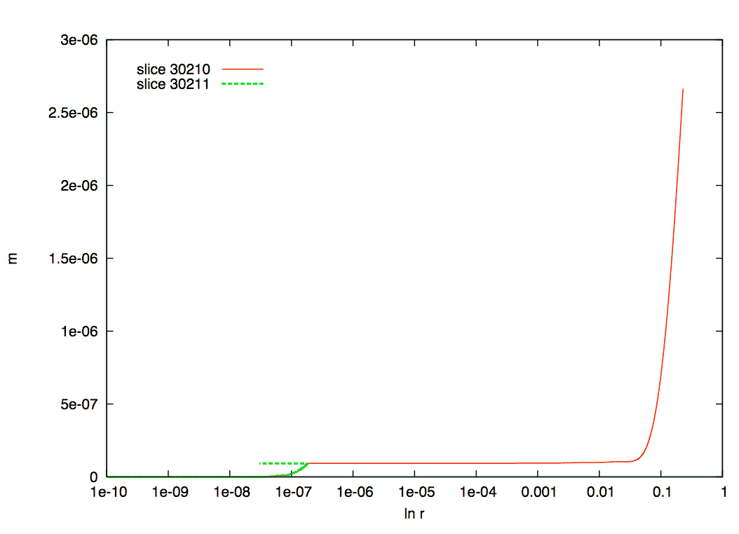
7.2.3 Dependency of on Initial Data
In the following, we would like to discuss the dependance of the exterior matter, , on the initial data. First, choose a family of initial data and fix all free parameters except for the parameter that will be used for fine-tuning. Within such a family, as we tune the parameter to criticality, we can reliably measure only if at some null slice in a given evolution, the interior mass is of the same order or smaller than or the interior and exterior mass are spatially well separated. In practise, this condition is only fulfilled at late times for very near-critical evolutions which severely restricts the interval in the initial data parameter and evolution time over which we can accurately measure the exterior mass .
From the analysis of a typical single near-critical (but supercritical) evolution, oscillates from the time we can first detect it until the last null slice before horizon formation, while the interior mass (contained in the past SSH) undergoes critical collapse and periodically sheds mass. If we instead consider a family of supercritical evolutions which become more and more near-critical, and measure at the last slice before horizon formation, roughly stays constant.
It is also important to note that, using generic (e.g. Gaussian) initial data, which have been fine-tuned, the solution evolves through a non-universal and family dependent stage before it approaches the self-similar regime. Since backscattering of radiation is already present in this initial stage, we expect to also depend on the shape or family of initial data used.
7.2.4 Double Gaussian Initial Data Results
In an effort to shed some light on the issue concerning the possible infall of the external mass , we have devised initial data to model this physical situation. Essentially, we are dealing with a near-critical evolution where the interior part is in the DSS regime (for a certain time) while further outside, there is another concentration of energy. Therefore, it is sensible to chose initial data which consists of two Gaussian pulses of scalar field, which we call double Gaussian initial data for short.
As it turns out, is not dense enough to form an apparent horizon by itself. This can be guessed from the fact that there is no apparent peak in at the locus of . It is also possible to evolve data that are based on the numerical scalar field solution on a null slice of a near-critical evolution where the presence of is the dominating contribution of mass. Using such a solution, , (preferably the last available slice before the formation of an AH) as new initial data is fairly straightforward. In is necessary to employ interpolation to obtain equally spaced initial data for the scalar field . Here, we have also had to fix the null gauge, which determines how the gridpoints are labeled by and . If necessary, taper the gridfunction such that the gradients in the interior part are smooth enough that they do not form trapped surfaces; in practise, this is taken care of automatically by the interpolation. We have carried out this procedure and found that the new spacetime is subcritical.
The accumulation of exterior mass that occurs naturally via backscattering in critical collapse could be modeled by data where the outer pulse is chosen weak enough so that it does not collapse by itself. Unfortunately, simulations of that type did not yield any new insights, since we still run into the problem of the bending-over of slices and forced excision of the part of the slice we would like to follow further.
Although not directly related to the issue we would like to solve, we have investigated spacetimes where the outer pulse can form a horizon, while the interior pulse evolves, more or less unaffected from the outer pulse, as they are interesting in their own right. In particular, we consider a configuration where the outer pulse froms an AH first (in retarded time ), while we can still follow the interior pulse in its critical collapse. Later (in retarded time), the interior pulse may itself form trapped surfaces, which creates a jump in the trapping horizon. A spacetime diagram of such an evolution is shown in figure 7.24. Figure 7.25 presents a density plot of for this evolution, (with a detail shown in figure 7.26), while figure 7.27 shows a perspective view.
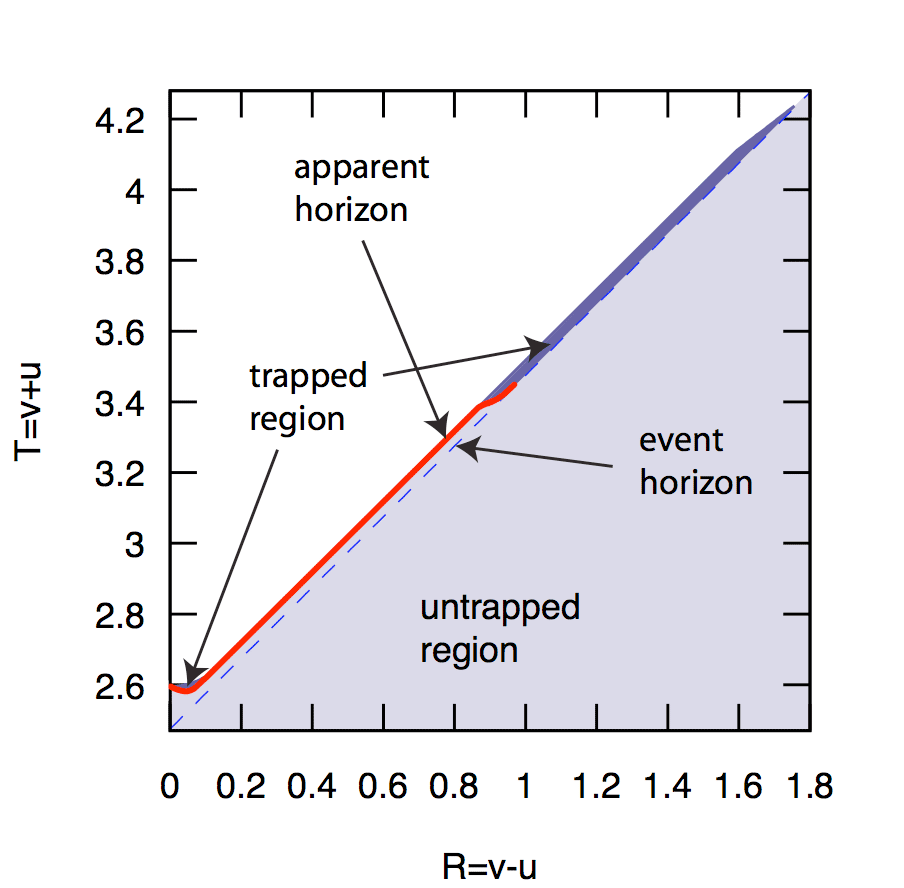

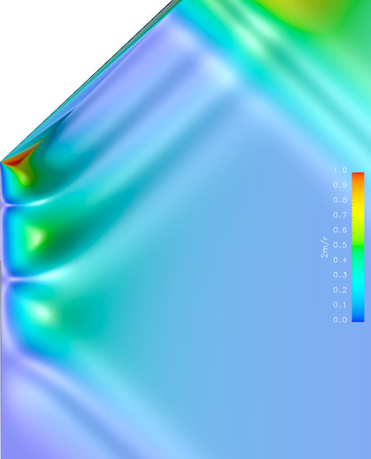
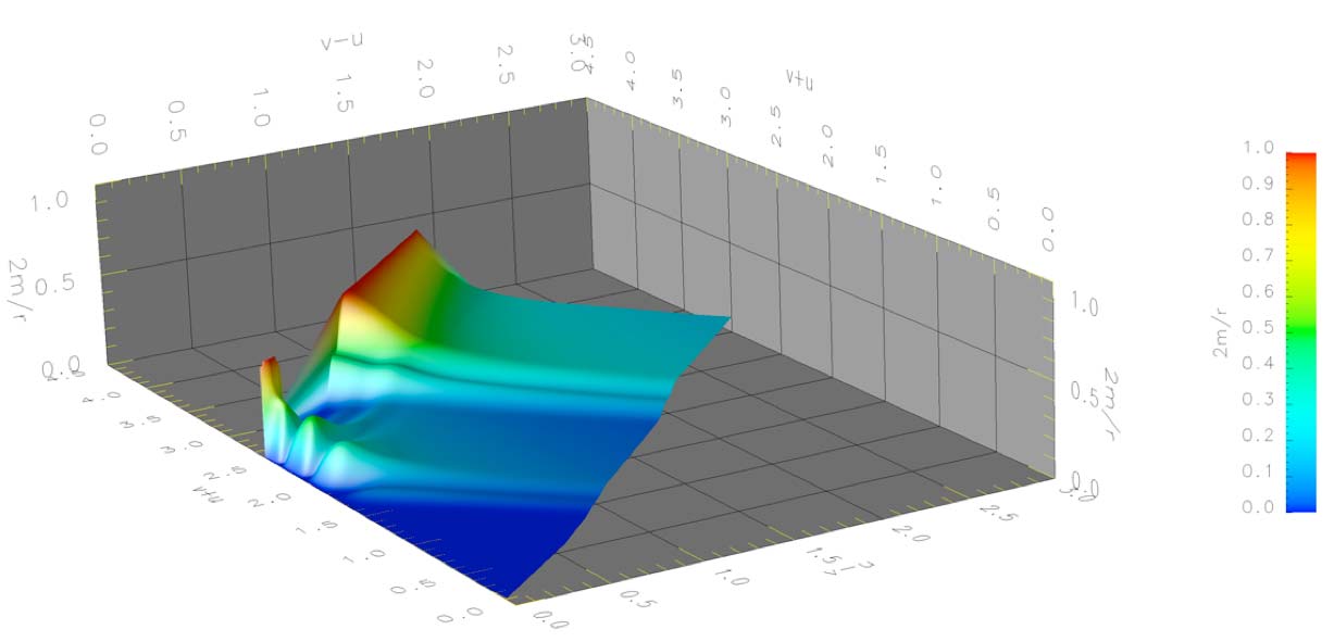
7.2.5 Timelike Observers and versus Diagrams
For timelike observers at we can compute the proper time as discussed in sections 3.8.3 and 4.2.7. In doing so, we obtain a grid on which we can display quantities of interest, such as the density function . Since this grid is neither orthogonal, nor equispaced, we need to resort to interpolation for some plots.
In order to have more resolution in the vicinity of the origin, one can use a static mapping in the distribution of the observers. A useful convex mapping is to equally space the observers in a computational coordinate and define with , so that . Figure 7.28 shows a color-coded density plot of on such a grid, where the null slices have been overlaid. Grid refinements are clearly visible when the density of the slices suddenly doubles. The geometry is initially flat. The evolution uses double Gaussian initial data, where the exterior pulse forms the first (in retarded time ) apparent horizon and the interior collapses at a later null slice after moving away from the DSS regime.

In contrast, figure 7.29 compares the fate of observers in a supercritical and a subcritical evolution.
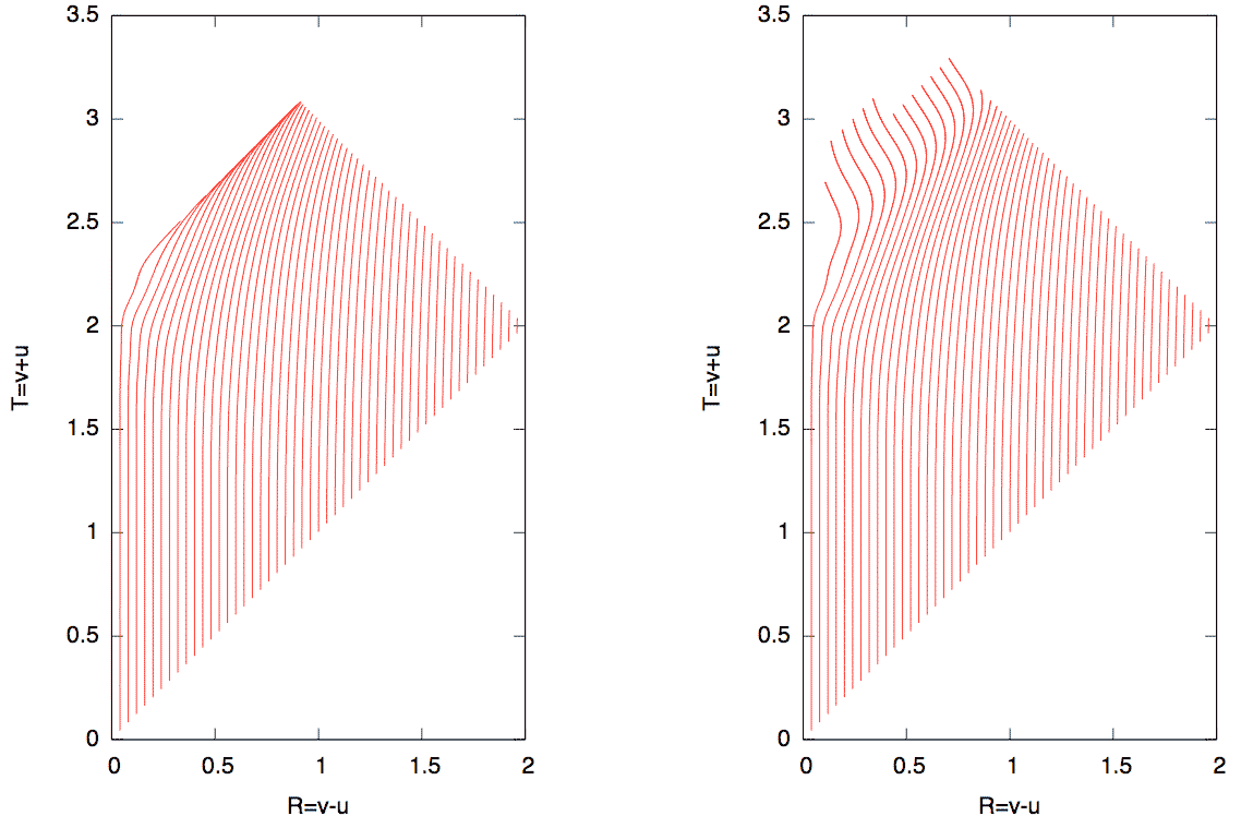
Chapter 8 Discussion
In this thesis we have presented numerical constructions of portions of near-critical spherically symmetric spacetimes that extend up to future null infinity. The simulations are based on a compactified approach, where the equations have been regularized in a neighborhood of null infinity by introducing the mass-function as an additional independent variable. Further simulations have been carried out using a double-null code that can penetrate apparent horizons. In this discussion, however, we focus on key results obtained from the compactified code as they represent the new developments in this thesis. The resolution necessary to resolve critical phenomena is gained through letting our gridpoints fall along ingoing null geodesics, following Garfinkle [Gar95]. The grid is repopulated with grid points, which are filled with values through interpolations when half of the gridpoints have reached the origin. This is not optimal, but ensures sufficient resolution for our current purposes.
We reproduce standard features of near-critical solutions, such as “echoing” and mass scaling with fine structure. The mass scaling law for compactified evolutions shows a “leveling-off” effect for very near-critical solutions that is not present for uncompactified simulations which we attribute to numerical errors. In addition, we extract radiation at null infinity by computing the news function and find a signal with rapidly increasing frequency as measured in Bondi time, which is the natural time coordinate associated with far away observers. In order to simplify the analysis of near-critical spacetimes, we have defined an approximate adapted time in terms of Bondi time, in analogy to the standard time coordinate which is adapted to the DSS discrete diffeomorphism (5.1.1). This coordinate can be used by asymptotic observers to render the signal from a near-critical collapse (almost) periodic. The fact that such a definition actually works out, and makes DSS periodicity manifest in quantities defined at null infinity is a non-trivial result, which we explain in Sec. 7.1.1.
Note also that the amplitude of the news function, shown in Fig. 7.1 stays fairly constant after the initial transient. This feature is clearly universal, as long as the radiation signal is dominated by the DSS collapse, since the system can be approximated in the DSS region by a perturbation of the critical solution. Thus, in section 7.1.2, we neglect contributions from scalar field which is far outside the DSS region and does not contribute to the critical collapse dynamics. Consequently, in this scenario the essential free parameters determining the radiation signal from an actual near critical solution are the number of cycles the solution spends in the neighborhood of the critical solution and the length scale (e.g. the “size” of the past SSH) at which the solution comes close to the critical solution. The robustness of this scenario, i.e. what happens if the initial data are such that there is significant mass outside of the SSH, is beyond the scope of this thesis and an issue for future research.
Perhaps the most surprising feature of the radiation signal has emerged from our investigation of QNMs, which has been motivated by [GPP94b], where the first quasinormal mode is found in collapse evolutions and the question is posed as to how QN ringing would change close to criticality. We find that even in very close-to-critical evolutions there is a correlation of the radiation signal with the period of the first quasinormal mode, determined from the time-dependent value of the Bondi mass, as discussed in Sec. 6.2, Figs. 6.1 and 6.2. This correlation between the radiation of the highly dynamical near-critical solution and the quasinormal mode, that is defined in terms of perturbations of a static spacetime, certainly deserves further investigation. This surprising feature might even turn out to be a key toward understanding the phenomenon of DSS behaviour in near-critical spacetimes. Our results seem to suggest that the effective curvature potential for a DSS self-gravitating field acts as a quasi-stationary background for scattering processes which can be approximately described by quasinormal modes of a one-parameter family of Schwarzschild black holes with exponentially decreasing mass.
This Schwarzschild background with decreasing mass can also be modeled by the Vaidya solution as discussed in section 6.3. Abdalla, Chirenti, and Saa [ACS06] have computed QNM for the Vaidya metric and have put forth a criterion to analyze whether a spacetime is in the “stationary adiabatic regime” where the real part of the QNM varies inversely with the mass function. We have been able to verify that our critical collapse evolutions are indeed in this stationary regime.
The question of the applicability of QNM-motivated estimates is quite relevant for numerical relativity, e.g. when extracting wave forms from binary mergers.
For subcritical initial data we can evolve for very long times, and thus are able to observe power-law tail behavior as shown in Figs. 6.7 and 6.8. Analytical calculations predict different falloff rates for radiation along null infinity and along timelike lines, and the natural question arises, which falloff rate would be seen by a hypothetical observer (in a realistic case, observation of power-law tails would require an extremely large signal-to-noise ratio). Accordingly, our results depicted in Fig. 6.7 show how the rates at finite but large radius correspond to the value for null infinity for a while before they approach the expected late-time value for finite radius. The interpretation of this phenomenon is suggested by perturbative work of [Bar99a, Bar99b], where different tail falloff rates are computed. There, different regions of spacetime are identified, where certain approximations hold. Within the perturbative regime, results obtained for null infinity are valid for what has been termed the “astrophysical zone” by Leaver [Lea86a, Lea86b, Bar99a], and which is defined as the region where . (Note, however, that must also be satisfied). The physical idea is that the distance from observers of astrophysical phenomena, e.g. gravitational wave detectors, to the radiation sources is very large compared to the time during which the source radiates at an observable rate.
We argue that our results illustrate that the relevant falloff from the point of view of an astrophysical observer is the falloff rate at null infinity, in accordance with the prediction from perturbation theory. We believe that this is a nice model calculation that exemplifies that null infinity is indeed a useful approximation for observers at large distance from the source, in the sense that such observers are located in the “astrophysical zone”.
Along the same lines, we would like to point out that by taking appropriate limits in a conformally compactified manifold, worldlines of increasingly distant geodesic observers converge to null geodesic generators of future null infinity and proper time converges to Bondi time [Fra00]. Note also that a naive correspondence between observers at large distance and spatial infinity would be problematic, e.g. compactification at spatial infinity leads to “piling up” of waves, whereas at null infinity this effect does not appear – waves leave the physical spacetime through the boundary at null infinity.
Under practical circumstances, null infinity more realistically corresponds to an observer that is sufficiently far away from the source to treat the radiation linearly, but not so far away that cosmological effects have to be taken into account. We are however not aware of a discussion where this sloppy picture has been made more precise.
When looking at critical collapse from a global spacetime perspective, as we have done here, one is confronted with some issues concerning the mass-scaling, that we would like to comment on briefly: When asking the question of whether infinitesimally small black holes can be formed – the question which triggered the original work on critical collapse – it could be phrased in two slightly different ways: (i) can we form black-hole solutions where the final-state black hole has arbitrarily small mass, or (ii) can we form arbitrarily small apparent horizons. The question which has been answered in the affirmative by critical collapse research is the second one. The first one still seems open. Our results for near-supercritical evolutions indicate that the mass outside the past self-similarity horizon, is significantly larger than the mass leading to scaling. We conjecture that this external mass originates from backscattering of outgoing radiation. If this mass falls into the black hole, then, clearly, one cannot form arbitrarily small black holes, no matter how fine-tuned the data are.
The application of a double-null code that can penetrate apparent horizons has not been able to decide whether the exterior matter really falls through the horizon; instead of a null slicing, which has proven inherently unstable close to the event horizon, we propose to use a Cauchy evolution code for future work.
Considering the observability of critical collapse from future null infinity in an astrophysical context, one might first object that the matter model discussed here is unphysical. On the one hand, it was chosen for mathematical simplicity. On the other hand, the curved space wave equation of the simple scalar field model still shares some essential nonlinear features inherent in the full Einstein equations without symmetry. Moreover, it would be possible to remedy this deficiency by using e.g. a perfect fluid or gravitational waves in axisymmetry. A much more serious problem is the high degree of finetunedness required in the initial data to develop sufficient self-similar features in spacetime such that they could be detected by far away observer.
Chapter A Tensor Components in Bondi Coordinates
| (A.0.1) | ||||
| (A.0.2) | ||||
| (A.0.3) | ||||
| (A.0.4) | ||||
| (A.0.5) |
| (A.0.7) |
| (A.0.8) | ||||
| (A.0.9) | ||||
| (A.0.10) | ||||
| (A.0.11) | ||||
| (A.0.12) |
Energy momentum tensor of a massless scalar field
| (A.0.14) | ||||
| (A.0.15) | ||||
| (A.0.16) | ||||
| (A.0.17) | ||||
| (A.0.18) | ||||
| (A.0.19) |
| (A.0.21) |
Curved space wave equation (matter field equation)
| (A.0.22) |
Christoffel symbols
| (A.0.23) | ||||
| (A.0.24) | ||||
| (A.0.25) | ||||
| (A.0.26) | ||||
| (A.0.27) | ||||
| (A.0.28) | ||||
| (A.0.29) | ||||
| (A.0.30) | ||||
| (A.0.31) | ||||
| (A.0.32) | ||||
| (A.0.33) | ||||
| (A.0.34) |
Chapter B Tensor Components in Double Null Coordinates
Einstein Tensor
| (B.0.1) | ||||
| (B.0.2) | ||||
| (B.0.3) | ||||
| (B.0.4) | ||||
| (B.0.5) |
Christoffel symbols
| (B.0.6) | ||||
| (B.0.7) | ||||
| (B.0.8) | ||||
| (B.0.9) | ||||
| (B.0.10) | ||||
| (B.0.11) | ||||
| (B.0.12) | ||||
| (B.0.13) | ||||
| (B.0.14) | ||||
| (B.0.15) | ||||
| (B.0.16) | ||||
| (B.0.17) |
Chapter C Numerical Methods
C.1 Finite Difference Methods for ODEs
Following [AP98], we consider numerical solutions to the initial value problem (IVP)
| (C.1.1) |
on a mesh
| (C.1.2) |
and let the nth step size. We assume sufficient smoothness and boundedness on so that a unique solution exists and has as many bounded derivatives as required. Let be the mesh function which takes on the value at each , where the denote approximations to the exact solution .
For the sake of simplicity, consider the forward Euler method,
| (C.1.3) |
We define the difference operator of the forward Euler method as
| (C.1.4) |
for some function defined at the mesh points. Then, represents the discretized form of the ODE (C.1.1). The local truncation error (LTE) (or local discretization error) 111 This definition of the local truncation error can also be interpreted as the error generated by a single numerical step starting from exact data and dividing the result by : i.e. for the forward Euler method denote the result of this step by . Then . In contrast to this definition, the LTE is often defined by . is the residual of the difference operator when it is applied to the exact solution:
| (C.1.5) |
The difference method is said to be consistent (or accurate) of order if
| (C.1.6) |
for a positive integer . For the forward Euler method we have
| (C.1.7) |
thus, it is consistent of order 1.
We define the global error
| (C.1.8) |
and assume that . Let and assume that is bounded independent of . The difference method is said to be convergent of order if the global error, , satisfies
| (C.1.9) |
for .
Theorem 3.1 of [AP98] states that: If a numerical method is consistent of order and fulfills a certain concept of stability (“0-stability” 222 A difference method is called 0-stable if there exist positive constants and such that for any mesh functions and with , ), then it is convergent of order .
In contrast to the local truncation error, the local error is defined as the amount by which the numerical solution at each timestep differs from the solution to the initial value problem
| (C.1.10) |
The local error is defined by
| (C.1.11) |
For the numerical methods we consider here, the local error indicators and are closely related:
| (C.1.12) |
C.2 Runge Kutta Methods
We discuss the Runge-Kutta methods [AP98] used to solve ODEs in our numerical codes. Runge-Kutta methods belong to the class of one-step methods, i.e methods that do not use any information from previous steps. In a typical step of size , we seek an approximation to , given the result of the previous step, .
Given the scalar initial value problem
| (C.2.1) |
we can approximate the area under the curve by applying one of the quadrature rules given in section C.2.1 to the integral in
| (C.2.2) |
on a mesh
| (C.2.3) |
and let the nth step size. For instance, we can use the height at the midpoint of the interval, i.e. , where . This choice leads to the implicit midpoint method
| (C.2.4) |
Approximating by the forward Euler method we obtain the explicit midpoint method:
| (C.2.5) | ||||
| (C.2.6) |
According to equation (C.1.6), both midpoint methods have a local truncation error of and are consistent of order 2.
Applying the trapezoidal rule to C.2.2 yields the implicit trapezoidal method
| (C.2.7) |
To obtain an explicit method, we approximate using the forward Euler method, which yields
| (C.2.8) | ||||
| (C.2.9) |
This is an explicit 2-stage method of order 2, known as the explicit trapezoidal method.
C.2.1 Quadrature Rules
For the sake of reference we list some very well known approximations to the integral and their global errors:
-
•
Midpoint-Rectangle rule:
(C.2.10) -
•
Trapezoidal rule:
(C.2.11) -
•
1/3 Simpson’s rule:
For the subinterval :(C.2.12) while for the entire interval
(C.2.13) where is even.
C.3 Error Analysis of the NSWE-algorithm
C.3.1 Local Errors
The local errors in the NSWE-scheme (3.5.2) of section 3.5 stem from the approximation of the integral by evaluating the integrand at the center of the small null parallelogram (see figure C.1) and from the multiplication with the area of this diamond-shaped region. Evaluating the integrand at the center amounts to the same as using the average between the points and .
Assume that we know a function at the endpoints and of a given interval (see figure C.2) and want to evaluate it at the midpoint of the interval . Using linear interpolation at the center of an interval we find
| (C.3.1) |
The approximation error for the linear interpolation polynomial with pairwise distinct nodes is (see [DH03])
| (C.3.2) |
for some . Therefore, this polynomial approximation is second order accurate.
The approximation of the integral in (3.5.2) applies the midpoint-rule to the integrand which is multiplied by the area which is of the order . (If , then .) Since both factors are second order accurate, the local error of one NSWE-integration step is , assuming that , and are known at least to this order.
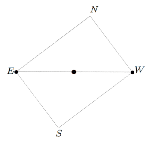
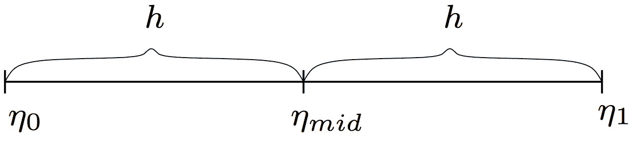
C.3.2 Global Errors
In the following, we give a heuristic argument for the global error of the NSWE-scheme. First, we restrict analysis to the fixed background case. This entails that the NSWE-scheme is no longer coupled to the geometry and null-geodesic ODEs, which would in general have to be solved concurrently. To simplify matters even more, we discard the Taylor expansion-region and use just as a startup condition. Note that for flat space the algorithm is exact, since .
The general idea is the following: We start out from the initial slice where is known exactly. On the next slice, we march outwards from the origin using the NSWE-algorithm whose computational molecule is shown in figure C.3 and accumulate local error terms of order as illustrated in figure C.4. If we make steps and we will loose one order of accuracy. On the next slice, however, we are still using -values of order near the origin. In a Cauchy code we would accumulate errors only along the time direction. Here, we can distinguish two directions of error accumulation: one radially outward and another along the ingoing null-geodesics. Thus, we loose two orders in total and the diamond algorithm turns out to be globally second order accurate:
| (C.3.3) |
For the coupled NSWE-algorithm one has to choose the orders of accuracy for the ODE solvers such that the diamond scheme stays globally second order accurate. In practise, second order accurate schemes (see C.2) have proven sufficient to ensure this.
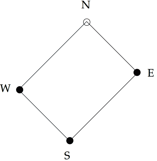
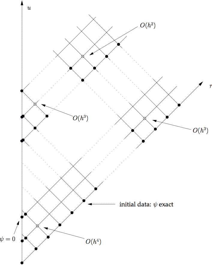
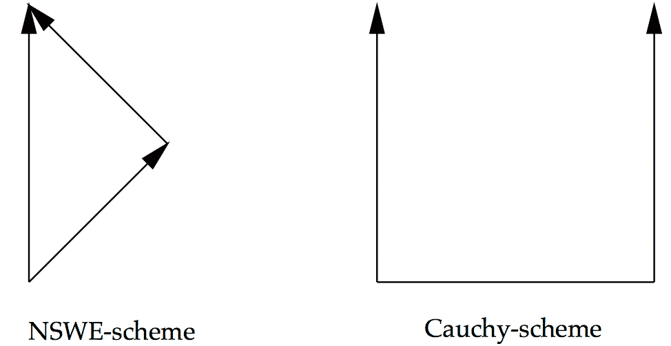
Chapter D Convergence Test Methodology
We briefly describe how we can check the accuracy of a numerical evolution code using the concept of convergence tests. These tests obtain error estimates by subtracting numerical solutions on a grid which is shared by a set of evolutions using different (usually by powers of two) gridspacings. Depending on whether the quantities to be tested are zero on the continuum level or not, we take one of the following approaches:
In a so-called 3-level convergence test, we use three different grid resolutions, with n being the number of gridpoints in the lowest resolution grid, and the higher ones having and gridpoints, respectively. Without restriction of generality, we can assume that the gridspacing on a grid of gridpoints is given by . Assume furthermore that the discretized field is second order accurate,
| (D.0.1) |
where the continuum error functions and do not depend on the gridspacing . Then,
| (D.0.2) | ||||
| (D.0.3) |
We may subtract these gridfunctions on the common gridpoints,
| (D.0.4) |
and
| (D.0.5) |
Comparing the last two expressions we find that on the coarsest grid
| (D.0.6) |
By taking a discrete spatial norm over the grid, we can compute a time-dependent convergence factor
| (D.0.7) |
If the numerical scheme converges, then in the limit we should find
| (D.0.8) |
In general we have, for ,
| (D.0.9) |
where denotes the exponent of the leading error term in the discretized field and the factor between grid resolutions.
A 2-level convergence test is applicable to discretized quantities that are supposed to be zero on the continuum level, i.e.
| (D.0.10) |
It then follows that
| (D.0.11) |
More generally we have, for ,
| (D.0.12) |
References
- [ACS06] Elcio Abdalla, Cecilia B. M. H. Chirenti, and Alberto Saa. Quasinormal modes for the Vaidya metric. Phys. Rev. D, 74(084029), 2006.
- [AG05] Miguel Alcubierre and José A. González. Regularization of spherically symmetric evolution codes in numerical relativity. Comput. Phys. Commun., 167:76–8, 2005.
- [AK02] A. Ashtekar and B. Krishnan. Dynamical horizons: Energy, angular momentum, fluxes, and balance laws. Phys. Rev. Lett., 89:261101, 2002.
- [AK03] A. Ashtekar and B. Krishnan. Dynamical horizons and their properties. Phys. Rev. D, 68:104030, 2003.
- [AK04] A. Ashtekar and B. Krishnan. Isolated and dynamical horizons and their applications. Living Reviews in Relativity, 7(10), 2004.
- [AMS05] Lars Andersson, Marc Mars, and Walter Simon. Local existence of dynamical and trapping horizons. Phys. Rev. Lett., 95(111102), 2005.
- [And02] Lars Andersson. Construction of hyperboloidal initial data. Lect. Notes Phys., 604:183–194, 2002.
- [AP98] Uri M. Ascher and Linda R. Petzold. Computer Methods for Ordinary Differential Equations and Differential-Algebraic Equations. Society for Industrial and Applied Mathematics, 1998.
- [Bar99a] Leor Barack. Late time dynamics of scalar perturbations outside black holes. I. A shell toy model. Phys. Rev. D, 59:044016, 1999.
- [Bar99b] Leor Barack. Late time dynamics of scalar perturbations outside black holes. II. Schwarzschild geometry. Phys. Rev. D, 59:044017, 1999.
- [Biz96] P. Bizoń. How to make a tiny black hole? Acta Cosmologica, 22:81, 1996.
- [BM88] Robert Bartnik and John McKinnon. Particlelike solutions of the Einstein-Yang-Mills equations. Phys. Rev. Lett., 61:141, 1988.
- [BO84] Marsha J. Berger and Jospeh E. Oliger. Adaptive mesh refinement for hyperbolic partial differential equations. Journal of Computational Physics, 53:484–512, 1984.
- [BP83] James M. Bardeen and Tsvi Piran. General relativistic axisymmetric rotating systems: Coordinates and equations. Physics Reports (Review Section of Physics Letters), 96(4):205–250, 1983.
- [CH62] Richard Courant and David Hilbert. Methods of Mathematical Physics, Partial Differential Equations, volume II. Interscience Publishers, John Wiley & Sons, 1962.
- [Cha83] S. Chandrasekhar. The Mathematical Theory of Black Holes. Clarendon Press, Oxford, 1983.
- [Cho93] Matthew W. Choptuik. Universality and scaling in gravitational collapse of a massless scalar field. Physical Review Letters, 70:9–12, 1993.
- [Cho98] Matthew W. Choptuik. The (unstable) threshold of black hole formation. In N. Dadhich and J. Narlikar, editors, Proceedings of the GR-15 Conference in Pune, pages 67–85, 1998.
- [Chr86] D. Christodoulou. The problem of a self-gravitating scalar field. Commun. Math. Phys., 105:337–361, 1986.
- [Chr87] D. Christodoulou. A mathematical theory of gravitational collapse. Comm. Math. Phys., 109:613, 1987.
- [Chr91] D. Christodoulou. The formation of black holes and singularities in spherically symmetric gravitational collapse. Commun. Pure Appl. Math., 44:339–373, 1991.
- [Chr94] D. Christodoulou. Examples of naked singularity formation in the gravitational collapse of a scalar field. Ann. Math., 140:607–653, 1994.
- [Chr99] D. Christodoulou. The instability of naked singularities in the gravitational collapse of a scalar field. Ann. Math., 149:183–217, 1999.
- [DH03] Peter Deuflhard and Andreas Hohmann. Numerical Analysis in Modern Scientific Computing. Number 43 in Texts In Applied Mathematics. Springer, second edition edition, 2003.
- [d’I92a] R. A. d’Inverno, editor. Approaches To Numerical Relativity, 1992.
- [d’I92b] Ray d’Inverno. Introducing Einstein’s Relativity. Clarendon Press, Oxford, 1992.
- [FN98] Valery P. Frolov and Igor D. Novikov. Black Hole Physics, Basic Concepts and New Developments. Kluwer Academic Publishers, 1998.
- [Fra00] J. Frauendiener. Numerical treatment of the hyperboloidal initial value problem for the vacuum Einstein equations. III. On the determination of radiation. Class. Quant. Grav., 17:373, 2000.
- [Fra04] Jörg Frauendiener. Conformal infinity. Living Rev. Relativity, 7, 2004.
- [Fri81] Helmut Friedrich. The asymptotic characteristic initial value problem. Proc. R. Soc. London Sect. A, 378:401–421, 1981.
- [Gar64] P. R. Garabedian. Partial Differential Equations. John Wiley & Sons, Inc., 1964.
- [Gar95] David Garfinkle. Choptuik scaling in null coordinates. Phys.Rev. D, 51:5558–5561, 1995.
- [GD98] David Garfinkle and G. Comer Duncan. Scaling of curvature in subcritical gravitational collapse. Phys. Rev. D, 58(6):064024, 1998.
- [GP87] Dalia S. Goldwirth and Tsvi Piran. Gravitational collapse of massless scalar field and cosmic censorship. Physical Review D, 36(12):3575–3581, December 1987.
- [GPP94a] Carsten Gundlach, Richard H. Price, and Jorge Pullin. Late-time behavior of stellar collapse and explosions. I. Linearized perturbations. Phys. Rev. D, 49:883 – 889, 1994.
- [GPP94b] Carsten Gundlach, Richard H. Price, and Jorge Pullin. Late-time behavior of stellar collapse and explosions. II. Nonlinear evolution. Phys. Rev. D, 49:890 – 899, 1994.
- [GS04] Fernando Girotto and Alberto Saa. Semianalytical approach for the Vaidya metric in double-null coordinates. Phys. Rev. D, 70(084014), 2004.
- [Gun95] Carsten Gundlach. Choptuik spacetime as an eigenvalue problem. Phys. Rev. Lett., 75:3214, 1995.
- [Gun97a] Carsten Gundlach. Echoing and scaling in Einstein-Yang-Mills critical collapse. Phys. Rev. D, 55:6002 – 6013, 1997.
- [Gun97b] Carsten Gundlach. Understanding critical collapse of a scalar field. Phys. Rev. D, 55:695 – 713, 1997.
- [Gun98] Carsten Gundlach. Critical phenomena in gravitational collapse (review paper). Adv. Theor. Math. Phys, 2(1), 1998.
- [Gun99] Carsten Gundlach. Critical phenomena in gravitational collapse. Living Reviews in Relativity, http://www.livingreviews.org, 2, December 1999.
- [GW81] Robert Geroch and Jeffrey Winicour. Linkages in general relativity. Journal of Mathematical Physics, 22(4):803–812, April 1981.
- [GW92a] R. Gómez and J. Winicour. Gravitational wave forms at finite distances and at null infinity. Phys. Rev. D, 45:2776 – 2782, 1992.
- [GW92b] Roberto Gomez and Jeffrey Winicour. Asymptotics of gravitational collapse of scalar waves. Journal of Mathematical Physics, 33(4):1445–1457, April 1992.
- [GW92c] Roberto Gomez and Jeffrey Winicour. Numerical asymptotics. In Ray d’Inverno, editor, Approaches to Numerical Relativity, pages 143–162. Cambridge University Press, Cambridge (UK), 1992. Proceedings of the International Workshop on Numerical Relativity, Southampton University (Southampton, England), 16–20 December 1991.
- [GWS94] R. Gómez, J. Winicour, and B. G. Schmidt. Newman-penrose constants and the tails of self-gravitating waves. Phys. Rev. D, 49:2828 – 2836, 1994.
- [Har05] B. J. Carr Harada, T. Growth of primordial black holes in a universe containing a massless scalar field. Phys. Rev. D, 71:104010, 2005.
- [Hay94a] Sean A. Hayward. General laws of black-hole dynamics. Physical Review D, 49(12):6467–6474, June 1994.
- [Hay94b] Sean A. Hayward. Quasilocal gravitational energy. Physical Review D, 49(2):831–839, January 15 1994.
- [Hay96] Sean A. Hayward. Gravitational energy in spherical symmetry. Physical Review D, 53(4):1938–1949, February 1996.
- [HB62] A. Metzner H. Bondi, M. Van der Burg. Gravitational waves in general relativity VII. Waves from axi-symmetric isolated systems. Proc. R. Soc. London A269, 21, 1962.
- [HE73] S.W. Hawking and G.F.R. Ellis. The large scale structure of space-time. Cambridge University Press, 1973.
- [HLP+00] Sascha Husa, Christiane Lechner, Michael Pürrer, Jonathan Thornburg, and Peter C. Aichelburg. Type II critical collapse of a self-gravitating nonlinear model. Physical Review D, 62:104007, 2000.
- [HP97] Shahar Hod and Tsvi Piran. Fine-structure of Choptuik’s mass-scaling relation. Phys. Rev. D, 55:R440 – R442, 1997.
- [HS96] Rufus S. Hamade and John M. Stewart. The spherically symmetric collapse of a massless scalar field. Class. Quantum Grav., 1996.
- [HSVZ05] Sascha Husa, Carsten Schneemann, Tilman Vogel, and Anil Zenginoglu. Hyperboloidal data and evolution. In To appear in Proceedings of the 2005 spanish relativity meeting, AIP Conference Proceedings, 8 pages., 2005.
- [Hus07] Sascha Husa. personal communication, 2007.
- [Iye87] Sai Iyer. Black-hole normal modes: A WKB approach. II. Schwarzschild black holes. Phys. Rev. D, 35:3632 – 3636, 1987.
- [KHA95] T. Koike, T. Hara, and S. Adachi. Critical behavior in gravitational collapse of radiation fluid: A renormalization group (linear perturbation) analysis. Phys. Rev. Lett., 74:5170, 1995.
- [KS99] K. D. Kokkotas and B. G. Schmidt. Quasi-normal modes of stars and black holes. Living Reviews in Relativity, 2(2), 1999.
- [Kur84] Yuhji Kuroda. Naked singularities in the Vaidya spacetime. Prog. Theo. Phys., 72(1):63–72, 1984.
- [Lea86a] E. Leaver. J. Math. Phys., 27:1238, 1986.
- [Lea86b] Edward W. Leaver. Spectral decomposition of the perturbation response of the Schwarzschild geometry. Phys. Rev. D, 34:384 – 408, 1986.
- [Lec01] Christiane Lechner. Staticity, Self-Similarity and Critical Phenomena in a Self-Gravitating Nonlinear -model. PhD thesis, Universität Wien, 2001.
- [LTHA02] Christiane Lechner, Jonathan Thornburg, Sascha Husa, and Peter C. Aichelburg. New transition between discrete and continuous self-similarity in critical gravitational collapse. Phys. Rev. D, 65:081501, 2002.
- [Mai96] Dieter Maison. Nonuniversality of critical behavior in spherically symmetric gravitational collapse. Physical Letters B, 366:82–84, 1996.
- [MS64] Charles W. Misner and David H. Sharp. Relativistic equations for adiabatic, spherically symmetric gravitational collapse. Physical Review B, 136(2):571–576, October 26 1964.
- [NF89] Igor D. Novikov and Valery P. Frolov. Physics of Black Holes. Kluwer Academic Publishers, 1989.
- [NP62] E.T. Newman and R. Penrose. An approach to gravitational radiation by a method of spin coefficients. J. Math. Phys., 3(3):566–578, 1962.
- [NP68] E. T. Newman and R. Penrose. New conservation laws for zero rest-mass fields in asymptotically flat space-time. Proc. Roy. Soc., A. 305:175–204, 1968.
- [Pap74] Achille Papapetrou. Lectures on General Relativity. D. Reidel Publishing Company, 1974.
- [PHA05] Michael Pürrer, Sascha Husa, and Peter C. Aichelburg. News from critical collapse: Bondi mass, tails, and quasinormal modes. Phys.Rev. D, 71(10):104005, 2005.
- [PL04] Frans Pretorius and Luis Lehner. Adaptive mesh refinement for characteristic codes. J.Comp.Phys., 198:10–34, 2004.
- [Poi04] Eric Poisson. A Relativist’s Toolkit. Cambridge University Press, 2004.
- [Pri72] Richard H. Price. Nonspherical perturbations of relativistic gravitational collapse. I. Scalar and gravitational perturbations. Phys. Rev. D, 5:2419 – 2438, 1972.
- [Wal84] Robert M. Wald. General Relativity. University of Chicago Press, Chicago, 1984.
- [Win05] Jeffrey Winicour. Characteristic evolution and matching. Living Reviews in Relativity, 8(10):39, March 2005.
- [WR05] Inc. Wolfram Research. Mathematica Edition: Version 5.2. Wolfram Research, Inc., Champaign, Illinois, 2005.