Blowups of Heterotic Orbifolds using Toric Geometry

Abstract

Heterotic orbifold models are promising candidates for models with MSSM like spectra. But orbifolds only correspond to a special place in moduli space, the bigger picture is described by the moduli space of Calabi-Yau spaces. In this talk we will make explicit connections between both points of view. To this end we study blowups of orbifold singularities using both explicit constructions and toric geometry techniques. We show that matching of all orbifold models in blowups are possible.

1 Introduction and summary

One of the central aims of string phenomenology is to build string models reproducing the supersymmetric standard model of particle physics. There have been various approaches in this direction: Free–fermion models Faraggi:1989ka ; Faraggi:1991jr , intersecting D–branes in type II string theory Berkooz:1996km ; Blumenhagen:2000wh ; Aldazabal:2000dg ; Honecker:2004kb , Gepner models Dijkstra:2004cc ; Dijkstra:2004ym , and compactifications of the heterotic string. In the latter case in order to obtain at most four dimensional $N=1$ supersymmetry one needs to compactify on a Calabi–Yau space Candelas:1985en (for recent progresses see Andreas:1999ty ; Braun:2005bw ; Blumenhagen:2005zg ; Blumenhagen:2006ux ). Orbifolds (singular limits of Calabi–Yaus) are convenient, because they allow for calculable string compactifications dixon_85 ; Dixon:1986jc . It is possible to produce a vast but controllable landscape of models, and scan among them for realistic ones. Indeed, this approach has been proven to be successful, and models close to the MSSM have been built Forste:2004ie ; Kobayashi:2004ya ; Kobayashi:2004ud ; Buchmuller:2004hv ; Lebedev:2006kn ; Kim:2006hw .

Orbifolds are special points in the full moduli space of the heterotic string on Calabi–Yau manifolds. In order to have control on the theory away from these special points, it is crucial to have a better understanding of model building on the corresponding smooth compactification spaces. A concrete way to probe the moduli space surrounding orbifold points is to consider blowups of orbifold singularities. The construction of explicit blowups is unfortunately not easy. The best known example is the Eguchi–Hanson resolution Eguchi:1978xp of the $\mathbb{C}^{2}/\mathbb{Z}_{2}$ orbifold singularity. Generalization to $\mathbb{C}^{n}/\mathbb{Z}_{n}$ was discussed in Calabi:1979 . The singularities of more complicated orbifolds might not allow for a simple explicit blowup construction. On the other hand, the topological properties of such resolutions can be conveniently described by toric geometry, see e.g. Erler:1992ki .

In this talk we explain how using both explicit blowups and toric geometry one can construct heterotic models on orbifold resolutions: We construct explicit blowups of $\mathbb{C}^{n}/\mathbb{Z}_{n}$ orbifolds with U(1) gauge bundles Ganor:2002ae ; Nibbelink:2007rd . We compare the resulting spectra with that of heterotic $\mathbb{C}^{3}/\mathbb{Z}_{3}$ orbifolds. We reproduce most of the twisted states; the “missing” states either got mass or are reinterpreted as non–universal axions. (Multiple anomalous U(1) gauge fields in blowup are possible Blumenhagen:2005pm : Anomalous field redefinitions avoid contradictions with the orbifold picture with at most a single anomalous U(1) GrootNibbelink:2007ew .) Finally, in this talk we show that similar analysis on more complicated orbifolds, like $\mathbb{C}^{3}/\mathbb{Z}_{4}$, is doable. Applications to resolutions of other orbifolds, such as $\mathbb{C}^{2}/\mathbb{Z}_{3}$ and $\mathbb{C}^{3}/\mathbb{Z}_{2}\times\mathbb{Z}_{2}^{\prime}$ can be found in Nibbelink:2007pn . We obtain exact agreement between blowup and heterotic orbifold spectra on $\mathbb{C}^{2}/\mathbb{Z}_{2}$, consistent with Honecker:2006qz . In future work we investigate resolutions of the phenomenological interesting $\mathbb{Z}_{6-II}$ orbifolds.

2 Explicit blowup of $\boldsymbol{\mathbb{C}^{n}/\mathbb{Z}_{n}}$ singularity

We review the explicitly construction of a blowup of the $\mathbb{C}^{n}/\mathbb{Z}_{n}$ orbifold with possible $\mathrm{U(1)}$ bundles following Ganor:2002ae ; Nibbelink:2007rd . The $\mathbb{C}^{n}/\mathbb{Z}_{n}$ orbifold is defined by the $\mathbb{Z}_{n}$ action ${\tilde{Z}}\rightarrow\theta\,{\tilde{Z}}\,$, where $\theta=e^{2\pi i\,\phi}\,,$ with $\phi=(1,\ldots,1)/n\,$. The geometry of the non–singular blowup is described by the Kähler potential

$${\cal K}(X)~{}=~{}\int\limits_{1}^{X}\frac{\mathrm{d}X^{\prime}}{X^{\prime}}\,\frac{1}{n}\big{(}r+X\big{)}^{\frac{1}{n}}~{},$$ (1)

where $X=(1+{\bar{z}}z)^{n}|x|^{2}$ is an $\mathrm{SU(\mbox{$n$})}$ invariant, and the $z$ and $x$ are the coordinates of the space. The resolution parameter $r$ is defined such that in the limit $r\rightarrow 0$ one retrieves the orbifold geometry.

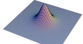
Figure 1: The curvature (2) mimics a regularized delta–function.

From the Kähler potential all geometrical quantities can be derived in the standard way, in particular, the curvature 2–form reads

$${\cal R}=\frac{r}{r+X}\!\begin{pmatrix}\displaystyle e\,{\bar{e}}-{\bar{e}}\,e+\frac{1}{n}\,\frac{{\bar{\epsilon}}\,\epsilon}{r+X}~{}\quad\frac{{\bar{\epsilon}}\,e}{\sqrt{r+X}}\\[12.91663pt] \displaystyle\frac{{\bar{e}}\,\epsilon}{\sqrt{r+X}}~{}\quad n\,{\bar{e}}\,e-\frac{n\!-\!1}{n}\,\frac{{\bar{\epsilon}}\,\epsilon}{r+X}\end{pmatrix}.$$ (2)

Here $e$ and $\epsilon$ are the holomorphic vielbein 1–forms of $\mathbb{CP}^{n-1}$ and its complex line bundle. An impression of the curvature is given in figure 1. This geometry admits a $\mathrm{U(1)}$ gauge background satisfying the Hermitian Yang–Mills equations

$$i{\cal F}_{V}=\Big{(}\frac{r}{r+X}\Big{)}^{1-\frac{1}{n}}\Big{(}{\bar{e}}e-\frac{n-1}{n^{2}}\,\frac{1}{r+X}\,{\bar{\epsilon}}\epsilon\Big{)}H_{V}~{},$$ (3)

where $H_{V}=V^{I}H_{I}$ with $H_{I}$ Cartan generator and $V^{I}$ either all integers or half integers. Because both the geometry and its $\mathrm{U(1)}$ gauge background are given explicitly, integrals of them can be computed:

$$\int_{\mathbb{CP}^{2}}\frac{\text{tr}\,{\cal R}^{2}}{(2\pi i)^{2}}=-n\,\int_{\mathbb{CP}^{1}\ltimes\mathbb{C}}\frac{\text{tr}\,{\cal R}^{2}}{(2\pi i)^{2}}=n(n+1)~{},$$ (4)

$$\int_{\mathbb{CP}^{p}}\Big{(}\frac{i{\cal F}}{2\pi i}\Big{)}^{p}~{}=~{}-n\int_{\mathbb{CP}^{p-1}\ltimes\mathbb{C}}\Big{(}\frac{i{\cal F}}{2\pi i}\Big{)}^{p}~{}=~{}1~{}.$$ (5)

The integrals over $\mathbb{CP}^{p}$ are taken at $X=0$ integrating over $p$ of the $n-1$ inhomogeneous coordinates of $\mathbb{CP}^{n-1}$. The integral over $\mathbb{CP}^{p-1}\ltimes\mathbb{C}$ corresponds to the integral over all values of $x\in\mathbb{C}$ and over $p-1$ inhomogeneous coordinates.

Using the explicit geometry of the blowup of $\mathbb{C}^{3}/\mathbb{Z}_{3}$ with $\mathrm{U(1)}$ gauge bundle, we can construct string compactifications. The integrated Bianchi identity integrated over $\mathbb{CP}^{2}$ has to vanish, giving: $V^{2}=12.$ The same condition is found when integrating over $\mathbb{CP}^{1}\ltimes\mathbb{C}$ and selects 7 allowed models listed in table 1. The spectra of these models can be compute using an index theorem. The multiplicities of the representations obtained from the branching of the adjoint of $\mathrm{SO(32)}$ via the multiplicity operator $N_{V}$ which can take the values: $N_{V}=\frac{1}{9},~{}1,~{}\frac{26}{9}=3-\frac{1}{9}$. The multiplicity factor $\frac{1}{9}=\frac{3}{27}$ refers to untwisted (delocalized) states, while integral multiplicity factors correspond to states localized at the orbifold fixed point Gmeiner:2002es . The table 1 compares the matter on the blowup with the heterotic orbifold spectrum in the blow down limit, and shows that only sometimes some vector–like matter is not recovered on the blowup.

Table 1: The first column displays the heterotic $\mathbb{Z}_{3}$ $\mathrm{SO(32)}$ orbifold shifts. The $\mathrm{U(1)}$ bundles on the blowup are defined by the second column. The gauge groups of the heterotic orbifold models are listed in the next column. The one but last column contains the matter representations on the resolution. The last column gives the additional twisted matter.

Orbifold	Blowup	$G_{\rm orbifold}=$	Matter spectrum on the	Additional
shift	shift	$G_{\rm blow\ down}$	orbifold resolution	twisted matter
$(0^{13},1^{2},2)$	$(0^{12},1^{3},3)$	$\mathrm{SO(26)}\times\mathrm{U(3)}$	$\frac{1}{9}(\mathbf{26},\mathbf{3})+\frac{26}{9}(\mathbf{1},\overline{\mathbf{3}})+(\mathbf{26},\mathbf{1})$	$(\mathbf{1},\mathbf{1})$
	$(0^{13},2^{3})$		$\frac{1}{9}(\mathbf{26},\overline{\mathbf{3}})+\frac{26}{9}(\mathbf{1},\mathbf{3})$	$(\mathbf{1},\mathbf{1})+(\mathbf{26},\mathbf{1})$
$(0^{10},1^{4},2^{2})$	$(0^{10},1^{4},2^{2})$	$\mathrm{SO(20)}\times\mathrm{U(6)}$	$\frac{10}{9}(\mathbf{1},\overline{\mathbf{15}})+\frac{1}{9}(\mathbf{20},\mathbf{6})+3(\mathbf{1},\mathbf{1})$
$(0^{7},1^{6},2^{3})$	$(0^{7},1^{8},2)$	$\mathrm{SO(14)}\times\mathrm{U(9)}$	$\frac{1}{9}(\mathbf{14},\mathbf{9})+\frac{1}{9}(\mathbf{1},\overline{\mathbf{36}})+(\mathbf{1},\overline{\mathbf{9}})$
$(0^{4},1^{8},2^{4})$	$(0^{4},1^{12})$	$\mathrm{SO(8)}\times\mathrm{U(12)}$	$\frac{1}{9}(\mathbf{8},\mathbf{12})+\frac{1}{9}(\mathbf{1},\overline{\mathbf{66}})$	$(\mathbf{1},\mathbf{1})+(\mathbf{8_{+}},\mathbf{1})$
	$(\frac{1}{2}^{12},\frac{3}{2}^{4})$		$\frac{1}{9}(\mathbf{8},\overline{\mathbf{12}})+\frac{1}{9}(\mathbf{1},\mathbf{66})+(\mathbf{8_{+}},\mathbf{1})$	$(\mathbf{1},\mathbf{1})$
$(0^{1},1^{10},2^{5})$	$\!(\frac{1}{2}^{14},\frac{3}{2},{\,\mbox{-}}\frac{5}{2})$	$\mathrm{SO(2)}\times\mathrm{U(15)}$	$\frac{11}{9}(\mathbf{15})+\frac{1}{9}(\overline{\mathbf{105}})+3(\mathbf{1})$

3 Toric resolutions of orbifold singularities

Figure 2: Projected views of the toric diagrams of the resolutions of $\mathbb{C}^{3}/\mathbb{Z}_{3}$ (left) and $\mathbb{C}^{3}/\mathbb{Z}_{4}$ (right).

We do not have the time to explain the properties of toric geometry Fulton ; Hori:2003ic ; Lust:2006zh in detail. The rough idea of toric resolutions of orbifold singularities is to replace the orbifold action by invariance $\mathbb{C}^{*}$ scalings of the coordinates $z_{i}$. To keep the dimensionality of the resolution equal to that of the orbifold one needs to introduce as many extra coordinates $x_{p}$ as complex scalings. Setting one of the homogeneous coordinates of the resolution defines a codimension one hypersurface called a divisor. Ordinary divisors are defined by $D_{i}=\{z_{i}=0\}$, and exceptional divisors by $E_{p}=\{x_{p}=0\}$. To each divisor we can associate a line bundle characterized by the transition functions between the various coordinate patches of the defining equation of the divisor. The first Chern class of a line bundle is a $(1,1)$–form, and hence we can reinterpret the divisors as $(1,1)$–forms themselves. Not all divisors are independent because of so–called linear equivalence relations among them

$$\sum_{i}(v_{i})_{j}\,D_{i}~{}+~{}\sum_{p}(w_{p})_{j}\,E_{p}~{}\sim~{}0~{}.$$ (6)

As there are as many such linear equivalence relations as ordinary divisors, we may take the exceptional divisors as a basis for the gauge background ${\cal F}_{V}$.

As hypersurfaces the divisors can intersect multiple times. These intersection numbers can be reinterpreted as integrals of the corresponding $(1,1)$–forms over the whole resolution. The intersections define the complete topology of the resolution. This topological information is conveniently summarized in the toric diagram: In a toric diagram the divisors are denoted as nodes, curves i.e. intersection of two divisors as lines between two nodes, and intersections of three different divisors as cones spanned by three nodes. Basic cones, the smallest possible cones, define intersections of three divisors with unit intersection number, while lines of three nodes correspond to intersection number zero. Together with the linear equivalence relations the toric diagram determines all (self–)intersections.

4 Toric resolution of $\boldsymbol{\mathbb{C}^{3}/\mathbb{Z}_{3}}$

We illustrate the power of toric geometry by reproducing the results obtained using the explicit blowup of $\mathbb{C}^{3}/\mathbb{Z}_{3}$. The toric resolution of this orbifold has three ordinary divisors $D_{i}$, and a single exception one $E$. They satisfy the linear equivalence relations:

$${D_{i}~{}\sim D_{j}}~{},\qquad{3\,D_{i}}\,+\,{E}~{}\sim~{}0~{},$$ (7)

From the toric diagram, left picture in figure 2, we infer the basic integrals and intersections: ${D_{1}D_{2}E}={D_{2}D_{3}E}={D_{3}D_{1}E}=1.$ The gauge field strength can be expanded as ${\cal F}_{V}=-\frac{1}{3}\,E\,H_{V}$. We obtained all the results of the explicit blowup. In particular, the Bianchi identity on the compact cycle $E$ gives:

$$V^{2}=\int_{E}\text{tr}(i{\cal F}_{V})^{2}=\int_{E}\text{tr}\,{\cal R}^{2}=12~{}.$$ (8)

The non–compact Bianchi identity follows immediately upon using the linear equivalence relation (7) and leads to the same condition.

5 Heterotic models on resolution of $\boldsymbol{\mathbb{C}^{3}/\mathbb{Z}_{4}}$

The main advantage of using toric geometry over explicit blowups lies in the fact that one can still use toric techniques in cases where no explicit blowup is known. To exemplify this we consider the resolution of $\mathbb{C}^{3}/\mathbb{Z}_{4}$. In this case there are two exceptional divisors $E_{1}$ and $E_{2}$, which satisfy the linear equivalence relations

$$4\,D_{1}\,+\,E_{1}\,+\,2\,E_{2}~{}\sim~{}0~{},\quad 4\,D_{2}\,+\,E_{1}\,+\,2\,E_{2}~{}\sim~{}0~{},$$

$$2\,D_{3}\,+\,E_{1}~{}\sim~{}0~{}.$$ (9)

To define the integrals on the resolution of $\mathbb{C}^{3}/\mathbb{Z}_{4}$ we use the toric diagram, on the right hand side of figure 2, and obtain

$${D_{1}\,E_{1}\,E_{2}}={D_{2}\,E_{1}\,E_{2}}={D_{1}\,D_{3}\,E_{1}}={D_{2}\,D_{3}\,E_{1}}=1~{},$$

$$D_{1}\,D_{2}\,E_{2}=D_{3}\,E_{1}\,E_{2}=0~{}.$$ (10)

Via the linear equivalences this implies:

$$E_{1}^{2}\,E_{2}=0~{},~{}E_{2}^{2}\,E_{1}=-2~{},~{}E_{1}^{3}=8~{},~{}E_{2}^{3}=2~{}.$$ (11)

The bottom edge of the toric diagram defines the toric diagram of the resolution of $\mathbb{C}^{2}/\mathbb{Z}_{2}$. The gauge background is expanded in terms of the exceptional divisors

$${{{\cal F}_{V}}=-\frac{1}{2}\,E_{1}\,H_{1}\,-\,\frac{1}{4}\,(E_{1}+2\,E_{2})H_{2}~{},}$$ (12)

where $H_{1}=V_{1}^{I}H_{I}$, etc. In order to ensure that we can directly compute the spectrum on the non–compact resolution, we require that all the Bianchi identities vanish on $E_{1}$, $E_{2}$ and the resolution of $\mathbb{C}^{2}/\mathbb{Z}_{2}$:

$$E_{1}:~{}~{}{V_{1}^{2}\,+\,V_{1}\cdot V_{2}~{}=~{}4}~{},\quad E_{2}:~{}~{}{V_{1}\cdot V_{2}~{}=~{}-2~{},}$$

$$\text{Res}(\mathbb{C}^{2}/\mathbb{Z}_{2}):~{}~{}{V_{2}^{2}~{}=~{}6~{}.}$$ (13)

The matching between the heterotic orbifold models and the resolution models characterized by the shifts $V_{1}$ and $V_{2}$ is performed in table 2. All models except number 4 is reproduced in blowup. This model is not obtained because it does not have any first twisted sector, hence simply cannot be blown up. We have computed the complete spectrum and confirmed that all blowup models have anomaly free spectra Nibbelink:2007pn .

Table 2: This table compares the $\mathbb{C}^{3}/\mathbb{Z}_{4}$ orbifold gauge shift vector $v\,$, with the blowup vectors $V_{1}$ and $V_{2}\,$, that characterize the line bundle gauge background on the resolution.

orbifold blowup blowup shift $4\,v$ vector $V_{2}$ vector $V_{1}$ Nr. $(0^{13},1^{2},2)$ $(0^{13},1^{2},2)$ $(0^{13},1^{2},$-$2)$ 1a $(0^{13},1^{2},2)$ $(0^{12},2,$-$1^{2},0)$ 1b $(0^{13},1^{2},2)$ $(0^{11},2,1,0^{2},$-$1)$ 1c $(0^{11},1^{2},2^{3})$ $(0^{13},1^{2},2)$ $(0^{10},1^{4},$-$1^{2})$ 2a $(0^{13},1^{2},2)$ $(0^{11},1^{2},$-$2,0^{2})$ 2b $(0^{9},1^{2},2^{5})$ $(0^{13},1^{2},2)$ $(0^{8},1^{5},0^{2},$-$1)$ 3a $(0^{13},1^{2},2)$ $(0^{9},1^{4},$-$1^{2},0)$ 3b $(0^{7},1^{2},2^{7})$ $-$ $-$ 4 $(0^{10},1^{6})$ $(0^{10},1^{6})$ $(0^{10},1^{2},$-$1^{4})$ 5a $(0^{10},1^{6})$ $(0^{13},1,$-$1,$-$2)$ 5b $(0^{10},1^{5},3)$ $(0^{10},1^{6})$ $(0^{9},2,$-$1^{2},0^{4})$ 6 $(0^{8},1^{6},2^{2})$ $(0^{10},1^{6})$ $(0^{8},1^{3},$-$1^{3},0^{2})$ 7a $(0^{10},1^{6})$ $(0^{8},1^{2},$-$2,0^{5})$ 7b $(0^{6},1^{6},2^{4})$ $(0^{10},1^{6})$ $(0^{6},1^{4},$-$1^{2},0^{4})$ 8

orbifold blowup blowup shift $4\,v$ vector $V_{2}$ vector $V_{1}$ Nr. $(0^{5},1^{10},2)$ $(0^{10},1^{6})$ $\frac{1}{2}($-$3,1^{10},$-$1^{5})$ 9 $(0^{3},1^{10},2^{3})$ $(0^{10},1^{6})$ $\frac{1}{2}(1^{12},$-$1^{3},$-$3)$ 10 $(1^{14},2^{2})$ $(0^{13},$-$2,1^{2})$ $\frac{1}{2}(1^{15},$-$3)$ 11 $(1^{13},$-$1,2^{2})$ $(0^{13},1^{2},2)$ $\frac{1}{2}(1^{15},$-$3)$ 12a $(0^{13},1^{2},2)$ -$\frac{1}{2}($-$3,1^{15})$ 12b $\frac{1}{2}(1^{3},3^{12},$-$3)$ $\frac{1}{2}($-$3,1^{15})$ -$(0^{13},1^{2},2)$ 13a $\frac{1}{2}(1^{15},$-$3)$ $(0^{13},1^{2},2)$ 13b $\frac{1}{2}(1^{15},$-$3)$ $\frac{1}{2}(1^{3},$-$1^{11},3,1)$ 13c $\frac{1}{2}(1^{7},3^{8},$-$3)$ $\frac{1}{2}(1^{15},$-$3)$ $($-$1^{5},1,0^{10})$ 14a $\frac{1}{2}(1^{15},$-$3)$ $\frac{1}{2}(1^{6},$-$1^{8},$-$3,1)$ 14b $\frac{1}{2}(1^{11},3^{4},$-$3)$ $\frac{1}{2}(1^{15},$-$3)$ $(0^{10},1^{3},$-$1^{3})$ 15 $\frac{1}{2}(1^{15},$-$3)$ $\frac{1}{2}(1^{15},$-$3)$ $(0^{13},$-$2,1^{2})$ 16a $\frac{1}{2}(1^{15},$-$3)$ $\frac{1}{2}($-$1^{14},3,$-$1)$ 16b

References

• (1) A. E. Faraggi, D. V. Nanopoulos, and K.-j. Yuan Nucl. Phys. B335 (1990) 347.
• (2) A. E. Faraggi Phys. Lett. B278 (1992) 131–139.
• (3) M. Berkooz, M. R. Douglas, and R. G. Leigh Nucl. Phys. B480 (1996) 265–278 [hep-th/9606139].
• (4) R. Blumenhagen, L. Goerlich, B. Kors, and D. Lust JHEP 10 (2000) 006 [hep-th/0007024].
• (5) G. Aldazabal, S. Franco, L. E. Ibanez, R. Rabadan, and A. M. Uranga J. Math. Phys. 42 (2001) 3103–3126 [hep-th/0011073].
• (6) G. Honecker and T. Ott Phys. Rev. D70 (2004) 126010 [hep-th/0404055].
• (7) T. P. T. Dijkstra, L. R. Huiszoon, and A. N. Schellekens Nucl. Phys. B710 (2005) 3–57 [hep-th/0411129].
• (8) T. P. T. Dijkstra, L. R. Huiszoon, and A. N. Schellekens Phys. Lett. B609 (2005) 408–417 [hep-th/0403196].
• (9) P. Candelas, G. T. Horowitz, A. Strominger, and E. Witten Nucl. Phys. B258 (1985) 46–74.
• (10) B. Andreas, G. Curio, and A. Klemm Int. J. Mod. Phys. A19 (2004) 1987 [hep-th/9903052].
• (11) V. Braun, Y.-H. He, B. A. Ovrut, and T. Pantev JHEP 06 (2005) 039 [hep-th/0502155].
• (12) R. Blumenhagen, G. Honecker, and T. Weigand JHEP 10 (2005) 086 [hep-th/0510049].
• (13) R. Blumenhagen, S. Moster, and T. Weigand Nucl. Phys. B751 (2006) 186–221 [hep-th/0603015].
• (14) L. Dixon, J. A. Harvey, C. Vafa, and E. Witten Nucl. Phys. B261 (1985) 678–686.
• (15) L. J. Dixon, J. A. Harvey, C. Vafa, and E. Witten Nucl. Phys. B274 (1986) 285–314.
• (16) S. Forste, H. P. Nilles, P. K. S. Vaudrevange, and A. Wingerter Phys. Rev. D70 (2004) 106008 [hep-th/0406208].
• (17) T. Kobayashi, S. Raby, and R.-J. Zhang Nucl. Phys. B704 (2005) 3–55 [hep-ph/0409098].
• (18) T. Kobayashi, S. Raby, and R.-J. Zhang Phys. Lett. B593 (2004) 262–270 [hep-ph/0403065].
• (19) W. Buchmuller, K. Hamaguchi, O. Lebedev, and M. Ratz Nucl. Phys. B712 (2005) 139–156 [hep-ph/0412318].
• (20) O. Lebedev et al. Phys. Lett. B645 (2007) 88–94 [hep-th/0611095].
• (21) J. E. Kim and B. Kyae Nucl. Phys. B770 (2007) 47–82 [hep-th/0608086].
• (22) T. Eguchi and A. J. Hanson Phys. Lett. B74 (1978) 249.
• (23) E. Calabi Ann. Scient. ´Ecole Norm. Sup. 12 (1979) 269.
• (24) J. Erler and A. Klemm Commun. Math. Phys. 153 (1993) 579–604 [hep-th/9207111].
• (25) O. J. Ganor and J. Sonnenschein JHEP 05 (2002) 018 [hep-th/0202206].
• (26) S. Groot Nibbelink, M. Trapletti, and M. Walter JHEP 03 (2007) 035 [hep-th/0701227].
• (27) R. Blumenhagen, G. Honecker, and T. Weigand JHEP 08 (2005) 009 [hep-th/0507041].
• (28) S. Groot Nibbelink, H. P. Nilles, and M. Trapletti [hep-th/0703211].
• (29) S. Groot Nibbelink, T.-W. Ha, and M. Trapletti [arXiv:0707.1597 [hep-th]].
• (30) G. Honecker and M. Trapletti JHEP 01 (2007) 051 [hep-th/0612030].
• (31) F. Gmeiner, S. Groot Nibbelink, H. P. Nilles, M. Olechowski, and M. Walter Nucl. Phys. B648 (2003) 35–68 [hep-th/0208146].
• (32) W. Fulton Introduction to Toric Varieties. Princeton University Press 1993.
• (33) K. Hori et al. Mirror symmetry. Providence, USA: AMS (2003) 929 p.
• (34) D. Lust, S. Reffert, E. Scheidegger, and S. Stieberger [hep-th/0609014].