Spectral methods and cluster structure in correlation-based networks

Abstract

We investigate how in complex systems the eigenpairs of the matrices derived from the correlations of multichannel observations reflect the cluster structure of the underlying networks. For this we use daily return data from the NYSE and focus specifically on the spectral properties of weight $W_{ij}=|C|_{ij}-\delta_{ij}$ and diffusion matrices $D_{ij}=W_{ij}/s_{j}-\delta_{ij}$, where $C_{ij}$ is the correlation matrix and $s_{i}=\sum_{j}W_{ij}$ the strength of node $j$. The eigenvalues (and corresponding eigenvectors) of the weight matrix are ranked in descending order. In accord with the earlier observations the first eigenvector stands for a measure of the market correlations. Its components are to first approximation equal to the strengths of the nodes and there is a second order, roughly linear, correction. The high ranking eigenvectors, excluding the highest ranking one, are usually assigned to market sectors and industrial branches. Our study shows that both for weight and diffusion matrices the eigenpair analysis is not capable of easily deducing the cluster structure of the network without a priori knowledge. In addition we have studied the clustering of stocks using the asset graph approach with and without spectrum based noise filtering. It turns out that asset graphs are quite insensitive to noise and there is no sharp percolation transition as a function of the ratio of bonds included, thus no natural threshold value for that ratio seems to exist. We suggest that these observations can be of use for other correlation based networks as well.

, , , , and

1 Introduction

The network approach to complex systems has turned out to be extremely fruitful in revealing their structure and function [1, 2, 3, 4]. The usual way to construct the network is to identify the elements of the system with nodes, between which the links are present if the corresponding interactions exist. In the case of weighted networks, the weight of a link is identified with the strength of the interaction.

Processes taking place in a complex system, represented as a network, depend heavily on its structure. For example motifs that are statistically significantly overrepresented as compared to a random reference system are supposed to have some functional role [5, 6]. Moreover, communities i.e. groups that are well wired internally but loosely connected to the rest of the network, play an eminent role in dynamic phenomena like spreading [7, 8, 9]. Clearly, the investigation of the network structure is of central interest.

For many systems, however, the nature of interactions is hidden and only some activities of the nodes can be measured, e.g., in the form of time series. For such systems, the natural network representation is a complete graph with weights corresponding to the elements of the correlation matrix determined by the nodal activities. Then the task is to filter out from the noisy correlation matrix the groups of closely related elements. This problem is quite general and it appears in many fields of research ranging from the evaluation of micro-array data to portfolio optimization. In this paper we have chosen to study correlation matrices of stock returns, but we think that the network approach and the observations made here have also more general validity.

Correlations between time-series of stock returns serve as one of the main inputs in the portfolio optimization theory. In the classical Markowitz portfolio optimization the correlations are used as measures of the dependence between the time series and the variance as the measure of risk [10]. As the empirical time series are always finite, the resulting correlation matrix is noisy. This brings up the need to reduce the noise, for which the most frequently applied tool in the financial literature is principal component analysis [12].

Previously, correlation matrices of stock return time series have been studied from the network point of view, e.g., by using maximal spanning trees (MST). The maximal spanning tree of a network is a tree containing all the $N$ nodes and $N-1$ links such that the sum of the weights is maximized. It was introduced in the study of financial correlation matrices by Mantegna [13], who was able to identify groups of stocks that make sense from an economic point of view. It was discovered that often, the branches of the MST correspond to business sectors or industries. Moreover, this method enables to describe the hierarchical organization of the market and has been applied to monitor the effect of the time dependence of the correlations [17] Later, MSTs of diverse financial correlation based networks have been studied, e.g., by Bonanno et al. [14, 15, 16] and Onnela et al. [17, 18]. Indeed, the MST method is simple and gives reasonable results. However, it is too restrictive and thus other, complementary methods are needed.

In the so called asset graph approach, one ranks the links according to the values of the corresponding correlation matrix and considers only a fraction $p$ of the strongest ones as occupied. By using this method for low values of $p$ Onnela et al. [19] and Heimo et al. [20] found clear evidence of strong intra-business sector clustering. It has also been suggested that planar maximally filtered graphs yield a natural extension to the MST approach [21]. Other interesting approaches include methods based on the super-paramagnetic Potts model [22] and on the maximum likelihood optimization [23]. Several financial markets have been studied from the above points of view.

Based on these approaches a following picture about the organization of the correlation network of the stocks emerges: i) There is a dominant correlation among most of the stocks reflecting the overall behavior of the market (this is the basis of the one factor model [11]); ii) The stocks are organized hierarchically in clusters, which mainly correspond to industrial branches (as assumed in the multi-factor models) [11] iii) There are systematic deviations from this oversimplified picture, partly because of the ambiguous nature of any classification scheme and partly because of inter-cluster relations; iv) In spite of considerable robustness in the correlations during the time of "business as usual", major events like crashes cause dramatic changes in the network structure [17].

All information on the network structure is encoded in its adjacency matrix, or, for weighted networks, in the weight matrix. Likewise, all information on the structure of correlations of stock returns is to be found in the correlation matrix. Consequently, this information is also inherited by the eigenvalues and eigenvectors of such matrices. If the data is structured in terms of clusters and communities that these matrices represent, it should also be reflected in the eigenpairs. For financial correlation matrices, it has been shown that most eigenpairs correspond to noise accessible by random matrix theory and thus the information about the cluster structure is contained in a few non-random eigenpairs [24, 25, 26] (see [27] for an overview). It was also suggested that clusters of highly correlated stocks could be identified by studying the localization of non-random eigenvectors. In this paper we investigate the questions of how the eigenpairs of correlation and related matrices derived from stock price time series reflect the cluster structure and industry sectors.

This paper is organized as follows. Section 2 gives a short introduction to the spectral properties of weight and diffusion matrices and their relationship to the cluster structure of the underlying network. Section 3 is devoted to the analysis of the largest eigenvalue and the corresponding eigenvector, whereas the intermediate, non-random eigenpairs are examined in Section 4. The asset graph approach to the clustering of stocks is discussed in Section 5.

2 Basic notions

2.1 Matrices related to weighted networks

A simple undirected and weighted network can be represented by a weight matrix $\boldsymbol{W}$ in which an element $W_{ij}=W_{ji}$ ($\geq 0$ in our study) corresponds to the weight of the link between the nodes $i$ and $j$ and the diagonal elements are zero. Note that $W_{ij}=0$ signifies the absence of the link. The sum $s_{i}=\sum_{j}W_{ij}$ is the strength of node $i$ [28]. Here, we restrict our analysis to irreducible networks, i.e., networks consisting of just one connected component. In this case the Frobenius-Perron theorem states that $\boldsymbol{W}$ has a largest positive eigenvalue and the components of the corresponding eigenvector are non-zero and of the same sign.

If the elements of $\boldsymbol{W}$ are i.i.d. random numbers with finite variance $\sigma^{2}$, the probability density of the first eigenvalue converges to a normal distribution [30]

$$\lim_{N\to\infty}\operatorname{distr}\left\{\lambda_{1}-\left[(N-1)\mu+\sigma^{2}/\mu\right]\right\}=\mathcal{N}(0,2\sigma^{2})$$ (1)

where $\mu>0$ is the mean of the matrix elements. The first term inside the square brackets expresses the average node strength, while the second term is due to fluctuations. In some cases statements can be made about the whole spectrum. We return to this in section 2.3.

Diffusion process in terms of random walks can be used as a tool for studying the structure of a network [31, 32, 33]. At each time step a walker moves at random from its current node $j$ to node $i$ with probability $T_{ij}=W_{ij}/s_{j}$. If we denote the walker density at node $i$ by $v_{i}(t)$, the average dynamics of the process is described by

$$\vec{v}(t+1)=\boldsymbol{T}\vec{v}(t)$$ (2)

or equivalently by

$$\vec{v}(t+1)-\vec{v}(t)=\boldsymbol{D}\vec{v}(t),$$ (3)

where $\vec{v}(t)=(v_{1}(t),\ldots,v_{N}(t))^{T}$ and $\boldsymbol{D}=\boldsymbol{T}-\boldsymbol{I}$. Here, $\boldsymbol{T}$ denotes the transfer matrix and $\boldsymbol{D}$ the diffusion matrix. These matrices have clearly the same eigenvectors and the spectrum of $\boldsymbol{D}$ is identical with the spectrum of $\boldsymbol{T}$ shifted to the left by unity. The matrix $\boldsymbol{T}$ can be mapped into a symmetric matrix by the similarity transformation $\operatorname{diag}(s_{i}^{-1/2})\cdot\boldsymbol{T}\cdot\operatorname{diag}(s_{i}^{1/2})$ and therefore its eigenvalues are real. Futhermore, the walker density cannot diverge at any node, so the eigenvalues of $\boldsymbol{T}$ must lie within the interval $[-1,1]$. The strength vector $\vec{s}=(s_{1},\ldots,s_{N})$ is an eigenvector of $\boldsymbol{T}$ with eigenvalue $1$ and due to the Frobenius-Perron theorem this eigenvalue is non-degenerate. Thus

$$\lim_{t\to\infty}\vec{v}(t)=\vec{s},$$ (4)

unless the network is bipartite, in which case $-1$ is also an eigenvalue.

In addition to walker densities $v_{i}(t)$, the diffusion process can also be analyzed by studying the walker densities per unit strength defined by

$$c_{i}(t)=\frac{v_{i}(t)}{s_{i}}.$$ (5)

It is straightforward to show that

$$\vec{c}(t+1)=\boldsymbol{N}\vec{c}(t),$$ (6)

where $\boldsymbol{N}=\boldsymbol{T}^{T}$ is called the normal matrix. Clearly the only difference between the governing equations for the densities and the densities per unit strength is that $\boldsymbol{T}$ is replaced with $\boldsymbol{N}$. From Eq. (4) we see that

$$\lim_{t\to\infty}\vec{c}(t)=(1,\ldots,1)^{T}.$$ (7)

2.2 Modular structure and eigenvectors

Recently there has been increasing interest in the "mesoscopic" properties of networks, i.e., in structures beyond the scale of single vertices or their immediate neighborhoods. One important related problem is the detection and characterization of modules or communities [7, 8, 34, 35, 36, 37], which are, loosely speaking, groups of vertices with dense internal connections and weaker connections to the rest of the network.

Evidently, the weight, transfer, normal, and diffusion matrix representations of a modular network carry information about the modules in their eigenvalues and -vectors. In the case of diffusion, it is tempting to assign to the eigenvalues and -vectors a direct physical interpretation [31, 32, 33]. If a random walker enters a module with dense internal connections and sparse connections to the rest of the network, it gets, on average, “trapped” for a long time. This phenomenon is reflected to the spectral expansion of the random walker density at time $t$,

$$v_{i}(t)=\sum_{j}c_{j}\lambda_{j}^{t}\cdot[\vec{e}_{j}]_{i}$$ (8)

$$\vec{c}=\boldsymbol{E}^{-1}\vec{v}(0),$$ (9)

where $\boldsymbol{E}$ contains the eigenvectors $\vec{e}_{j}$ of the transfer matrix in its columns. If convergence to the stationary state is slow, Eq. (8) should contain some terms with eigenvalues close to $1$ or $-1$. Eigenvalues close to $-1$ indicate that the network is almost bipartite. On the other hand, large positive eigenvalues are consequences of modular structure and the corresponding eigenvectors can be expected to carry information about the structure of communities.

The interpretation of the eigenpairs of the weight matrix is more difficult. However, one can naturally iterate a vector $\vec{v}$ (a ”phantom field” on the nodes of the network) by the weight matrix, and study its properties. Eq. (8) still applies, and Eq. (9) can be written in a simpler form $c_{j}=\vec{e}_{j}\cdot\vec{v}(0)$ due to the symmetry of the weight matrix (of course, $\vec{e}_{j}$ are now eigenvectors of the weight matrix). Here a convenient initial condition is $v_{j}(0)=\delta_{ij}$, and as $v_{a}(t+1)=\sum_{j}W_{aj}v_{j}(t)$, the new value of this quantity on node $a$ will be a weighted sum of the (old) values on $a$’s neighbours. If the spreading of this quantity starts from node $i$, located in a densely interconnected module, during the first time steps only the other members of this module get significant contribution, as $i$ and its neighbours have most of their links within the module. The phenomenon resembles the “trap”-behaviour of the modules in the case of diffusion. Noticing that

$$\frac{\vec{v}(t)}{\lambda_{1}^{t}}=\frac{\boldsymbol{W}^{t}\vec{v}(0)}{\lambda_{1}^{t}}\xrightarrow[t\to\infty]{}\vec{e}_{1},$$ (10)

where $\lambda_{1}$ is the largest eigenvalue of $\boldsymbol{W}$, we see that the ratios $v_{i}/v_{j}$ approach to constants. The speed of the convergence depends naturally on the magnitudes of the other eigenvalues.

The fact that eigenvalues close to the largest one slow down the convergence, suggests that the corresponding eigenvectors can carry information about the modules, similarly to the eigenvectors of the diffusion matrix. In conclusion, it seems to be reasonable to interpret the eigenvectors of the weight matrix similarly to the eigenvectors of the diffusion matrix, at least from the point of view of network modularity.

Now, let us turn shortly to the interpretation of eigenvector components, both for diffusion and weight matrices. Consider a case in which the eigenvectors are ranked in descending order and $\lambda_{2}\gg|\lambda_{3\ldots N}|\approx 0$. Assume that the second eigenvector is localized on two sets of nodes, such that the eigenvector components corresponding to the first set are positive, and the components corresponding to the second set are negative. Then, the second term in Eq. (8) gives a slowly decaying correction for both sets of nodes, but with different signs. This means that the random walker or the “phantom field” gets trapped for a while in one set, and is held back from entering into the other set. So the first set of nodes can be thought of as a community. Changing the initial condition such that $c_{2}$ changes its sign, and applying the above arguments shows that the other set can also be thought of as a community. Both of these cases show that the two communities are far from each other as regards to the average travelling time of a random walker between them. It should be noted here that using absolute values or squares of the eigenvector components (e.g. [38], [39]) is clearly inappropriate, as an eigenvector may be localized on two extremely distant communities.

As mentioned in the previous section the diffusion process can also be analyzed by studying the time evolution of the walker densities per unit strength $c_{i}(t)$. Simonsen et al. have suggested that the eigenvectors of the normal matrix $\boldsymbol{N}$ corresponding to the largest eigenvalues contain a lot of information about the modular structure of the network and that the modules can be identified with the so called current mapping technique [31, 32, 33]. Here, one should notice that the $i$th component of the $k$th eigenvector of $\boldsymbol{N}$ is equal to $[\vec{e}_{k}]_{i}/s_{i}$, where $[\vec{e}_{k}]_{i}$ is the $i$th component of the $k$th eigenvector of the transfer matrix $\boldsymbol{T}$.

2.3 Correlation Matrices

The equal time correlation matrix $\boldsymbol{C}$ of $N$ variables can be estimated from $T$ observations by

$$C_{ij}=\frac{\langle\mathbf{r}_{i}\mathbf{r}_{j}\rangle-\langle\mathbf{r}_{i}\rangle\langle\mathbf{r}_{j}\rangle}{\sqrt{[\langle{\mathbf{r}_{i}}^{2}\rangle-\langle\mathbf{r}_{i}\rangle^{2}][\langle{\mathbf{r}_{j}}^{2}\rangle-\langle\mathbf{r}_{j}\rangle^{2}]}},$$ (11)

where $\mathbf{r_{i}}$ is a vector containing the observations of the variable $i$. In the case of Gaussian i.i.d. variables, $\boldsymbol{C}$ is the Wishart matrix and its eigenvalue density converges as $N\to\infty$, $T\to\infty$, while $N/T\leq 1$ is fixed, to [40]

$$\rho_{\boldsymbol{W}}(\lambda)=\left\{\begin{array}[]{ll}\frac{T/N}{2\pi\sigma^{2}}\frac{\sqrt{(\lambda_{\textrm{max}}-\lambda)(\lambda-\lambda_{\textrm{min}})}}{\lambda}&\textrm{if }\lambda_{\textrm{min}}\leq\lambda\leq\lambda_{\textrm{max}}\\ 0&\textrm{else}\end{array}\right.$$ (12)

$$\lambda_{\textrm{max/min}}=\sigma^{2}\left(1\pm\sqrt{N/T}\right)^{2},$$ (13)

where $\sigma^{2}=1$ due to the “normalization” in Eq. (11). In empirical cases, significant deviations from Eq. (12) can usually be considered as signs of relevant information [26].

A correlation matrix can be transformed to weight matrix of a simple undirected and weighted network by

$$W_{ij}=|C_{ij}|-\delta_{ij}.$$ (14)

From the point of view of network theory, the transformation can be justified by interpreting the absolute values as measures of interaction strength without considering whether the interaction is positive or negative. If the elements of $\boldsymbol{C}$ are non-negative, $\boldsymbol{W}=\boldsymbol{C}-\boldsymbol{I}$. Therefore, the transformation does not change the eigenvectors but the eigenvalues are shifted to the left by unity. The correlation matrices studied in this paper, however, contain a few slightly non-negative elements. Fortunately, taking the absolute value of the elements does not change the numerical values of the spectral quantities significantly.

In the following sections, we study correlation matrices constructed from the logarithmic returns of New York Stock Exchange (NYSE) traded stocks. We use two different data sets. The larger one consists of the daily closing prices of 476 stocks and ranges from 2-Jan-1980 to 31-Dec-1999. In the smaller data set the number of stocks is 116 and the time window ranges from 13-Jan-1997 to 29-Jan-2000. With both data sets the length of the time series $T$ is not very large compared to the number of stocks $N$. Therefore the correlation matrices are noisy.

3 First eigenpair

The largest eigenvalue of a correlation matrix derived from stock return time series is always clearly separated from the rest of the spectrum. The corresponding eigenvector is typically interpreted to be representative of the whole market [26], and is usually called the market eigenvector.

3.1 Approximations of the first eigenvector

Perhaps the simplest way to approximate the first eigenvector of the weight matrix is to iterate a vector that is not perpendicular to the first eigenvector by the weight matrix (see Eq. (10)). From the Frobenius-Perron theorem we know that the components of the first eigenvector have the same sign, so a natural choice for the initial vector is one with uniform components. The first iteration of this vector yields a vector proportional to the strength vector $\vec{s}$. Since $\vec{s}$ is the first eigenvector of the diffusion matrix derived from the weight matrix, we see that the first eigenvectors of the weight and the diffusion matrices are the sime after first iteration. Of course, one can find examples where this approximation is far from the asymptotics.

Another simple way to approximate the first eigenvector of the weight matrix is a perturbation-based calculation. In [39], such an approach was presented, although with a different definition of perturbation. Here we separate the empirical weight matrix into two terms as

$$W_{ij}=(1-\delta_{ij})w_{0}+V_{ij},$$ (15)

where $w_{0}$ is the average off-diagonal element of the weight matrix and $V_{ij}$ is the deviation considered as perturbation. The eigenvalues of the unperturbed matrix are

$$\lambda_{1}^{(0)}=(N-1)w_{0},$$ (16)

$$\lambda_{2\ldots N}^{(0)}=-w_{0},$$ (17)

and the first eigenvector is

$$\vec{e}_{1}^{(0)}=\frac{1}{\sqrt{N}}(1,1,\ldots,1)^{T}$$ (18)

The first order correction of the first eigenvalue reads

$$\lambda_{1}^{(1)}=\vec{e}_{1}^{(0)^{T}}\boldsymbol{V}\vec{e}_{1}^{(0)}=\frac{1}{N}\sum_{ij}{V_{ij}}=0,$$ (19)

and thus $\lambda_{1}\approx(N-1)w_{0}$, assuming that the perturbation expansion converges fast. The first order correction of the first eigenvector is

$$\vec{e}_{1}^{(1)}=\frac{\boldsymbol{V}}{Nw_{0}}\cdot\vec{e}_{1}^{(0)}-\frac{\vec{e}_{1}^{(0)^{T}}\boldsymbol{V}\vec{e}_{1}^{(0)}}{Nw_{0}}\cdot\vec{e}_{1}^{(0)}=\frac{\boldsymbol{V}}{Nw_{0}}\cdot\vec{e}_{1}^{(0)},$$ (20)

and the $i$th component the corresponding first order approximation is

$$\left[\vec{e}_{1}^{(0)}+\vec{e}_{1}^{(1)}\right]_{i}=\frac{1}{\sqrt{N}}(1+\frac{s_{i}-\overline{s}}{Nw_{0}})\approx\frac{s_{i}}{\overline{s}\sqrt{N}},$$ (21)

where $N\gg 1$ has been assumed.

Thus the result is similar to the one obtained by the iterative way – in first order perturbation theory, the components of the first eigenvector are proportional to the corresponding strengths. This proportionality was also pointed out in Ref. [39]. We add to this observation that, provided the first order approximation is sufficient, the average off-diagonal matrix element is proportional to the largest eigenvalue.

3.2 First eigenpair of financial correlation based networks

Based on the previous section, it is not surprising that the largest eigenvalue $\lambda_{1}$ is strongly correlated with the mean correlation coefficient in both data sets used. This is illustrated in Fig. 1. Deviations from the zeroth order approximation are illustrated in Fig. 2.

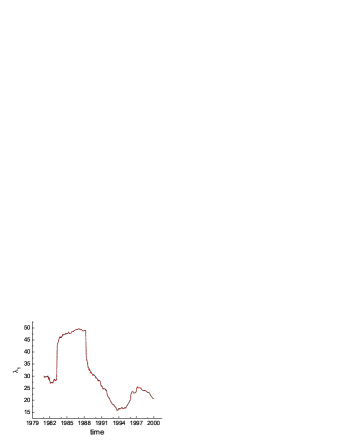
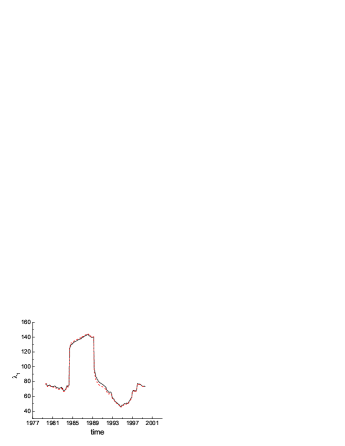
Figure 1: (color online) The first eigenvalues (solid line) and rescaled mean correlations (dashed line) as functions of time for the $116$-stocks database (on the left) and for the $476$-stocks database (on the right). The correlation matrices were constructed from 1000 trading days in both cases. The outstanding plateau is a consequence of Black Monday, a large market crash on October 19, 1987.

Figure 2: Difference between the first eigenvalue and its zeroth order approximation for the $116$-stocks dataset (on the left) and for the $476$-stocks dataset (on the right). A window of 1000 trading days has been used.

As expected, the eigenvector corresponding to the largest eigenvalue is well approximated by the strength vector. This is illustrated in Fig. 3.

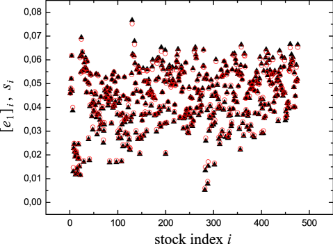
Figure 3: (color online) Components of the first eigenvector ($\blacktriangle$) and the normalized strengths ($\circ$) (the larger data set is used). The ordering of the stocks is such that stocks belonging to same business sector according to Yahoo classification [41] are next to each other.

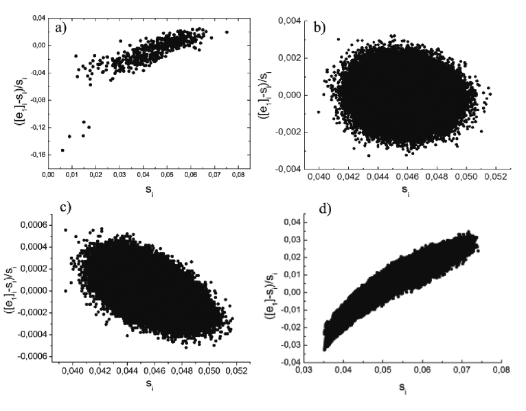
Figure 4: The relative differences of the components of the first eigenvector and the (normalized) strength-vector as functions of the (normalized) strengths. a) The empirical data set ($N=476$ stocks), b) random matrices with $i.i.d$ elements from the uniform distribution, c) correlation matrices of the one factor model with the same length of time series and the same mean correlation as the empirical matrix, d) artificial multiblock correlation matrices. All results for artificial matrices are averages over 1000 runs.

A further observation is that the relative differences of the components of the first eigenvector and the (normalized) strengths are positively correlated with the strengths (Fig. 4, panel a). In order to understand this effect, we have constructed and numerically analyzed several kinds of correlation matrices. Our observations are as follows: the above correlation does not exist for random matrices, in which the elements are i.i.d. random variables from uniform distribution (Fig. 4, panel b). Surprisingly, the correlation is negative for the one factor model with the same mean correlation, when the correlation matrix is constructed from finite time segments of uncorrelated Gaussian time series [42] (Fig. 4, panel c). A strength distribution with non-vanishing width produces similar effect. However, for multi-block weight matrices with an artificial modular structure together with additional noise, similar correlation is found (Fig. 4, panel d). Hence, the observed correlation could be attributed to the presence of modular structure in the weight matrix.

There is another interesting feature in Fig. 4 worth noting. The "outliers" in the lower left corner of panel a in Fig. 4 correspond to companies related to gold and silver mining, which are known to be extremely weakly correlated (or even negatively correlated) with the other participants of the market.

4 Intermediate eigenpairs

In this section we analyze the intermediate eigenvectors of the empirical weight and diffusion matrices. We start by discussing the problems related to defining the information carrying eigenvectors of the weight matrix and continue by studying how the cluster structure of the network is reflected in the localization of these eigenvectors. Lastly, we analyze the intermediate eigenvectors of the diffusion matrix and find the highest ranking ones to be very close to those of the weigth matrix. We also demonstrate the use of the current mapping technique with our data set.

4.1 Defining the intermediate eigenpairs of the weight matrix

The highest ranking eigenpairs of the correlation matrix constructed from stock return time series are far from being random [24, 25], but the randomness increases rapidly together with increasing rank (on average) [20]. Therefore, there is no strict border between the random and intermediate parts of the spectrum and the identification of the information carrying eigenvectors is a highly non-trivial task.

Fig. 5 depicts the spectrum of the weight matrix together with the analytical results for Wishart matrices (Eq. (12)). The analytical curve is fitted by visual inspection using $\sigma$, i.e. the variance of the effectively random part of the correlation matrix, as an adjustable parameter. Best fit is obtained with $\sigma\approx 0.86$, which, substituted into Eq. (13), yields $\lambda_{max}\approx 0.3$. However, many eigenvectors corresponding to eigenvalues above this bound are to a large extent random and on the other hand, some below this bound contain information [43]. Therefore, $\lambda_{max}$ can only be considered as a suggestive indicator of the crossover region between the random and intermediate parts of the spectrum.

Figure 5: Left: The spectral density of the weight matrix. The inset shows the random bulk and the analytical curve. Right: The IPRs of the eigenvectors as a function of the corresponding eigenvalue.

Plerou et al. [25, 26] have suggested the use of inverse participation ratios (IPR), defined for vector $\vec{v}$ as

$$I(\vec{v})=\sum_{i}v_{i}^{\phantom{i}4},$$ (22)

in the identification of the information carrying eigenvectors. The idea behind this is that the more localized the eigenvector is, the higher is its IPR. From the right panel of Fig. 5, which depicts $I(\vec{v})$ for the eigenvectors of the weight matrix as a function of the corresponding eigenvalue, we see that most of the random and intermediate eigenvectors have similar IPRs (see also [43]). Thus IPR does not seem to be an efficient tool to distinguish the information carrying eigenvectors from the rest. More sophisticated analysis is needed.

4.2 Localization of the eigenvectors

We have seen that the gradual increase of the noise content aleady makes the identification of the clusters in the network a difficult task. Here we will go into the further difficulties caused be the complexity of the localization of the information carrying eigenvectors. Financial correlations are particularly appropriate to investigate this point as independent classification schemes exist to compare with. In the following we will take advantage of this information in the example-like analysis of a couple of interesting eigenvectors. The components of the eigenvectors studied are illustrated in Fig. 6, in which the (horizontal) ordering of the stocks is such that stocks belonging to same business sector according to Yahoo classification [41] are next to each other. This makes the eigenvectors localized on a business sector stand out more clearly.

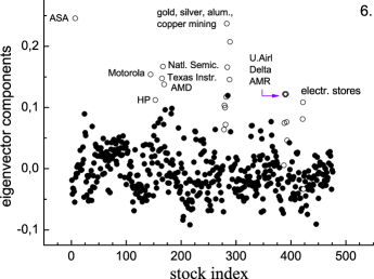
Figure 6: Component sizes of chosen eigenvectors. The number in each panel indicates the rank of the corresponding eigenvalue. Horizontal ordering is such that stocks belonging to same business sectors are next to each other and open symbols are used as a guide to the eye. For abbreviations, see text.

The highest ranking intermediate eigenvector, namely the second eigenvector is a good example of an eigenvector localized on a business sector. The components corresponding to the utilities sector stand out very cleanly in Fig. 6. One should notice, however, that this would not be the case without the chosen horizontal ordering of the companies. Without a priori information we would not be able to define boundaries for this cluster.

The third eigenvector, which is mainly localized on oil and gold & silver mining companies is already a more difficult one. The other large components of this eigenvector correspond to Petroleum & Resources (P&R), a financial company specialized in the energy sector, Tidewater (Tidew), which provides vessels and services for the offshore energy industry, and ASA Ltd. (ASA), an investment company interested in precious metal mining. The thresholding analysis (not presented here) shows that the companies corresponding to the largest components of this eigenvector form two clusters. The third eigenvector is not the only example of a high ranking intermediate eigenvector localized on more than one cluster. The sixth eigenvector, for example, is localized on gold & silver mining, leading electronics manufacturers & electronics stores, and air transportation companies. Again, the thresholding analysis shows that all these industries form their own clusters. Interestingly the seventh eigenvector is localized solely on the gold & silver mining-related companies.

One encounters further difficulties, when analyzing e.g. the tenth eigenvector, which has a very complex structure. As illustrated in Fig. 6, it is localized on a large number of industry branches, most of which can be found by the thresholding analysis. However, without some prior information, interpretation of this eigenvector is impossible. On the other hand, surprisingly, the 19th eigenvector can be straightforwardly interpreted although the corresponding eigenvalue is close to the random part of the spectrum ($\lambda_{19}\approx 0.55$) and the neighbouring eigenvectors are to a large extent random. This eigenvector is strongly localized on Sony and Honda, the only Japanese companies in the data set. It should be noted that several eigenvectors corresponding to the lowest ranking eigenvalues are localized on pairs of companies with highest correlation coefficients.

To summarize, it seems evident that the cluster structure of a network cannot be easily deduced from the eigenvectors of the weight matrix. Especially, interpretation of a single eigenvector is even more difficult than suggested in recent literature. Most of the information about the cluster structure can only be found by combining information from different eigenvectors. There is, however, no rule to tell, which linear combination of the eigenvectors should be taken. Therefore, the extraction of the cluster structure from the eigenvectors without a priori knowledge about the nodes (here companies) seems to be a too formidable task.

4.3 Diffusion based approach

In section 2.2 we reasoned, how the cluster structure of a network should affect the diffusion process. The spectrum of the diffusion matrix (depicted by the solid line in Fig. 7) has, as expected, similar structure with that of the weight matrix. For diffusion matrices, results corresponding to Eqs. (12) and (13) are not known, but a random reference function can be obtained numerically by constructing diffusion matrices from random weight matrices generated with the method presented in section 3.2 and in [42] (dashed line in Fig. 7).

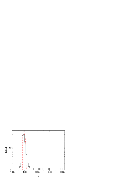
Figure 7: (Color online) Spectral density of the diffusion matrix corresponding to the larger dataset (solid line), and the average spectral density over a system of $1000$ random references (dashed line). The trivial eigenvalue at $0$ is not shown.

In Fig. 8 we compare the eigenvectors of the weight and diffusion matrices. We see that the highest ranking eigenvectors of the diffusion matrix are very close to the corresponding eigenvectors (i.e. eigenvectors with similar localization) of the weight matrix. Their distance increases when the random part of the spectrum is approached and the correspondence between pairs of eigenvectors looses its meaning.

Figure 8: Scalar products of the eigenvectors of the diffusion matrix and the corresponding eigenvectors (i.e. eigenvectors with similar localization) of the weight matrix. The eigenvectors of the diffusion matrix are ordered according to decreasing rank (x-axis).

The analysis of the eigenvectors of the normal matrix is again non-trivial. Naturally, there are correlations between the components of different eigenvectors, but it is impossible to identify clusters without a priori information. Best results in two dimensions were obtained with the eigenvectors of ranks two and five (see Fig. 9). Visual inspection of this plot allows us to identify the oil & gas, utilities and gold & silver mining clusters, although the determination of the boundaries is again difficult.

Figure 9: Components of the fifth eigenvector of the normal matrix as a function of the components of the second eigenvector.

5 Asset graph approach to the clustering of stocks

In this section we study the clustering of stocks using asset graphs [19]. An asset graph is constructed by ranking the non-diagonal elements of the correlation matrix and adding links between stocks one after the other, starting from the strongest correlation coefficient. The network thus emerging can be characterized by a parameter $p$, which is the ratio of the number of added links to the number of all possible links, $N(N-1)/2$. Asset graphs constructed using the full correlation matrix $\boldsymbol{C}$ are illustrated in Fig. 10 for link occupation values of $p=0.01$, $p=0.03$, $p=0.05$, and $p=0.07$. An immediate observation is that some clusters stand out very cleanly and can already be identified by visual inspection. These clusters correspond very well to business sectors and industries according to Forbes classification [45]. However, we cannot expect to find all clusters this way and for large $N$ this approach cannot be applied. It is clear that we need more sophisticated methods. One possibility, suggested by Onnela et al., is to define a cluster as an isolated component and study the evolution of these components as a function of $p$. Another possibility is to apply some known community detection method for binary graphs (see e.g. [7, 8, 35, 46, 47]) as a function of $p$. However, the problem with these approaches is that there is no global threshold value of $p$ with which we would find (almost) all the information about the clusters. A more comprehensive picture about the cluster structure can be obtained by studying the evolution of each cluster separately as a function of $p$. Alternatively, we can also define our asset graphs in a different way.

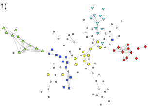
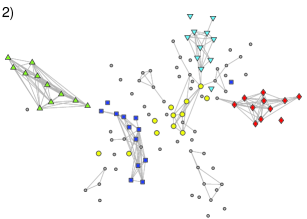
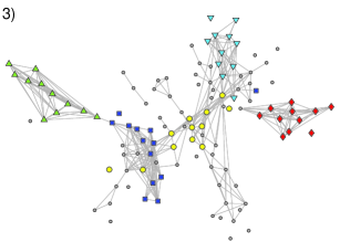
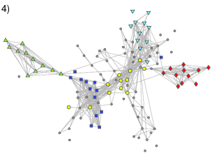
Figure 10: (color online) The asset graph constructed using the full correlation matrix $\boldsymbol{C}$ for link occupation values 1) $p=0.01$, 2) $p=0.03$, 3) $p=0.05$ and 4) $p=0.07$. Forbes classification [45] has been used and companies belonging to Energy sector are denoted by $\blacktriangle$, Electric Utilities industry by $\blacklozenge$, Healthcare sector by $\blacktriangledown$, Basic Materials sector by $\blacksquare$ and Finacial as well as Conglomerates sector by $\bullet$. Other nodes are denoted by $\bullet$.

The largest components of the market eigenvector, mostly conglomerates and financial companies, have significant correlations with almost all the other companies. This leads to the phenomenon clearly seen in Fig. 10 that different clusters in asset graphs merge mostly through nodes corresponding to these companies (for further discussion see [39]). Therefore, it is interesting to study asset graphs without the effect of the market eigenvector. This can be done by expanding the correlation matrix as

$$\boldsymbol{C}=\sum_{i=1}^{N}\lambda_{i}|e_{i}\rangle\langle e_{i}|,$$ (23)

where the eigenvalues are sorted according to decreasing rank and constructing the asset graphs using the matrix defined by

$$\boldsymbol{C}_{-m}=\sum_{i=2}^{N}\lambda_{i}|e_{i}\rangle\langle e_{i}|.$$ (24)

These are illustrated in Fig. 11 for link occupation values of $p=0.01$, $p=0.03$, $p=0.05$, and $p=0.07$.

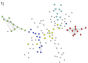
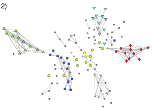
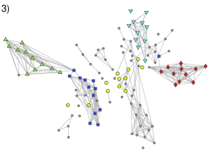
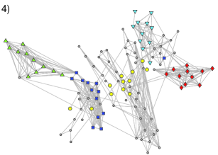
Figure 11: (color online) The asset graph constructed using $\boldsymbol{C}_{-m}$ (i.e. correlation matrix from which the effect of the market eigenpair has been filtered out) for link occupation values 1) $p=0.01$, 2) $p=0.03$, 3) $p=0.05$ and 4) $p=0.07$. Nodes are denoted as in Fig. 10.

Here the most significant difference compared to Fig. 10 is that, since the market eigenvector is excluded, the degrees of the nodes with the highest betweeness centralities in the MST (see Fig. $1$ in [20]) are much lower and some components remain isolated for larger values of $p$. However, from panel a of Fig. 14, where we illustrate as a function of $p$ the number of isolated components of size larger than one, as well as from Fig. 11 we notice that the problem still stands. There is no global threshold value of $p$ that would reveal all the clusters.

Kim et al. [39] have approached the problem by defining, what they call the group correlation matrix by

$$\boldsymbol{C}_{g}=\sum_{i=2}^{N_{g}}\lambda_{i}|e_{i}\rangle\langle e_{i}|,$$ (25)

where $N_{g}$ is used to exlude the effect of the random eigenpairs. From the previous section we know that by choosing $N_{g}<N$ we lose some information, but the idea here is to get rid of most of the noise without losing too much information. $N_{g}$ can be approximated by comparing the eigenvalues to the theoretical eigenvalue density for random correlation matrices and by studying the localization of the eigenvectors. In the following we have used $N_{g}=10$.

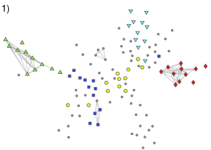
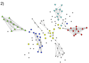
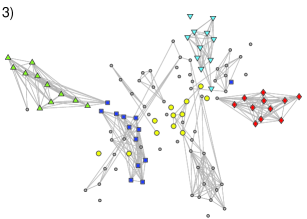
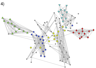
Figure 12: (color online) The asset graph constructed using $\boldsymbol{C}_{g}$ (i.e. correlation matrix from which the effects of the market and random eigenpairs has been filtered out) for link occupation values 1) $p=0.01$, 2) $p=0.03$, 3) $p=0.05$ and 4) $p=0.07$. Nodes are denoted as in Fig. 10.

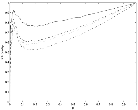
Figure 13: The fraction of overlapping (i.e. common) links in asset graphs constructed from $\boldsymbol{C}_{g}$ and $\boldsymbol{C}_{-m}$ (solid line), $\boldsymbol{C}$ and $\boldsymbol{C}_{-m}$ (dashed line), $\boldsymbol{C}$ and $\boldsymbol{C}_{g}$ (dotted line) and in all three (dashdotted line).

In Figure 12 we show asset graphs constructed using $\boldsymbol{C}_{g}$ for link occupation values of $p=0.01$, $p=0.03$, $p=0.05$, and $p=0.07$. We see that these graphs are very similar to those presented in Fig. 11, i.e., to the ones constructed by using $\boldsymbol{C}_{-m}$. This is verified in Fig. 13, which shows the fraction of overlapping links, i.e. the percentage of common links, in the studied asset graphs. The shape of the curves turns out to be interesting. In all cases the overlap increases very rapidly until $p\approx 0.025$. After this, the overlap decreases indicating that the links become more random, but as the number of links grows larger and the fraction of “free” places decreases, the overlap starts to increase again. As a reference, one can use Erdös-Rényi ensemble $G(m,N)$, which consists of graphs of $N$ nodes and exactly $m$ links, such that each possible graph appearing with equal probability. The overlap for $G(m,N)$ is clearly $p^{2}$.

The overlap between asset graphs constructed from $\boldsymbol{C}_{g}$ and $\boldsymbol{C}_{-m}$ is found to be around 93% for $p\approx 0.025$ and over 90% in the interval $[0.022,0.037]$. From panel a of Fig. 14, in which we show the number of isolated components as a function of $p$, one sees that this number is also at its highest in the interval, meaning that these are the most relevant values of $p$ when studying the clustering. This means that we do not gain much by filtering out the random eigenpairs before constructing the asset graphs. At the same time we may lose some significant information about the small clusters stored in the lowest ranking eigenpairs, as discussed in the previous section. One should notice that cluster identification is more difficult when the full correlation matrix is used, but the difference is not very large. When this is combined with the fact that most information about the financial and conglomerate companies is lost when the market eigenvector is filtered out, it is evident that best results are obtained by using both $\boldsymbol{C}$ and $\boldsymbol{C}_{-m}$.

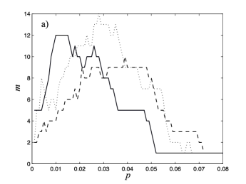
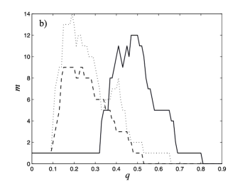
Figure 14: The number of isolated components $m$ as a function of $p$ (panel a) and $q$ (panel b) in asset graphs constructed from $\boldsymbol{C}$ (solid line), $\boldsymbol{C}_{g}$ (dashed line) and $\boldsymbol{C}_{-m}$ (dotted line). For $\boldsymbol{C}_{g}$ and $\boldsymbol{C}_{-m}$ there is a sudden increase at $q_{c}\approx 0.1$ (panel b). This jump, however, is not seen in panel a. (Notice that the number of links increases as a function of $p$ and decreases as a function of $q$.)

Kim et al. [39] have suggested that asset graphs constructed from $\boldsymbol{C}_{g}$ have a well-defined critical threshold $p_{c}$, where many isolated components merge into one giant component. They construct the asset graphs by including all the links that correspond to a correlation coefficient above a predetermined value $q$ and plot the number of isolated components as a function of $q$. A similar plot for the present data set is shown in panel b of Fig. 14. At the first sight it seems that there exists a clear critical threshold $q_{c}\approx 0.1$ (seen as a sudden jump in the number of components) for the asset graphs constructed from $\boldsymbol{C}_{g}$ but no clear threshold for those constructed from the full correlation matrix. However, it is perhaps a little misleading to speak about a critical threshold, since the one "seen" in panel b of Fig. 14 is due to the fact that the elements of $\boldsymbol{C}_{g}$ are not uniformly distributed. From panel a of Fig. 14 one sees that there is no clear threshold in none of these cases (as no sudden jumps are seen).

To summarize, it seems that the noise present in the time series does not change the cluster structure of the asset graphs, which is not very surprising since only links corresponding to the highest correlation coefficients are included. It also seems that there is no critical threshold $p_{c}$ in any of the studied cases. Therefore, useful information may be lost, while no benefit is gained, if the random eigenpairs are filtered out before constructing the asset graphs.

6 Summary

The aim of the present work was to investigate in complex systems the relationship between the spectral properties of correlation based matrices and the cluster structure of the related networks. The network was constructed as a complete graph where the weights were identified with elements taken from the correlation matrix. We have chosen to study stock market data since large amount of information has already been accumulated about them and their spectral properties have also been studied in detail [24, 25]. Two data sets from the NYSE were analyzed, one with lesser stocks appropriate for visualization and a larger one with better statistical properties.

We started our study by analyzing the eigenvector corresponding to the largest eigenvalue of the weight matrix and found to a very good first approximation that the eigenvector components correspond to the strengths of the nodes (i.e. companies). There is a systematic second order correction roughly proportional to the nodal strengths, which is probably due to the modular structure of the network.

The identification of the clusters using the high ranking eigenvectors turned out to be a too formidable task. Therefore, we have chosen a different path: Using independent information, we have given interpretations to typical eigenvectors. Our results show that there are eigenvectors which are well localized to a few industrial branches. Surprisingly, such eigenvectors are not have always high ranking i.e. correspond to a large eigenvalue. On the other hand, some high rank eigenvectors represent so many branches that they are hardly distinguishable from the random case. Therefore, we think that the eigenvectors are not appropriate in identifying the modules of such networks. By using the diffusion matrix we had to arrive to a similar conclusion, though it should be emphasized that there is a strong overlap between the highest ranking eigenvectors of the weight and diffusion matrices.

Since direct network methods are known to be efficient in identifying the hierarchical structure of correlation based networks [13, 17, 19, 21], we have studied how the spectral methods can be combined with the asset graph method based on thresholding. We have compared the asset graphs as obtained from the noisy and denoised correlation matrices, where denoising was carried out by using spectral information [39]. It turned out that denoising has little effect on the clusters of asset graphs. This is because of the hierarchical structure of the clusters and due to the fact that thresholding picks the high correlations where the noise is expected to play a subordinate role. Surprisingly enough similar denoising methods seem to work efficiently when applied directly to portfolio optimization [42].

We can conclude that the identification of clusters or communities is even more difficult in the case of highly connected weighted networks. Spectral methods may lead to an overall description of the properties of complex systems but they do not seem to be appropriate for the classification problem without additional information about the nodes of the related network.

7 Acknowledgements

TH, JS and KK are supported by the Academy of Finland (The Finnish Center of Excellence program 2006-2011). JK and GT were partially supported by OTKA K60456.

References

- [1] M.E.J Newman, A.-L. Barabási, D.J. Watts, The Structure and Dynamics of Networks, Princeton University Press (2006).
- [2] S.N. Dorogovtsev, J.F.F. Mendes, Evolution of Networks: From Biological Nets to the Internet and WWW, Oxford University Press (2003).
- [3] M.E.J. Newman, SIAM Review 45, 167 (2003).
- [4] G. Caldarelli, Scale Free Networks, Oxford University Press (2007).
- [5] S.S. Shen-Orr, R. Milo, S. Mangan, U. Alon, Nature Genetics 31, 64 (2002).
- [6] J.-P. Onnela, J. Saramäki, J. Kertész, K. Kaski, Physical Review E 71, 065103(R) (2005).
- [7] M.E.J. Newman, M. Girvan, Phys. Rev. E 69, 026113 (2004).
- [8] G. Palla, I. Derényi, I. Farkas, and T. Vicsek, Nature 435, 814 (2005)
- [9] J.-P. Onnela, J. Saramäki, J. Hyvönen, G. Szabó, D. Lazer, K. Kaski, J. Kertész, A.-L. Barabási, Proceedings of the National Academy of Sciences (USA) 104, 7332 (2007).
- [10] H. Markowitz, The Journal of Finance 7, 77 (1952).
- [11] J.-P. Bouchaud, M. Potters, Theory of Financial Risk and Derivative Pricing; From Statistical Physics to Risk Management, Cambridge University Press (2003).
- [12] R.S. Tsay, Analysis of Financial Time Series, John Wiley (2002).
- [13] R.N. Mantegna, European Physical Journal B 11, 193 (1999).
- [14] G. Bonanno, N. Vandewalle and R.N. Mantegna, Physical Review E 62, 7615 (2000).
- [15] G. Bonanno, G. Caldarelli, F. Lillo and R.N. Mantegna, Physical Review E 68, 046130 (2003).
- [16] G. Bonanno, G. Caldarelli, F. Lillo, S. Miccichè, N. Vandewalle and R.N. Mantegna, European Physical Journal B 38, 363 (2004).
- [17] J.-P. Onnela, A. Chakraborti, K. Kaski, J. Kertész and A. Kanto, Physical Review E 68, 056110 (2003).
- [18] J.-P. Onnela, A. Chakraborti, K. Kaski, J. Kertész and A. Kanto, Physica Scripta T38, 48 (2003).
- [19] J.-P. Onnela, K. Kaski, J. Kertész, European Physical Journal B 38, 353 (2004).
- [20] T. Heimo, J. Saramäki, J.-P. Onnela, K. Kaski, Physica A 383, 147 (2007).
- [21] M. Tumminello, T. Aste, T. Di Matteo, R.N. Mantegna, Proceedings of the National Acadademy of Sciences (USA) 102, 10421 (2005).
- [22] L. Kullmann, J. Kertész, R.N. Mantegna, Physica A 287, 412 (2000).
- [23] L. Giada, M. Marsili, Physical Review E 63, 061101 (2001).
- [24] L. Laloux, P. Cizeau, J.-P. Bouchaud, and M. Potters, Physical Review Letters 83, 1467 (1999).
- [25] V. Plerou, P. Gopikrishnan, B. Rosenow, L.A.N. Amaral, H.E. Stanley, Physical Review Letters 83, 1471 (1999).
- [26] V. Plerou, P. Gopikrishnan, B. Rosenow, L.A.N. Amaral, T. Guhr, H.E. Stanley, Physical Review E 65, 066126 (2002).
- [27] Z. Burda, J. Jurkiewicz, M.A. Nowak Acta Physica Polonica B34, 87 (2003).
- [28] A. Barrat, M. Barthélemy, R. Pastor-Satorras, A. Vespignani, Proceedings of the National Academy of Sciences (USA) 101, 3747 (2004).
- [29] J. Scott, Social Network Analysis: A Handbook, 2nd ed., Sage (2000).
- [30] B. Bollobás, Random Graphs, Cambridge University Press (2001).
- [31] K.A Eriksen, I. Simonsen, S. Maslov, K. Sneppen, Physical Review Letters 90 148701 (2003).
- [32] I. Simonsen, K.A. Eriksen, S. Maslov, K. Sneppen, Physica A 336, 163 (2004) .
- [33] I. Simonsen, Physica A 357, 317 (2005).
- [34] R. Guimera, L.A.N. Amaral, Nature 433, 895 (2005).
- [35] J. Reichardt, S. Bornholdt, Phys. Rev. Lett. 93, 218701 (2004).
- [36] S. Fortunato, M. Barthélemy, Proceedings of the National Academy of Sciences (USA) 104, 36 (2007).
- [37] J. Kumpula, J. Saramäki, K. Kaski, J. Kertész, European Physical Journal B 56, 41 (2007).
- [38] P. Gopikrishnan, B. Rosenow, V. Plerou, H. E. Stanley, Physical Review E 64, 035106 (2001).
- [39] D.-H. Kim, H. Jeong, Physical Review E 72, 046133 (2005).
- [40] V.A. Marchenko, L.A. Pastur, Math. USSR-Sbornik, 1 457 (1967).
- [41] Yahoo Finance at http://finance.yahoo.com, referenced in August 2006.
- [42] S. Pafka, I. Kondor, Physica A 319, 487 (2003).
- [43] A. Utsugi, K. Ino, M. Oshikawa, Physical Review E 70, 026110 (2004).
- [44] Z. Burda, A. T. Görlich, B. Waclaw, Physical Review E 74, 041129 (2006).
- [45] Forbes at http://www.forbes.com, referenced in March-April 2002.
- [46] J. Reichardt, S. Bornholdt, Physical Review E 74, 016110 (2006).
- [47] M.E.J. Newman, European Physical Journal B 38, 321 (2004).