Simulation Results for $U(1)$ Gauge Theory on Non-Commutative Spaces

Abstract:

We present numerical results for $U(1)$ gauge theory in 2d and 4d spaces involving a non-commutative plane. Simulations are feasible thanks to a mapping of the non-commutative plane onto a twisted matrix model. In $d=2$ it was a long-standing issue if Wilson loops are (partially) invariant under area-preserving diffeomorphisms. We show that non-perturbatively this invariance breaks, including the subgroup $SL(2,R)$. In both cases, $d=2$ and $d=4$, we extrapolate our results to the continuum and infinite volume by means of a Double Scaling Limit. In $d=4$ this limit leads to a phase with broken translation symmetry, which is not affected by the perturbatively known IR instability. Therefore the photon may survive in a non-commutative world.

1 Non-commutative $U(1)$ gauge theory

The positions in a non-commutative (NC) Euclidean plane correspond to the spectra of Hermitian operators $\hat{x}_{1},\ \hat{x}_{2}$, with a non-vanishing commutator

$$[\hat{x}_{\mu},\hat{x}_{\nu}]=i\Theta_{\mu\nu}=i\theta\epsilon_{\mu\nu}\ .$$ (1)

We treat the non-commutativity parameter $\theta$ as a constant. Relation (1) implies a spatial uncertainty of the form $\Delta x_{1}\Delta x_{2}\sim\theta$, which can be interpreted as the event horizon of a strong gravitation centre. In fact, if it has been argued that attempts to merge quantum theory with gravity lead quite generally to such a spatial uncertainty [2], which corresponds to a NC geometry.

In quantum field theory the spatial uncertainty gives rise to non-locality over a range of $O(\sqrt{\theta})$. A related consequence is the notorious “UV/IR mixing” [3]: nested singularities can be UV divergent in one momentum component $p_{\mu}$ and IR divergent in another component $p_{\nu}$. Due to this property the perturbative treatment is extremely involved.

Hence it is strongly motivated to take a fully non-perturbative approach. As in commutative field theory it relies on the lattice regularisation (for a review, see Ref. [4]). Although we do not have sharp points as lattice sites, a (fuzzy) lattice structure can be imposed by the operator identity

$$\exp\Big{(}i\frac{2\pi}{a}\hat{x}_{\mu}\Big{)}=\hat{1\!\!\!1}\ ,$$ (2)

where $a$ is the lattice spacing. Along with the usual periodicity of the momenta over the Brillouin zone, identity (2) entails $\frac{1}{2a}\theta p_{\mu}\in Z\!\!\!Z\ .$ For fixed parameters $a$ and $\theta$ we infer that the lattice is automatically periodic, in striking contrast to the commutative lattice.

On a periodic $N\times N$ lattice one readily identifies

$$\theta=\frac{1}{\pi}Na^{2}\ .$$ (3)

Therefore we extrapolate to the Double Scaling Limit (DSL)

$$\{\quad a\to 0\quad{\rm and}\quad N\to\infty\quad\}\qquad{\rm at}\quad Na^{2}={\rm const.}$$ (4)

The DSL leads to a continuous NC plane of infinite extent. The requirement to take the UV and IR limits simultaneously in a controlled manner is again related to the UV/IR mixing.

We can return to ordinary coordinates $x_{\mu}$ if we multiply all fields by star products,

$$\phi(x)\star\psi(x):=\phi(x)\exp\Big{(}\frac{i}{2}\mathop{\raise 6.02773pt\hbox{$\leftarrow$\kern-7.5pt\raise-6.02773pt\hbox{$\partial$}}}\ \!\!\!_{\mu}\Theta_{\mu\nu}\!\mathop{\raise 6.02773pt\hbox{$\rightarrow$\kern-8.00003pt\raise-6.02773pt\hbox{$\partial$}}}\ \!\!\!_{\nu}\Big{)}\psi(x)\ ,$$ (5)

which encode the non-locality. The star commutator $[x_{\mu},x_{\nu}]_{\star}:=x_{\mu}\star x_{\nu}-x_{\nu}\star x_{\mu}=i\Theta_{\mu\nu}$ suggests that this transition is sensible — it can be justified e.g. with a plane wave decomposition.

In this framework we formulate $U(1)$ gauge theory on a NC plane as

$$S[A]=\frac{1}{4}\int d^{2}x\ F_{\mu\nu}\star F_{\mu\nu}\ ,\quad F_{\mu\nu}=\partial_{\mu}A_{\nu}-\partial_{\nu}A_{\mu}+ig[A_{\mu},A_{\nu}]_{\star}\ .$$ (6)

Note that even the $U(1)$ gauge field picks up a self-interaction term. This action is invariant under star gauge transformations. However, even on the lattice its direct simulation is hardly feasible (for instance the compact formulation would require star unitary link variables).

We arrive at a numerically tractable formulation based on the equivalence of this model with the twisted Eguchi-Kawai (TEK) model [5]. This matrix model is defined on one point with the action

$$S_{\rm TEK}[U]=-N\beta\sum_{\mu\neq\nu}Z_{\mu\nu}{\rm Tr}[U_{\mu}U_{\nu}U_{\mu}^{\dagger}U_{\nu}^{\dagger}]\quad,\qquad\beta\equiv 1/g^{2}\ .$$ (7)

The $U_{\mu}$ are unitary $N\times N$ matrices, which contain the degrees of freedom of the lattice gauge field. The twist factor $Z_{21}=Z_{12}^{*}=\exp(2\pi in/N)$ makes the difference from the original Eguchi-Kawai model — in $d=4$ it avoids the spontaneous breaking of the centre symmetry at weak coupling. $n$ is an integer, which we set $n=(N+1)/2$, so we always deal with odd matrix/lattice sizes $N$.

Then the TEK can be identified with the NC $U(1)$ lattice gauge model since the algebras are identical — this has been shown in the large $N$ limit [6] and also at finite $N$ [7]. Clearly, the TEK is numerically tractable, so that the simulations can start if we also formulate suitable observables. In the matrix model framework it is obvious to write down the analogue of a Wilson loop,

$$W_{\mu\nu}(I\times J):=\frac{1}{N}\,Z_{\mu\nu}^{I\cdot J}\,{\rm Tr}[U_{\mu}^{I}U_{\nu}^{J}U_{\mu}^{\dagger\,I}U_{\nu}^{\dagger\,J}]\ .$$ (8)

Mapping this quantity back to the lattice yields indeed the star gauge invariant term, which is considered the NC Wilson loop [8]. This Wilson loop is complex in general, $W_{\mu\nu}\in{\kern 2.5pt\sf{C}\kern-4.49997pt\sf{{\small{I}}}\kern 4.49997pt\kern-2.5pt}$, but the action is real since both orientations are summed over (and $W_{\mu\nu}=W_{\nu\mu}^{*}$). Hence simulations are possible without running into a sign problem. Such a study, including extrapolations to the DSL, was first presented in Ref. [9]. The planar limit coincides with $U(N\to\infty)$ lattice field theory, where the (real) Wilson loop follows an exact area law [10]. Although this is not the limit that we are interested in, it can be used to set the scale as $a^{2}=-\ln[1-1/(4\beta)]$  (for $\beta\geq 1/2$), so that the DSL has to be taken roughly at a fixed ratio $N/\beta$.

2 Wilson loops in $d=2$ : area-preserving diffeomorphisms (APDs)

On the commutative plane, pure $U(n)$ gauge theories are analytically soluble with geometric methods. Due to APD invariance, the expectation values of Wilson loops only depend on the oriented area [11].

Contrary to original expectations, it turned out that this symmetry does not hold on the NC plane. In particular, perturbation theory to $O(g^{4})$ and $O(\theta^{-2})$ revealed that it breaks down to $SL(2,R)$ [12], in agreement with other considerations [13]. By means of numerical simulations we investigated the non-perturbative extent of this APD symmetry breaking, as well as the viability of the subgroup $SL(2,R)$ [14]. To this end, we considered four types of non-intersecting Wilson loops with polygonal boundaries, generalising the form (8). Prototypes are depicted in Figure 1.

Figure 1: Examples for squares, L-shapes, rectangles and stairs, the four types of Wilson loops that we measured at the same area to investigate the behaviour under APD transformation, cf. Figure 2.

Figure 2 shows results for a set of Wilson loops at $N=125$, $\beta=3.91$ (on the left) and $N=155$, $\beta=4.82$ (on the right). In both cases the non-commutativity parameter amounts to $\theta=2.63$, hence we see two snapshots on the way to the DSL: the right-hand-side corresponds to a larger volume with a finer lattice. For a fixed (dimensional) loop area the results are very similar, hence we have apparently reached the asymptotic DSL behaviour. At small areas we observe agreement with the Gross-Witten area law [10] (and therefore with the planar limit) for all shapes. On the other hand, at larger areas $|\langle W\rangle|$ does not decay further and the values for the different shapes drift apart. This shows the extent of APD symmetry breaking, which seems to persist in the DSL to the continuum and infinite volume.

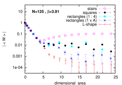
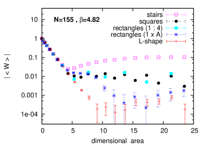
Figure 2: Absolute Wilson loop values of different shapes for two volumes and lattice spacing at $\theta=2.63$. The good agreement between the two plots indicates that the APD symmetry breaking persists in the DSL.

The rectangles (including squares) are related by the APD subgroup $SL(2,R)$. In fact, $SL(2,R)$ has a higher viability as an approximate symmetry subgroup — at least up to moderate deformations — but it also breaks on the non-perturbative level.

3 The fate of the photon in a non-commutative world

We consider again a NC plane with $[\hat{x}_{1},\hat{x}_{2}]=i\theta={\rm const.}$, but now we add a commutative plane $(x_{3},x_{4})$, which includes the Euclidean time. We are particularly interested in a possible $\theta$-distorted dispersion relation of the photon, which could in principle be experimentally measurable. A one loop calculation suggests the form [15]

$$E^{2}=\vec{p}^{\,2}+\frac{C}{\tilde{p}_{\mu}\tilde{p}_{\mu}}\qquad{\rm where}\quad C={\rm const.}\ ,\quad\tilde{p}_{\mu}:=\Theta_{\mu\nu}p_{\nu}\ .$$ (9)

Corresponding phenomenological data have been analysed, in particular in view of the time of flight of cosmic photons in Gamma Ray Burst (GRBs). In a GRB photons over a range of about $10^{5}\dots 10^{8}$ eV are emitted within a few seconds or minutes from a small source. In particular, evaluating the times of photon arrival for 35 GRBs against the dispersion ansatz $E=|\vec{p}|+E/M$ (where $M$ is a large mass due to some “quantum gravity foam”), Ref. [16] concluded $M>0.001M_{\rm Planck}$. It has been proposed to establish a bound on $\|\Theta\|$ by similar considerations [17], which should address the IR singularity in eq. (9). However, the constant $C$ turned out to be negative to one loop [18], which suggested that NC QED is IR unstable and thus ill-defined. In Ref. [19] we revisited NC QED non-perturbatively: we discretised the commutative plane with an $L\times L$ lattice and the NC plane with a TEK model of matrix size $N\approx L$. A physical scale was identified by matching Wilson loop expectation values (and further observable) at different $\beta$ values. To a good approximation this led to $a\propto 1/\beta$, so that the DSL is taken at fixed $\,\theta\propto N/\beta^{2}\,$ (unlike NC QED₂), see Figure 3.

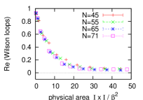
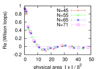
Figure 3: Results for Wilson loop in NC QED₄ at $N/\beta^{2}\equiv 20$ in the commutative plane, the mixed plane and the NC plane (from left to right). In the first two planes $\langle W\rangle$ is real, whereas the oscillation of ${\rm Re}\,\langle W\rangle$ comes along with a rotating complex phase (similar to NC QED₂ [9]).

As an order parameter for translation symmetry in the NC plane we measured the open Polyakov line, which is $\star$-gauge invariant and which carries momentum $p$,

$$P_{\mu}(n)={\cal P}\exp_{\star}\Big{(}ig\int_{x}^{x+\tilde{p}_{\mu}}A_{\mu}(\xi)\,d\xi_{\mu}\Big{)}\ ,\qquad{\cal P}~{}:~{}{\rm path~{}ordering},~{}\tilde{p}_{\mu}=na\hat{\mu}~{}:~{}{\rm length}\ .$$ (10)

Figure 4 shows the (expected) symmetric phases at strong and at weak coupling, but a broken phase above $\beta\simeq 0.35$. The upper end of the broken phase rises roughly $\propto N^{2}$, and its hysteresis behaviour implies that the corresponding phase transition is of first order.

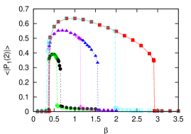
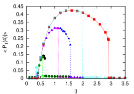
Figure 4: The expectation values of open Polyakov lines of length $2a$ (on the left) and $4a$ (on the right) for $N=15,\ 25$ and $35$ (curves from left to right, with hysteresis at the transition to the weak coupling phase). At intermediate gauge coupling we recognise a phase of broken translation symmetry.

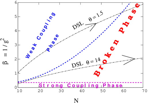
Figure 5: The phase diagram for QED₄ with a NC plane: between the strong coupling phase ($\beta<0.35$) and the weak coupling phase we find a phase of broken translation invariance. Since the weak/broken transition rises like $\beta\propto N^{2}$, whereas the DSL for a fixed NC parameter $\theta$ follows $\beta\propto\sqrt{N}$, the DSL always ends up in the broken phase.

This leads to the phase diagram 5, where we also mark the trajectories for DSLs with different values of $\theta$. These DSL curves always lead to the broken phase, where we observe IR stability of all observables measured [19]. The perturbative result describes correctly the weak coupling phase, as the dispersion relation (in the commutative plane) in Figure 6 on the left shows. The plot on the right refers to the broken phase, which captures the physically relevant DSL. Here the photon dispersion is linear, and the photon can be identified with the Nambu-Goldstone boson of spontaneous translation symmetry breaking.

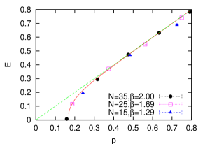
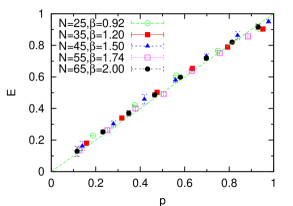
Figure 6: Dispersion relations $\,E(p)\$ for the photon in a NC space in the weak coupling phase (on the left, $p=p_{1}$), and in the broken phase (on the right, $p=p_{3}$). The former result is consistent with the perturbatively predicted IR instability (“tachyonic” behaviour, eq. (3.1) with $C\simeq 0.1285$). In the physical phase the photon is massless again, corresponding to a Nambu-Goldstone boson of the broken translation symmetry.

4 Conclusions

We simulated QED₂ and QED₄ on spaces containing a NC plane. In both cases we observed a stable behaviour in the DSL to a continuous NC space of infinite extent, which suggests renormalisability. UV/IR mixing is manifest as a non-perturbative effect, in agreement with numerical DSL results for the 3d NC $\lambda\phi^{4}$ model [24].

$\bullet$ In $d=2$ the APD invariance of Wilson loops breaks, without any residual subgroup. Hence there is hardly hope for an analytic solution, but we may hope for a rich structure to be explored numerically [9, 14].

$\bullet$ In $d=4$ the DSL leads to a phase of intermediate coupling strength and broken translation symmetry. This physical phase appears to be IR stable — in contrast to the weak coupling phase. Therefore the NC space may accommodate photons after all [19].

Acknowledgement : This work was supported by the DFG, HPC-Europe, INFN and D.O.E. under cooperative research agreement DE-FG02-05ER41360. The computations were performed in part on parallel machines at HLRN and HLRS, and on a PC cluster at Humboldt-Universität.

References

- [1]
- [2] S. Doplicher, K. Fredenhagen and J.E. Roberts, Commun. Math. Phys. 172 (1995) 187.
- [3] S. Minwalla, M. Van Raamsdonk and N. Seiberg, JHEP 02 (2000) 020.
- [4] R.J. Szabo, Phys. Rept. 378 (2003) 207.
-
[5]
A. González-Arroyo and M. Okawa,
Phys. Rev. 27D (1983) 2397.
A. González-Arroyo and C.P. Korthals Altes, Phys. Lett. B131 (1983) 396. - [6] H. Aoki, N. Ishibashi, S. Iso, H. Kawai, Y. Kitazawa and T. Tada, Nucl. Phys. B565 (2000) 176.
- [7] J. Ambjørn, Y. Makeenko, J. Nishimura and R.J. Szabo, JHEP 11 (1999) 29; Phys. Lett. B480 (2000) 399; JHEP 05 (2000) 023.
- [8] D.J. Gross, A. Hashimoto and N. Itzhaki, Adv. Theor. Math. Phys. 4 (2000) 893.
- [9] W. Bietenholz, F. Hofheinz and J. Nishimura, JHEP 09 (2002) 9. H. Markum et al., theses proc.
- [10] D.J. Gross and E. Witten, Phys. Rev. D21 (1980) 446.
- [11] E. Witten, Commun. Math. Phys. 141 (1991) 153.
-
[12]
J. Ambjørn, A. Dubin and Y. Makeenko,
JHEP 0407 (2004) 044.
A. Bassetto, G. De Pol, A. Torrielli and F. Vian, JHEP 05 (2005) 061. -
[13]
M. Cirafici, L. Griguolo, D. Seminara
and R.J. Szabo,
JHEP 0510 (2005) 030.
M. Riccardi and R.J. Szabo, hep-th/0701273. - [14] W. Bietenholz, A. Bigarini and A. Torrielli, JHEP 08 (2007) 041.
- [15] A. Matusis, L. Susskind and N. Toumbas, JHEP 0012 (2000) 002.
- [16] J.R. Ellis et al., Astropart. Phys. 25 (2006) 402.
- [17] G. Amelino-Camelia et al., Nature 393 (1998) 763.
- [18] K. Landsteiner, E. Lopez and M.H.G. Tytgat, JHEP 0106 (2001) 055; Z. Guralnik et al., JHEP 0205 (2002) 025. F. Ruiz Ruiz, Phys. Lett. B502 (2001) 274. A. Bassetto et al., JHEP 0107 (2001) 008.
- [19] W. Bietenholz, J. Nishimura, Y. Susaki and J. Volkholz, JHEP 10 (2006) 042; arXiv:0706.3244.
- [20] T. Ishikawa and M. Okawa, talk presented at the annual meeting of the Japanese Physical Socienty, Sendai (2003). See also T. Ishikawa, T. Azeyanagi, M. Hanada and T. Hirata, these proceedings.
- [21] M. Teper and H. Vairinhos, hep-th/0612097, and these proceedings.
- [22] D. Colladay and V.A. Kostelecký, Phys. Rev. D58 (1998) 116002.
- [23] S.M. Carroll et al., Phys. Rev. Lett. 87 (2001) 141601.
- [24] W. Bietenholz, F. Hofheinz and J. Nishimura, JHEP 06 (2004) 042.