Dark energy and cosmic curvature: Monte-Carlo Markov Chain approach

Abstract

We use the Monte-Carlo Markov Chain method to explore the dark energy property and the cosmic curvature by fitting two popular dark energy parameterizations to the observational data. The new 182 gold supernova Ia data and the ESSENCE data both give good constraint on the DE parameters and the cosmic curvature for the dark energy model $w_{0}+w_{a}z/(1+z)$. The cosmic curvature is found to be $|\Omega_{k}|\lesssim 0.03$. For the dark energy model $w_{0}+w_{a}z/(1+z)^{2}$, the ESSENCE data gives better constraint on the cosmic curvature and we get $|\Omega_{k}|\leq 0.02$.

1 Introduction

The supernova (SN) Ia observations indicate the accelerated expansion of the Universe (Riess et al., 1998; Perlmutter et al., 1999). The direct and model independent evidence of the acceleration of the Universe was shown by using the energy conditions in Gong & Wang (2007b) and Gong et al. (2007). The driving force of the late time acceleration of the Universe, dubbed “dark energy (DE)”, imposes a big challenge to theoretical physics. Although the cosmological constant is the simplest candidate of DE and consistent with current observations, other possibilities are also explored due to many orders of magnitude discrepancy between the theoretical estimation and astronomical observations for the cosmological constant. For a review of DE models, see for example, Sahni & Starobinsky (2000); Padmanabhan (2003); Peebles & Ratra (2003); Sahni (2005); Copeland et al. (2006).

There are model independent studies on the nature of DE by using the observational data. In particular, one usually parameterizes DE density or the equation of state parameter $w(z)$ of DE (Alam et al., 2004a, b; Astier, 2001; Barger et al., 2007; Cardone et al., 2004; Chevallier & D. Polarski, 2001; Choudhury & Padmanabhan, 2005; Clarkson et al., 2007; Corasaniti & Copeland, 2003; Efstathiou, 1999; Gerke & Efstathiou, 2002; Gong, 2005a, b; Gong & Zhang, 2005; Gong & Wang, 2006, 2007a; Gu & Khlopov, 2007; Huterer & Turner, 2001; Huterer & Cooray, 2005; Ichikawa et al., 2006; Ichikawa & Takahashi, 2006, 2007; Jassal et al., 2005; Jönsson et al., 2004; Lee, 2005; Linder, 2003; Setare et al., 2007; Sullivan et al., 2007; Wang, 2000; Wang & Mukherjee, 2004; Wang & Tegmark, 2004; Weller & Albrecht, 2001, 2002; Wetterich, 2004; Zhu et al., 2004). Due to the degeneracies among the parameters in the model, complementary cosmological observations are needed to break the degeneracies. The Wilkinson Microwave Anisotropic Probe (WMAP) measurement on the Cosmic Microwave Background (CMB) anisotropy, together with the SN Ia observations provide complementary data. In this paper, we use the three-year WMAP (WMAP3) data (Spergel et al., 2007), the SN Ia data (Riess et al., 2006; Wood-Vasey et al., 2007; Davis et al., 2007) and the Baryon Acoustic Oscillation (BAO) measurement from the Sloan Digital Sky Survey (Eisenstein et al., 2005) to study the property of DE and the cosmic curvature. Two DE models $w(z)=w_{0}+w_{a}z/(1+z)$ (Chevallier & D. Polarski, 2001; Linder, 2003) and $w(z)=w_{0}+w_{a}z/(1+z)^{2}$ (Jassal et al., 2005) are considered. In Elgarøy & Multamäki (2007), the authors showed that combining the shift parameters $R$ and the angular scale $l_{a}$ of the sound horizon at recombination appears to be a good approximation of the full WMAP3 data. Wang and Mukherjee gave model independent constraints on $R$ and $l_{a}$ by using the WMAP3 data, they also provided the covariance matrix of the parameters $R$, $l_{a}$ and $\Omega_{b}h^{2}$ (Wang & Mukherjee, 2007). So we use the shift parameter $R$, the angular scale $l_{a}$ of the sound horizon at recombination and their covariance matrix given in Wang & Mukherjee (2007) instead to avoid using several inflationary model parameters and calculating the power spectrum. When the covariance matrix is used, we have six parameters. We use the Monte-Carlo Markov Chain (MCMC) method to explore the parameter space. Our MCMC code is based on the publicly available package COSMOMC (Lewis & Bridle, 2002).

The paper is organized as follows. In section II, we give all the formulae and show the constraint on the cosmic curvature is much better by using the parameters $R$, $l_{a}$ and their covariance matrix than that by using the parameter $R$ only. We also discuss the effect of the radiation component $\Omega_{r}$ on $l_{a}$. In section III, we give our results. We discuss the analytical marginalization over $H_{0}$ in appendix A.

2 Method

For the SN Ia data, we calculate

$$\chi^{2}=\sum_{i}\frac{[\mu_{obs}(z_{i})-\mu(z_{i})]^{2}}{\sigma^{2}_{i}},$$ (1)

where the extinction-corrected distance modulus $\mu(z)=5\log_{10}[d_{L}(z)/{\rm Mpc}]+25$, $\sigma_{i}$ is the total uncertainty in the SN Ia data, and the luminosity distance is

$$d_{\rm L}(z)=\frac{1+z}{H_{0}\sqrt{|\Omega_{k}|}}{\rm sinn}\left[\sqrt{|\Omega_{k}|}\int_{0}^{z}\frac{dz^{\prime}}{E(z^{\prime})}\right],$$ (2)

here

$$\frac{{\rm sinn}(\sqrt{|\Omega_{k}|}x)}{\sqrt{|\Omega_{k}|}}=\left\{\begin{array}[]{lr}\sin(\sqrt{|\Omega_{k}|}x)/\sqrt{|\Omega_{k}|},&{\rm if}\ \Omega_{k}<0,\\ x,&{\rm if}\ \Omega_{k}=0,\\ \sinh(\sqrt{|\Omega_{k}|}x)/\sqrt{|\Omega_{k}|},&{\rm if}\ \Omega_{k}>0,\end{array}\right.$$ (6)

and the dimensionless Hubble parameter is

$$E^{2}(z)=H^{2}(z)/H^{2}_{0}=\Omega_{m}(1+z)^{3}+\Omega_{r}(1+z)^{4}+\Omega_{k}(1+z)^{2}+\Omega_{DE},$$ (7)

where $\Omega=8\pi G\rho/(3H^{2}_{0})$, $\rho_{r}=\sigma_{b}T_{cmb}^{4}$, $\sigma_{b}$ is the Stefan-Boltzmann constant, the CMB temperature $T_{cmb}=2.726$K, and $\Omega_{DE}$ is the DE density. Note that the distance normalization is arbitrary in the SN Ia data, the Hubble constant $H_{0}$ determined from the SN data is also an arbitrary number, not the observed Hubble constant. Therefore we need to marginalize over this nuisance parameter $H_{0}$. The parameter $H_{0}$ is marginalized over with flat prior, the analytical marginalization method is discussed in Appendix A. For the DE model (Chevallier & D. Polarski, 2001; Linder, 2003)

$$w(z)=w_{0}+\frac{w_{a}z}{1+z},$$ (8)

the dimensionless DE density is

$$\Omega_{DE}(z)=(1-\Omega_{m}-\Omega_{k}-\Omega_{r})(1+z)^{3(1+w_{0}+w_{a})}\exp[-3w_{a}z/(1+z)].$$ (9)

For the DE model (Jassal et al., 2005)

$$w(z)=w_{0}+\frac{w_{a}z}{(1+z)^{2}},$$ (10)

the dimensionless DE density is

$$\Omega_{DE}(z)=(1-\Omega_{m}-\Omega_{k}-\Omega_{r})(1+z)^{3(1+w_{0})}\exp\left[3w_{a}z^{2}/2(1+z)^{2}\right].$$ (11)

For the SDSS data, we add the term

$$\left[\frac{A-0.469(0.95/0.98)^{-0.35}}{0.017}\right]^{2}$$

to $\chi^{2}$ (Eisenstein et al., 2005; Spergel et al., 2007), where the BAO parameter

$$A=\frac{\sqrt{\Omega_{m}}}{0.35}\left[\frac{0.35}{E(0.35)}\frac{1}{|\Omega_{k}|}{\rm sinn}^{2}\left(\sqrt{|\Omega_{k}|}\int_{0}^{0.35}\frac{dz}{E(z)}\right)\right]^{1/3}.$$ (12)

For WMAP3 data, we first add the term

$$\left(\frac{R-1.71}{0.03}\right)^{2}$$

to $\chi^{2}$ (Wang & Mukherjee, 2007), where the shift parameter

$$R=\frac{\sqrt{\Omega_{m}}}{\sqrt{|\Omega_{k}|}}{\rm sinn}\left(\sqrt{|\Omega_{k}|}\int_{0}^{z_{ls}}\frac{dz}{E(z)}\right),$$ (13)

and $z_{ls}=1089\pm 1$.

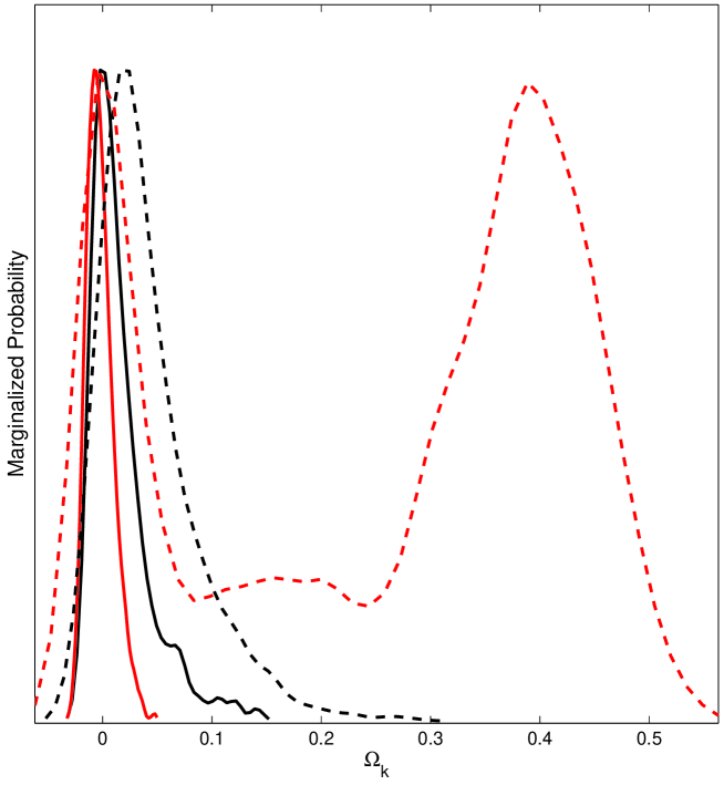
Figure 1: The marginalized probabilities of $\Omega_{k}$. The solid lines denote the results using the shift parameter $R$, the angular scale $l_{a}$, and the full covariance matrix. The dashed lines denote the results using the shift parameter only. The black lines are for the dark energy model $w_{0}+w_{a}z/(1+z)^{2}$ and the red lines are for the model $w_{0}+w_{a}z/(1+z)$.

When we fit the DE models (8) and (10) to the observational data, we have four parameters $\Omega_{m}$, $\Omega_{k}$, $w_{0}$ and $w_{a}$. The MCMC method is used to explore the parameter space. The marginalized probability of $\Omega_{k}$ is shown in Fig. 1. It is obvious that the cosmic curvature cannot be well constrained for the DE model (8). As discussed in Elgarøy & Multamäki (2007) and Wang & Mukherjee (2007), the combination of the shift parameter and the angular scale of the sound horizon at recombination gives much better constraints on cosmological parameters. So we add the angular scale of the sound horizon at recombination (Wang & Mukherjee, 2007)

$$l_{a}=\frac{\pi R/\sqrt{\Omega_{m}}}{\int_{z_{ls}}^{\infty}dzc_{s}/E(z)}=302.5\pm 1.2,$$ (14)

where the sound speed $c_{s}=1/\sqrt{3(1+\bar{R_{b}}a)}$, $\bar{R_{b}}=315000\Omega_{b}h^{2}(T_{cmb}/2.7{\rm K})^{-4}$, $a$ is the scale factor, and $\Omega_{b}h^{2}=0.02173\pm 0.00082$ (Wang & Mukherjee, 2007). To implement the WMAP3 data, we need to add three fitting parameters $R$, $l_{a}$ and $\Omega_{b}h^{2}$. So we need to add the term $\Delta x_{i}{\rm Cov}^{-1}(x_{i},x_{j})\Delta x_{j}$ to $\chi^{2}$, where $x_{i}=(R,\ l_{a},\ \Omega_{b}h^{2})$ denote the three parameters for WMAP3 data, $\Delta x_{i}=x_{i}-x_{i}^{obs}$ and Cov$(x_{i},x_{j})$ is the covariance matrix for the three parameters. Follow Wang and Mukherjee, we use the covariance matrix for $x_{i}=(R,\ l_{a},\ \Omega_{b}h^{2})$ derived in Wang & Mukherjee (2007). Since the covariance matrix for the six quantities in Wang & Mukherjee (2007) is defined as the pair correlations for those variables, so each element in the matrix is obtained by marginalizing over all other variables. Therefore, the covariance matrix between $x_{i}$ and $x_{j}$ is the three by three sub-matrix of the full six by six matrix in Wang & Mukherjee (2007). The marginalized probability of $\Omega_{k}$ is shown in Fig. 1. We see that the cosmic curvature is constrained better with the addition of the angular scale $l_{a}$ of the sound horizon at recombination.

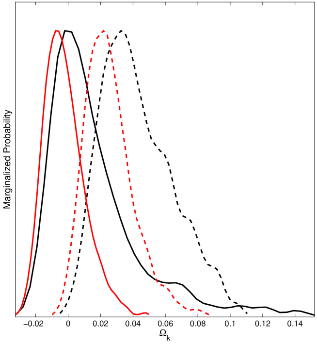
Figure 2: The marginalized probabilities of $\Omega_{k}$. The solid lines denote the results with $H_{0}=65$. The dashed lines denote the results with $H_{0}=72$. The black lines are for the dark energy model $w_{0}+w_{a}z/(1+z)^{2}$ and the red lines are for the model $w_{0}+w_{a}z/(1+z)$.

Since the angular scale of the sound horizon depends on the early history of the Universe, so it strongly depends on $\Omega_{r}$. However, we can neglect the effect of $\Omega_{r}$ when we evaluate the distance modules $\mu(z)$ and the shift parameter $R$ because the Universe is matter dominated. So only when we implement the CMB data with $l_{a}$, we need to consider the effect of $\Omega_{r}$. We know the energy density $\rho_{r}$ of radiation, so the dependence of $\Omega_{r}=8\pi G\rho_{r}/(3H_{0}^{2})$ is manifested by the Hubble constant $H_{0}$. Since we can neglect the effect of $\Omega_{r}$ in fitting SN Ia data, so the effect of the observed value of $H_{0}$ can be neglected by marginalizing over it. Therefore, we use the Hubble constant $H_{0}$ as a free parameter instead of $\Omega_{r}$. The marginalized probabilities of $\Omega_{k}$ for $H_{0}=65$ km/s/Mpc and $H_{0}=72$ km/s/Mpc are shown in Fig. 2. We see that the results indeed depend on $H_{0}$. As discussed in (Elgarøy & Multamäki, 2007), the combination of $R$ and $l_{a}$ approximates the WMAP3 data and the WMAP3 data depends on $H_{0}$ through $l_{a}$. So, as expected, $l_{a}$ also depends on $H_{0}$. From now on we also take $H_{0}$ as a fitting parameter, and impose a prior of $H_{0}=72\pm 8$ km/s/Mpc (Freedman, 2001). To understand why we can marginalize over $H_{0}$ in fitting SN Ia data and treat $H_{0}$ as a parameter in fitting WMAP3 data, we should think that we actually treat $\Omega_{r}$, not $H_{0}$ as a parameter when fitting the WMAP3 data. The parameter $H_{0}$ is not the observed Hubble constant when fitting the SN data because the normalization of the distance modulus was chosen arbitrarily. In summary, we have six fitting parameters for the DE models (8) and (10).

3 Results

In this section, we present our results. We first use the 182 gold SN Ia data (Riess et al., 2006), then we use the ESSENCE data (Riess et al., 2006; Wood-Vasey et al., 2007; Davis et al., 2007). For the SN Ia data, we consider both the SN Ia flux averaging with marginalization over $H_{0}$ (Wang, 2000; Wang & Mukherjee, 2004; Wang & Tegmark, 2004) and the analytical marginalization without the flux averaging. The results with the analytical marginalization are shown in solid lines and the results with flux averaging are shown in dashed lines. We also put the $\Lambda$CDM model with the symbol + in the contour plot.

3.1 Gold SN Ia data

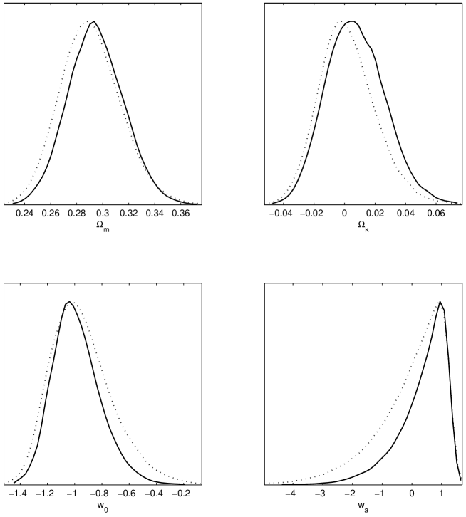
Figure 3: The marginalized probabilities for the DE model $w_{0}+w_{a}z/(1+z)$ by using the gold SN Ia data. The solid lines denote the results with analytical marginalization and the dashed lines denote the results with flux averaging.

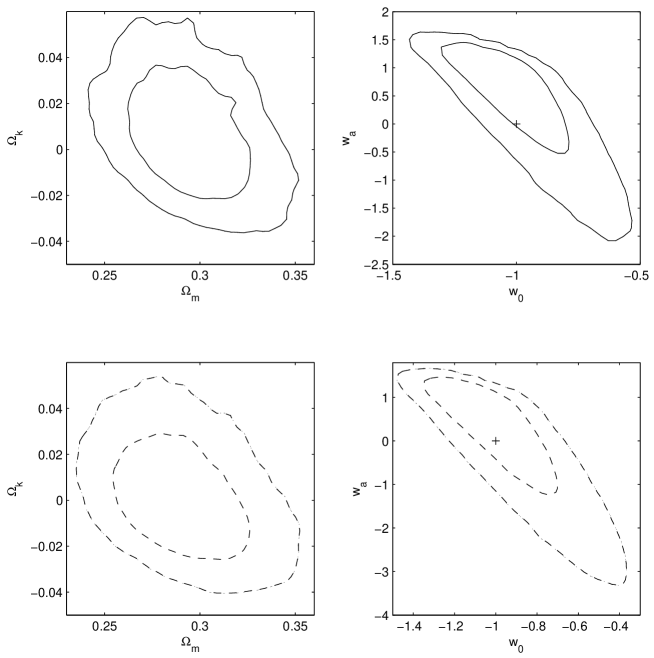
Figure 4: The marginalized $1\sigma$ and $2\sigma$ $\Omega_{m}$-$\Omega_{k}$ and $w_{0}$-$w_{a}$ contours for the DE model $w_{0}+w_{a}z/(1+z)$ by using the gold SN Ia data. The upper panels denote the results with analytical marginalization and the lower panels denote the results with flux averaging.

Fig. 3 shows the marginalized probabilities for $\Omega_{m}$, $\Omega_{k}$, $w_{0}$ and $w_{a}$ for the DE model $w_{0}+w_{a}z/(1+z)$. Fig. 4 shows the marginalized $\Omega_{m}$-$\Omega_{k}$ and $w_{0}$-$w_{a}$ contours. The $w_{0}$-$w_{a}$ contour with the flux averaging is consistent with the result in Wang & Mukherjee (2007). From Figs. 3 and 4, we see that the difference in the results between the analytical marginalization and the flux averaging is small. The $\Lambda$CDM model is consistent with the observation at the $1\sigma$ level. The value of $w_{a}$ is better constrained with the analytical marginalization.

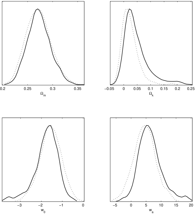
Figure 5: The marginalized probabilities for the DE model $w_{0}+w_{a}z/(1+z)^{2}$ by using the gold SN Ia data. The solid lines denote the results with analytical marginalization and the dashed lines denote the results with flux averaging.

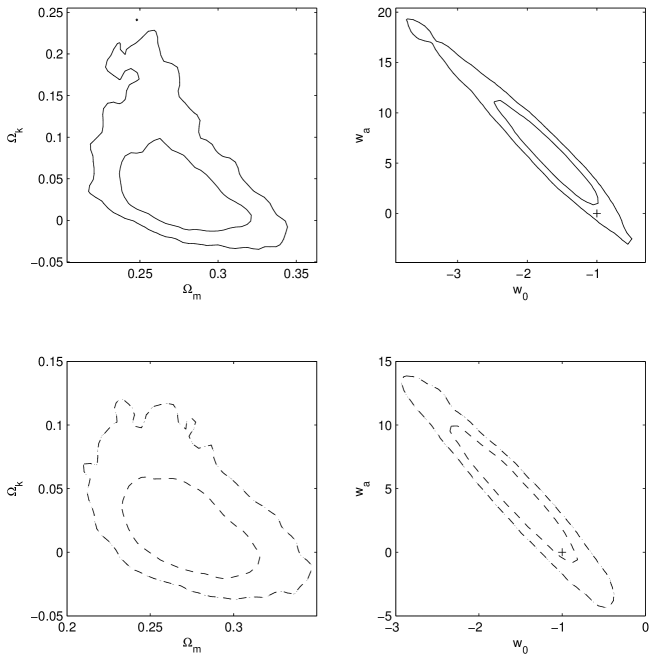
Figure 6: The marginalized $1\sigma$ and $2\sigma$ $\Omega_{m}$-$\Omega_{k}$ and $w_{0}$-$w_{a}$ contours for the DE model $w_{0}+w_{a}z/(1+z)^{2}$ by using the gold SN Ia data. The upper panels denote the results with analytical marginalization and the lower panels denote the results with flux averaging.

Fig. 5 shows the marginalized probabilities for $\Omega_{m}$, $\Omega_{k}$, $w_{0}$ and $w_{a}$ for the DE model $w_{0}+w_{a}z/(1+z)^{2}$. Fig. 6 shows the marginalized $\Omega_{m}$-$\Omega_{k}$ and $w_{0}$-$w_{a}$ contours. From Figs. 5 and 6, we see that the parameters are a little better constrained with the flux averaging. For the analytical marginalization, the $\Lambda$CDM model is consistent with the observation at the $2\sigma$ level. For the flux averaging, the $\Lambda$CDM model is consistent with the observation at the $1\sigma$ level.

3.2 ESSENCE data

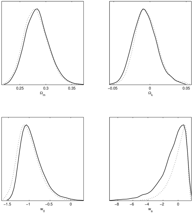
Figure 7: The marginalized probability distributions for the dark energy model $w_{0}+w_{a}z/(1+z)$ by using the ESSENCE data. The solid lines denote the results without flux average and the dashed lines denote the results with flux average.

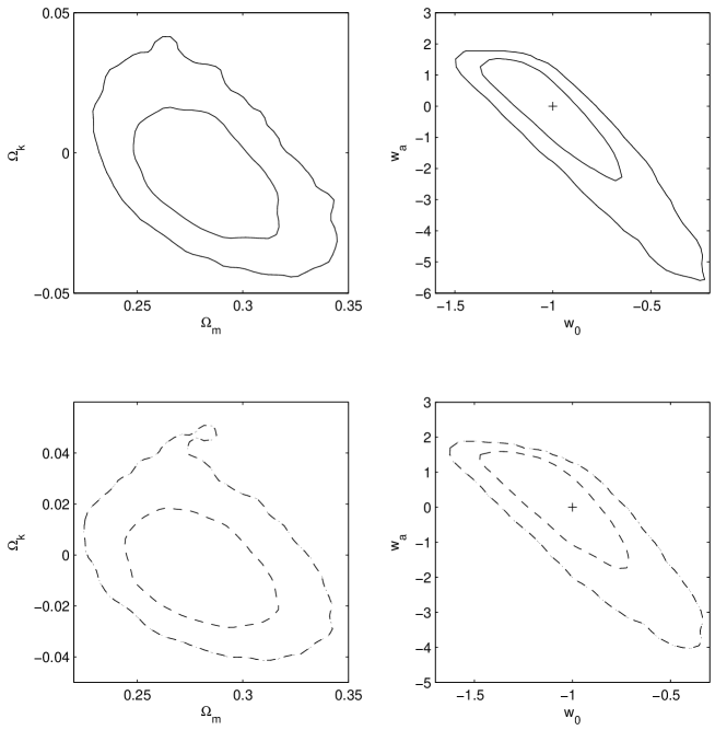
Figure 8: The marginalized $\Omega_{m}$-$\Omega_{k}$ and $w_{0}$-$w_{a}$ contours for the dark energy model $w_{0}+w_{a}z/(1+z)$ by using the ESSENCE data. The upper panels denote the results without flux average and the lower panels denote the results with flux average.

Fig. 7 shows the marginalized probabilities for $\Omega_{m}$, $\Omega_{k}$, $w_{0}$ and $w_{a}$ for the DE model $w_{0}+w_{a}z/(1+z)$. Fig. 8 shows the marginalized $\Omega_{m}$-$\Omega_{k}$ and $w_{0}$-$w_{a}$ contours. From Figs. 7 and 8, we see that the difference in the results between the analytical marginalization and the flux averaging is small. The $\Lambda$CDM model is consistent with the observation at the $1\sigma$ level.

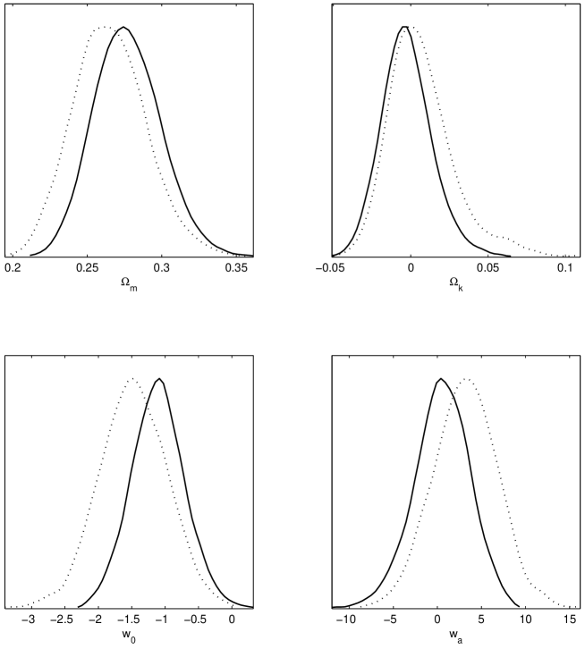
Figure 9: The marginalized probability distributions for the dark energy model $w_{0}+w_{a}z/(1+z)^{2}$ by using the ESSENCE data. The solid lines denote the results without flux average and the dashed lines denote the results with flux average.

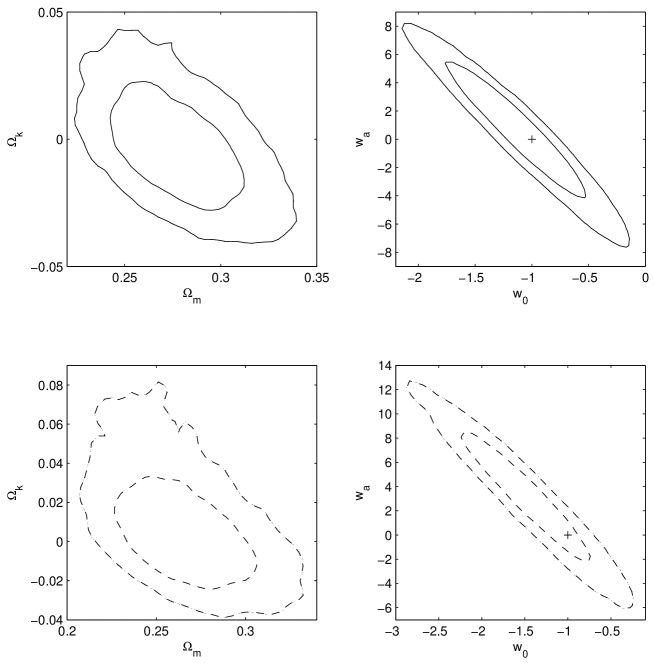
Figure 10: The marginalized $\Omega_{m}$-$\Omega_{k}$ and $w_{0}$-$w_{a}$ contours for the dark energy model $w_{0}+w_{a}z/(1+z)^{2}$ by using the ESSENCE data. The upper panels denote the results without flux average and the lower panels denote the results with flux average.

Fig. 9 shows the marginalized probabilities for $\Omega_{m}$, $\Omega_{k}$, $w_{0}$ and $w_{a}$ for the DE model $w_{0}+w_{a}z/(1+z)^{2}$. Fig. 10 shows the marginalized $\Omega_{m}$-$\Omega_{k}$ and $w_{0}$-$w_{a}$ contours. From Figs. 9 and 10, we see that the parameters are a little better constrained with the analytical marginalization. The $\Lambda$CDM model is consistent with the observation at the $1\sigma$ level.

We summarize the results in Tables 1 and 2. We do not see much improvement on the constraints on the DE parameters and the cosmic curvature by using the flux averaging method. For the DE model $w_{0}+w_{a}z/(1+z)$, the gold data gives better constraints than the ESSENCE data on the DE parameters $w_{0}$ and $w_{a}$, but both data give good constraints on the cosmic curvature. For the DE model $w_{0}+w_{a}z/(1+z)^{2}$, the ESSENCE data gives much better constraint on the cosmic curvature than the gold data, although the constraints on the DE parameters $w_{0}$ and $w_{a}$ are almost the same for both data. For the 182 gold data, the DE model $w_{0}+w_{a}z/(1+z)$ gives much better constraints on the cosmic curvature $\Omega_{k}$. For the ESSENCE data, the two DE models give almost the same constraint on $\Omega_{m}$ and $\Omega_{k}$. For the DE model $w_{0}+w_{a}z/(1+z)$, the mean value of $w_{0}$ determined from the observation tends to be $w_{0}\geq-1$, while the mean value of $w_{0}$ is less than $-1$ for the DE model $w_{0}+w_{a}z/(1+z)^{2}$.

From Tables 1 and 2, we see that the constraints on $\Omega_{k}$ are almost the same for the two different DE models (8) and (10). In other words, the results we obtained on $\Omega_{k}$ do not depend on the chosen models much. Recently, the authors in Clarkson et al. (2007) found that the assumption of a flat universe induces critically large errors in reconstructing the dark energy equation of state at $z\gtrsim 0.9$ even if the true cosmic curvature is very small, $\Omega_{k}\sim 0.01$ or less. They obtained the result by fitting the data derived from a DE model with $\Omega_{k}\neq 0$ with a flat model, so the result may not be conclusive. To see how the value of $\Omega_{k}$ affect the constraints on the property of DE, we perform the MCMC analysis on the DE models (8) and (10) with $\Omega_{k}=0$. The results are reported in Tables 3 and 4. Although the uncertainties of $\Omega_{k}$ change the values of $w_{0}$ and $w_{a}$, the ranges of $w_{0}$ and $w_{a}$ are almost the same for small $\Omega_{k}$.

In conclusion, we first confirm previous results that the shift parameter $R$ alone does not give good constraint on $\Omega_{k}$, we must combine $R$ and $l_{a}$ to constrain $\Omega_{k}$. By using $R$, $l_{a}$ and their covariance matrix, we get almost the same results as those obtained by using the original WMAP3 data. Without calculating the power spectrum, the fitting process is much faster and efficient. The cosmic curvature is found to be $|\Omega_{k}|\lesssim 0.03$.

Appendix A Analytical marginalization on $H_{0}$

By assuming a flat prior $P(H_{0})=1$ for $H_{0}$, the marginalization over $H_{0}$ means

$$L=e^{-\chi^{2}_{m}/2}=\int e^{-\chi^{2}/2}P(H_{0})dH_{0}=\int e^{-\chi^{2}/2}dH_{0}.$$ (A1)

Let $x=5\log_{10}H_{0}$ and $\alpha_{i}=\mu_{obs}(z_{i})-25-5\log_{10}[(1+z_{i}){\rm sinn}(\sqrt{|\Omega_{k}|}\int_{0}^{z_{i}}dz^{\prime}/E(z^{\prime}))/\sqrt{|\Omega_{k}|}]$, and substitute Eq. (1) into the above Eq. (A1), we get

$$\begin{array}[]{cl}L&=\frac{\ln 10}{5}\int dx\exp\left[-\frac{1}{2}\sum_{i}\frac{(\alpha_{i}+x)^{2}}{\sigma^{2}_{i}}+\frac{\ln 10}{5}x\right]\\ &=\frac{\ln 10}{5}\int dx\exp\left[-\frac{1}{2}\left(\sum_{i}\frac{1}{\sigma_{i}^{2}}\right)\left(x+\frac{\sum_{i}\alpha_{i}/\sigma_{i}^{2}-\ln 10/5}{\sum_{i}1/\sigma_{i}^{2}}\right)^{2}\right.\\ &\left.\ \ \ -\frac{1}{2}\sum_{i}\frac{\alpha^{2}_{i}}{\sigma^{2}_{i}}+\frac{1}{2}\frac{(\sum_{i}\alpha_{i}/\sigma_{i}^{2}-\ln 10/5)^{2}}{\sum_{i}1/\sigma_{i}^{2}}\right]\\ &=\frac{\ln 10}{5}\left(\frac{2\pi}{\sum_{i}1/\sigma_{i}^{2}}\right)^{1/2}\exp(-\frac{1}{2}\sum_{i}\frac{\alpha^{2}_{i}}{\sigma^{2}_{i}}+\frac{1}{2}\frac{(\sum_{i}\alpha_{i}/\sigma_{i}^{2}-\ln 10/5)^{2}}{\sum_{i}1/\sigma_{i}^{2}}).\end{array}$$ (A6)

So the minimum $\chi^{2}$ is

$$\chi^{2}_{m}=\sum_{i}\frac{\alpha^{2}_{i}}{\sigma^{2}_{i}}-\frac{(\sum_{i}\alpha_{i}/\sigma_{i}^{2}-\ln 10/5)^{2}}{\sum_{i}1/\sigma_{i}^{2}}-2\ln\left(\frac{\ln 10}{5}\sqrt{\frac{2\pi}{\sum_{i}1/\sigma_{i}^{2}}}\right).$$ (A7)

Table 1: The marginalized results with $1\sigma$ errors for the model $w_{0}+w_{a}z/(1+z)$

	Gold Data		Essence Data
	Analytical	Flux	Analytical	Flux
$\Omega_{m}$	$0.29^{+0.03}_{-0.02}$	$0.29\pm 0.02$	$0.28^{+0.03}_{-0.02}$	$0.28\pm 0.02$
$\Omega_{k}$	$0.007^{+0.023}_{-0.019}$	$0.002\pm 0.018$	$-0.007\pm 0.016$	$-0.004^{+0.015}_{-0.016}$
$w_{0}$	$-0.99^{+0.18}_{-0.16}$	$-0.95\pm 0.22$	$-0.94\pm 0.25$	$-1.0^{+0.24}_{-0.26}$
$w_{a}$	$0.34\pm 0.77$	$-0.05^{+1.04}_{-1.09}$	$-0.70^{+1.54}_{-1.52}$	$-0.26^{+1.29}_{-1.31}$

Table 2: The marginalized results with $1\sigma$ errors for the model $w_{0}+w_{a}z/(1+z)^{2}$

	Gold Data		Essence Data
	Analytical	Flux	Analytical	Flux
$\Omega_{m}$	$0.27^{+0.03}_{-0.02}$	$0.27^{+0.03}_{-0.02}$	$0.28^{+0.02}_{-0.03}$	$0.29\pm 0.02$
$\Omega_{k}$	$0.05\pm 0.04$	$0.02^{+0.03}_{-0.02}$	$-0.002^{+0.015}_{-0.016}$	$-0.013\pm 0.011$
$w_{0}$	$-1.8^{+0.6}_{-0.5}$	$-1.6^{+0.6}_{-0.5}$	$-1.1\pm 0.4$	$-1.1^{+0.4}_{-0.5}$
$w_{a}$	$6.4\pm 3.6$	$4.5\pm 3.6$	$0.5\pm 3.1$	$0.6\pm 3.3$

Table 3: The marginalized results with $1\sigma$ errors for the model $w_{0}+w_{a}z/(1+z)$ with $\Omega_{k}=0$

	Gold Data		Essence Data
	Analytical	Flux	Analytical	Flux
$\Omega_{m}$	$0.29\pm 0.02$	$0.29\pm 0.02$	$0.27^{+0.02}_{-0.01}$	$0.27\pm 0.02$
$w_{0}$	$-0.98^{+0.17}_{-0.13}$	$-0.98\pm 0.20$	$-1.06^{+0.18}_{-0.17}$	$-1.09\pm 0.22$
$w_{a}$	$0.28^{+0.65}_{-0.64}$	$0.15\pm 0.78$	$0.17^{+0.79}_{-0.85}$	$0.28\pm 0.87$

Table 4: The marginalized results with $1\sigma$ errors for the model $w_{0}+w_{a}z/(1+z)^{2}$ with $\Omega_{k}=0$

	Gold Data		Essence Data
	Analytical	Flux	Analytical	Flux
$\Omega_{m}$	$0.29\pm 0.02$	$0.28\pm 0.02$	$0.27\pm 0.02$	$0.27\pm 0.02$
$w_{0}$	$-1.23\pm 0.26$	$-1.22^{+0.31}_{-0.30}$	$-1.15^{+0.29}_{-0.30}$	$-1.29^{+0.33}_{-0.32}$
$w_{a}$	$2.28^{+1.75}_{-1.71}$	$1.94^{+1.98}_{-1.96}$	$1.01^{+2.15}_{-2.14}$	$1.87^{+2.11}_{-2.12}$

References

• Alam et al. (2004a) Alam, U., Sahni, V., Saini, T.D. & Starobinsky, A. A. 2004a, MNRAS, 354, 275
• Alam et al. (2004b) Alam, U., Sahni, V., & Starobinsky, A. A. 2004b, J. Cosmol. Astropart. Phys., JCAP 0406(2004)008
• Astier (2001) Astier, P. 2001, Phys. Lett. B, 500, 8
• Barger et al. (2007) Barger, V., Gao,Y. & Marfatia, D. 2007, Phys. Lett. B, 648, 127
• Cardone et al. (2004) Cardone, V. F., Troisi, A. & Capozziello, S. 2004, Phys. Rev. D, 69, 083517
• Chevallier & D. Polarski (2001) Chevallier, M. & Polarski, D. 2001, Int. J. Mod. Phys. D, 10, 213
• Choudhury & Padmanabhan (2005) Choudhury, T. R. & Padmanabhan, T. 2005, Γ₯, 429, 807
• Clarkson et al. (2007) Clarkson, C., Cortes, M. & Bassett, B. A. 2007, JCAP, 0708, 011.
• Copeland et al. (2006) Copeland, E. J., Sami, M. & Tsujikawa, S. 2006, Int. J. Mod. Phys. D, 15, 1753
• Corasaniti & Copeland (2003) Corasaniti, P.S. & Copeland, E. J. 2003, Phys. Rev. D, 67, 063521
• Davis et al. (2007) Davis, T.M. et al., 2007, arXiv: astro-ph/0701510.
• Efstathiou (1999) Efstathiou, G. 1999, MNRAS, 310, 842
• Eisenstein et al. (2005) Eisenstein, D. J. et al., 2005, ApJ, 633, 560
• ElgarΓΈy & MultamΓ€ki (2007) ElgarΓΈy, O. & MultamΓ€ki, T. 2007, arXiv: astro-ph/0702343
• Freedman (2001) Freedman, W. L. et al., 2001, ApJ, 553, 47
• Gerke & Efstathiou (2002) Gerke, B. F. & Efstathiou, G. 2002, MNRAS, 335, 33
• Gong (2005a) Gong, Y. G. 2005a, Int. J. Mod. Phys. D, 14, 599
• Gong (2005b) Gong, Y. G. 2005b, Class. Quantum Grav., 22, 2121
• Gong & Zhang (2005) Gong, Y. G. & Zhang, Y. Z. 2005, Phys. Rev. D, 72, 043518
• Gong & Wang (2006) Gong, Y. G. & Wang, A. 2006, Phys. Rev. D, 73, 083506
• Gong & Wang (2007a) Gong, Y. G. & Wang, A. 2007a, Phys. Rev. D, 75, 043520
• Gong & Wang (2007b) Gong, Y.G. & Wang, A. 2007b, Phys. Lett. B, 652, 63
• Gong et al. (2007) Gong, Y. G., Wang, A., Wu, Q. & Zhang, Y. Z. 2007, astro-ph/0703583, JCAP in press
• Gu & Khlopov (2007) Gu, Y. Q. & Khlopov, M. Y. 2007, gr-qc/0701050
• Huterer & Turner (2001) Huterer, D. & Turner, M. S. 2001, Phys. Rev. D, 64, 123527
• Huterer & Cooray (2005) Huterer, D. & Cooray, A. 2005, Phys. Rev. D, 71, 023506
• Ichikawa et al. (2006) Ichikawa, K., Kawasaki, M., Sekiguchi, T. & Takahashi, T. 2006, J. Cosmol. Astropart. Phys., JCAP12(2006)005
• Ichikawa & Takahashi (2006) Ichikawa, K. & Takahashi, T. 2006, Phys. Rev. D, 73, 083526
• Ichikawa & Takahashi (2007) Ichikawa, K. & Takahashi, T. 2007, J. Cosmol. Astropart. Phys., JCAP02(2007)001
• Jassal et al. (2005) Jassal, H. K., Bagla, J. S. & Padmanabhan, T. 2005, MNRAS, 356, L11
• JΓΆnsson et al. (2004) JΓΆnsson, J., Goobar, A., Amanullah, R. & BergstrΓΆm, L. 2004, J. Cosmol. Astropart. Phys., JCAP 0409(2004)007
• Lee (2005) Lee, S. 2005, Phys. Rev. D, 71, 123528
• Lewis & Bridle (2002) Lewis, A. & Bridle, S. 2002, Phys. Rev. D, 66, 103511
• Linder (2003) Linder, E. V. 2003, Phys. Rev. Lett., 90, 091301
• Padmanabhan (2003) Padmanabhan, T. 2003, Phys. Rep., 380, 235
• Peebles & Ratra (2003) Peebles, P. J. E. & Ratra, B. 2003, Rev. Mod. Phys., 75, 559
• Perlmutter et al. (1999) Perlmutter, S. et al., 1999, ApJ, 517, 565
• Riess et al. (1998) Riess, A. G. et al., 1998, AJ, 116, 1009
• Riess et al. (2006) Riess, A. G. et al., 2006, arXiv: astro-ph/0611572
• Sahni & Starobinsky (2000) Sahni, V. & Starobinsky, A. A., 2000, Int. J. Mod. Phys. D, 9, 373
• Sahni (2005) Sahni, V. 2005, The Physics of the Early Universe, E. Papantonopoulos, Springer: New York, 141
• Setare et al. (2007) Setare, M. R., Zhang, J., & Zhang, X. 2007, J. Cosmol. Astropart. Phys., JCAP 0703(2007)007
• Spergel et al. (2007) Spergel, D. N. et al., 2007, ApJS, 170, 377
• Sullivan et al. (2007) Sullivan, S., Cooray, A. & Holz, D. E. 2007, arXiv: 0706.3730
• Wang (2000) Wang, Y. 2000, ApJ, 536, 531
• Wang & Mukherjee (2004) Wang, Y. & Mukherjee, P. 2004, ApJ, 606, 654
• Wang & Mukherjee (2006) Wang, Y. & Mukherjee, P. 2006, ApJ, 650, 1
• Wang & Mukherjee (2007) Wang, Y. & Mukherjee, P. 2007, arXiv: astro-ph/0703780
• Wang & Tegmark (2004) Wang, Y. & Tegmark, M. 2004, Phys. Rev. Lett., 92, 241302
• Weller & Albrecht (2001) Weller, J. & Albrecht, A. 2001, Phys. Rev. Lett., 86, 1939
• Weller & Albrecht (2002) Weller, J. & Albrecht, A. 2002, Phys. Rev. D, 65, 103512
• Wetterich (2004) Wetterich, C. 2004, Phys. Lett. B, 594, 17
• Wood-Vasey et al. (2007) Wood-Vasey, W. M. et al., 2007, arXiv: astro-ph/0701041
• Zhu et al. (2004) Zhu, Z. H., Fujimoto, M. K. & He, X. T. 2004, Γ₯, 417, 833
Refer to caption