Erasmo Recami

Facoltà di Ingegneria, Università statale di Bergamo, Bergamo, Italy;

and INFN—Sezione di Milano, Milan, Italy.

Michel Zamboni-Rached,

Centro de Ciências Naturais e Humanas, Universidade Federal do ABC, Santo André, SP, Brasil

and

H. E. Hernández-Figueroa

DMO–FEEC, State University at Campinas, Campinas, SP, Brazil.

Abstract  –  In the first part of this paper (mainly a review) we present general and formal (simple) introductions to the ordinary gaussian waves and to the Bessel waves, by explicitly separating the cases of the beams from the cases of the pulses; and, finally, an analogous introduction is presented for the Localized Waves (LW), pulses or beams. Always we stress the very different characteristics of the gaussian with respect to the Bessel waves and to the LWs, showing the numerous and important properties of the latter w.r.t. the former ones: Properties that may find application in all fields in which an essential role is played by a wave-equation (like electromagnetism, optics, acoustics, seismology, geophysics, gravitation, elementary particle physics, etc.).       In the second part of this paper (namely, in its Appendix) we recall at first how, in the seventies and eighties, the geometrical methods of Special Relativity (SR) predicted —in the sense below specified— the existence of the most interesting LWs, i.e., of the X-shaped pulses. At last, in connection with the circumstance that the X-shaped waves are endowed with Superluminal group-velocities (as carefully discussed in the first part of this article), we briefly mention the various experimental sectors of physics in which Superluminal motions seem to appear: In particular, a bird’s-eye view is presented of the experiments till now performed with evanescent waves (and/or tunneling photons), and with the “localized Superluminal solutions” to the wave equations.

1 A GENERAL INTRODUCTION

1.1 Preliminary remarks

Diffraction and dispersion are known since long to be phenomena limiting the applications of (optical, for instance) beams or pulses.

Diffraction is always present, affecting any waves that propagate in two or three-dimensional media, even when homogeneous. Pulses and beams are constituted by waves traveling along different directions, which produces a gradual spatial broadening[6]. This effect is really a limiting factor whenever a pulse is needed which maintains its transverse localization, like, e.g., in free space communications[7], image forming[8], optical lithography[9, 10], electromagnetic tweezers[11, 12], etcetera.

Dispersion acts on pulses propagating in material media, causing mainly a temporal broadening: An effect known to be due to the variation of the refraction index with the frequency, so that each spectral component of the pulse possesses a different phase-velocity. This entails a gradual temporal widening, which constitutes a limiting factor when a pulse is needed which maintains its time width, like, e.g., in communication systems[13].

It is important, therefore, to develop any techniques able to reduce those phenomena.  The so-called localized waves (LW), known also as non-diffracting waves, are indeed able to resist diffraction for a long distance in free space.  Such solutions to the wave equations (and, in particular, to the Maxwell equations, under weak hypotheses) were theoretically predicted long time ago[14, 15, 16, 17] (cf. also[18], and the Appendix of this paper), mathematically constructed in more recent times[19, 20], and soon after experimentally produced[21, 22, 23].  Today, localized waves are well-established both theoretically and experimentally, and are having innovative applications not only in vacuum, but also in material (linear or non-linear) media, showing to be able to resist also dispersion.  As we were mentioning, their potential applications are being intensively explored, always with surprising results, in fields like Acoustics, Microwaves, Optics, and are promising also in Mechanics, Geophysics, and even Gravitational Waves and Elementary particle physics.  Worth noticing appear also the applications of the so-called “Frozen Waves”, that will be presented elsewhere in this book; while rather interesting are the applications already obtained, for instance, in high-resolution ultra-sound scanning of moving organs in human body[24, 25].

To confine ourselves to electromagnetism, let us recall the present-day studies on electromagnetic tweezers[26, 27, 28, 29], optical (or acoustic) scalpels, optical guiding of atoms or (charged or neutral) corpuscles[30, 31, 32], optical litography[33, 26], optical (or acoustic) images[34], communications in free space[35, 36, 19, 37], remote optical alignment[38], optical acceleration of charged corpuscles, and so on.

In the following two Subsections we are going to set forth a brief introduction to the theory and applications of localized beams and localized pulses, respectively.

Localized (non-diffracting) beams — The word beam refers to a monochromatic solution to the considered wave equation, with a transverse localization of its field. To fix our ideas, we shall explicitly refer to the optical case: But our considerations, of course, hold for any wave equation (vectorial, spinorial, scalar…: in particular, for the acoustic case too).

The most common type of optical beam is the gaussian one, whose transverse behavior is described by a gaussian function. But all the common beams suffer a diffraction, which spoils the transverse shape of their field, widening it gradually during propagation. As an example, the transverse width of a gaussian beam doubles when it travels a distance $z_{\rm dif}=\sqrt{3}\pi\Delta\rho_{0}^{2}/\lambda_{0}$, where $\Delta\rho_{0}$ is the beam initial width and $\lambda_{0}$ is its wavelength. One can verify that a gaussian beam with an initial transverse aperture of the order of its wavelength will already double its width after having travelled along a few wavelenths.

It was generally believed that the only wave devoid of diffraction was the plane wave, which does not suffer any transverse changes. Some authors had shown, actually, that it isn’t the only one. For instance, in 1941 Stratton[15] obtained a monochromatic solution to the wave equation whose transverse shape was concentrated in the vicinity of its propagation axis and represented by a Bessel function. Such a solution, now called a Bessel beam, was not subject to diffraction, since no change in its transverse shape took place with time. In ref.[16] it was later on demonstrated how a large class of equations (including the wave equations) admit “non-distorted progressing waves” as solutions; while already in 1915, in ref.[17], and subsequently in articles like ref.[39], it was shown the existence of soliton-like, wavelet-type solutions to the Maxwell equations. But all such literature did not raise the attention it deserved. In the case of ref.[15], this can be partially justified since that (Bessel) beam was endowed with infinite energy [as much as the plane waves]. An interesting problem, therefore, was that of investigating what it would happen to the ideal Bessel beam solution when truncated by a finite transverse aperture.

Only in 1987 a heuristical answer came from the known experiment by Durnin et al.[40], when it was shown that a realistic Bessel beam, endowed with wavelength $\lambda_{0}=0.6328\;\mu$m and central spot $\Delta\rho_{0}=59\;\mu$m, passing through an aperture with radius $R=3.5\;$mm is able to travel about $85\;$cm keeping its transverse intensity shape approximately unchanged (in the region $\rho<<R$ surrounding its central peak). In other words, it was experimentally shown that the transverse intensity peak, as well as the field in the surroundings of it, do not meet any appreciable change in shape all along a large “depth of field”. As a comparison, let us recall once more that a gaussian beam with the same wavelength, and with the central “spot” $\Delta\rho_{0}=59\;\mu$m, when passing through an aperture with the same radius $R=3.5\;$mm, doubles its transverse width after $3\;$cm, and after $6\;$cm its intensity is already diminished of a factor 10.  Therefore, in the considered case, a Bessel beams can travel, approximately without deformation, a distance 28 times larger than a gaussian beam’s.

Such a remarkable property is due to the fact that the transverse intensity fields (whose value decreases with increasing $\rho$), associated with the rings which constitute the (transverse) structure of the Bessel beam, when diffracting, end up reconstructing the beam itself, all along a large field-depth. All this depends on the Bessel beam spectrum (wavenumber and frequency),[34, 41, 38] as explained in detail in our ref.[42].  Let us stress that, given a Bessel and a gaussian beam —both with the same spot $\Delta\rho_{0}$ and passing through apertures with the same radius $R$ in the plane $z=0$, and with the same energy $E$— the percentage of the total energy $E$ contained inside the central peak region ($0\leq\rho\leq\Delta\rho_{0}$) is smaller for a Bessel than for a gaussian one: This different energy-distribution on the transverse plane is responsible for the reconstruction of the Bessel-beam central peak even at large distances from the source (and even after an obstacle with a size smaller than the aperture[71, 114, 78]: a nice property possessed also by the localized pulses we are going to examine below[114]).

It may be worth mentioning that most experiments carried on in this area have been performed rapidly and with use, often, of rather simple apparata: The Durnin et al.’s experiment, e.g., had recourse, for the generation of a Bessel beam, to a laser source, an annular slit and a lens, as depicted in Fig.(1). In a sense, such an apparatus produces what can be regarded as the cylindrically symmetric generalization of a couple of plane waves emitted at angles $theta$ and $-theta$, w.r.t. the $z$-direction, respectively (in which case the plane wave intersection moves along $z$ with the speed $c/\sin\theta$).  Of course, these non-diffracting beams can be generated also by a a conic lens (axicon) [cf., e.g., ref.[34]], or by other means like holographic elements [cf., e.g., refs.[38, 44]].

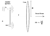
Figure 1: The simple experimental set-up used by Durnin et al. for generating a Bessel beam.

Let us emphasize, as already mentioned at the end of the previous Subsection, that nowadays a lot of interesting applications of non-diffracting beams are being investigated; besides the Lu et al.’s ones in Acoustics. In the optical sector, let us recall again those of using Bessel beams as optical tweezers able to confine or move around small particles.  In such theoretical and application areas, a noticeable contribution is the one presented in refs.[45, 46, 77], wherein, by suitable superpositions of Bessel beams endowed with the same frequency but different longitudinal wavenumbers, stationary fields have been mathematically constructed in closed form, which possess a high transverse localization and, more important, a longitudinal intensity-shape that can be freely chosen inside a predetermined space-interval $0\leq z\leq L$. For instance, a high intensity field, with a static envelope, can be created within a tiny region, with negligible intensity elsewhere: Chapter 2 of the coming book [Localized Waves (J.Wiley; in press] will deal, among the others, with such “Frozen Waves”.

Localized (non-diffracting) pulses — As we have seen in the previous Subsection, the existence of non-diffractive (or localized) pulses was predicted since long: cf., once more, refs.[17, 16], and, not less, refs.[14, 18], as well as more recent articles like refs.[47, 48].  The modern studies about non-diffractive pulses (to confine ourselves, at least, to the ones that attracted more attention) followed a development rather independent of those on non-diffracting beams, even if both phenomena are part of the same sector of physics: that of Localized Waves.

In 1983, Brittingham[49] set forth a luminal ($V=c$) solution to the wave equation (more particularly, to the Maxwell equations) with travels rigidly, i.e., without diffraction. The solution proposed in ref.[49] possessed however infinite energy, and once more the problem arose of overcoming such a problem.

A way out was first obtained, as far as we know, by Sezginer[50], who showed how to construct finite-energy luminal pulses, which —however— do not propagate without distortion for an infinite distance, but, as it is expected, travel with constant speed, and approximately without deforming, for a certain (long depth of field: much longer, in this case too, than that of the ordinary pulses like the gaussian ones. In a series of subsequent papers[35, 36, 51, 52, 53, 54], a simple theoretical method was developed, called by those authors “bidirectional decomposition”, for constructing a new series of non-diffracting, luminal pulses.

Eventually, at the beginning of the nineties, Lu et al.[19, 21] constructed, both mathematically and experimentally, new solutions to the wave equation in free space: namely, an X-shaped localized pulse, with the form predicted by the so-called extended Special Relativity[14, 1]; for the connection between what Lu et al. called “X-waves” and “extended” relativity see, e.g., ref.[18], while brief excerpts of that theory can be found, for instance, in refs.[55, 56, 20, 57, 58].  Lu et al.’s solutions were continuous superpositions of Bessel beams with the same phase-velocity (i.e., with the same axicon angle[59, 20, 19, 1], $alpha$): cf., e.g., Fig.(2); so that they could keep their shape for long distances.  Such X-shaped waves resulted to be interesting and flexible localized solutions, and have been afterwards studied in a number of papers, even if their velocity $V$ is supersonic or Superluminal ($V>c$): Actually, when the phase-velocity does not depend on the frequency, it is known that such a phase-velocity becomes the group-velocity!  Remembering how a superposition of Bessel beams is generated (for example, by a discrete or continuous set of annular slits or transducers), it results clear that the energy forming the X-waves, coming from those rings, travels at the ordinary speed $c$ of the plane waves in the considered medium[60, 61, 20, 62] [here $c$, representing the velocity of the plane waves in the medium, is the sound-speed in the acoustic case, and the speed of light in the electromagnetic case; and so on].  Nevertheless, the peak of the X-shaped waves is faster than $c$.

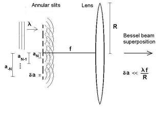
Figure 2: One of the simplest experimental set-ups for generating various kinds of Bessel beam superpositions.

It is possible to generate (besides the “classic” X-wave produced by Lu et al. in 1992) infinite sets of new X-shaped waves, with their energy more and more concentrated in a spot corresponding to the vertex region[42]. It may therefore appear rather intriguing that such a spot [even if no violations of special relativity (SR) is obviously implied: all the results come from Maxwell equations, or from the wave equations[73, 74]]— travels Superluminally when the waves are electromagnetic.  We shall call “Superluminal” all the X-shaped waves, even, e.g., when the waves are acoustic.  By Fig.(3), which refers to an X-wave possessing the velocity $V>c$, we illustrate the fact that, if its vertex or central spot is located at $P_{1}$ at time $t_{1}$, it will reach the position $P_{2}$ at a time $t+\tau$ where $\tau=|P_{2}-P_{1}|/V\;<\;|P_{2}-P_{1}|/c$:  We shall discuss all these points below.

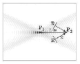
Figure 3: This figure shows an X-shaped wave, that is, a localized Superluminal pulse. It refers to an X-wave, possessing the velocity $V>c$, and illustrates the fact that, if its vertex or central spot is located at $P_{1}$ at time $t_{0}$, it will reach the position $P_{2}$ at a time $t+\tau$ where $\tau=|P_{2}-P_{1}|/V\;<\;|P_{2}-P_{1}|/c$: This is something different from the illusory “scissor effect”, even if the feeding energy, coming from the regions $R$, has travelled with the ordinary speed $c$ (which is the speed of light in the electromagnetic case, or the sound speed in Acoustics, and so on).

Soon after having mathematically and experimentally constructed their “classic” acoustic X-wave, Lu et al. started applying them to ultrasonic scanning, obtaining —as we already said— very high quality images.  Subsequently, in a 1996 e-print and report, Recami et al. (see, e.g., ref.[20] and refs. therein) published the analogous X-shaped solutions to the Maxwell equations: By constructing scalar Superluminal localized solutions for each component of the Hertz potential. That showed, by the way, that the localized solutions to the scalar equation can be used —under very weak conditions— for obtaining localized solutions to Maxwell’s equations too (actually, Ziolkowski et al.[43] had found something similar, called by them slingshot pulses, for the simple scalar case; but their solution had gone practically unnoticed).  In 1997 Saari et al.[22] announced, in an important paper, the production in the lab of an X-shaped wave in the optical realm, thus proving experimentally the existence of Superluminal electromagnetic pulses.  Three years later, in 2000, Mugnai et al.[23] produced, in an experiment of theirs, Superluminal X-shaped waves in the microwave region [their paper aroused various criticisms, to which those author however responded].

2 A MORE DETAILED INTRODUCTION

Let us refer[5] to the differential equation known as homogeneous wave equation: simple, but so important in Acoustics, Electromagnetism (Microwaves, Optics,…), Geophysics, and even, as we said, gravitational waves and elementary particle physics:

$$\left(\frac{\partial^{2}}{\partial x^{2}}+\frac{\partial^{2}}{\partial y^{2}}+\frac{\partial^{2}}{\partial z^{2}}-\frac{1}{c^{2}}\frac{\partial^{2}}{\partial t^{2}}\right)\,\psi(x,y,z;t)\;=\;0$$ (1)

Let us write it in the cylindrical co-ordinates $(\rho,\phi,z)$ and, for simplicity’s sake, confine ourselves to axially symmetric solutions $\psi(\rho,z;t)$.  Then, eq.(1) becomes

$$\left(\frac{\partial^{2}}{\partial\rho^{2}}+\frac{1}{\rho}\frac{\partial}{\partial\rho}+\frac{\partial^{2}}{\partial z^{2}}-\frac{1}{c^{2}}\frac{\partial^{2}}{\partial t^{2}}\right)\,\psi(\rho,z;t)\;=\;0\ .$$ (2)

In free space, solution $\psi(\rho,z;t)$ can be written in terms of a Bessel-Fourier transform w.r.t. the variable $\rho$, and two Fourier transforms w.r.t. variables $z$ and $t$, as follows:

$$\psi(\rho,z,t)\;=\;\int_{0}^{\infty}\int_{-\infty}^{\infty}\int_{-\infty}^{\infty}\,k_{\rho}\,J_{0}(k_{\rho}\,\rho)\,e^{ik_{z}z}\,e^{-i\omega t}\,\bar{\psi}(k_{\rho},k_{z},\omega)\,{\rm d}k_{\rho}\,{\rm d}k_{z}\,{\rm d}\omega$$ (3)

where $J_{0}(.)$ is an ordinary zero-order Bessel function and $\bar{\psi}(k_{\rho},k_{z},\omega)$ is the transform of $\psi(\rho,z,t)$.

Substituting eq.(3) into eq.(2), one obtains that the relation, among $\omega$, $k_{\rho}$ and $k_{z}\,$,

$$\frac{\omega^{2}}{c^{2}}\;=\;k_{\rho}^{2}+k_{z}^{2}$$ (4)

has to be satisfied.  In this way, by using condition (4) in eq.(3), any solution to the wave equation (2) can be written

$$\psi(\rho,z,t)\;=\;\displaystyle{\int_{0}^{\omega/c}\int_{-\infty}^{\infty}\,k_{\rho}\,J_{0}(k_{\rho}\,\rho)\,e^{i\sqrt{\omega^{2}/c^{2}\,-\,k_{\rho}^{2}}\,\,z}\,e^{-i\omega t}\,S(k_{\rho},\omega)\,{\rm d}k_{\rho}\,{\rm d}\omega}$$ (5)

where $S(k_{\rho},\omega)$ is the chosen spectral function.

The general integral solution (5) yields for instance the (non-localized) gaussian beams and pulses, to which we shall refer for illustrating the differences of the localized waves w.r.t. them.

The Gaussian Beam — A very common (non-localized) beam is the gaussian beam[76], corresponding to the spectrum

$$S(k_{\rho},\omega)\;=\;2a^{2}\,e^{-a^{2}k_{\rho}^{2}}\,\delta(\omega-\omega_{0})$$ (6)

In eq.(6), $a$ is a positive constant, which will be shown to depend on the transverse aperture of the initial pulse.

Figure 4 illustrates the interpretation of the integral solution (5), with spectral function (6), as a superposition of plane waves.  Namely, from Fig.4 one can easily realize that this case corresponds to plane waves propagating in all directions (always with $k_{z}\geq 0$), the most intense ones being those directed along (positive) $z$. Notice that in the plane-wave case $\vec{k_{z}}$ is the longitudinal component of the wave-vector, $\vec{k}=\vec{k_{\rho}}+\vec{k_{z}}$, where $\vec{k_{\rho}}=\vec{k_{x}}+\vec{k_{y}}$.

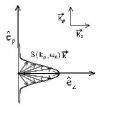
Figure 4: Visual interpretation of the integral solution (5), with the spectrum (6), in terms of a superposition of plane waves.

On substituting eq.(6) into eq.(5) and adopting the paraxial approximation, one meets the gaussian beam

$$\psi_{\rm gauss}(\rho,z,t)\;=\;\frac{\displaystyle{2a^{2}\,{\rm exp}\left(\displaystyle{\frac{-\rho^{2}}{4(a^{2}+i\,z/2k_{0})}}\right)}}{\displaystyle{2(a^{2}+i\,z/2k_{0})}}\,\,\displaystyle{e^{ik_{0}(z-ct)}}\;\;,$$ (7)

where $k_{0}=\omega_{0}/c$. We can verify that such a beam, which suffers transverse diffraction, doubles its initial width $\Delta\rho_{0}=2a$ after having traveled the distance $z_{{\rm dif}}\;=\;\sqrt{3}\,k_{0}\Delta\rho_{0}^{2}/2$, called diffraction length. The more concentrated a gaussian beam happens to be, the more rapidly it gets spoiled.

The Gaussian Pulse — The most common (non-localized) pulse is the gaussian pulse, which is got from eq.(5) by using the spectrum[75]

$$S(k_{\rho},\omega)\;=\;\frac{2ba^{2}}{\sqrt{\pi}}e^{-a^{2}k_{\rho}^{2}}e^{-b^{2}(\omega-\omega_{0})^{2}}$$ (8)

where $a$ and $b$ are positive constants. Indeed, such a pulse is a superposition of gaussian beams of different frequency.

Now, on substituting eq.(8) into eq.(5), and adopting once more the paraxial approximation, one gets the gaussian pulse:

$$\psi(\rho,z,t)\;=\;\frac{a^{2}\,{\rm exp}\left(\displaystyle{\frac{-\rho^{2}}{4(a^{2}+iz/2k_{0})}}\right){\rm exp}\left(\displaystyle{\frac{-(z-ct)^{2}}{4c^{2}b^{2})}}\right)}{a^{2}+iz/2k_{0}}\;\;,$$ (9)

endowed with speed $c$ and temporal width $\Delta t=2b$, and suffering a progressive enlargement of its transverse width, so that its initial value gets doubled already at position $z_{{\rm dif}}\;=\;\sqrt{3}\,k_{0}\Delta\rho_{0}^{2}/2\;$, with $\Delta\rho_{0}=2a$.

2.1 The localized solutions

Let us finally go on to the construction of the two most renowned localized waves: the Bessel beam, and the ordinary X-shaped pulse.[5]

First of all, it is interesting to observe that, when superposing (axially symmetrical) solutions of the wave equation in the vacuum, three spectral parameters come into the play, $(\omega,\ k_{\rho},\ k_{z})$, which have however to satisfy the constraint (4), deriving from the wave equation itself. Consequently, only two of them are independent: and we choose here $\omega$ and $k_{\rho}$.  Such a freedom in choosing $\omega$ and $k_{\rho}$ was already apparent in the spectral functions generating gaussian beams and pulses, which consisted in the product of two functions, one depending only on $\omega$ and the other on $k_{\rho}$.

We are going to see that particular relations between $\omega$ and $k_{\rho}$ [or, analogously, between $\omega$ and $k_{z}$] can be moreover imposed, in order to get interesting and unexpected results, such as the localized waves.

The Bessel beam — Let us start by imposing a linear coupling between $\omega$ and $k_{\rho}$ (it could be actually shown[41] that it is the unique coupling leading to localized solutions).

Namely, let us consider the spectral function

$$S(k_{\rho},\omega)\;=\;\frac{\delta(k_{\rho}-\displaystyle{\frac{\omega}{c}}\sin\theta)}{k_{\rho}}\,\,\delta(\omega-\omega_{0})\;\;,$$ (10)

which implies that $k_{\rho}=(\omega\sin\theta)/c$, with $0\leq\theta\leq\pi/2$: a relation that can be regarded as a space-time coupling. Let us add that this linear constraint between $\omega$ and $k_{\rho}$, together with relation (4), yields $k_{z}=(\omega\cos\theta)/c$. This is an important fact, since it has been shown elsewhere[42] that an ideal localized wave must contain a coupling of the type $\omega=Vk_{z}+b$, where $V$ and $b$ are arbitrary constants.

The interpretation of the integral function (5), this time with the spectrum (10), as a superposition of plane waves is visualized by Figure 5: which shows that an axially-symmetric Bessel beam is nothing but the result of the superposition of plane waves whose wave vectors lay on the surface of a cone having the propagation axis as its symmetry axis and an opening angle equal to $\theta$; such $\theta$ being called the axicon angle.

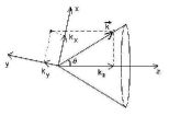
Figure 5: The axially-symmetric Bessel beam is created by the superposition of plane waves whose wave vectors lay on the surface of a cone having the propagation axis as its symmetry axis and angle equal to $\theta$ (”axicon angle”).

By inserting eq.(10) into eq.(5), one gets the mathematical expression of the so-called Bessel beam:

$$\psi(\rho,z,t)\;=\;J_{0}\left(\frac{\omega_{0}}{c}\sin\theta\,\,\rho\right)\,{\rm exp}\left[i\,\,\frac{\omega_{0}}{c}\cos\theta\,\left(z-\frac{c}{\cos\theta}t\right)\right]$$ (11)

This beam possesses phase-velocity $v_{\rm ph}=c/\cos\theta$, and field transverse shape represented by a Bessel function $J_{0}(.)$ so that its field in concentrated in the surroundings of the propagation axis $z$. Moreover, eq.(11) tells us that the Bessel beam keeps its transverse shape (which is therefore invariant) while propagating, with central “spot” $\Delta\rho=2.405c/(\omega\sin\theta)$.

The ideal Bessel beam, however, is not a square-integrable function, and possesses therefore an infinite energy, i.e., it cannot be experimentally produced.

But we can have recourse to truncated Bessel beams, generated by finite apertures. In this case the (truncated) Bessel beams are still able to travel a long distance while maintaining their transfer shape, as well as their speed, approximately unchanged[40, 69, 70]: That is to say, they still possess a large field-depth. For instance, the depth of field of a Bessel beam generated by a circular finite aperture with radius $R$ is given by

$$Z_{\rm max}\;=\;\frac{R}{\tan\theta}$$ (12)

where $\theta$ is the beam axicon angle. In the finite aperture case, the Bessel beam cannot be represented any longer by eq.(11), and one has to calculate it by the scalar diffraction theory: Using, for example, Kirchhoff’s or Rayleigh-Sommerfeld’s diffraction integrals. But until the distance $Z_{\rm max}$ one may still use eq.(11) for approximately describing the beam, at least in the vicinity of the axis $\rho=0$; namely, for $\rho<<R$. To realize how much a truncated Bessel beam succeeds in resisting diffraction, let us consider also a gaussian beam, with the same frequency and central “spot”, and compare their field-depths. In particular, let us assume for both beams $\lambda=0.63\,\mu$m and initial central “spot” size $\Delta\rho_{0}=60\,\mu$m. The Bessel beam will possess axicon angle $\theta=\arcsin(2.405c/(\omega\Delta\rho_{0}))=0.004\;$rad. Figure 6 depicts the behavior of the two beams for a Bessel beam circular aperture with radius $3.5\;$mm.  We can see how the gaussian beam doubles its initial transverse width already after $3\;$cm, and after $6\;$cm its intensity has become an order of magnitude smaller. By contrast, the truncated Bessel beam keeps its transverse shape untill the distance $Z_{\rm max}=R/\tan\theta=85\;$cm. Afterwards, the Bessel beam rapidly decays, as a consequence of the sharp cut performed on its aperture (such cut being responsible also for the intensity oscillations suffered by the beam along its propagation axis, and for the fact that eventually the feeding waves, coming from the aperture, at a certain point get faint).

Figure 6: Comparison between a gaussian (a) and a truncated Bessel beam (b). One can see that the gaussian beam doubles its initial transverse width already after $3\;$cm, while after $6\;$cm its intensity decays of a factor 10. By contrast, the Bessel beam does approximately keep its transverse shape till the distance $85\;$cm.

The zeroth-order (axially symmetric) Bessel beam is nothing but one example of localized beam. Further examples are the higher order (not cylindrically symmetric) Bessel beams

$$\psi(\rho,\phi,z;t)\;=\;J_{\nu}\left(\frac{\omega_{0}}{c}\sin\theta\,\,\rho\right)\,{\rm exp}(i\nu\phi)\;{\rm exp}\left(i\,\,\frac{\omega_{0}}{c}\cos\theta\,\left(z-\frac{c}{\cos\theta}t\right)\right)\;\;,$$ (13)

or the Mathieu beams[68], and so on.

The Ordinary X-shaped Pulse — Following the same procedure adopted in the previous subsection, let us construct pulses by using spectral functions of the type

$$S(k_{\rho},\omega)\;=\;\frac{\delta(k_{\rho}-\displaystyle{\frac{\omega}{c}}\sin\theta)}{k_{\rho}}\,\,F(\omega)$$ (14)

where this time the Dirac delta function furnishes the spectral space-time coupling $k_{\rho}=(\omega\sin\theta)/c$. Function $F(\omega)$ is, of course, the frequency spectrum; it is left for the moment undetermined.

On using eq.(14) into eq.(5), one obtains

$$\psi(\rho,z,t)\;=\;\int_{-\infty}^{\infty}\,F(\omega)\,J_{0}\left(\frac{\omega}{c}\sin\theta\,\,\rho\right)\,{\rm exp}\left(\frac{\omega}{c}\cos\theta\,\left(z-\frac{c}{\cos\theta}t\right)\right)\,{\rm d}\omega\ .$$ (15)

It is easy to see that $\psi$ will be a pulse of the type

$$\psi\;=\;\psi(\rho,z-Vt)$$ (16)

with a speed $V=c/\cos\theta$ independent of the frequency spectrum $F(\omega)$.

Such solutions are known as X-shaped pulses, and are localized (non-diffractive) waves in the sense that they maintain their spatial shape during propagation (see., e.g., refs.[19, 20, 42] and refs. therein).

At this point, some remarkable observations are in order:

(i) When a pulse consists in a superposition of waves (in this case, Bessel beams) all endowed with the same phase-velocity $V_{\rm ph}$ (in this case, with the same axicon angle) independent of their frequency, then it is known that the phase-velocity (in this case $V_{\rm ph}=c/\cos\theta$) becomes the group-velocity[72, 64] $V$: That is, $V=c/\cos\theta>c$. In this sense, the X-shaped waves are called “Superluminal localized pulses” (cf., e.g., ref.[20] and refs. therein).

(ii) Such pulses, even if their group-velocity is Superluminal, do not contradict standard physics, having been found in what precedes on the basis of the wave equations —in particular, of Maxwell equations[35, 20]— only. Indeed, as we shall better see in the historical Appendix, their existence can be understood within special relativity itself[14, 18, 20, 56, 55, 57], on the basis of its ordinary Postulates[1]. Actually, let us repeat it, they are fed by waves originating at the aperture and carrying energy with the standard speed $c$ of the medium (the light-velocity in the electromagnetic case, and the sound-velocity in the acoustic[21] case).  We can become convinced about the possibility of realizing Superluminal X-shaped pulses by imagining the simple ideal case of a negligibly sized Superluminal source $S$ endowed with speed $V>c$ in vacuum, and emitting electromagnetic waves $W$ (each one traveling with the invariant speed $c$). The electromagnetic waves will result to be internally tangent to an enveloping cone $C$ having $S$ as its vertex, and as its axis the propagation line $z$ of the source[1, 18]: This is completely analogous to what happens for an airplane that moves in air with constant supersonic speed.  The waves $W$ interfere mainly negatively inside the cone $C$, and constructively on its surface.  We can place a plane detector orthogonally to $z$, and record magnitude and direction of the $W$ waves that hit on it, as (cylindrically symmetric) functions of position and of time.  It will be enough, then, to replace the plane detector with a plane antenna which emits —instead of recording— exactly the same (axially symmetric) space-time pattern of waves $W$, for constructing a cone-shaped electromagnetic wave $C$ that will propagate with the Superluminal speed $V$ (of course, without a source any longer at its vertex):  even if each wave $W$ travels with the invariant speed $c$.  Once more, this is exactly what would happen in the case of a supersonic airplane (in which case $c$ is the sound speed in air: for simplicity, assume the observer to be at rest with respect to the air).  For further details, see the quoted references.  Actually, by suitable superpositions, and interference, of speed-$c$ waves, one can obtain pulses more and more localized in the vertex region[42]: That is, very localized field-“blobs” traveling with Superluminal group-velocity.  This has nothing to do with the illusory “scissors effect”, since such blobs, along their field-depth, are a priori able, e.g., to get two successive (weak) detectors, located at distance $L$, clicking after a time smaller than $L/c$. Incidentally, an analysis of the above-mentioned case (that of a supersonic plane or a Superluminal charge) led, as expected[1], to the simplest type of “X-shaped pulse”[18].  It might be useful, finally, to recall that SR (even the wave-equations have an internal relativistic structure!) implies considering also the forward cone: cf. Fig.7. The truncated X-waves considered in this paper, for instance, must have a leading cone in addition to the rear cone; such a leading cone having a role for the peak stability[19]: For example, in the approximate case in which we produce a finite conic wave truncated both in space and in time, the theory of SR suggested the bi-conic shape (symmetrical in space with respect to the vertex $S$) to be a better approximation to a rigidly traveling wave (so that SR suggests to have recourse to a dynamic antenna emitting a radiation cylindrically symmetrical in space and symmetric in time, for a better approximation to an “undistorted progressing wave”).

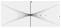
Figure 7: The truncated X-waves considered in this paper, as predicted by SR (all wave-equations have an intrinsic relativistic structure!), must have a leading cone in addition to the rear cone; such a leading cone having a role for the peak stability[19]: For example, when producing a finite conic wave truncated both in space and in time, the theory of SR suggested to have recourse, in the simplest case, to a dynamic antenna emitting a radiation cylindrically symmetrical in space and symmetric in time, for a better approximation to what Courant and Hilbert[16] called an “undistorted progressing wave”. See the following, in the text).

(iii) Any solutions that depend on $z$ and on $t$ only through the quantity $z-Vt$, like eq.(15), will appear the same to an observer traveling along $z$ with the speed $V$, whatever it be (subluminal, luminal or Superluminal) the value of $V$. That is, such a solution will propagate rigidly with speed $V$ (and in fact there exist Superluminal, luminal and subluminal localized waves). This further explains why our X-shaped pulses, after having been produced, will travel almost rigidly at speed $V$ (in this case, a faster-than-light group-velocity), all along their depth of field. To be even clearer, let us consider a generic function, depending on $z-Vt$ with $V>c$, and show, by explicit calculations involving the Maxwell equations only, that it obeys the scalar wave equation.  Following Franco Selleri[103], let us consider, e.g., the wave function

$$\Phi(x,y,z,t)\;=\;{\displaystyle{\frac{a}{{\sqrt{[b-ic(z-Vt)]^{2}+(V^{2}-c^{2})(x^{2}+y^{2})}}}}}$$ (17)

with $a$ and $b$ non-zero constants, $c$ the ordinary speed of light, and $V>c$  [incidentally, this wave function is nothing but the classic X-shaped wave in cartesian co-ordinates]. Let us naively verify that it is a solution to the wave equation

$$\mbox{\boldmath$\nabla$}^{2}\Phi(x,y,z,t)-{\frac{1}{c^{2}}}\;{\frac{\partial^{2}\Phi(x,y,z,t)}{\partial^{2}t}}\;=\;0\ .$$ (18)

On putting

$$R\,\equiv\,\displaystyle{{{\sqrt{[b-ic(z-Vt)]^{2}+(V^{2}-c^{2})(x^{2}+y^{2})}}}}\;,$$ (19)

one can write $\Phi=a/R$ and evaluate the second derivatives

$$\frac{1}{a}\,\frac{\partial^{2}\Phi}{\partial^{2}z}\;=\;\frac{c^{2}}{R^{3}}-\frac{3c^{2}}{R^{5}}\,[b-ic(z-Vt)]^{2}\ ;$$

$$\frac{1}{a}\,\frac{\partial^{2}\Phi}{\partial^{2}x}\;=\;-\frac{V^{2}-c^{2}}{R^{3}}\,+\,3\left(V^{2}-c^{2}\right)^{2}\;\frac{x^{2}}{R^{5}}\ ;$$

$$\frac{1}{a}\,\frac{\partial^{2}\Phi}{\partial^{2}y}\;=\;-\frac{V^{2}-c^{2}}{R^{3}}\,+\,3\left(V^{2}-c^{2}\right)^{2}\;\frac{y^{2}}{R^{5}}\;$$

$$\frac{1}{a}\,\frac{\partial^{2}\Phi}{\partial^{2}t}\;=\;\frac{c^{2}V^{2}}{R^{3}}-\frac{3c^{2}V^{2}}{R^{5}}\,[b-ic(z-Vt)]^{2}\ ;$$

wherefrom

$$\frac{1}{a}\,\left[\frac{\partial^{2}\Phi}{\partial^{2}z}-\frac{1}{c^{2}}\frac{\partial^{2}\Phi}{\partial^{2}t}\right]\;=\;-\frac{V^{2}-c^{2}}{R^{3}}+3\left(V^{2}-c^{2}\right)^{2}\;\frac{[b-ic(z-Vt)]^{2}}{R^{5}}\ ,$$

and

$$\frac{1}{a}\,\left[\frac{\partial^{2}\Phi}{\partial^{2}x}+\frac{\partial^{2}\Phi}{\partial^{2}y}\right]\;=\;-2\,\frac{V^{2}-c^{2}}{R^{3}}+3\left(V^{2}-c^{2}\right)^{2}\;\frac{x^{2}+y^{2}}{R^{5}}\ .$$

From the last two equations, remembering the previous definition, one finally gets

$$\frac{1}{a}\,\left[{\frac{\partial^{2}\Phi}{\partial^{2}z}}+{\frac{\partial^{2}\Phi}{\partial^{2}x}}+{\frac{\partial^{2}\Phi}{\partial^{2}y}}-{\frac{1}{c^{2}}}\;{\frac{\partial^{2}\Phi}{\partial^{2}t}}\right]\;=\;0$$

that is nothing but the (d’Alembert) wave equation (18), q.e.d.   In conclusion, function $\Phi$ is a solution of the wave equation even if it does obviously represent a pulse (Selleri says “a signal”) propagating with Superluminal speed.

After the previous three important comments, let us go back to our evaluations with regard to the X-type solutions to the wave equations.  Let us now consider in eq.(15), for instance, the particular frequency spectrum $F(\omega)$ given by

$$F(\omega)\;=\;H(\omega)\,\frac{a}{V}\,\,\,{\rm exp}\left(-\frac{a}{V}\,\omega\right)\;,$$ (20)

where $H(\omega)$ is the Heaviside step-function and $a$ a positive constant. Then, eq.(15) yields

$$\psi(\rho,\zeta)\,\equiv\,X\;=\;\frac{a}{\sqrt{(a-i\zeta)^{2}+\left(\frac{V^{2}}{c^{2}}-1\right)\rho^{2}}}\;,$$ (21)

with $\zeta=z-Vt$. This solution (21) is the well-known ordinary, or “classic”, X-wave, which constitutes a simple example of X-shaped pulse.[19, 20]  Notice that function (20) contains mainly low frequencies, so that the classic X-wave is suitable for low frequencies only.

Figure 8 does depict (the real part of) an ordinary X-wave with $V=1.1\,c$ and $a=3\;$m.

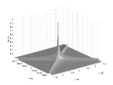
Figure 8: Plot of the real part of the ordinary X-wave, evaluated for $V=1.1\,c$ with $a=3\;$m .

Solutions (15), and in particular the pulse (21), have got an infinite field-depth, and an infinite energy as well. Therefore, as it was done in the Bessel beam case, one should proceed to truncated pulses, originating from a finite aperture. Afterwards, our truncated pulses will keep their spatial shape (and their speed) all along the depth of field

$$Z\;=\;\frac{R}{\tan\theta}\;,$$ (22)

where, as before, $R$ is the aperture radius and $\theta$ the axicon angle.

Some Further Observations — Let us put forth some further observations.

It is not strictly correct to call non-diffractive the localized waves, since diffraction affects, more or less, all waves obeying eq.(1). However, all localized waves (both beams and pulses) possess the remarkable “self-reconstruction” property: That is to say, the localized waves, when diffracting during propagation, do immediately re-build their shape[71, 78, 114] (even after obstacles with size much larger than the characteristic wave-lengths, provided it is smaller —as we know— than the aperture size), due to their particular spectral structure (as it will be shown more in detail in other Chapters of the mentioned book [Localized Waves (J.Wiley; in press]). In particular, the “ideal localized waves” (with infinite energy and depth of field) are able to re-build themselves for an infinite time; while, as we have seen, the finite-energy (truncated) ones can do it, and thus resist the diffraction effects, only along a certain field-depth…

Let us stress again that the interest of the localized waves (especially from the point of view of applications) lies in the circumstance that they are almost non-diffractive, rather than in their group-velocity: From this point of view, Superluminal, luminal, and subluminal localized solutions are equally interesting and suited to important applications.

Actually, the localized waves are not restricted to the (X-shaped, Superluminal) ones corresponding to the integral solution (15) to the wave equation; and, as we were already saying, three classes of localized pulses exist: the Superluminal (with speed $V>c$, the luminal ($V=c$), and the subluminal ($V<c$) ones; all of them with, or without, axial symmetry, and, in any case, corresponding to a unified, single mathematical background.  This issue will be touched again in the present book.  Incidentally, we have elsewhere addressed topics as  (i) the construction of infinite families of generalizations of the classic X-shaped wave [with energy more and more concentrated around the vertex: cf., e.g., Figs.9, taken from ref.[42]]; as  (ii) the behavior of some finite total-energy Superluminal localized solutions (SLS);  (iii) the way for building up new series of SLS’s to the Maxwell equations suitable for arbitrary frequencies and bandwidths, as well as  (iv) questions related with the case of dispersive media: In Chapter 2 of the abovementioned book [Localized Waves (J.Wiley; in press] we shall come back to some (few) of those points.  Let us add that X-shaped waves have been easily produced also in nonlinear media[4], as a further Chapter of the same volume will show.

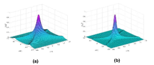
Figure 9: In Fig.(a) it is represented (in arbitrary units) the square magnitude of the “classic”, $X$-shaped Superluminal localized solution (SLS) to the wave equation, with $V=5c$ and $a=0.1\;$m.  Families of infinite SLSs however exists, which generalize the classic $X$-shaped solution; for instance, a family of SLSs obtained[42] by suitably differentiating the classic X-wave: Fig.(b) depicts the first of them (corresponding to the first differentiation) with the same parameters.  As we said, the successsive solutions in such a family are more and more localized around their vertex. Quantity $\rho$ is the distance in meters from the propagation axis $z$, while quantity $\zeta$ is the “$V$-cone” variable[ref.[42]] (still in meters) $\zeta\equiv z-Vt$, with $V\geq c$.  Since all these solutions depend on $z$ only via the variable $\zeta$, they propagate “rigidly”, i.e., as we know, without distortion (and are called “localized”, or non-dispersive, for such a reason). Here we are assuming propagation in the vacuum (or in a homogeneous medium).

A more technical introduction to the subject of localized waves (particularly w.r.t. the Superluminal X-shaped ones) can be found for instance in ref.[55].

APPENDIX:

A HISTORICAL (THEORETICAL AND EXPERIMENTAL) APPENDIX

====================================================

In this mainly “historical” Appendix, written as far as possible in a (partially) self-consistent form, we shall first refer ourselves, from the theoretical point of view, to the most intriguing localized solutions to the wave equation: the Superluminal ones (SLS), and in particular the X-shaped pulses. As a start, we shall recall their geometrical interpretation within SR. Afterwards, to help resolving possible doubts, we shall seize the opportunity, given to us by this Appendix, for presenting a bird’s-eye view of the various experimental sectors of physics in which Superluminal motions seem to appear: In particular, of the experiments with evanescent waves (and/or tunneling photons), and with the SLS’s we are more interested in here. In some parts of this Appendix the propagation-line is called $x$, and no longer $z$, without originating, however, any interpretation problems.

3 INTRODUCTION OF THE APPENDIX

The question of Superluminal ($V^{2}>c^{2}$) objects or waves has a long story. Still in pre-relativistic times, one meets various relevant papers, from those by J.J.Thomson to the interesting ones by A.Sommerfeld. It is well-known, however, that with SR the conviction spread out that the speed $c$ of light in vacuum was the upper limit of any possible speed. For instance, R.C.Tolman in 1917 believed to have shown by his “paradox” that the existence of particles endowed with speeds larger than $c$ would have allowed sending information into the past.  Our problem started to be tackled again only in the fifties and sixties, in particular after the papers[89] by E.C.George Sudarshan et al., and, later on[80, 81], by one of the present authors with R.Mignani et al., as well as —to confine ourselves at present to the theoretical researches— by H.C.Corben and others. The first experimental attempts were performed by T.Alväger et al.

We wish to face the still unusual issue of the possible existence of Superluminal wavelets, and objects —within standard physics and SR, as we said— since at least four different experimental sectors of physics seem to support such a possibility [apparently confirming some long-standing theoretical predictions[1, 14, 89, 81]]. The experimental review will be necessarily short, but we shall provide the reader with further, enough bibliographical information, limited for brevity’s sake to the last century only (i.e., up-dated till the year 2000 only).

4 APPENDIX: HISTORICAL RECOLLECTIONS - THEORY

A simple theoretical framework was long ago proposed[89, 1, 80], merely based on the space-time geometrical methods of SR, which appears to incorporate Superluminal waves and objects, and predict[14] among the others the Superluminal X-shaped waves, without violating the Relativity principles. A suitable choice of the Postulates of SR (equivalent of course to the other, more common, choices) is the following one: (i) the standard Principle of Relativity; and (ii) space-time homogeneity and space isotropy.  It follows that one and only one invariant speed exists; and experience shows that invariant speed to be the light-speed, $c$, in vacuum: The essential role of $c$ in SR being just due to its invariance, and not to the fact that it be a maximal, or minimal, speed. No sub- or Super-luminal objects or pulses can be endowed with an invariant speed: so that their speed cannot play in SR the same essential role played the light-speed $c$ in vacuum. Indeed, the speed $c$ turns out to be a limiting speed: but any limit possesses two sides, and can be approached a priori both from below and from above: See Fig.10.  As E.C.G.Sudarshan put it, from the fact that no one could climb over the Himalayas ranges, people of India cannot conclude that there are no people North of the Himalayas; actually, speed-$c$ photons exist, which are born, live and die just “at the top of the mountain,” without any need for performing the impossible task of accelerating from rest to the light-speed.  [Actually, the ordinary formulation of SR is restricted too much: For instance, even leaving Superluminal speeds aside, it can be easily so widened as to include antimatter[1, 58, 57]].

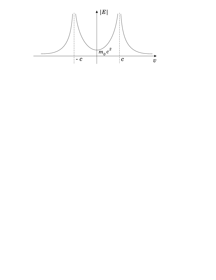
Figure 10: Energy of a free object as a function of its speed.[89, 80, 1]

An immediate consequence is that the quadratic form  $c^{2}{\rm d}t^{2}-{\rm d}\mbox{\boldmath$x$}^{2}\equiv{\rm d}x_{\mu}{\rm d}x^{\mu}$, called ${\rm d}s^{2}$,  with ${\rm d}\mbox{\boldmath$x$}^{2}\equiv{\rm d}x^{2}+{\rm d}y^{2}+{\rm d}z^{2}$,  results to be invariant, except for its sign.  Quantity ${\rm d}s^{2}$, let us emphasize, is the four-dimensional length-element square, along the space-time path of any object.  In correspondence with the positive (negative) sign, one gets the subluminal (Superluminal) Lorentz “transformations” [LT]. The ordinary subluminal LTs are known to leave, e.g., the quadratic forms ${\rm d}x_{\mu}{\rm d}x^{\mu}$, ${\rm d}p_{\mu}{\rm d}p^{\mu}$ and ${\rm d}x_{\mu}{\rm d}p^{\mu}$ exactly invariant, where the $p_{\mu}$ are the component of the energy-impulse four-vector; while the Superluminal LTs, by contrast, have to change (only) the sign of such quadratic forms. This is enough for deducing some important consequences, like the one that a Superluminal charge has to behave as a magnetic monopole, in the sense specified in ref.[1] and refs. therein.

A more important consequence, for us, is —see Fig.11— that the simplest subluminal object, a spherical particle at rest (which appears as ellipsoidal, due to Lorentz contraction, at subluminal speeds $v$), will appear[14, 1, 20] as occupying the cylindrically symmetrical region bounded by a two-sheeted rotation hyperboloid and an indefinite double cone, as in Fig.11(d), for Superluminal speeds $V$. In Fig.11 the motion is along the $x$-axis. In the limiting case of a point-like particle, one obtains only a double cone.

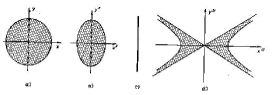
Figure 11: An intrinsically spherical (or pointlike, at the limit) object appears in the vacuum as an ellipsoid contracted along the motion direction when endowed with a speed $v<c$.  By contrast, if endowed with a speed $V>c$ (even if the $c$-speed barrier cannot be crossed, neither from the left nor from the right), it would appear[14, 1] no longer as a particle, but rather as an “X-shaped” wave travelling rigidly: Namely, as occupying the region delimited by a double cone and a two-sheeted hyperboloid —or as a double cone, at the limit–, and moving without distortion in the vacuum, or in a homogeneous medium, with Superluminal speed $V$ [the cotangent square of the cone semi-angle being $(V/c)^{2}-1$]. For simplicity, a space axis is skipped.  This figure is taken from refs.[14, 1]

Such result is simply got by writing down the equation of the world-tube of a subluminal particle, and transforming it by merely changing sign to the quadratic forms entering that equation. Thus, in 1980-1982, it was predicted[14] that the simplest Superluminal object appears (not as a particle, but as a field or rather) as a wave: namely, as an “X-shaped pulse”, the cone semi-angle $\alpha$ being given (with $c=1$) by  ${\rm cotg}\alpha=\sqrt{V^{2}-1}$. Such X-shaped pulses will move rigidly with speed $V$ along their motion direction: In fact, any “X-pulse” can be regarded at each instant of time as the (Superluminal) Lorentz transform of a spherical object, which of course moves in vacuum —or in a homogeneous medium— without any deformation as time elapses.  The three-dimensional picture of Fig.11(d) appears in Fig.12, where its annular intersections with a transverse plane are shown (cf. refs.[14]).  The X-shaped waves here considered are merely the simplest ones: if one starts not from an intrinsically spherical or point-like object, but from a non-spherically symmetric particle, or from a pulsating (contracting and dilating) sphere, or from a particle oscillating back and forth along the motion direction, then their Superluminal Lorentz transforms would result to be more and more complicated. The above-seen “X-waves”, however, are typical for a Superluminal object, so as the spherical or point-like shape is typical, let us repeat, for a subluminal object.

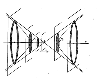
Figure 12: Here we show the intersections of the Superluminal object $T$ represented in Fig.11(d) with planes $P$ orthogonal to its motion line (the $x$-axis).  For simplicity, we assumed again the object to be spherical in its rest-frame, and the cone vertex $C$ to coincide with the origin $O$ for $t=0$.  Such intersections evolve in time so that the same pattern appears on a second plane —shifted by $\Delta x$— after the time $\Delta t=\Delta x/V$.  On each plane, as time elapses, the intersection is therefore predicted by (extended) SR to be a circular ring which, for negative times, goes on shrinking until it reduces to a circle and then to a point (for $t=0$);  afterwards, such a point becomes again a circle and then a circular ring that goes on broadening[BarutNM, 1, 20].  This picture is taken from refs.[BarutNM, 1].  [Notice that, if the object is not spherical when at rest (but, e.g., is ellipsoidal in its own rest-frame), then the axis of $T$ will no longer coincide with $x$, but its direction will depend on the speed $V$ of the tachyon itself].  For the case in which the space extension of the Superluminal object $T$ is finite, see refs.[14]

Incidentally, it has been believed for a long time that Superluminal objects would have allowed sending information into the past; but such problems with causality seem to be solvable within SR. Once SR is generalized in order to include Superluminal objects or pulses, no signal traveling backwards in time is apparently left. For a solution of those causal paradoxes, see refs.[58, RGF, 89] and references therein.

For addressing the problem, even within this elementary context, of the production of an X-shaped pulse like the one depicted in Fig.12 (maybe truncated, in space and in time, by use of a finite antenna radiating for a finite time), all the considerations expounded under point (ii) of the subsection The Ordinary X-shaped Pulse become in order: And, here, we simply refer to them. Those considerations, together with the present ones (related, e.g., to Fig.12), suggest the simplest antenna to consist in a series of concentric annular slits, or transducers [like in Fig.2], which suitably radiate following specific time patterns: See, e.g., refs.[102] and refs. therein.  Incidentally, the above procedure can lead to a very simple type of X-shaped wave.

From the present point of view, it is rather interesting to note that, during the last fifteen years, X-shaped waves have been actually found as solutions to the Maxwell and to the wave equations [let us recall that the form of any wave equations is intrinsically relativistic]. In order to see more deeply the connection existing between what predicted by SR (see, e.g., Figs.11,12) and the localized X-waves mathematically, and experimentally, constructed in recent times, let us tackle below, in detail, the problem of the (X-shaped) field created by a Superluminal electric charge[18], by following a paper recently appeared in Physical Review E.

4.1 The particular X-shaped field associated with a Superluminal charge

It is well-known by now that Maxwell equations admit of wavelet-type solutions endowed with arbitrary group-velocities ($0<v_{\rm g}<\infty$).  We shall again confine ourselves, as above, to the localized solutions, rigidly moving: and, more in particular, to the Superluminal ones (SLS), the most interesting of which resulted to be, as we have seen, X-shaped.  The SLSs have been actually produced in a number of experiments, always by suitable interference of ordinary-speed waves.  In this subsection we show, by contrast, that even a Superluminal charge creates an electromagnetic X-shaped wave, in agreement with what predicted within SR[14, 1]. Namely, on the basis of Maxwell equations, one is able to evaluate the field associated with a Superluminal charge (at least, under the rough approximation of pointlikeness): as announced in what precedes, it results to constitute a very simple example of true X-wave.

Indeed, the theory of SR, when based on the ordinary Postulates but not restricted to subluminal waves and objects, i.e., in its extended version, predicted the simplest X-shaped wave to be the one corresponding to the electromagnetic field created by a Superluminal charge[79, 18].  It seems really important evaluating such a field, at least approximately, by following ref.[18].

The toy-model of a pointlike Superluminal charge — Let us start by considering, formally, a pointlike Superluminal charge, even if the hypothesis of pointlikeness (already unacceptable in the subluminal case) is totally inadequate in the Superluminal case[1].  Then, let us consider the ordinary vector-potential $A^{\mu}$ and a current density $j^{\mu}\equiv(0,0,j_{z};j^{\rm o})$ flowing in the $z$-direction (notice that the motion line is here the axis $z$). On assuming the fields to be generated by the sources only, one has that $A^{\mu}\equiv(0,0,A_{z};\phi)$, which, when adopting the Lorentz gauge, obeys the equation $A^{\mu}=j^{\mu}$.  We can write such non-homogeneous wave equation in the cylindrical co-ordinates $(\rho,\theta,z;t)$; for axial symmetry [which requires a priori that $A^{\mu}=A^{\mu}(\rho,z;t)$], when choosing the “$V$-cone variables” $\zeta\;\equiv\;z-Vt;\ \eta\;\equiv\;z+Vt\;$, with  $V^{2}>c^{2}$, we arrive[18] to the equation

$${\left[-\rho{\partial\over{\partial\rho}}\left(\rho{\partial\over{\partial\rho}}\right)+\frac{1}{\gamma^{2}}\frac{\partial^{2}}{\partial\zeta^{2}}+\frac{1}{\gamma^{2}}\frac{\partial^{2}}{\partial\eta^{2}}-4\frac{\partial^{2}}{\partial\zeta\partial\eta}\right]\;A^{\mu}(\rho,\zeta,\eta)\;=\;j^{\mu}(\rho,\zeta,\eta)}\ ,$$ (23)

where $\mu$ assumes the two values $\mu=3,0$ only, so that  $A^{\mu}\equiv(0,0,A_{z};\phi)$,  and  $\gamma^{2}\equiv[V^{2}-1]^{-1}$.  [Notice that, whenever convenient, we set $c=1$].  Let us now suppose $A^{\mu}$ to be actually independent of $\eta$, namely, $A^{\mu}=A^{\mu}(\rho,\zeta)$.  Due to eq.(23), we shall have $j^{\mu}=j^{\mu}(\rho,\zeta)\,$ too; and therefore $j_{z}=Vj^{0}$ (from the continuity equation), and $A_{z}=V\phi/c$ (from the Lorentz gauge).  Then, by calling $\psi\equiv A_{z}$, we end in two equations[18], which allow us to analyze the possibility and consequences of having a Superluminal pointlike charge, $e$, traveling with constant speed $V$ along the $z$-axis ($\rho=0$) in the positive direction, in which case $j_{z}=e\,V\,\delta(\rho)/{\rho}\;\delta(\zeta)$.  Indeed, one of those two equations becomes the hyperbolic equation

$${\left[-\frac{1}{\rho}\frac{\partial}{\partial\rho}\left(\rho\frac{\partial}{\partial\rho}\right)+\frac{1}{\gamma^{2}}\frac{\partial^{2}}{\partial\zeta^{2}}\right]\,\psi\;=\;eV\,\frac{\delta(\rho)}{\rho}\,\delta(\zeta)}$$ (24)

which can be solved[18] in few steps. First, by applying (with respect to the variable $\rho$) the Fourier-Bessel (FB) transformation  $f(x)\;=\;\displaystyle{\int_{0}^{\infty}\Omega f(\Omega)J_{0}(\Omega x)\,{\rm d}\Omega}$,  quantity $J_{0}(\Omega x)$ being the ordinary zero-order Bessel function.  Second, by applying the ordinary Fourier transformation with respect to the variable $\zeta\,$ (going on, from $\zeta$, to the variable $\omega$).  And, third, by finally performing the corresponding inverse Fourier and FB transformations.  Afterwards, it is enough to have recourse to formulae (3.723.9) and (6.671.7) of ref.[82], still with $\zeta\equiv z-Vt\,$, for being able to write down the solution of eq.(24) in the form

$\left\{\begin{array}[]{clr}\psi(\rho,\zeta)\;=\;0\ \ \ \ \ \ \ \ \ \ \ \ \ \ \ \ \ \ \ \ \ \ \ \ \ \ \ \ \ \ {\rm{for}}\ \ \ 0<\gamma\mid{\zeta}\mid<\rho\\ \\ \displaystyle{\psi(\rho,\zeta)\;=\;\displaystyle{e\frac{V}{\sqrt{\zeta^{2}-\rho^{2}(V^{2}-1)}}}}\ \ \ \ \ {\rm{for}}\ \ \ 0\leq\rho<\gamma\mid{\zeta}\mid\ .\par\end{array}\right.$ (25)

In Fig.13 we show our solution $A_{z}\equiv\psi$, as a function of $\rho$ and $\zeta$, evaluated for $\gamma=1$ (i.e., for $V=c\sqrt{2}$). Of course, we skipped the points in which $A_{z}$ must diverge, namely the vertex and the cone surface.

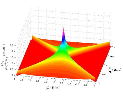
Figure 13: Behaviour of the field $\psi\equiv A_{z}$ generated by a charge supposed to be Superluminal, as a function of $\rho$ and $\zeta\equiv z-Vt$, evaluated for $\gamma=1$ (i.e., for $V=c\sqrt{2}$): According to ref.[18]  [Of course, we skipped the points in which $\psi$ must diverge: namely, the vertex and the cone surface].

For comparison, one may recall that the classic X-shaped solution[19] of the homogeneous wave-equation —which is shown, e.g., in Figs.8,9,12— has the form (with $a>0$):

$\displaystyle{X\;=\;{\frac{V}{\sqrt{(a-i\zeta)^{2}+\rho^{2}(V^{2}-1)}}}}\;.$ (26)

The second one of eqs.(25) includes expression (26), given by the spectral parameter[42, 63] $a=0$, which indeed corresponds to the non-homogeneous case [the fact that for $a=0$ these equations differ for an imaginary unit will be discussed elsewhere].

It is rather important, at this point, to notice that such a solution, eq.(25), does represent a wave existing only inside the (unlimited) double cone ${\cal C}$ generated by the rotation around the $z$-axis of the straight lines $\rho=\pm\gamma\zeta$:  This too is in full agreement with the predictions of the extended theory of SR.  For the explicit evaluation of the electromagnetic fields generated by the Superluminal charge (and of their boundary values and conditions) we confine ourselves here to merely quoting ref.[18].  Incidentally, the same results found by following the above procedure can be obtained by starting from the four-potential associated with a subluminal charge (e.g., an electric charge at rest), and then applying to it the suitable Superluminal Lorentz “transformation”.  One should also notice that this double cone does not have much to do with the Cherenkov cone[1, 79]; and a Superluminal charge traveling at constant speed, in the vacuum, does not lose energy: See, e.g., Fig.14 [which reproduces figure 27 at page 80 of ref.[1]].

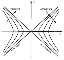
Figure 14: The spherical equipotential surfaces of the electrostatic field created by a charge at rest get transformed into two-sheeted rotation-hyperboloids, contained inside an unlimited double-cone, when the charge travels at Superluminal speed (cf. refs.[18, 1]). This figures shows, among the others, that a Superluminal charge traveling at constant speed, in a homogeneous medium like the vacuum, does not lose energy[79].  Let us mention, incidentally, that this double cone has nothing to do with the Cherenkov cone. [The present picture is a reproduction of figure 27, appeared in 1986 at page 80 of ref.[1]].

Outside the cone ${\cal C}$, i.e., for $0<\gamma\mid{\zeta}\mid<\rho$, we get as expected no field, so that one meets a field discontinuity when crossing the double-cone surface. Nevertheless, the boundary conditions imposed by Maxwell equations are satisfied by our solution (25), since at each point of the cone surface the electric and the magnetic field are both tangent to the cone: also for a discussion of this point we refer to quotation[18].

Here, let us stress that, when $V\rightarrow\infty;\ \gamma\rightarrow 0$, the electric field tends to vanish, while the magnetic field tends to the value $H_{\phi}=-\pi e/\rho^{2}$: This does agree once more with what expected from extended SR, which predicts Superluminal charges to behave (in a sense) as magnetic monopoles. In the present contribution we can only mention such a circumstance, and refer to citations [80, 1, 81, 2], and papers quoted therein.

5 APPENDIX: A GLANCE AT THE EXPERIMENTAL STATE-OF-THE-ART

Extended relativity can allow a better understanding of many aspects also of ordinary physics[1], even if Superluminal objects (tachyons) did not exist in our cosmos as asymptotically free objects.  Anyway, at least three or four different experimental sectors of physics seem to suggest the possible existence of faster-than-light motions, or, at least, of Superluminal group-velocities.  We are going to put forth in the following some information about the experimental results obtained in two of those different physics sectors, with a mere mention of the others.

Neutrinos – First: A long series of experiments, started in 1971, seems to show that the square ${m_{0}}^{2}$ of the mass $m_{0}$ of muon-neutrinos, and more recently of electron-neutrinos too, is negative; which, if confirmed, would mean that (when using a naïve language, commonly adopted) such neutrinos possess an “imaginary mass” and are therefore tachyonic, or mainly tachyonic.[84, 1, 83]  [In extended SR, the dispersion relation for a free Superluminal object becomes  $\omega^{2}-\mbox{\boldmath$k$}^{2}=-\Omega^{2}$,  or  $E^{2}-\mbox{\boldmath$p$}^{2}=-m_{\rm o}^{2}$,  and there is no need at all, therefore, of imaginary masses].

Galactic Micro-quasars – Second: As to the apparent Superluminal expansions observed in the core of quasars[85] and, recently, in the so-called galactic micro-quasars[86], we shall not really deal with that problem, too far from the other topics of this paper; without mentioning that for those astronomical observations there exist orthodox interpretations, based on ref.[87], that are still accepted by the majority of the astrophysicists.  For a theoretical discussion, see ref.[88]. Here, let us mention only that simple geometrical considerations in Minkowski space show that a single Superluminal source of light would appear[88, 1]:  (i) initially, in the “optical boom” phase (analogous to the acoustic “boom” produced by an airplane traveling with constant supersonic speed), as an intense source which suddenly comes into view; and which, afterwards,  (ii) seems to split into TWO objects receding one from the other with speed  $V>2c$ [all of this being similar to what is actually observed, according to refs.[86]].

Evanescent waves and “tunneling photons” – Third: Within quantum mechanics (and precisely in the tunneling processes), it had been shown that the tunneling time —firstly evaluated as a simple Wigner’s “phase time” and later on calculated through the analysis of the wavepacket behavior— does not depend[90] on the barrier width in the case of opaque barriers (“Hartman effect”). This implies Superluminal and arbitrarily large group-velocities $V$ inside long enough barriers: see Fig.15.

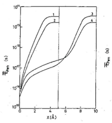
Figure 15: Behaviour of the average “penetration time” (in seconds) spent by a tunnelling wavepacket, as a function of the penetration depth (in ångstroms) down a potential barrier (from Olkhovsky et al., ref.[92]).  According to the predictions of quantum mechanics, the wavepacket speed inside the barrier increases in an unlimited way for opaque barriers; and the total tunnelling time does not depend on the barrier width.[90, 92]

Experiments that may verify this prediction by, say, electrons or neutrons are difficult and rare[91, 65]. Luckily enough, however, the Schroedinger equation in the presence of a potential barrier is mathematically identical to the Helmholtz equation for an electromagnetic wave propagating, for instance, down a metallic waveguide (along the $x$-axis): as shown, e.g., in refs.[115];  and a barrier height $U$ bigger than the electron energy $E$ corresponds (for a given wave frequency) to a waveguide of transverse size lower than a cut-off value. A segment of “undersized” guide —to go on with our example— does therefore behave as a barrier for the wave (photonic barrier), as well as any other photonic band-gap filters.  The wave assumes therein —like a particle inside a quantum barrier— an imaginary momentum or wavenumber and, as a consequence, results exponentially damped along $x$ [see, e.g. Fig.16]: It becomes an evanescent wave (going back to normal propagation, even if with reduced amplitude, when the narrowing ends and the guide returns to its initial transverse size).  Thus, a tunneling experiment can be simulated by having recourse to evanescent waves (for which the concept of group velocity can be properly extended: see the first one of refs.[57]).

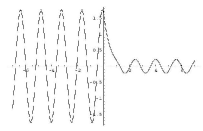
Figure 16: Picture of the damping taking place inside a barrier (from ref.[57]): this damping does reduce the amplitude of the tunnelling wavepacket, imposing a practical limit on the barrier length .

The fact that evanescent waves travel with Superluminal speeds (cf., e.g., Fig.17) has been actually verified in a series of famous experiments. Namely, various experiments, performed since 1992 onwards by G.Nimtz et al. in Cologne[94], by R.Chiao, P.G.Kwiat and A.Steinberg at Berkeley[93], by A.Ranfagni and colleagues in Florence[23], and by others in Vienna, Orsay, Rennes, etcetera, verified that “tunneling photons” travel with Superluminal group velocities [Such experiments raised a great deal of interest[105], also within the non-specialized press, and were reported in Scientific American, Nature, New Scientist, etc.].  Let us add that also extended SR had predicted[ref<] evanescent waves to be endowed with faster-than-$c$ speeds; the whole matter appears to be therefore theoretically selfconsistent.  The debate in the current literature does not refer to the experimental results (which can be correctly reproduced even by numerical simulations[73, 74] based on Maxwell equations only: Cf. Figs.18,19), but rather to the question whether they allow, or do not allow, sending signals or information with Superluminal speed (see, e.g., refs.[66]).

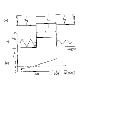
Figure 17: Simulation of tunnelling by experiments with evanescent classical waves (see the text), which were predicted to be Superluminal also on the basis of extended SR[106]. The figure shows one of the measurement results by Nimtz et al.[94]; that is, the average beam speed while crossing the evanescent region ( = segment of undersized waveguide, or “barrier”) as a function of its length. As theoretically predicted[90, 106], such an average speed exceeds $c$ for long enough “barriers”.  Further results appeared in ref.[99], and are reported below: see Figs.20 and 21 in the following .

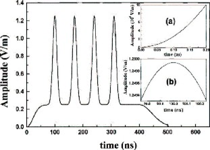
Figure 18: The delay of a wavepacket crossing a barrier (cf., e.g., Fig.17 is due to the initial discontinuity. We then performed suitable numerical simulations[73] by considering an (indefinite) undersized waveguide, and therefore eliminating any geometric discontinuity in its cross-section.  This figure shows the envelope of the initial signal.  Inset (a) depicts in detail the initial part of this signal as a function of time, while inset (b) depicts the gaussian pulse peak centered at $t=100$ ns .

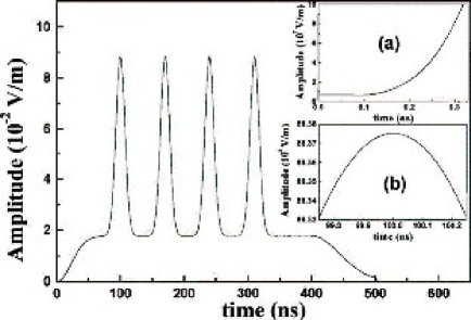
Figure 19: Envelope of the signal in the previous figure (Fig.18) after having traveled a distance $L=32.96$ mm through the mentioned undersized waveguide.  Inset (a) shows in detail the initial part (in time) of such arriving signal, while inset (b) shows the peak of the gaussian pulse that had been initially modulated by centering it at $t=100$ ns.  One can see that its propagation took zero time, so that the signal traveled with infinite speed.  The numerical simulation has been based on Maxwell equations only.  Going on from Fig.18 to Fig.19 one verifies that the signal strongly lowered its amplitute: However, the width of each peak did not change (and this might have some relevance when thinking of a Morse alphabet “transmission”: see the text) .

In the above-mentioned experiments one meets a substantial attenuation of the considered pulses —cf. Fig.16— during tunneling (or during propagation in an absorbing medium): However, by employing “gain doublets”, it has been recently reported the observation of undistorted pulses propagating with Superluminal group-velocity with a small change in amplitude (see, e.g., ref.[97]).

Let us emphasize that some of the most interesting experiments of this series seem to be the ones with TWO or more “barriers” (e.g., with two gratings in an optical fiber, or with two segments of undersized waveguide separated by a piece of normal-sized waveguide: Fig.20).

Figure 20: Very interesting experiments have been performed with TWO successive barriers, i.e., with two evanescence regions: For example, with two gratings in an optical fiber.  This figure[57] refers to the interesting experiment[108] performed with microwaves traveling along a metallic waveguide: the waveguide being endowed with two classical barriers (undersized guide segments). See the text .

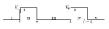
Figure 21: Scheme of the (non-resonant) tunnelling process, through two successive (opaque) quantum barriers. Far from resonances, the (total) phase time for tunnelling through the two potential barriers does depend neither on the barrier widths nor on the distance between the barriers (“generalized Hartman effect”)[100, 91, 98].  See the text.

For suitable frequency bands —namely, for “tunneling” far from resonances—, it was found by us that the total crossing time does not depend on the length of the intermediate (normal) guide: that is, that the beam speed along it is infinite[100, 108, 91].  This does agree with what predicted by Quantum Mechanics for the non-resonant tunneling through two successive opaque barriers[100]: Fig.21.  Such a prediction has been verified first theoretically, by Y.Aharonov et al.[100], and then, a second time, experimentally: by taking advantage of the circumstance that evanescence regions can consist in a variety of photonic band-gap materials or gratings (from multilayer dielectric mirrors, or semiconductors, to photonic crystals). Indeed, the best

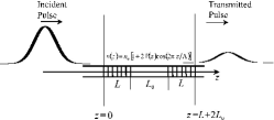
Figure 22: Realization of the quantum-theoretical set-up represented in Fig.21, by using, as classical (photonic) barriers, two gratings in an optical fiber[98].  The corresponding experiment has been performed by Longhi et al.[99]

experimental confirmation has come by having recourse to two gratings in an optical fiber[99]: see Figs.22 and 23; in particular, the rather peculiar (and quite interesting) results represented by the latter.

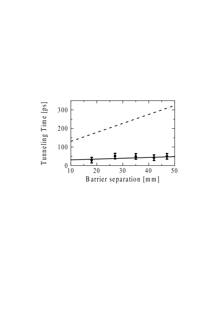
Figure 23: Off-resonance tunnelling time versus barrier separation for the rectangular symmetric DB FBG structure considered in ref.[99] (see Fig.22). The solid line is the theoretical prediction based on group delay calculations; the dots are the experimental points as obtained by time delay measurements [the dashed curve is the expected transit time from input to output planes for a pulse tuned far away from the stopband of the FBGs].  The experimental results[99] do confirm —as well as the early ones in refs.[108]]— the theoretical prediction of a “generalized Hartman Effect”: in particular, the independence of the total tunnelling time from the distance between the two barriers.

We cannot skip a further topic —which, being delicate, should not appear, probably, in a brief overview like this— since it is presently arising more and more interest[97].  Even if all the ordinary causal paradoxes seem to be solvable[58, 1, 57], nevertheless one has to bear in mind that (whenever it is met an object, ${\cal O}$, traveling with Superluminal speed) one may have to deal with negative contributions to the tunneling times[109, 1, 91]: and this should not be regarded as unphysical. In fact, whenever an “object” (particle, electromagnetic pulse,,…) ${\cal O}$ overcomes[58, 1] the infinite speed with respect to a certain observer, it will afterwards appear to the same observer as the “anti-object” $\overline{{\cal O}}$ traveling in the opposite space direction[89, 1, 58].  For instance, when going on from the lab to a frame ${\cal F}$ moving in the same direction as the particles or waves entering the barrier region, the object ${\cal O}$ penetrating through the final part of the barrier (with almost infinite speed[92, 90, 73, 91], like in Figs.15) will appear in the frame ${\cal F}$ as an anti-object $\overline{{\cal O}}$ crossing that portion of the barrier in the opposite space-direction[58, 1, 89]. In the new frame ${\cal F}$, therefore, such anti-object $\overline{{\cal O}}$ would yield a negative contribution to the tunneling time: which could even result, in total, to be negative.  For any clarifications, see the quoted references.  Let us stress, here, that even the appearance of such negative times has been predicted within SR itself, on the basis of its ordinary postulates; and recently confirmed by quantum-theoretical evaluations too[91, 3].  (In the case of a non-polarized beam,, the wave anti-packet coincides with the initial wave packet; if a photon is however endowed with helicity $\lambda=+1$, the anti-photon will bear the opposite helicity $\lambda=-1$).  From the theoretical point of view, besides the above-quoted papers (in particular refs.[91, 90]), see more specifically refs.[110].  On the (very interesting!) experimental side, see the intriguing papers [110].

Let us add here that, via quantum interference effects, it is possible to obtain dielectrics with refraction indices very rapidly varying as a function of frequency, also in three-level atomic systems, with almost complete absence of light absorption (i.e., with quantum induced transparency)[112].  The group velocity of a light pulse propagating in such a medium can decrease to very low values, either positive or negative, with no pulse distortion.  It is known that experiments have been performed both in atomic samples at room temperature, and in Bose-Einstein condensates, which showed the possibility of reducing the speed of light to a few meters per second.  Similar, but negative group velocities, implying a propagation with Superluminal speeds thousands of time higher than the previously mentioned ones, have been recently predicted also in the presence of such an “electromagnetically induced transparency”, for light moving in a rubidium condensate[113].  Finally, let us recall that faster-than-$c$ propagation of light pulses can be (and has been, in same cases) observed also by taking advantage of the anomalous dispersion near an absorbing line, or nonlinear and linear gain lines —as already seen—, or nondispersive dielectric media, or inverted two-level media, as well as of some parametric processes in nonlinear optics (cf., e.g., G.Kurizki et al.’s works).

D)  Superluminal Localized Solutions (SLS) to the wave equations. The “X-shaped waves” – The fourth sector (to leave aside the others) is not less important. It came into fashion again, when it was rediscovered in a series of remarkable works that any wave equation —to fix the ideas, let us think of the electromagnetic case— admit also solutions as much sub-luminal as Super-luminal (besides the luminal ones, having speed $c/n$).  Let us recall, indeed, that, starting from pioneering works as H.Bateman’s, it had slowly become known that all wave equations admit soliton-like (or rather wavelet-type) solutions with sub-luminal group velocities.  Subsequently, also Superluminal solutions started to be written down (in one case[39] just by the mere application of a Superluminal Lorentz “transformation”[1]).

As we know, a remarkable feature of some new solutions of these (which attracted much attention for their possible applications) is that they propagate as localized, non-dispersive pulses, also because of their self-reconstruction property.   It is easy to realize the practical importance, for instance, of a radio transmission carried out by localized beams, independently of their speed; but non-dispersive wave packets can be of use even in theoretical physics for a reasonable representation of elementary particles; and so on.  Incidentally, from the point of view of elementary particles, it can be a source of meditation the fact that the wave equations possess pulse-type solutions that, in the subluminal case, are ball-like (cf. Fig.24): this can have a bearing on the corpuscle/wave duality problem met in quantum physics (besides agreeing, e.g., with Fig.11).

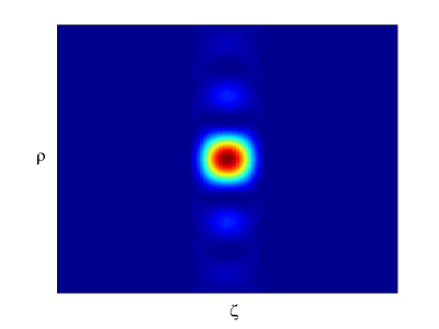
Figure 24: The wave equations possess pulse-type solutions that, in the subluminal case, are ball-like, in agreement with Fig.11.  For comments, see the text.

At the cost of repeating ourselves, let us emphasize once more that, within extended SR, since 1980 it had been found that —whilst the simplest subluminal object conceivable is a small sphere, or a point in the limiting case— the simplest Superluminal objects results by contrast to be (see refs.[14], and Figs.11 and 12 of this paper) an “X-shaped” wave, or a double cone as its limit, which moreover travels without deforming —i.e., rigidly— in a homogeneous medium.  It is not without meaning that the most interesting localized solutions to the wave equations happened to be just the Superluminal ones, and with a shape of that kind.  Even more, since from Maxwell equations under simple hypotheses one goes on to the usual scalar wave equation for each electric or magnetic field component, one expected the same solutions to exist also in the field of acoustic waves, of seismic waves, and of gravitational waves too: and this has already been demonstrated in the literature for the acoustic case.  Actually, such pulses (as suitable superpositions of Bessel beams) were mathematically constructed for the first time, by Lu et al. in Acoustics: and were then called “X-waves” or rather X-shaped waves.

It is indeed important for us that the X-shaped waves have been indeed produced in experiments, both with acoustic and with electromagnetic waves; that is, X-pulses were produced that, in their medium, travel undistorted with a speed larger than sound, in the first case, and than light, in the second case.  In Acoustics, the first experiment was performed by Lu et al. themselves in 1992, at the Mayo Clinic (and their papers received the first 1992 IEEE award).  In the electromagnetic case, certainly more intriguing, Superluminal localized X-shaped solutions were first mathematically constructed (cf., e.g., Fig.25) in refs.[20], and later on

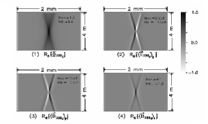
Figure 25: Real part of the Hertz potential and of the field components of the localized electromagnetic (“classic”, axially symmetric) X-shaped wave predicted, and first mathematically constructed for the electromagnetic case, in refs.[20].  For the meaning of the various panels, see the quoted references.  The dimension of each panel is 4 m (in the radial direction) ${\times}$ 2 mm (in the propagation direction).  [The values shown on the right-top corner of each panel represent the maxima and the minima of the images before normalization for display (MKSA units)] .

experimentally produced by Saari et al.[22] in 1997 at Tartu by visible light (Fig.26), and more recently by Mugnai, Ranfagni and Ruggeri at Florence by microwaves[23].  In the theoretical sector the activity has been not less intense, in order to build up —for example— analogous new solutions with finite total energy or more suitable for high frequencies, on one hand, and localized solutions Superluminally propagating even along a normal waveguide (cf. Fig.27), on another hand, and so on.

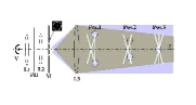
Figure 26: Scheme of the experiment by Saari et al., who announced (PRL of 24 Nov.1997) the production in optics of the beams depicted in the previous Fig.25.   In the present figure one can see what it was shown by the experimental results: Namely, that the “X-shaped” waves are Superluminal: indeed, they, running after plane waves (the latter regularly traveling with speed $c$), do catch up with the considered plane waves.  An analogous experiment has been later on performed with microwaves at Florence by Mugnai, Ranfagni and Ruggeri (PRL of 22 May 2000).

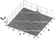
Figure 27: In this figure a couple of elements are depicted of one of the trains of X-shaped pulses, mathematically constructed in ref.[67], which propagate down a coaxial guide (in the TM case): This picture is just taken from ref.[67],  but analogous X-pulses exist (with infinite or finite total energy) for propagation along a cylindrical, normal-sized metallic waveguide].

Let us eventually recall the problem of producing an X-shaped Superluminal wave like the one in Fig.12, but truncated —of course– in space and in time (by use of a finite antenna, radiating for a finite time): in such a situation, the wave is known to keep its localization and Superluminality only till a certain depth of field [i.e., as long as they are fed by the waves arriving (with speed $c$) from the antenna], decaying abruptly afterwards.[40, 42]  Let us add that various authors, taking account, e.g., of the time needed for fostering such Superluminal waves, have concluded that these localized Superluminal pulses are unable to transmit information faster than $c$.  Many of these questions have been discussed in what precedes; for further details, see the second of refs.[20].

Anyway, the existence of the X-shaped Superluminal (or Super-sonic) pulses seem to constitute, together, e.g., with the Superluminality of evanescent waves, a confirmation of extended SR: a theory[1] based on the ordinary postulates of SR and that consequently does not appear to violate any of the fundamental principles of physics.  It is curious moreover, that one of the first applications of such X-waves (that takes advantage of their propagation without deformation) has been accomplished in the field of medicine, and precisely —as we know— of ultrasound scanners[24, 25]; while the most important applications of the (subluminal!) Frozen Waves will very probably affect, once more, human health problems like the cancerous ones.

Acknowledgements

For useful discussions they are grateful, among the others, to R.Bonifacio, M.Brambilla, R.Chiao, C.Cocca, C.Conti, A.Friberg, G.Degli Antoni, F.Fontana, G.Kurizki, M.Mattiuzzi, P.Milonni, P.Saari, A.Shaarawi, R.Ziolkowski, and particularly A.Loredo and M.Tygel.

References

- [1] E.Recami: “Classical Tachyons and Possible Applications”, Rivista Nuovo Cim. 9(6) (1986) 1–178, issue no.6; and refs. therein.
- [2] E.Recami and R.Mignani: “Magnetic Monopoles and Tachyons in Special Relativity”, Physics Letters B62 (1976) 41-43.
- [3] V.Petrillo and L.Refaldi: Phys. Rev. A67 (2003) 012110; V.Petrillo and L.Refaldi: Opt. Commun. 186 (2000) 35. See also L.Refaldi: MSc thesis (V.Petrillo, R.Bonifacio, E.Recami supervisors), Phys. Dept., Milan Univ., 2000.
- [4] C.Conti, S.Trillo, G.Valiulis, A.Piskarkas, O. van Jedrkiewicz, J.Trull and P.Di Trapani, “Non-linear electromagnetic X-waves”, Phys. Rev. Lett. 90 (2003) 170406.
- [5] See, e.g., M.Zamboni-Rached, “Localized waves in diffractive/dispersive media”, PhD Thesis, Aug.2004, Universidade Estadual de Campinas, DMO/FEEC (supervised by H.E.H.Figueroa).
- [6] M.Born and E.Wolf: Principles of Optics — Electromagnetic Theory of Propagation, Interference and Diffraction of Light, 6th edition (Cambridge Univ. Press; Cambridge, 1998).
- [7] H.A.Willebrand and B.S.Ghuman: “Fiber Optics Without Fiber”, IEEE Spectrum, vol.38, no.8 (2001).
- [8] J.W.Goodman: Introduction to Fourier Optics, 2nd edition (McGraw-Hill; New York, 1996).
- [9] S.Okazaki: “Resolution limits of optical lithography”, Journal of Vacuum Science and Technology B, vol.9, pp.2829-2833 (1991).
- [10] T.Ito and S.Okazaki: “Pushing the limits of lithography”, Nature, vol.406, pp.1027-1031 (2000).
- [11] A.Ashkin, J.M.Dziedzic, J.E.Bjorkholm and S.Chu: “Observation of a single-beam gradient force optical trap for dielectric particles”, Optics Letters, vol.11, pp.288-290 (1986).
- [12] J.E.Curtis, B.A.Koss and D.G.Grier: “Dynamic holographic optical tweezers”, Optics Communications, vol.207, pp.169-175 (2002).
- [13] G.P.Agrawal: Nonlinear Fiber Optics, 2nd edition (Acad. Press; New York, 1995).
- [14] A.O.Barut, G.D.Maccarrone and E.Recami: “On the Shape of Tachyons”, Nuovo Cimento A, vol.71, pp.509-533 (1982); and refs. therein. Cf. also E.Recami and G.D.Maccarrone: Lett. Nuovo Cim. 28 (1980) 151-157 ; ibidem 37 (1983) 345-352; P.Caldirola, G.D.Maccarrone and E.Recami: Lett. Nuovo Cim. 29 (1980) 241-250; G.D.Maccarrone, M.Pavsic and E.Recami: Nuovo Cimento B73 (1983) 91-111.
- [15] J.A.Stratton: Electromagnetic Theory, page 356 (McGraw-Hill; New York, 1941).
- [16] R.Courant and D.Hilbert: Methods of Mathematical Physics, vol.2, p.760 (J.Wiley; New York, 1966).
- [17] H.Bateman: Electrical and Optical Wave Motion (Cambridge Univ.Press; Cambridge, 1915).
- [18] E.Recami, M.Zamboni-Rached and C.A.Dartora: “The X-shaped, localized field generated by a Superluminal electric charge” [e-print physics/0210047], Physical Review E, vol.69, no.027602 (2004) [4 pages].
- [19] J.-y. Lu and J.F.Greenleaf: “Nondiffracting X-waves: Exact solutions to free-space scalar wave equation and their finite aperture realizations”, IEEE Transactions in Ultrasonics Ferroelectricity and Frequency Control, vol.39, pp.19-31 (1992); and refs. therein.
- [20] J.-y.Lu, J.F.Greenleaf and E.Recami, “Limited diffraction solutions to Maxwell (and Schroedinger) equations” [Lanl Archives e-print physics/9610012], Report INFN/FM–96/01 (I.N.F.N.; Frascati, Oct.1996); E.Recami: “On localized X-shaped Superluminal solutions to Maxwell equations,” Physica A, vol.252, pp.586-610 (1998); and refs. therein. See also R.W.Ziolkowski, I.M.Besieris and A.M.Shaarawi, J. Opt. Soc. Am. A10, 75 (1993); J. Phys. A: Math.Gen. 33, 7227-7254 (2000).
- [21] J.-y. Lu and J.F.Greenleaf: “Experimental verification of nondiffracting X-waves”, IEEE Transactions in Ultrasonics Ferroelectricity and Frequency Control, vol.39, pp.441-446 (1992).
- [22] P.Saari and K.Reivelt: “Evidence of X-shaped propagation-invariant localized light waves,” Physical Review Letters, vol.79, pp.4135-4138 (1997).
- [23] D.Mugnai, A.Ranfagni, and R.Ruggeri: “Observation of Superluminal behaviors in wave propagation,” Physical Review Letters, vol.84, pp.4830-4833 (2000).
- [24] J.-y. Lu, H.-H.Zou and J.F.Greenleaf: “Biomedical ultrasound beam forming”, Ultrasound in Medicine and Biology, vol.20, pp.403-428 (1994).
- [25] J.-y. Lu, H.-h.Zou and J.F.Greenleaf: “Producing deep depth of field and depth independent resolution in NDE with limited diffraction beams”, Ultrasonic Imaging, vol.15, pp.134-149, 1993.
- [26] V.Garcés-Chavez, D.McGloin, H.Melville, W.Sibbett and K.Dholakia: “Simultaneous micromanipulation in multiple planes using a self-reconstructing light beam”, Nature, vol.419, pp.145-147 (2002).
- [27] D.McGloin, V.Garcés-Chavez and K.Dholakia: “Interfering Bessel beams for optical micromanipulation”, Optics Letters, Vol.28, pp.657-659 (2003).
- [28] M.P.MacDonald et al.: “Creation and manipulation of three-dimensional optically trapped structures”, Science, Vol.296, pp.1101-1103 (2002).
- [29] J.Arlt, V.Garcés-Chavez, W.Sibbett and K.Dholakia: “Optical micromanipulation using a Bessel light beam”, Optics Communications, vol.197, pp.239-245 (2001).
- [30] D.P.Rhodes, G.P.T.Lancaster, J.Livesey, D.McGloin, J.Arlt and K.Dholakia: “Guiding a cold atomic beam along a co-propagating and oblique hollow light guide”, Optics Communications, vol.214, pp.247-254 (2002).
- [31] J.Fan, E.Parra and H.M.Milchberg: “Resonant self-trapping and absorption of intense Bessel beams”, Physical Review Letters, vol.84, pp.3085-3088 (2000).
- [32] J.Arlt, T.Hitomi and K.Dholakia: “Atom guiding along Laguerre-Gaussian and Bessel light beams”, Applied Physics B, vol.71, pp.549-554 (2000).
- [33] M.Erdélyi, Z.L.Horvath, G.Szabo, Zs.Bor, F.K.Tittell, J.R.Cavallaro and M.C.Smayling: “Generation of diffraction-free beams for applications in optical Microlithography”, Journal of Vacuum Science and Technology B, vol.15, pp.287-292 (1997), and refs. therein.
- [34] R.M.Herman and T.A.Wiggins: “Production and uses of diffractionless beams,” Journal of the Optical Society of America A, vol.8, pp.932-942 (1991).
- [35] R.W.Ziolkowski: “Localized transmission of electromagnetic energy,” Physical Review A, vol.39, pp.2005-2033 (1989).
- [36] R.W.Ziolkowski: ”Localized wave physics and engineering,” Physical Review A, vol.44, pp.3960-84 (1991).
- [37] J.-y. Lu and H.Shiping: “Optical X wave communications”, Optics Communications, vol.161, pp.187-192 (1999).
- [38] A.Vasara, J.Turunen and A.T.Friberg: “Realization of general nondiffracting beams with computer-generated holograms”, Journal of the Optical Society of America A, vol.6, pp.1748-1754 (1989); J.Salo, J.Fagerholm, A.T.Friberg and M.M.Salomaa, “Nondiffracting bulk-acoustic X-waves in crystals”, Phys. Rev. Lett. 83 (1990) 1171-74; J.Salo, A.T.Friberg and M.M.Salomaa, “Orthogonal X-waves”, J. Phys. A: Math. Gen. 34 (2001) 9319-27.
- [39] See, e.g., A.O.Barut and H.C.Chandola, “Localized tachyonic wavelet solutions of the wave equation”, Physics Letters A, vol.180, pp.5-8 (1993); and refs. therein.
- [40] J.Durnin, J.J.Miceli and J.H.Eberly: “Diffraction-free beams,” Physical Review Letters, vol. 58, pp.1499-1501 (1987).
- [41] J.Durnin: “Exact solutions for nondiffracting beams: I. The scalar theory,” Journal of the Optical Society of America A, vol.4, pp.651-654 (1987).
- [42] M.Zamboni-Rached, E.Recami and H.E.Hernández-Figueroa: “New localized Superluminal solutions to the wave equations with finite total energies and arbitrary frequencies,” European Physical Journal D, vol.21, pp.217-228 (2002).
- [43] W.Ziolkowski, I.M.Besieris and A.M.Shaarawi: “Aperture realizations of exact solutions to homogeneous wave-equations”, J. Opt. Soc. Am. A10 (1993) 75, Sects.5 and 6.
- [44] R.P.MacDonald, J.Chrostowski, S.A.Boothroyd and B.A.Syrett: “Holographic Formation of a Diode Laser Non-Diffracting Beam”, Applied Optics, vol.32, pp.6470-6474 (1983).
- [45] M.Zamboni-Rached: “Stationary optical wave fields with arbitrary longitudinal shape by superposing equal frequency Bessel beams: Frozen Waves”, Optics Express, vol.12, pp.4001-4006 (2004).
- [46] M.Zamboni-Rached, E.Recami and H.E.Hernández-Figueroa: “Theory of ‘Frozen Waves’ [e-print physics/0502105], Journal of the Optical Society of America A, vol.11, pp.2465-2475 (2005).
- [47] A.O.Barut and A.Grant: “Quantum particle-like configurations of the electromagnetic field”, Found. Phys. Lett., vol.3, pp.303-310 (1990).
- [48] A.O.Barut and A.J.Bracken: “Particle-like configurations of the electromagnetic field: an extension of de Broglie’s ideas”, Found. Phys., vol.22, pp.1267-1285 (1992).
- [49] J.N.Brittingham: “Focus wave modes in homogeneous Maxwell’s equations: transverse electric mode,” J. Appl. Phys., vol.54, pp.1179-1189 (1983).
- [50] A.Sezginer: “A general formulation of focus wave modes”, J. Appl. Phys., vol.57, pp.678-683 (1985).
- [51] I.M.Besieris, A.M.Shaarawi and R.W.Ziolkowski: “A bidirectional traveling plane wave representation of exact solutions of the scalar wave equation”, J. Math. Phys., vol.30, pp.1254-1269 (1989).
- [52] A.M.Shaarawi, I.M.Besieris and R.W.Ziolkowski: “A novel approach to the synthesis of nondispersive wave packet solutions to the Klein-Gordon and Dirac equations”, J. Math. Phys., vol.31, pp.2511-2519 (1990).
- [53] R.W.Ziolkowski, I.M.Besieris and A.M.Shaarawi: “Aperture realizations of exact solutions to homogeneous wave equations”, Journal of the Optical Society of America A, vol.10, pp.75-87 (1993).
- [54] R.Donnelly and R.W.Ziolkowski: “Designing localized waves”, Proceedings of the Royal Society of London, A, vol.440, pp.541-565 (1993).
- [55] E.Recami, M.Zamboni-Rached, K.Z.Nobrega, C.A.Dartora and H.E.Hernández-Figueroa: “On the Localized Superluminal Solutions to the Maxwell Equations”, IEEE Journal of Selected Topics in Quantum Electronics, Vol.9, pp.59-73 (2003).
- [56] E.Recami: “Superluminal motions? A bird’s-eye view of the experimental status-of-the-art”, Found. Phys., vol.31, pp.1119-1135 (2001).
- [57] E.Recami, F.Fontana and R.Garavaglia: “Superluminal motions and Special Relativity: A discussion of recent experiments”, Int. J. Mod. Phys. A, vol.15, pp.2793-2812 (2000). Cf. also R.Garavaglia, Thesis work (Dip. Sc. Informazione, Università statale di Milano; Milan, 1998; G.Degli Antoni and E.Recami supervisors); and M.Pavsic and E.Recami: “Charge Conjugation and Internal Space-Time Symmetries”, Lett. Nuovo Cimento 34 (1982) 357-362.
-
[58]
E.Recami: “Tachyon Mechanics and Causality; A Systematic
Thorough Analysis of the Tachyon Causal Paradoxes”, Foundations of
Physics 17 (1987) 239-296. See also E.Recami: “The Tolman-Regge
Antitelephone Paradox: Its Solution by Tachyon Mechanics”, Lett. Nuovo
Cimento 44 (1985) 587-593.
Lett. Nuovo Cimento 44 (1985) 587-593; and G.D.Maccarrone and E.Recami: “Two-Body Interactions through Tachyon Exchange”, Nuovo Cimento A57 (1980) 85-101. - [59] A.T.Friberg, J.Fagerholm and M.M.Salomaa: “Space-frequency analysis of nondiffracting pulses”, Optics Communications, vol.136, pp.207-212 (1997).
- [60] R.W.Ziolkowski, I.M.Besieris and A.M.Shaarawi: “Aperture realizations of exact solutions to homogeneous wave equations”, Journal of the Optical Society of America A, vol.10, pp.75-87 (1993).
- [61] A.M.Shaarawi and I.M.Besieris: “On the Superluminal propagation of X-shaped localized waves”, J. Phys. A, vol.33, pp.7227-7254 (2000).
- [62] A.M.Shaarawi and I.M.Besieris: “Relativistic causality and Superluminal signalling using X-shaped localized waves”, J. Phys. A, vol.33, pp.7255-7263, 2000; and refs. therein.
- [63] M.Zamboni-Rached, K.Z.Nobrega, H.E.Hernández-Figueroa and E.Recami: “Localized Superluminal solutions to the wave equation in (vacuum or) dispersive media, for arbitrary frequencies and with adjustable bandwidth”, Optics Communications, vol.226, pp.15-23 (2003).
- [64] M.Zamboni-Rached, E.Recami and F.Fontana: “Localized Superluminal solutions to Maxwell equations propagating along a normal-sized waveguide,” Physical Review E, vol.64, no.066603 (2001) [6 pages].
- [65] V.S.Olkhovsky, E.Recami and A.K.Zaichenko: “Resonant and non-resonant tunneling through a double barrier”, Europhysics Letters 70 (2005) 712-718.
- [66] See, for instance, P.W.Milonni, J. Phys. B, vol.35 (2002) R31-R56; G.Nimtz and A.Haibel, Ann. der Phys., vol.11 (2002) 163-171; R.W.Ziolkowski, Phys. Rev. E, vol.63 (2001) 046604; A.M.Shaarawi and I.M.Besieris, J. Phys. A, vol.33 (2000) 7227-7254; 7255-7263; E.Recami, F.Fontana and R.Garavaglia, ref.[57] and refs. therein.
- [67] M.Zamboni-Rached, K.Z.Nobrega, E.Recami and H.E.Hernández-Figueroa: “Superluminal X-shaped beams propagating without distortion along a coaxial guide,” Physical Review, vol.E66, no.036620 (2002) [10 pages]; and refs. therein.
- [68] C.A.Dartora, M.Zamboni-Rached, K.Z.Nobrega, E.Recami and H.E.Hernández-Figueroa: “General formulation for the analysis of scalar diffraction-free beams using angular modulation: Mathieu and Bessel Beams”, Optics Communications, vol.222, pp.75-80 (2003).
- [69] J.Durnin, J.J.Miceli and J.H.Eberly: “Comparison of Bessel and Gaussian beams”, Optics Letters, vol.13, pp.79-80 (1988).
- [70] P.L.Overfelt and C.S.Kenney: “Comparison of the propagation characteristics of Bessel, Bessel-Gauss, and gaussian beams diffracted by a circular aperture”, Journal of the Optical Society of America A, vol.8, pp.732-745 (1991).
- [71] Z.Bouchal, J.Wagner and M.Chlup: “Self-reconstruction of a distorted nondiffracting beam”, Optics Communications, vol.151, pp.207-211 (1998).
- [72] Ettore Majorana - Notes on Theoretical Physics, edited by S.Esposito, E.Majorana jr., A. van der Merwe and E.Recami (Kluwer; Dordrecht and N.Y., Nov.2003), 512 pages.
- [73] A.P.L.Barbero, H.E.Hernández F., and E.Recami, “On the propagation speed of evanescent modes”, Phys. Rev. E, vol.62, 8628 (2000), and refs. therein. Cf. also A.M.Shaarawi and I.M.Besieris, Phys. Rev. E, vol.62, 7415 (2000).
- [74] H.M.Brodowsky, W.Heitmann and G.Nimtz, Phys. Lett. A, vol.222, 125 (1996).
- [75] M. Zamboni-Rached, H. E. Hernández-Figueroa and E.Recami: “Chirped optical X-shaped pulses in material media”, J. Opt. Soc. Am. A21 (2004) 2455-2463.
- [76] A.C.Newell and J.V.Molone, Nonlinear Optics (Addison & Wesley; Redwood City, CA, 1992).
- [77] M.Zamboni-Rached, “Diffraction-attenuation resistant beams in absorbing media”, Opt. Express 14 (2006) 1804-1809 [paper chosen for mention also in the Virtual Journal for Biomedical Optics, and in Laser Focus World, Section “new bracks”].
- [78] R.Grunwald et al., “Generation and characterization of spatially and temporally localized few-cycle optical wavepackets”, Phys. Rev. A67 (2003) 063820; R.Grunwald, U.Griebner, U.Neumann and V.Kebbel, “Self-recontruction of ultrashort-pulse Bessel-like X-waves”, CLEO/QELS Conference (San Francisco; 2004), paper no.CMQ7; R.Grunwald et al., “Ultrabroadband spectral transfer in extended focal zones: truncated few-cycle Bessel-Gauss beams”, CLEO Conference (Baltimore, 2005), paper CTuAA6.
- [79] See E.Recami: ref.[1], pp.80-81; and figure 27 and refs. therein; and R.Folman and E.Recami: Found. Phys. Lett. 8 (1995) 127-134.
- [80] E.Recami and R.Mignani: Rivista Nuovo Cim. 4 (1974) 209-290, E398.
- [81] See, e.g., E.Recami (editor): Tachyons, Monopoles, and Related Topics (North-Holland; Amsterdam; 1978), pp.X + 285.
- [82] I.S.Gradshteyn and I.M.Ryzhik: Integrals, Series and Products, 4th edition (Ac.Press; New York, 1965).
- [83] E.Giannetto, G.D.Maccarrone, R.Mignani and E.Recami, Phys. Lett. B178 (1986) 115-120 (1986) and refs. therein.
- [84] Cf. M.Baldo Ceolin, “Review of neutrino physics”, invited talk at the XXIII Int. Symp. on Multiparticle Dynamics (Aspen, CO; Sept.1993); E.W.Otten, Nucl. Phys. News, vol.5, 11 (1995). From the theoretical point of view, see, e.g., E.Giannetto et al., ref.[83] and refs. therein; S.Giani, “Experimental evidence of Superluminal velocities in astrophysics and proposed experiments”, CP458, in Space Technology and Applications International Forum 1999, ed. by M.S.El-Genk (A.I.P.; Melville, 1999), pp.881-888.
- [85] See, e.g., J.A.Zensus and T.J.Pearson (editors), Superluminal Radio Sources (Cambridge Univ.Press; Cambridge, UK, 1987).
- [86] I.F.Mirabel and L.F.Rodriguez, “A Superluminal source in the Galaxy”, Nature, vol.371, 46 (1994) [with an editorial comment, “A galactic speed record”, by G.Gisler, at page 18 of the same issue]; S.J.Tingay et al., “Relativistic motion in a nearby bright X-ray source”, Nature, vol.374, 141 (1995).
- [87] M.J.Rees, Nature, vol.211, 46 (1966); A.Cavaliere, P.Morrison and L.Sartori, Science, vol.173, 525 (1971).
- [88] E.Recami, A.Castellino, G.D.Maccarrone and M.Rodonò, “Considerations about the apparent Superluminal expansions observed in astrophysics”, Nuovo Cimento B93, 119 (1986). Cf. also R.Mignani and E.Recami, Gen. Relat. Grav., 5 (1974) 615.
- [89] See, e.g., O.M.Bilaniuk, V.K.Deshpande and E.C.G.Sudarshan, Am. J. Phys., vol.30, 718 (1962).
- [90] V.S.Olkhovsky and E.Recami, “Recent Developments in the Time Analysis of Tunnelling Processes”, Physics Reports 214 (1992) 339-357, issue n 6, and refs. therein: In particular T.E.Hartman, J. Appl. Phys., vol.33, 3427 (1962); L.A.MacColl, Phys. Rev., vol.40 (1932) 621. See also V.S.Olkhovsky, E.Recami, F.Raciti and A.K.Zaichenko, J. de Phys.-I, vol.5, 1351-1365 (1995); V.S.Olkhovsky, E.Recami and J.Jakiel, “Unified time analysis of photon and nonrelativistic particle tunneling” [Report INFN/FM-01/01 (Infn; Frascati, Apr.2001)], e-print quant-ph/0102007; P.W.Milonni, J. Phys. B, vol.35 (2002) R31-R56.
- [91] V.S.Olkhovsky, E.Recami and J.Jakiel, “Unified time analysis of photon and nonrelativistic particle tunneling”, Physics Reports 398 (2004) 133-178.
- [92] V.S.Olkhovsky, E.Recami, F.Raciti and A.K.Zaichenko, J. de Phys.-I, vol.5, 1351-1365 (1995).
- [93] A.M.Steinberg, P.G.Kwiat and R.Y.Chiao, Phys. Rev. Lett., vol.71, 708 (1993), and refs. therein; Scient. Am., vol.269(2), 38 (1993), issue no.2. For a review, see, e.g., R.Y.Chiao and A.M.Steinberg, in Progress in Optics, ed. by E.Wolf (Elsevier; Amsterdam, 1997), p.345. Cf. also Y.Japha and G.Kurizki, Phys. Rev. A, vol.53, 586 (1996).
- [94] G.Nimtz and A.Enders, J. de Physique-I, vol.2, 1693 (1992); vol.3, 1089 (1993); vol.4, 1379 (1994); Phys. Rev. E, vol.48, 632 (1993); H.M.Brodowsky, W.Heitmann and G.Nimtz, J. de Physique-I, vol.4, 565 (1994); Phys. Lett. A, vol.222, 125 (1996); vol.196, 154 (1994). For a review, see, e.g., G.Nimtz and W.Heitmann, Prog. Quant. Electr., vol.21, 81 (1997).
- [95] A.Ranfagni, P.Fabeni, G.P.Pazzi and D.Mugnai, Phys. Rev. E, vol.48, 1453 (1993); Ch.Spielmann, R.Szipocs, A.Stingl and F.Krausz, Phys. Rev. Lett., vol.73, 2308 (1994), Ph.Balcou and L.Dutriaux, Phys. Rev. Lett., vol.78, 851 (1997); V.Laude and P.Tournois, J. Opt. Soc. Am. B, vol.16, 194 (1999).
- [96] Scientific American (Aug. 1993); Nature (Oct.21, 1993); New Scientist (Apr. 1995); Newsweek (19 June 1995).
- [97] L.J.Wang, A.Kuzmich and A.Dogariu, Nature, vol.406 (2000) 277.
- [98] E.Recami: “Superluminal motions? A bird-eye view of the experimental situation”, Found. Phys. 31 (2001) 1119-1135; V.S.Olkhovsky, E.Recami and G.Salesi: “Tunneling through two successive barriers and the Hartman (Superluminal) effect”, Lanl archives e-print quant-ph/0002022]; Europhys. Lett. 57 (2002) 879-884. Cf. also E.Recami, M.Z.Rached, K.Z.Nobrega, C.A.Dartora and H.E.Hernandez F.: ”On the localized superluminal solutions to the Maxwell equations”, IEEE Journal of Selected Topics in Quantum Electronics 9(1) (2003) 59-73; E.Recami: “Superluminal tunnelling through successive barriers: Does quantum mechanics predict infinite group velocities?”, J. Mod. Optics 51 (2004) 913-923.
- [99] S.Longhi, P.Laporta, M.Belmonte and E.Recami: “Measurement of Superluminal optical tunneling times in double-barrier photonic bandgaps”, Phys. Rev. E, vol.65 (2002) 046610.
- [100] V.S.Olkhovsky, E.Recami and G.Salesi, Europhysics Letters 57 (2002) 879-884; “Tunneling through two successive barriers and the Hartman (Superluminal) effect”, LANL archives e-print quant-ph/0002022; Y.Aharonov, N.Erez and B.Reznik, Phys. Rev. A, vol.65 (2002) 052124; S.Esposito: Phys. Rev. E67 (2003) 016609. Cf. also E.Recami: “Superluminal tunnelling through successive barriers: Does quantum mechanics predict infinite group velocities?”, J. Mod. Optics 51 (2004) 913-923.
- [101] L.J.Wang, A.Kuzmich and A.Dogariu, Nature, vol.406 (2000) 277; M.W.Mitchell and R.Y.Chiao, Phys. Lett. A, vol.230 (1997) 133-138. See also S.Chu and Wong W., Phys. Rev. Lett., vol.48 (1982) 738; B.Segard and B.Macke, Phys. Lett. A, vol.109 (1985) 213-216; B.Macke et al., J. Physique, vol.48 (1987) 797-808; G.Nimtz, Europ. Phys. J., B (to appear as a Rapid Note).
- [102] M. Zamboni-Rached, “Analytical expressions for the longitudinal evolution of nondiffracting pulses truncated by finite apertures,” J. Opt. Soc. Am. A 23 (2006) 2166-2176.
- [103] F.Selleri, talk presented at the “2nd Cracow-Clausthal workshop on Extensions of quantum theory”, Krakow, 2000 (unpublished); and in F.Selleri, “Lezioni di relatività da Einstein all’etere di Lorentz” (Progedit pub.; Bari, 2003).
- [104] A.Ranfagni, P.Fabeni, G.P.Pazzi and D.Mugnai, Phys. Rev. E, vol.48, 1453 (1993); Ch.Spielmann, R.Szipocs, A.Stingl and F.Krausz, Phys. Rev. Lett., vol.73, 2308 (1994), Ph.Balcou and L.Dutriaux, Phys. Rev. Lett., vol.78, 851 (1997); V.Laude and P.Tournois, J. Opt. Soc. Am. B, vol.16, 194 (1999).
- [105] Scientific American (Aug. 1993); Nature (Oct.21, 1993); New Scientist (Apr. 1995); Newsweek (19 June 1995).
- [106] Ref.[1], p.158 and pp.116-117. Cf. also D.Mugnai, A.Ranfagni, R.Ruggeri, A.Agresti and E.Recami, Phys. Lett. A, vol.209, 227 (1995).
- [107] H.M.Brodowsky, W.Heitmann and G.Nimtz, Phys. Lett. A, vol.222, 125 (1996).
- [108] G.Nimtz, A.Enders and H.Spieker, in Wave and Particle in Light and Matter, ed. by A.van der Merwe and A.Garuccio (Plenum; New York, 1993); J. de Physique-I, vol.4, 565 (1994). See also A.Enders and G.Nimtz, Phys. Rev. B, vol.47, 9605 (1993).
- [109] V.S.Olkhovsky, E.Recami, F.Raciti and A.K.Zaichenko, ref.[[12]], page 1361 and refs. therein; E.Recami, F.Fontana and R.Garavaglia, ref.[82], page 2807; and ref.[91], page 152.
- [110] R.Y.Chiao, A.E.Kozhekin A.E., and G.Kurizki, Phys. Rev. Lett., vol.77, 1254 (1996); E.L.Bolda et al., Phys. Rev. A, vol.48 (1993) 3890; C.G.B.Garret and D.E.McCumber, Phys. Rev. A, vol.1, 305 (1970).
- [111] S.Chu and Wong W., Phys. Rev. Lett., vol.48 (1982) 738; B.Segard and B.Macke, Phys. Lett. A, vol.109 (1985) 213-216; B.Macke et al., J. Physique, vol.48 (1987) 797-808; M.W.Mitchell and R.Y.Chiao, Phys. Lett. A, vol.230 (1997) 133-138; L.J.Wang, A.Kuzmich and A.Dogariu, Nature, vol.406 (2000) 277; G.Nimtz, Europ. Phys. J., B, vol.7, 523-525 (1999).
- [112] G.Alzetta, A.Gozzini, L.Moi and G.Orriols: Nuovo Cimento B, vol.36, 5 (1976).
- [113] M.Artoni, G.C.La Rocca, F.S.Cataliotti and F.Bassani: Phys. Rev. A, vol.63, no.023805 (2001).
- [114] M.Zamboni-Rached: private communications (2003).
- [115] See, e.g., R.Y.Chiao, P.G.Kwiat and A.M.Steinberg, Physica B, vol.175, 257 (1991); A.Ranfagni, D.Mugnai, P.Fabeni and G.P.Pazzi, Appl. Phys. Lett., vol.58, 774 (1991); Th.Martin and R.Landauer, Phys. Rev. A, vol.45, 2611 (1992); Y.Japha and G.Kurizki, Phys. Rev. A, vol.53, 586 (1996). Cf. also G.Kurizki, A.E.Kozhekin and A.G.Kofman, Europhys. Lett., vol.42, 499 (1998); G.Kurizki, A.E.Kozhekin, A.G.Kofman and M.Blaauboer, paper delivered at the VII Seminar on Quantum Optics, Raubichi, BELARUS (May, 1998).