Computing the monomer-dimer systems through matrix permanent

Abstract

The monomer-dimer model is fundamental in statistical mechanics. However, it is $\#P$-complete in computation, even for two dimensional problems. A formulation in matrix permanent for the partition function of the monomer-dimer model is proposed in this paper, by transforming the number of all matchings of a bipartite graph into the number of perfect matchings of an extended bipartite graph, which can be given by a matrix permanent. Sequential importance sampling algorithm is applied to compute the permanents. For two-dimensional lattice with periodic condition, we obtain $0.6627\pm 0.0002$, where the value is $h_{2}=0.662798972834$. For three-dimensional problem, our numerical result is $0.7847\pm 0.0014$, which agrees with the best known bound.

I Introduction

The monomer-dimer model is considered, in which the set of sites in a lattice is covered by a non-overlapping arrangement of monomers (molecules occupying one site) and dimers (molecules occupying two sites that are neighbors in the lattice). It is fundamental in lattice statistical mechanics HL72 ; KRS96 . A two dimensional monomer-dimer model with size $m=(m_{1},m_{2})$ is a rectangle lattice with $m_{1}\times m_{2}$ sites. The two dimensional monomer-dimer systems are used to investigate the properties of adsorbed diatomic molecules on a crystal surface Rob35 ; the three-dimensional systems occur classically in the theory of mixtures of molecules of different sizes Gugg52 as well as the cell cluster theory of the liquid state CBS55 . More complete description of the history and the significance of monomer-dimer model can be found in HL72 and the references therein.

All possible monomer-dimer coverings for a given lattice defines the configuration space of a monomer-dimer model. A fundamental question for such a statistical mechanics model is to determine the cardinal number of the configuration space. Practically, most of the thermodynamic properties of physical systems can be obtained from the number of all possible ways that a given lattice can be covered. Thus a considerable attention has been devoted to such a counting problem. For a d-dimensional cubic lattice with size $m=(m_{1},m_{2},\cdots,m_{d})$, this cardinal number is denoted by $Z(m,d)$. It is proved that the following limit exists

$$h_{d}=\lim_{m\to\infty}\frac{\log Z(m,d)}{m_{1}m_{2}\cdots m_{d}}.$$

The limit $h_{d}$ is called monomer-dimer constant Ham66 .

Even for the simplest two dimensional models, there are very few closed form results on the monomer-dimer constant. Baxter and Gaunt Bax68 ; Gau69 gives estimates of the constants using the asymptotic expansions. Hammersley and Menon HM70 estimate the $h_{2}$ by calculating lower and upper bounds. Numerical simulation should play a very important role. However it has been proved that computing the monomer-dimer constant is a $\#P$-complete problem even for 2-dimensional problems Jer87 , which shows the hardness of the computation. The Monte Carlo method is applied to study the problem in KRS96 ; Ham66 ; BOS01 , which is a natural consideration. Recently, Friedland and Peled FP05 give a complete up-to-date theory of the computation of monomer-dimer constant by calculating lower and upper bounds. They obtain $h_{2}=0.66279897$, which agrees with the heuristic estimation $e^{h_{2}}=1.940215351$ due to Baxter Bax68 , and $0.7653\leq h_{3}\leq 0.7862$. Two-dimensional model with fixed dimer density is studied intensively by Kong Kong06 . The monomer-dimer constant with 12 digits accuracy for two dimensional problem is given as $h_{2}=0.662798972834$.

In this paper, we propose a formulation that transforms the counting of all matchings of a bipartite graph to the counting of perfect matchings of an extended bipartite graph. Hence, the monomer-dimer constants in any dimensions can be computed by permanents of matrices. Permanent of matrix is studied for a very long time Min78 ; LP86 . After Valiant proves that evaluating the permanent of a 0-1 matrix is a $\#P$-complete problem Val79 , many randomized approximate algorithms are developed KKLLL93 ; CRS03 ; JSV04 . They can give reasonable estimations for permanent within a acceptable computer time.

We consider cubic lattice with periodic condition, and concentrate on two and three dimensional lattices in the computation. The algorithms are applicable to other dimensions and domains other than rectangle. For simplicity of notation, we assume that $m_{1}=m_{2}=\cdots=m_{d}$. But this is not essential for the algorithms.

In the next section, the formulation of the monomer-dimer configuration space in matrix permanent is presented. Computational methods are discussed in section III. The sequential importance sampling algorithms are given to compute matrix permanents. In section IV, numerical results are presented which clearly shows the efficiency of our formulation and the computational methods. Finally in section V, some discussions and comments are given.

II Formulation in Permanent

Consider each point/site in the lattice as a vertex, and an edge exists if the two vertices are neighbors in the lattice. Hence a graph $G=(V,E)$ is naturally defined. Using the terminology of graph theory, a monomer-dimer system can be represented as a covering of the vertices of the graph $G=(V,E)$ by a non-overlapping arrangement of monomers (molecules covering one vertex) and dimers (molecules covering a pair of adjacent vertices).

It is convenient to identify monomer-dimer configurations with matching in the graph $G$. The sites of a cubic lattice can be divided into two vertex sets $V_{1}$ and $V_{2}$. A site and its neighbor should always belong to different vertex sets. There are edges between neighbors, and all edges form a edges set $E$. Thus an undirected bipartite graph $G(V_{1}\cup V_{2},E)$ is constructed. In terms of the graph theory, a covering of all vertices with dimers is a perfect matching of the bipartite graph $G(V_{1}\cup V_{2},E)$; and a covering with $k$ dimers is a $k$-matching of it. Hence the cardinal number of the configuration space of the monomer-dimer model equals to the number of all possible matchings of the bipartite graph $G$.

The partition function of the system is defined as

$$Z(\lambda)\equiv Z_{G}(\lambda)=\sum\limits^{n}_{k=0}m_{k}\lambda^{k}$$ (1)

where $m_{k}=m_{k}(G)$ is the number of $k-$matching in the graph $G$, which is equivalent to the number of monomer-dimer configurations with $k$ dimers. $Z_{G}(1)$ enumerates all possible matchings in $G$.

Let $G$ be a bipartite graph and $A$ be the adjacent matrix of the graph $G$. The number of perfect matchings of $G$ is equal to the permanent of the matrix $A$, which is defined as

$$perm(A)=\sum_{\sigma\in\Pi_{n}}\prod_{i=1}^{n}a_{i\sigma{(i)}}.$$ (2)

Here $\Pi_{n}$ is the symmetric group of degree $n$.

A matrix permanent formulation for enumerating $k$-matching of a bipartite graph is proposed by Friedland and Levy recently FL06 . Their method can be applied to approximate the monomer-dimer constant. For any given $k$, method by Friedland and Levy can compute $m_{k}$, the number of $k$-matching, for all $k\in\{0,1,\cdots,n\}$. Thus $Z_{G}(1)$, all possible matchings in $G$, can be given by

$$Z_{G}(1)=\sum\limits_{k=0}^{n}m_{k}.$$ (3)

Note that the number of matrix permanents computed is $n$, and $n$ would not be a small number. Here in the following we propose a new formulation in matrix permanent. The number of all possible matchings, that is $Z_{G}(1)$ in (3), can be approximated directly.

Let $A$ be the adjacent matrix of a bipartite graph $G$. Thus $A$ is a 0-1 matrix. We use $G(A)$ denote the bipartite graph with adjacent matrix $A$. The vertex set of $G(A)$ is denoted as $V=V_{1}\cup V_{2}$ and the edge set is $E$. An auxiliary graph is constructed based on graph $G(A)$ as follows. Vertex sets $V_{1}^{{}^{\prime}}$ and $V_{2}{{}^{\prime}}$ are added to $V_{1}$ and $V_{2}$ respectively. The cardinal numbers of the new sets $V_{1}^{{}^{\prime}}$ and $V_{2}{{}^{\prime}}$ are both $n$. There are $n$ edges between $V_{1}$ and $V_{2}^{{}^{\prime}}$ and each vertex in $V_{1}$ is adjacent to a different vertex in $V_{2}^{{}^{\prime}}$. The vertexes of $V_{1}^{{}^{\prime}}$ are adjacent to every vertexes of $V_{2}$ and $V_{2}^{{}^{\prime}}$. Let

$$B=\left(\begin{array}[]{cc}A&I_{n\times n}\\ 1_{n\times n}&1_{n\times n}\end{array}\right),$$ (4)

where $1_{n\times n}$ is the $n\times n$ matrix whose entries are all equal to $1$; and $I_{n\times n}$ is the identity matrix of order $n$. It is obvious that $B$ is a 0-1 matrix, and it is the adjacent matrix of the auxiliary graph.

Let $AM(A)$ denote the number of all possible matchings of the graph $G(A)$. Note that $perm(B)$ gives the number of perfect matchings of $G(B)$. In a perfect matching of $G(B)$, each vertex $V_{1}$ is assigned to be adjacent to a vertex in $V_{2}\bigcup V_{2}^{{}^{\prime}}$. The number of all the possible assignment between $V_{1}$ and $V_{2}\bigcup V_{2}^{{}^{\prime}}$ equals to $AM(A)$. If the adjacent edges between the set $V_{1}$ and set $V_{2}\bigcup V_{2}^{{}^{\prime}}$ are chosen, there are $n!$ possibilities for choosing the adjacent edges between $V_{1}^{{}^{\prime}}$ and $V_{2}\bigcup V_{2}^{{}^{\prime}}$. So we have $AM(A)\cdot n!=perm(B),$ that is

$$AM(A)=\frac{1}{n!}\ perm\left(\begin{array}[]{cc}A&I_{n\times n}\\ 1_{n\times n}&1_{n\times n}\end{array}\right).$$ (5)

Denote

$$f(\lambda)=\frac{1}{n!}\ perm\left(\begin{array}[]{cc}A&\lambda\cdot I_{n\times n}\\ 1_{n\times n}&1_{n\times n}\end{array}\right)=\sum_{k=0}^{n}f_{k}\lambda^{k}.$$

Let $m_{k}=m_{k}(G(A))$ be the number of $k-$matching in the graph $G(A)$. It is easy to verify that,

$$m_{k}=f_{n-k}.$$ (6)

Thus we can get the following permanent formulation of the partition function of monomer-dimer system.

$$Z(\lambda)\equiv Z_{G}(\lambda)=\sum\limits^{n}_{k=0}f_{n-k}\lambda^{k}.$$ (7)

Hence the partition function of the monomer-dimer system is formulated as matrix permanent. It is important to notice that the matrix $B$ is very special in structure, which will be explored in the following numerical algorithms.

III Computational Methods through Permanent

Matrix permanent is a long-studied mathematical problem in its own right Min78 ; LP86 . A bridge between the computation of permanent and monomer-dimer constant is established via the relationship (5). Thus the monomer-dimer constant can be computed by taking the advantage of the efficient algorithms in matrix permanent.

The definition of the permanent $perm(A)$ looks similar to that of the determinant $det(A)$. However it is much harder to be computed. Valiant Val79 proves that computing a permanent is a $\#P$-complete problem in counting, even for 0-1 matrices. Hence approximate algorithms, which can give a reasonable estimation for $perm(A)$ within acceptable computer time, attract much attentions recently.

Practical approximate methods for matrix permanents are Monte Carlo algorithms. One way to do so is to relate matrix permanents to matrix determinants by randomizing the elements of matrices KKLLL93 ; CRS03 . The Markov chain Monte Carlo approach can give a fully polynomial randomized approximation scheme for the permanent of any arbitrary nonnegative matrix. This is obtained by M.Jerrum, A.Sinclair and E.Vigoda JSV04 . Beichl, O’Leary and Sullivan BOS01 compute the number of $k$-matching of monomer-dimer model using Markov chain Monte Carlo method. They improve the KRS method KRS96 .

The Monte Carlo methods with sequential importance sampling, which are a kind of efficient algorithms for approximating permanent, seem to be promising for the monomer-dimer problem Liu01 ; Ras94 ; BS99 . Beichl and Sullivan give the best known numerical result for 3-D dimer constant by using the techniques BS99 . The framework of sequential importance sampling for the permanent of a 0-1 matrix $A$ is as follows.

Algorithm SIS-P

Step 1. Choose a nonzero element from the first row of the matrix $A$ with some probability $p_{1}$. Suppose the column index of this element be $k_{1}$. Set all the other entries in the first row and the $k_{1}$th column to 0’s;

Step 2. Proceed to the next row, applying the same sampling strategy as step 1 recursively. Hence the values $p_{2},\cdots,p_{n}$ can be obtained;

Step 3. Compute $X=\frac{1}{p_{1}}\cdot\frac{1}{p_{2}}\cdot\cdots\frac{1}{p_{n}}.$

The output $X$ of Algorithm SIS-P is a random variable. It is an unbiased estimator to the permanent of 0-1 matrix $A$. Different strategies of choosing the probability distributions would lead to different sequential importance sampling algorithms.

Now we apply Algorithm SIS-P to compute the permanent of the matrix $B$ in (4). The matrix structure is so special that all the elements in the $(n+1)$th to $(2n)$th rows of $B$ are $1$. Hence only the first $n$ rows of $B$ are needed to be considered. Assume that one sampling gets probability values $p_{1},p_{2},\cdots,p_{n}$. The sampling value should be assigned as

$$\frac{1}{p_{1}}\cdot\frac{1}{p_{2}}\cdot\ldots\frac{1}{p_{n}}\cdot n!.$$

If $N$ samples are obtained by Algorithm SIS-P, the number of all matchings can be approximated by

$$AM(A)=\frac{perm(B)}{n!}\approx\sum_{j=1}^{N}\frac{1}{p_{1}^{(j)}}\cdot\frac{1}{p_{2}^{(j)}}\cdot\ldots\frac{1}{p_{n}^{(j)}}.$$

Three different importance sampling methods Ras by Ras94 , Liu by Liu01 , and B-S by BS99 are used respectively to compute the number of the cardinal number of the configuration space. The results are given in Table 1. The convergence rates of the three algorithms for $m=4$ are also shown in FIG. 1. Simple examples show that both Liu and B-S give good results, and Liu runs faster in the computation of monomer-dimer constant.

Table 1: Comparison of three SIS algorithms for small 2-dimensional lattice. $m$ denotes the size of $(m,m)$ lattice. Every algorithm sample 10,000 samples. Value denotes the approximate cardinal number of configuration space of the lattice, and computer times are given in seconds.

	Ras		Liu		B-S
m	value	time(s)	value	time(s)	value	time(s)	exact value
2	6.9999	1.72	7.0000	1.99	7.0017	4.164	7
4	41280	4.14	41225	5.55	41985	19.47	41025

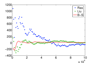
Figure 1: The lattice is a $(4,4)$ lattice and thus the adjacent matrix is $16\times 16$. The x-axis denotes the number of samplings and the y-axis denotes the error of the approximate cardinal number of configuration space.

According to the law of large numbers, the mean value of these samples gives an approximation to the permanent. But in fact, the number of samples in our computation is not really “large”. More precisely, a typical sample number in our computation would be $100,000$, while the cardinal number of the sample space could be, for example, $10^{115}$ (the two dimensional monomer-dimer model with $m=20$).

Notice that the probability distribution of the random variable $Y=\log X$ looks similar to the normal distribution. If the probability distribution of $Y$ is normal with $N(\mu,\sigma)$, then the expectation of $X$ would be

$$E(X)=E(e^{Y})=e^{\mu+\frac{\sigma^{2}}{2}}.$$

Other than computing the sample mean of $X$ directly, we can estimate the sample mean $\bar{\mu}$ and sample standard deviation $\bar{\sigma}$ of the random variable $Y$ first.

IV Experimental Results for Periodic Lattices

The algorithm SIS is used to approximate permanents, which gives approximation to the monomer-dimer constants. The algorithms are programmed in Matlab 7.0 and all computations in this paper run on Dell PC with CPU 2.8G Hz.

IV.1 Experiments on two dimensional lattices

Computational results for 2-dimensional monomer-dimer problems with periodic boundary conditions are presented in TABLE 2.

Table 2: $m$ denotes the size of the planar $(m,m)$ lattice. Every time, we sample $100,000$ samples and compute the approximate result of $logZ(m,2)/m^{2}$. We do this several times. SIS gives the median value of the approximate values; Time denotes the time in second for one sampling. A-PRE is the value given in BOS01

m	SIS	Time(sec)	A-PRE
4	0.663866	0.0012	0.6611
6	0.662851	0.0019	0.6629
8	0.662897	0.0028	0.6611
10	0.662951	0.0038	0.6663
12	0.662990	0.0055	0.6646
14	0.662852	0.0072	0.6638
16	0.662644	0.0100	—
18	0.663390	0.0138	—
20	0.662960	0.0181	—
22	0.663031	0.0237	—
24	0.662893	0.0307	—
26	0.663754	0.0398	—
28	0.663013	0.0507	—
30	0.663062	0.0710	—
32	0.662587	0.0769	—

Let compare with the results and the algorithm A-PRE, a Markov Chain Monte Carlo method used by Beichl, O’Leary, and SullivanBOS01 . Though computers used here are different, one can still tell the trends in the running times. The curve fitting results for algorithms SIS and A-PRE are shown in FIG 2. It is clear that the running times for both SIS and A-PRE grow polynomially with respect to $m$. The time complexity of SIS, the method developed in this paper, is about $O(m^{3})$ for 2-dimensional lattice, while the A-PRE, the MCMC method by BOS01 , is about $O(m^{5})$. Hence it is easy to tell that the algorithm SIS is faster distinctly. This suggests that the method SIS can be applied to large monomer-dimer problems.

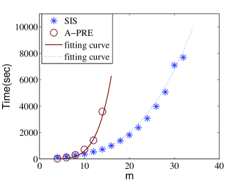
Figure 2: The relations between the running time of A-PRE method and SIS method with the lattice size $m$ are shown. The times of SIS method are costs of $100,000$ samples, those of A-PRE method are taken from BOS01 .

In order to fit the limit of $logZ(m,2)/m^{2}$ as $m$ goes to infinity, we apply regression to the computed mean values. The regression function is the same as BS99

$$y=\frac{p_{1}}{x^{2}}+p_{2},$$ (8)

where $x$ denotes the lattice size $m$, $y$ denotes the $h_{2}(m)$ and $p_{2}$ is the monomer-dimer constant. The monomer-dimer constant of 2-dimensional problem with periodic boundary can be obtained from the regression

$$h_{2}=0.6627\pm 0.0002\ \ with\ \ 95\%\ \ confidence.$$

The approximate results of the monomer-dimer constant coincides with the value $h_{2}=0.662798972834$ by Kong06 very well.

IV.2 Experiments on three dimensional lattices

For 3-dimensional problem with periodic condition, computational results are shown in TABLE 3. The time complexity for algorithm SIS in 3 dimensional problems is about $O(m^{6})$.

Table 3: $m$ denotes the size of the cubic $(m,m,m)$ lattice. Every time, we sample $100,000$ samples and compute the approximate result of $logZ(m,3)/m^{3}$. We do this several times. SIS gives the median value of the approximate values; Time denotes the time in second for one sampling. A-PRE is the value given in BOS01

m	SIS	Time(sec)	A-PRE
4	0.787359	0.0039	0.7844
6	0.786661	0.0082	0.7847
8	0.785821	0.0345	0.7870
10	0.787093	0.0919	—
12	0.785054	0.2483	—
14	0.783476	0.6693	—

To fit the limit of $logZ(m,3)/m^{3}$ as $m$ goes to infinity, we apply regression again. The function we use is

$$y=\frac{p_{1}}{x}+p_{2},$$ (9)

where $x$ denotes the lattice size $m$, $y$ denotes the $h_{3}(m)$ and $p_{2}$ is the monomer-dimer constant. The result is

$$h_{3}=0.7847\pm 0.0014\ \ with\ \ 95\%\ \ confidence.$$

This agrees well with the best known bound $0.7653\leq h_{3}\leq 0.7862$ FP05 .

V Discussions and Comments

The construction of the auxiliary bipartite graph is the key step in our formulation. Hence the permanent of the matrix $B$ in (4) gives the total number of matchings in the original bipartite graph $G(A)$. The size of the matrix $B$ doubles that of $A$. However since the special structure of the matrix $B$ can be explored in the algorithm, the computational cost does not really increase.

The Monte Carlo method we used in this paper is based on the sequential importance sampling. Each time one samples a term from the large sum defined by (2), and only nonzero terms are valuable in the computation. The formulation and computational methods that we propose in this paper never meet any zero term. This fact is not obvious but crucial for the efficiency of the algorithm. A rigorous mathematical proof will be presented elsewhere.

The regression function (8) for two dimensional is discussed and used by many authors, for example BS99 . It is based on asymptotic analysis. However (9) for three dimensional is just a result of statistical experiments. We are unable to give it any physical reasoning.

The basic contribution of this paper is the formulation and computational methods for approximating the number of all matchings in bipartite graphs. In this way, larger monomer-dimer systems can be studied.

- (1) O.J., Heilmann and E. H., Lieb, Commun. Math. Phys. 25, 190 (1972).
- (2) C. Kenyon, D. Randall, and A. Sinclair, J. Stat. Phys. 83, 637 (1996)
- (3) J.K., Roberts, Proc. Roy. Soc. (Landon) A 152, 464 (1935).
- (4) E.A. Guggenheim, Mixtures, (Clarendon Press, Oxford, 1952).
- (5) E.G.D. Cohen, J. de Boer, Z.W. Salsburg, Physica 11, 137 (1955).
- (6) J. Hammersley, in Research Papers in Statistics: Festschrift for J.Neyman, edited by F.David, (Wiley, London, 1966), p.125.
- (7) R.J. Baxter, J. Math. Phys. 9, 650 (1968).
- (8) D.S.Gaunt, Phys. Rev. 179, 174 (1969).
- (9) J. Hammersley, V. Menon, J. Inst. Math. Appl. 6, 341 (1970).
- (10) M.R. Jerrum, J. Stat. Phys. 48, 121 (1987).
- (11) I.Beichl, D.P.O’Leary, F.Sullivan, Phys. Rev. E 64, 016701 (2001).
- (12) S. Friedland and U.N. Peled, Adv. Appl. Math. 34, 486 (2005).
- (13) Y. Kong, Phys. Rev. E 74, 061102 (2006).
- (14) H.Minc, Permanents, (Encyclopedia Math. Appl. 6, 1978).
- (15) L.Lovasz, M.Plummer, Matching Theory, (Ann. of Discrete Math. 29, North-Holland, New York, 1986).
- (16) L.Valliant, Theoret. Comput. Sci. 8, 189 (1979).
- (17) N.Karmarkar, R.M.Karp, R.Lipton, L.Lovasz, M.Luby, SIAM J. Comput. 22, 284 (1993).
- (18) S.Chien, L.Rasmussen, A.Sinclair, J. Comput. System Sci. 67, 263 (2003).
- (19) M.Jerrum, A.Sinclair, E.Vigoda, Theoret. Comput. Sci. 51, 671 (2004).
- (20) J. Liu, Monte Carlo Strategies in Scientific Computing, (Springer Verlag, New York, 2001).
- (21) S.Friedland and D.Levy Mathematical papers in honour of Eduardo Marques de S, Textos de Matemtica # 39, (Coimbra University, Portugal, 2006), p.61.
- (22) L. E. Rasmussen, Random Struct. Algorithms. 5, 349 (1994).
- (23) I. Beichl, F. Sullivan, J. Comput. Phys. 149, 128 (1999).