Self-organization of heterogeneous topology and symmetry breaking in networks with adaptive thresholds and rewiring

Abstract

We study an evolutionary algorithm that locally adapts thresholds and wiring in Random Threshold Networks, based on measurements of a dynamical order parameter. A control parameter $p$ determines the probability of threshold adaptations vs. link rewiring. For any $p<1$, we find spontaneous symmetry breaking into a new class of self-organized networks, characterized by a much higher average connectivity $\bar{K}_{evo}$ than networks without threshold adaptation ($p=1$). While $\bar{K}_{evo}$ and evolved out-degree distributions are independent from $p$ for $p<1$, in-degree distributions become broader when $p\to 1$, approaching a power-law. In this limit, time scale separation between threshold adaptions and rewiring also leads to strong correlations between thresholds and in-degree. Finally, evidence is presented that networks converge to self-organized criticality for large $N$.

Interaction networks in nature often exhibit highly inhomogeneous architectures. Examples are scale-free degree distributions in protein networks MaslovSneppen2002 and metabolic networks Jeong2000 , mostly accompanied by intricate second order regularities as, for example, community structure Girvan2002 . The emergence of these properties often is explained by means of intuitive topology-based models, e.g. preferential attachment Barabasi99 or node duplications Bebek2006 . Real networks, however, are characterized not only by an evolving topology, but also by evolution of function, conveniently abstracted in terms of dynamics, i.e. the flow of information or matter on these networks. So far, only few studies explicitly consider the more general case of co-evolution between network dynamics and -topology BornholSneppen98 ; BornholRohlf00 ; BornholRoehl2003 ; LiuBassler2006 .

One example is the question how networks may evolve topologies that optimize biologically relevant parameters, e.g. flexible adaptation with respect to changing environments, or insensitivity against random perturbations of topology or dynamics (robustness) Savageau71 . In this context, Kauffman introduced random Boolean networks (RBN) to study the dynamics of gene regulatory networks from a global perspective Kauffman69 ; Kauffman93 . It was shown that RBN undergo a order-disorder transition at a critical wiring density (connectivity) $K_{c}=2$ Kauffman69 ; Kauffman93 ; DerridaP86 ; SoleLuque95 ; similar results were established for random threshold networks (RTN), which constitute a sub-class of RBN Kuerten88 ; RohlfBornhol02 ; Rohlf07 . It has been postulated that evolution should drive dynamical networks towards this ’edge of chaos’ to optimize adaptive flexibility and robustness Kauffman69 ; Kauffman93 . However, no mechanism able to generate critically connected networks could be provided.

To address this problem, a RTN-based model was proposed, linking rewiring of network nodes to local measurements of a dynamical order parameter, e.g. the average activity (magnetization) BornholRohlf00 . It was shown that this simple, local adaptive mechanism leads to a global self-organized critical state in the limit of large system sizes $N$. Subsequently, this principle was generalized to networks of noisy neurons BornholRoehl2003 and to RBN with evolvable logical functions LiuBassler2006 . Interestingly, finite size networks in these models evolve a broadly distributed heterogeneous in-degree connectivity LiuBassler2006 ; RohlfBornhol04 . Still, these topological heterogeneities are smaller than those observed in real-world networks, presumably because dynamical elements were assumed to be homogeneous with respect to their dynamical behavior. While this assumption leads to elegant models, it is quite unrealistic, as it becomes apparent e.g. in the frequent occurrence of canalizing functions in gene regulatory networks, with strong impact on dynamics in RBN models Moreira05 . Considering the accumulating experimental evidence of both close-to criticality RamoeKesseliYli06 and heterogeneous architecture Tong2004 in real gene regulatory networks, it is fascinating to speculate about a mechanism that might explain both observations: evolution of local dynamical heterogeneity and global homeostasis.

For this purpose, we introduce a minimal model linking regulation of activation thresholds and rewiring of network nodes in RTN to local measurements of a dynamical order parameter. A new control parameter $p\in[0,1]$ determines the probability of rewiring vs. threshold adaptations. We show that the symmetry of the evolutionary attractor for $p=1$ (no threshold adaptations, rewiring only) is broken spontaneously for any $p<1$. This new universality class of self-organized networks exhibits a much higher average connectivity $\bar{K}_{evo}$, compared to $p=1$ networks, however, with a value $\bar{K}_{evo}$ that is insensitive to $p$. In-degree distributions become very broad, approaching a flat power-law tail $\sim k_{in}^{-3/4}$ for $p\to 1$. Further, we establish the emergence of strong correlations between in-degree and thresholds in this limit, while for small $p$, correlations are weak. This indicates that an adaptive time-scale separation, with rare events of dynamical diversification and frequent rewiring, can lead to emergence of highly inhomogeneous topologies, without the need for network growth (as, for example, in preferential attachment models). Finally, we present evidence that networks with $p<1$ converge to a critical state for large $N$, however, with a finite size scaling significantly different from the one found for the case $p=1$.

Dynamics. We consider a network of $N$ randomly interconnected binary elements with states $\sigma_{i}=\pm 1$. For each site $i$, its state at time $t+1$ is a function of the inputs it receives from other elements at time $t$ (synchronous updates):

$$\sigma_{i}(t+1)=\begin{cases}+1&\text{if }f_{i}(t)>0\\ -1&\text{else}\end{cases}$$ (1)

with

$$f_{i}(t)=\sum_{j=1}^{N}c_{ij}\sigma_{j}(t)+h_{i}.$$ (2)

The interaction weights $c_{ij}$ take discrete values $c_{ij}=\pm 1$, with $c_{ij}=0$ if site $i$ does not receive any input from element $j$. Thresholds $h_{i}$ may vary from node to node, taking integer values $h_{i}\leq 0$ . In the following discussion, adaptive changes will be applied to the absolute value $|h_{i}|$, keeping in mind that the sign of $h_{i}$ is always negative.

As a dynamical order parameter, we define the average activity $A(i)$ of a site $i$

$$A(i)=\frac{1}{T_{2}-T_{1}}\sum_{t=T_{1}}^{T_{2}}\sigma_{i}(t).$$ (3)

Notice that a frozen site, i.e. a site that does not change its state, has $|A(i)|=1$, whereas an active site has $|A(i)|<1$.

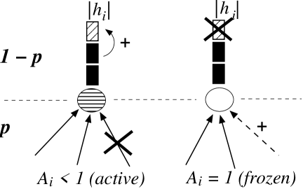
Figure 1: Left: with probability $p$, active nodes loose one of their inputs, with probability $1-p$ they increase their (absolute) threshold $|h_{i}|$. Right: frozen nodes show the opposite behavior.

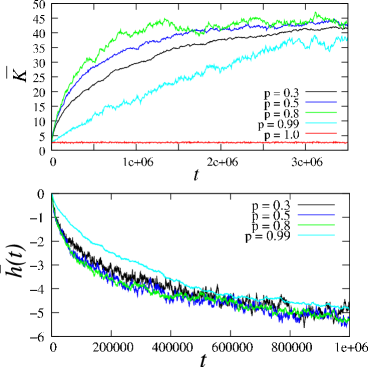
Figure 2: Upper panel: Evolution of the average connectivity $\bar{K}$ of threshold networks, using the adaptive algorithm (cf. Fig. 1), for $N=512$ and initial connectivity $\bar{K}_{ini}=1$. Time series for five different values of $p$ are shown. Lower panel: The same for the average threshold $\bar{h}$.

Figure 3: Upper four curves: Evolutionary mean values $\bar{K}_{evo}$ of the average connectivity, as a function of $p$; system sizes from top to bottom: $N=512$, $N=256$, $N=128$ and $N=64$. Lower four curves: The same for the evolutionary mean values $|\bar{h}_{evo}|$of the average absolute threshold. Statistics was taken over $10^{6}$ evolutionary steps, after a transient of $4\cdot 10^{6}$ steps.

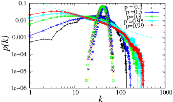
Figure 4: Line-pointed curves: in-degree distributions of evolved networks, data points only: the corresponding out-degree distributions (($\triangle$) $p=0.3$, (+) $p=0.5$, (x) $p=0.8$, (*) $p=0.95$, ($\square$) $p=0.99$). Statistics was gathered over $10^{6}$ evolutionary steps, after a transient of $4\cdot 10^{6}$ steps. Networks had size $N=512$. The dashed line has slope $-3/4$.

Figure 5: Average number $\langle k_{in}\rangle$ of inputs for a given node in evolving networks, as a function of the respective nodes (absolute) threshold $|h|$. Statistics was taken over $10^{6}$ rewiring steps, after a transient of $4\cdot 10^{6}$ steps. For all values $p<1$, a clear positive correlation between $\bar{k}_{in}$ and $|h|$ is found.

Figure 6: Average fraction $\bar{y}(N)$ of damaged nodes, 200 updates after a one-bit perturbation at time $t=0$, for different $p$, as a function of system size $N$. The lined curve is a fit of the average scaling behavior.

Topology evolution. Let us now discuss a particular evolutionary scheme that couples local adaptations of both the number of inputs and of thresholds to a site’s average activity. Analyzing Eq. (1) and Eq. (2), we realize that the activity of a site $i$ can be controlled in two ways: if $i$ is frozen, it can increase the probability to change its state by either increasing its number of inputs $k_{i}\rightarrow k_{i}+1$, or by making its threshold $h_{i}\leq 0$ less negative, i.e. $|h_{i}|\rightarrow|h_{i}|-1$. If $i$ is active, it can reduce its activity by adapting either $k_{i}\rightarrow k_{i}-1$ or $|h_{i}|\rightarrow|h_{i}|+1$. This adaptive scheme is realized in the following algorithm (see also Fig. 1):
1. Create a random network with average connectivity $\bar{K}_{ini}>0$ and average threshold $\bar{h}_{ini}=0$.
2. Select a random initial state $\vec{\sigma}_{ini}=(\sigma_{1},...,\sigma_{N})$.
3. Iterate network dynamics for $T$ timesteps.
4. Select a network site $i$ at random and measure its average activity $A_{i}$ over the last $T/2$ updates.
5. Adapt $k_{i}$ and $h_{i}$ in the following way:
- If $|A_{i}|<1$, then $k_{i}\rightarrow k_{i}-1$ with probability $p$ (removal of one randomly selected input). With probability $1-p$, adapt $|h_{i}|\rightarrow|h_{i}|+1$ instead.
- If $|A_{i}|=1$, then $k_{i}\rightarrow k_{i}+1$ with probability $p$ (addition of a new input from a randomly selected site). With probability $1-p$, adapt $|h_{i}|\rightarrow|h_{i}|-1$ instead. If $h_{i}=0$, let its value unchanged.
6. Go back to step 3.

If the control parameter $p$ takes values $p>1/2$, rewiring of nodes is favored, whereas for $p<1/2$ threshold adaptations are more likely. Notice that the model introduced in BornholRohlf00 is contained as the limiting case $p=1$ (rewiring only and $h_{i}=const.=0$ for all sites).

Results. After a large number of adaptive cycles, networks self-organize into a global evolutionary steady state. An example is shown in Figure 2 for networks with $N=512$: starting from an initial value $\bar{K}_{ini}=1$, the networks’ average connectivity $\bar{K}$ first increases, and then saturates around a stationary mean value $\bar{K}_{evo}$; similar observations are made for the average threshold $\bar{h}$ (Fig. 2, lower panel). The non-equilibrium nature of the system manifests itself in limited fluctuations of both $\bar{K}$ and $\bar{h}$ around $\bar{K}_{evo}$ and $\bar{h}_{evo}$. Regarding the dependence of $\bar{K}$ with respect to $p$, we make the interesting observation that it changes non-monotonically. Two cases can be distinguished: when $p=1$, $\bar{K}$ stabilizes at a very sparse mean value $\bar{K}_{evo}$, e.g. for $N=512$ at $\bar{K}_{evo}=2.664\pm 0.005$. When $p<1$, the symmetry of this evolutionary steady state is broken. Now, $\bar{K}$ converges to a much higher mean value $\bar{K}_{evo}\approx 43.5\pm 0.3$ (for $N=512$), however, the particular value which is finally reached is independent of $p$. The latter observation is made rigorous from measurements of $\bar{K}_{evo}$ for different $N$ over $10^{6}$ evolutionary steps, after systems have reached the steady state. While $\bar{K}_{evo}$ obviously depends on the system size $N$, curves are very flat with respect to $p$ (Fig. 3, upper four curves); the same holds for $|\bar{h}_{evo}|$ (Fig. 3, lower four curves). On the other hand, convergence times $T_{con}$ needed to reach the steady state are strongly influenced by $p$: $T_{con}(p)$ diverges when $p$ approaches $1$ (compare Fig. 2 for $p=0.99$). We conclude that $p$ determines the adaptive time scale. This is also reflected by the stationary in-degree distributions $p(k_{in})$ that vary considerably with $p$ (Fig. 4); when $p\to 1$, these distributions become very broad. The numerical data suggest that a power law

$$\lim_{p\to 1}p(k_{in})\propto k_{in}^{-\gamma}$$ (4)

with $\gamma\approx 3/4\pm 0.03$ is approached in this limit (cf. Fig. 4, dashed line). At the same time, it is interesting to notice that the evolved out-degree distributions are much narrower and completely insensitive to $p$ (Fig. 4, data points without lines).

How can one understand the emergence of broad in-degree distributions for with increasing $p$? Evidently, life times of both low thresholds $|h_{i}|\approx 0$ and high thresholds $|h_{i}|\gg 0$ become long for $p\to 1$. Since sites with low thresholds tend to be active and hence, on average, loose links, while sites with high thresholds tend to freeze and hence, on average, aquire new links, we would indeed expect that $p(k_{in})$ is broadened for $p\to 1$. On the other hand, for $p\to 0$, frequent adaptive changes of thresholds prevent long sequences of both frozen or highly active states, and hence make emergence of strong local wiring heterogeneities less probable. If this idea is correct, we would expect that, in the limit $p\to 1$, the in-degree of sites should exhibit a strong positive correlation to their thresholds, while for $p\to 0$ these correlations should be less pronounced. This is indeed exactly what we observe. For $p=0.99$, the average in-degree $\langle k_{in}\rangle$ of a given node, as a function of its threshold $|h|$, shows a steep increase, while the corresponding curve is relatively flat for $p=0.3$ (Fig. 5).

An interesting question is whether the networks with $p<1$ still approach a self-organized critical state for large $N$, as it was found for the case $p=1$ BornholRohlf00 . Since networks now evolve more densely wired, non-trivial topologies, this question has to be answered by application of a dynamical criterion. For this purpose, we studied damage spreading: after each adaptive step, dynamics was run from an initial system state $\vec{\sigma}$ and again from a direct neighbor state $\vec{\sigma}^{\,\prime}$ differing in one bit; after $t=200$ updates, the Hamming distance $d$ between both trajectories was measured and the average fraction of damaged nodes $\bar{y}(t)=:d/N$ was determined. Figure 6 shows $\bar{y}$, averaged over $10^{6}$ evolutionary steps, as a function of $N$. We find that the finite networks investigated here are all supercritical, however, $\bar{y}$ decreases monotonically with $N$. The average scaling behavior can be fit by

$$y(N)\approx a\cdot[\ln(N)]^{-\beta}$$ (5)

with $a=0.77\pm 0.02$ and $\beta=0.917\pm 0.01$. This dependence indicates that $\bar{y}=0$, i.e. the critical transition form chaotic to frozen dynamics, is approached for large $N$. Notice, however, that convergence is logarithmic, whereas for $p=1$ power laws were found BornholRohlf00 ; LiuBassler2006 . Again, this indicates that $p<1$ networks constitute an entirely new universality class.

To summarize, we studied a model of network evolution that couples both rewiring of inputs and adaptation of activation thresholds to local measurements of a dynamical order parameter. A control parameter $p$ determines the probability of threshold adaptations vs. link rewiring. While for $p=1$ (rewiring only, no threshold adapttation) networks evolve a self-organized critical state with a sparse average connectivity $\bar{K}_{evo}\approx 2$, for any $p<1$ (both rewiring and threshold adaptation) networks evolve a significantly more dense wiring, with broad heterogeneous in-degree distributions approaching a power-law $\sim k_{in}^{-3/4}$ for $p\to 1$. In this limit, time scale separation between rare threshold adaptations and frequent rewiring leads to emergence of strong correlations between thresholds and in-degree. We presented evidence that, in the limit of large $N$, networks logarithmically approach a self-organized critical state.

Our model presents a novel mechanism leading to co-evolution of topological and dynamical heterogeneity with robust homeostatic regulation, the latter reflected e.g. by the insensitivity of the evolved average connectivity with respect to $p$. Since similar - seemingly contradicting - observations are also made in experimental data of, e.g., gene regulatory networks RamoeKesseliYli06 ; Tong2004 , it is interesting to speculate that similar mechanisms might be at work in the evolution of biological networks.

References

- (1) S. Maslov and K. Sneppen, Science 296, 910 (2002)
- (2) H. Jeong et al., Nature 407, 651 (2000)
- (3) M. Girvan and M. E. J. Newman, Proc. Natl. Acad. Sci. USA 99, 7821 (2002)
- (4) A. L. Barabási and R. Albert, Science 286, 509 (1999)
- (5) G. Bebek et al., Theor. Comp. Sci 369, 239
- (6) S. Bornholdt and K. Sneppen, Phys. Rev. Lett. 81, 236 (1998)
- (7) S. Bornholdt and T. Rohlf, Phys. Rev. Lett. 84, 6114 (2000)
- (8) S. Bornholdt and T. Röhl, Phys. Rev. E 67, 066118 (2003)
- (9) M. Liu and K.E. Bassler, Phys. Rev. E 74, 041910 (2006)
- (10) M. A. Savageau, Nature 229, 542 (1971)
- (11) S.A. Kauffman, J. Theor. Biol. 22, 437 (1969)
- (12) S.A. Kauffman, The Origins of Order: Self-Organization and Selection in Evolution, Oxford University Press, 1993.
- (13) B. Derrida and Y. Pomeau, Europhys. Lett. 1, 45 (1986) 45
- (14) R. Solé and B. Luque, Phys. Lett. A 196, 331 (1995); B. Luque and R. Solé, Phys. Rev. E 55, 257 (1997)
- (15) K.E. Kürten, Phys. Lett. A 129, 157 (1988); K.E. Kürten, J. Phys. A 21, L615 (1988)
- (16) T. Rohlf and S. Bornholdt, Physica A 310, 245 (2002).
- (17) T. Rohlf, arxiv.org/abs/0707.3621 (2007)
- (18) T. Rohlf and S. Bornholdt, in: Function and regulation of cellular systems: experiments and models, ed. A. Deutsch, J. Howard, M. Falcke and W. Zimmermann; Birkhäuser Basel, p. 233-239 (2004)
- (19) A. A. Moreira and L. A. N. Amaral, Phys. Rev. Lett. 94, 218702 (2005)
- (20) P. Ramö, J. Kesseli and O. Yli-Harja, J. Theor. Biol. 242, 164 (2006)
- (21) A. H. Y. Tong et al., Science 303, 808 (2004)