Unbalanced Renormalization of Tunneling
in MOSFET-type Structures in Strong High-Frequency Electric Fields

Abstract

Two-dimensional electron gas coupled to adjacent impurity sites in high-frequency out-of-plane ac control electric field is investigated. Modification of tunneling rates as a function of the field amplitude is calculated. Nonlinear dependence on the ac field strength is reported for the conductivity of two-dimensional electron gas. It develops a periodic peak structure.

I Introduction

Rapid development of experimental techniques at nanoscaleJiang ; Jiang2 ; Craig ; Elzerman ; Koppens has stimulated theoretical advances in describing quantum phenomena for various geometries and settings. Extensive study has been done on nonlinear effects in a few state quantum system subject to strong harmonic control,DunlapKenkre ; GrossmannDittrich ; GrossmannHanggi ; DakhnovskiiBavli ; BavliMetiu ; HolthausHone ; RaghavanKenkre ; HanggiReview ; Burdov1 ; Burdov2 ; BurdovSolenov1 ; BurdovSolenov2 ; BurdovSolenov3 ; Romanovs such as a double quantum dot,BurdovSolenov2 an array of coupled quantum dots,BurdovSolenov3 superlatices,Romanovs etc. In this paper, we investigate the influence of the ac field on one-state quantum objects coupled to two-dimensional electron gas (2DEG) via tunneling.

The systems of such geometry have been recently used in experimental as well as theoretical study of few and single electron spin manipulations,Koppens spin-to-charge conversion measurements,Elzerman Ruderman-Kittel-Kasuya-Yosida (RKKY),Craig and quantum HallLewis effects. In the mentioned experiments, 2DEG is formed by confinement in a two-dimensional layer grown in a pile between between the layers of the wide gap material. The electron concentration in 2DEG can be varied significantly and is usually controlled electrostatically by split-gate technique. A similar system can be also created in the inversion layer in metal oxide semiconductor field effect transistors (MOSFETs). In both cases, the impurity centers (sites), localized usually outside the 2DEG in adjacent layers, play an important role.Ralls ; Mozyrsky One of the first experimental evidences here was the observation of random telegraph noise in conduction of the inversion layer in MOSFET.Ralls

Surprisingly, little attention has been given to the control of the impurity states, and thus the properties of 2DEG, dynamically. Unlike the well-known phenomena of dynamical control of tunnelingHanggiReview ; Burdov1 ; Burdov2 ; BurdovSolenov1 ; BurdovSolenov2 ; BurdovSolenov3 in few state electron systems, e.g., double quantum dot, the impurity-2DEG system provides more degrees of freedom to change properties and correlations which are not related to tunneling directly. One of the examples here is the possible indirect influence over the RKKY interaction mediated by 2DEG electrons.Craig

In what follows, we demonstrate that periodic high frequency potential (electric field) applied perpendicular to 2DEG leads to nontrivial renormalization and disbalance of the tunneling between the impurity sites and 2DEG. Moreover, tunneling modification, as well as Coulomb activation of the impurity sites, induces oscillatory behavior of 2DEG conductivity as a function of the amplitude of applied periodic field. This variation is similar to Shubnikov–de Haas oscillationsEngel but have different underlying physics.

In the next section, we formulate the impurity-2DEG model. Section III is devoted to the construction of the corresponding stationary many-body problem using Floquet states. Time-averaged quantities of interest are defined. In Secs. IV and V, nonlinear dependence of tunneling rates is obtained, starting with the simpler case that neglects 2DEG electron scattering on impurity. The scattering dynamics is analyzed. Finally, in Sec. VI, field amplitude dependence of conductivity is found. This dependence, together with the expression of the tunneling rates, is the main result of the paper.

II Model

As mentioned above, we consider zero temperature 2DEG interacting with an impurity electron localized in the adjacent layer of a wide gap material. Both systems are subject to external plane polarized harmonic field, $E_{z}(t)$, with the frequency $\omega_{0}$ and polarization along $z$ axis, perpendicular to the 2DEG plane, see Fig. 1. The field is treated in the dipole approximation appropriate as soon as the characteristic size of the nanostructure is smaller compared to the field wavelength. The impurity-2DEG interaction is via tunneling between 2DEG and impurity states, as well as through Coulomb scattering of conduction electrons on empty, positively charged, donor impurity site. The electrons are considered spinless, and only the ground state of the impurity site is taken into account. In many cases, the heterostructure has more than one impurity site next to the conduction layer. This situation, including the effect of spins, is discussed in the last sections, and in most cases, the effect of the external field can be deduced from the one-site spinless model investigated below.

The unperturbed Hamiltonian is

$$H_{0,i}=\frac{p_{i}^{2}}{2m}+U_{d}(\mathbf{r}_{i})\delta_{i,d}+U_{\textrm{2DEG}}(z_{i})\delta_{i,\mathrm{2DEG}},$$ (2.1)

where $U_{d}(\mathbf{r})$ is the impurity localization potential, and $U_{\textrm{2DEG}}(z)$ denotes the potential profile that forms 2DEG. The $\delta$ functions are defined so that $H_{0,i}$ resemble the unperturbed Hamiltonian of an electron sitting on the impurity ($\delta_{i,d}=1$, $\delta_{i,\mathrm{2DEG}}=0$) and in the 2DEG ($\delta_{i,d}=0$, $\delta_{i,\mathrm{2DEG}}=1$). The interaction between electrons as well as due to the external field is

$$V=-eE_{z}(t)\sum\limits_{i}{z_{i}}+\sum\limits_{j\neq i}\frac{e^{2}}{4\pi\epsilon_{0}\epsilon}\frac{e^{-q_{s}|{\bf{r}}_{i}-{\bf{r}}_{j}|}}{|{\bf{r}}_{i}-{\bf{r}}_{j}|},$$ (2.2)

where $E_{z}(t)=E_{z}\cos\omega_{0}t$, and $q_{s}$ represents the screening wave vector. Following the standard procedure, we define the amplitudes

$$H_{k0}^{*}=H_{0k}=\int{d{\bf{r}}}\psi_{0}^{*}({\bf{r}})\left[H_{0,i}-\frac{p_{i}^{2}}{2m}\right]\psi_{k}({\bf{r}})$$ (2.3)

and

$$V_{kk^{\prime}} = -2\int d\mathbf{r}d\mathbf{r}^{\prime}|\psi_{0}({\bf{r}})|^{2}$$

$$\times \psi_{k}^{*}({\bf{r}}^{\prime})\psi_{k^{\prime}}({\bf{r}}^{\prime})\frac{e^{2}}{{4\pi\epsilon_{0}\epsilon}}\frac{{e^{-q_{s}\left|{{\bf{r}}-{\bf{r}}^{\prime}}\right|}}}{{\left|{{\bf{r}}-{\bf{r}}^{\prime}}\right|}}.$$

Here, $\psi_{0}({\bf{r}})$ is the wave function of the noninteracting ground state localized on the impurity, i.e., $H_{0,d}\psi_{0}({\bf{r}})=E_{0}\psi_{0}({\bf{r}})$, and $\psi_{k}({\bf{r}})$ corresponds to the $k$-th state in 2DEG, i.e., $H_{0,\mathrm{2DEG}}\psi_{k}({\bf{r}})=E_{k}\psi_{k}({\bf{r}})$. The shape of $\psi_{0}({\bf{r}})$ and $\psi_{k}({\bf{r}})$ depends on the form of $U_{d}({\bf{r}})$ and $U_{\mathrm{2DEG}}({\bf{r}})$. Though it is not, strictly speaking, necessary, we will assume $H_{0k}$ to be independent of $k$ and real, i.e., $H_{k0}^{*}=H_{0k}\to\Delta$, to simplify notations. The electron-electron interaction in 2DEG is ignored. With the above notations, we arrive to the Hamiltonian

$$H = \left[{E_{0}+V_{00}(t)}\right]d^{\dagger}d+\sum\limits_{k}{\left[{E_{k}+V_{2DEG}(t)}\right]}c_{k}^{\dagger}c_{k}$$ (2.5)

$$+ dd^{\dagger}\sum\limits_{kk^{\prime}}{V_{kk^{\prime}}}c_{k}^{\dagger}c_{k^{\prime}}+\Delta\sum\limits_{k}{\left({d^{\dagger}c_{k}+c_{k}^{\dagger}d}\right)},$$

where $V_{00}(t)=-eE_{z}(t)\int d\mathbf{r}\psi_{0}^{*}({\bf{r}})z\psi_{0}({\bf{r}})$ and, similarly, $V_{\textrm{2DEG}}(t)\sim\int d\mathbf{r}\psi_{k}^{*}({\bf{r}})z\psi_{k}({\bf{r}})$. The latter is assumed to be independent of $k$ since only the distribution along $z$ of the lowest band is of interest. The $z$ distribution of $|\psi_{0}({\bf{r}})|^{2}$ and $|\psi_{k}({\bf{r}})|^{2}$ is concentrated around, respectively, the impurity center and the middle of the $U_{\mathrm{2DEG}}$ quantum well. Therefore, $z_{0,0}=\int d\mathbf{r}\psi_{0}^{*}({\bf{r}})z\psi_{0}({\bf{r}})$ and $z_{k,k}=\int d\mathbf{r}\psi_{k}^{*}({\bf{r}})z\psi_{k}({\bf{r}})$ refer to the position of the impurity and 2DEG along the $z$ axis. As we will see later, only the difference between these two quantities is of interest.

One can adopt the following values for order of magnitude estimates. With the separation between the impurity and 2DEG of the order of several angstroms, and the barrier height of the order of several eV, the tunneling amplitude will vary by $\sim 1\div 10$ meV and smaller depending on the distance. The frequency $\omega_{0}$ is of the order $\sim 10$ meV; the temperatures $T\lesssim 1$ K; the size quantization $\gtrsim 100$ meV. These values are feasible for Si/SiO₂ structures.

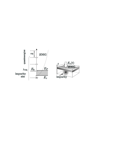
Figure 1: Impurity site coupled to the 2DEG conduction electrons. Strong ac field of frequency $\omega_{0}$ is applied perpendicular to 2DEG. The ladder of quasienergies develops. All quasienergies above $E_{F}$ and within the range of $\sim\lambda\omega_{0}$ are used for tunneling out process. The quasienergies below the bottom of the conduction band, $E_{c}$, are not active.

III Floquet States

The Hamiltonian (2.5) is periodic in time with the period $2\pi/\omega_{0}$. It is natural to utilize this symmetry.Shirley ; Zeldovich ; Ritus Similar to space-periodic solid state lattice structures, it was shownZeldovich that the wave function corresponding to the periodic Hamiltonian is of the form

$${|\psi_{\varepsilon}(t)\rangle}=e^{-i\varepsilon t}{|u^{\varepsilon}(t)\rangle},$$ (3.1)

where ${|u^{\varepsilon}(t)\rangle}={|u^{\varepsilon}(t+2\pi/\omega_{0})\rangle}$, and $\varepsilon$ is the quasienergy. Moreover, it was demonstrated that the set of quasienergy states can be treated similarly to the conventional system of stationary eigenstates—i.e., the system initially set up in a certain quasienergy state (or distribution over these states) remains at the same state (or with the same distribution) over the entire evolution of the system.Zeldovich

The transitions between the quasienergy states correspond to the perturbations which break the periodicity. This has been investigated in the literature.SolenovBurdov In our case, we assume the time scale of such perturbations due to environment (or other factors) to be much larger than the one of interest. As a result, one can analyze the quasienergy spectrum of the model to obtain the information about tunneling effects in the system.

Let us show a few steps to support the above statement. It is convenient to use the interaction representation, factoring out the evolution due to the oscillatory part of the Hamiltonian (2.5). The corresponding evolution operator, $U_{0}(t)=\exp\{\frac{i}{{\omega_{0}}}\sin\omega_{0}t[{V_{00}d^{\dagger}d+V_{2DEG}\sum_{k}{c_{k}^{{}^{\dagger}}c_{k}}}]\}$, is still periodic so that one can define

$${|\tilde{\psi}_{\varepsilon}(t)\rangle}=U_{0}^{\dagger}(t){|\psi_{\varepsilon}(t)\rangle}=e^{i\varepsilon t}{|\tilde{u}^{\varepsilon}(t)\rangle},$$ (3.2)

with ${|\tilde{u}^{\varepsilon}(t)\rangle}={|\tilde{u}^{\varepsilon}(t+2\pi/\omega_{0})\rangle}$. The corresponding Schrodinger equation is

$$i\frac{d}{{dt}}{|\tilde{\psi}_{\varepsilon}(t)\rangle}=H(t){|\tilde{\psi}_{\varepsilon}(t)\rangle},$$ (3.3)

where

$$H(t) = E_{0}d^{\dagger}d+\sum\limits_{k}E_{k}c_{k}^{\dagger}c_{k}+dd^{\dagger}\sum\limits_{kk^{\prime}}V_{kk^{\prime}}c_{k}^{\dagger}c_{k^{\prime}}$$ (3.4)

$$+ \Delta\sum\limits_{k}{\left({d^{\dagger}c_{k}e^{-i\lambda\sin\omega_{0}t}+c_{k}^{\dagger}de^{i\lambda\sin\omega_{0}t}}\right)}.$$

The effective strength of the external periodic field is defined as $\lambda=(V_{00}-V_{\textrm{2DEG}})/\omega_{0}$ with $V_{00}$ and $V_{\textrm{2DEG}}$ representing the amplitudes of $V_{00}(t)$ and $V_{\textrm{2DEG}}(t)$ respectively. Note that $V_{00}$ and $V_{\textrm{2DEG}}$ have opposite signs and, thus, $\lambda$ is proportional to the average distance $|z_{0,0}-z_{k,k}|$.

Our goal is to obtain the equation for quasienergy. One can easily form equations for the Fourier transform of the periodic part of the quasienergy wave function, ${|\tilde{u}^{\varepsilon}(t)\rangle}=\sum_{m}{e^{im\omega_{0}t}}{|\tilde{u}^{\varepsilon}_{m}\rangle}$. From Eq. (3.3) we have

$$\sum\limits_{m}{e^{-im\omega_{0}t}}\left[{\varepsilon+\omega m-H(t)}\right]{|\tilde{u}^{\varepsilon}_{-m}\rangle}=0.$$ (3.5)

Let us now recall that the time-dependent exponentials in Hamiltonian (3.4) have a simple series representation $e^{i\lambda\sin\omega t}=\sum_{n=-\infty}^{\infty}{J_{n}(\lambda)e^{in\omega_{0}t}}$ in terms of the Bessel functions. It should be noted that the harmonic form of the external field, and thus the time-dependent exponential in Eq. (3.4), is not necessary. For any periodic zero-average field, one can define the above series representation. In this case, the Bessel functions $J_{n}(\lambda)$ are replaced with the coefficients, $J_{n}(\lambda)\to f_{n}(\lambda)$, which carry the structure of a single oscillation. The results obtained below will be qualitatively the same with this modification. Since the harmonic field provides more insight into the physics of the phenomenon, we use it in further derivations instead of a more complicated time-periodic potential.

Defining a vector column of the states as ${|v\rangle}=\{...,{|\tilde{u}_{-1}\rangle},{|\tilde{u}_{0}\rangle},{|\tilde{u}_{1}\rangle},...\}^{T}$, we finally obtain the time-independent Schrodinger equation for quasienergies,

$${\bf{H}}{|v\rangle}=\varepsilon{|v\rangle},$$ (3.6)

where the stationary Hamiltonian is

$${\bf{H}} = E_{0}d^{\dagger}d+\sum\limits_{k}{E_{k}c_{k}^{{}^{\dagger}}c_{k}}+\omega_{0}I_{z}+dd^{\dagger}\sum\limits_{kk^{\prime}}V_{kk^{\prime}}{c_{k}^{\dagger}c_{k^{\prime}}}$$ (3.7)

$$+ \sum\limits_{n,k}{\Delta J_{n}(\lambda)\left({I_{-}^{(n)}c_{k}^{\dagger}d+I_{+}^{(n)}d^{\dagger}c_{k}}\right)}.$$

Here the additional operators are understood, if one defines a column vector, $|e_{m}\rangle$, with all entries zeros except for the $m$-th entry which is “1.” Then, $I_{z}|e_{m}\rangle=m|e_{m}\rangle$, $I_{\pm}|e_{m}\rangle=|e_{m\pm 1}\rangle$. We use the superscript in parentheses to generalize the power as $I_{\pm}^{(-n)}\mathop{=}\limits^{n>0}I_{\mp}^{(n)}\mathop{=}\limits^{n>0}I_{\mp}^{n}$. The quasienergy spectrum is now a solution to the Kondo-type spin-assisted tunneling problem, where operators $I_{\pm}$ correspond to renormalized rising (lowering) operators of a large integer spin ($S\to\infty$), or an asymptotically large ensemble of identical two-state systems. Note that $I_{\pm}$, as they have been introduced to rewrite Eq. (3.5) in the form (3.6), are not quite the spin rising (lowering) operators. Nevertheless, in the limit of large spin ($S\to\infty$) and finite magnetization, they differ only by a constant factor which has no effect on the subsequent calculations.spincomment

We should also demonstrate that the stationary problem with Hamiltonian (3.7) is sufficient to compute physically observable quantities of interest. In this paper, we are after the tunneling process in between the impurity and 2DEG, as well as the conductivity of 2DEG, therefore, it is natural to investigate the dynamics of the average occupation number for the impurity site, i.e., $\overline{\langle\psi(t)|dd^{\dagger}|\psi(t)\rangle}^{t}$, or the amplitude of 2DEG electron transitions for states $k,k^{\prime}$, i.e., $\overline{\langle\psi(t)|c_{k}c_{k^{\prime}}^{\dagger}|\psi(t)\rangle}^{t}$. The time-average is over the period $2\pi/\omega_{0}$ of the fast external field oscillations.

Taking into account the properties of the quasienergy states, we can focus on the average over a single quasienergy state. As mentioned above, the average of two conjugate operators of the same type is sought. This simplifies the expression further as $\langle\psi_{\epsilon}(t)|dd^{\dagger}|\psi_{\epsilon}(t)\rangle=\langle\tilde{\psi}_{\epsilon}(t)|dd^{\dagger}|\tilde{\psi}_{\epsilon}(t)\rangle$. The time-averaged quantity becomes

$$\overline{\langle\tilde{\psi}_{\epsilon}(t)|dd^{\dagger}|\tilde{\psi}_{\epsilon}(t)\rangle}^{\,t}=\sum_{m}\langle\tilde{u}_{m}|S(0,t)d(t)d^{\dagger}(t)S(t,0)|\tilde{u}_{m}\rangle$$ (3.8)

Here, the operators are in the interaction picture and evolve according to the first three (main) terms of the Hamiltonian (3.7), while the standard scattering matrix is due to the perturbation—the last two terms in Eq. (3.7).

As a result, the dynamics of the average occupation probability at the impurity site is entirely determined by time-independent Hamiltonian (3.7). Similar arguments hold for the transition amplitudes in 2DEG and thus the conductivity. A standard equilibrium procedure of switching the interaction “on” adiabatically from $t=-\infty$ can be used. In this case the initial dynamics is stationary in the first place, $|\tilde{\psi}_{\epsilon}(t)\rangle=\mathrm{const}$, since Hamiltonian (3.4) becomes time-independent. This makes $|\tilde{u}_{m}\rangle=|\tilde{u}_{0}\rangle\delta_{0,m}$. The expression for the average becomes

$$\overline{\langle\tilde{\psi}_{\epsilon}(t)|dd^{\dagger}|\tilde{\psi}_{\epsilon}(t)\rangle}^{\,t}=$$

$$= \langle\tilde{u}_{0},e_{0}|S(-\infty,t)d(t)d^{\dagger}(t)S(t,-\infty)|\tilde{u}_{0},e_{0}\rangle,$$

where $|\tilde{u}_{0}\rangle$ is the usual initial state for noninteracting fermions. In what follows, we will use the shorthand notation for the complete average $\langle S(-\infty,t)d(t)d^{\dagger}(t)S(t,-\infty)\rangle$ instead of the one in Eq. (III).

IV Nonlinear tunneling without scattering

In this section, we obtain the tunneling rates considering Hamiltonian (3.7) without Coulomb scattering on the impurity, i.e., the fourth term. Let us explicitly show the main part,

$${\bf{H}}_{0}=E_{0}d^{\dagger}d+\sum\limits_{k}{E_{k}c_{k}^{{}^{\dagger}}c_{k}}+\omega_{0}I_{z}$$ (4.1)

and the perturbation,

$$\mathbf{V}=\sum\limits_{n,k}{\Delta J_{n}(\lambda)\left({I_{-}^{(n)}c_{k}^{\dagger}d+I_{+}^{(n)}d^{\dagger}c_{k}}\right)}.$$ (4.2)

The perturbation (4.2) leads to equilibration of the impurity occupation probability $P$. Using this state for averaging, we have $\langle S(-\infty,\infty)\rangle=e^{i\phi}$. As a result, the tunneling rates can be found by calculating the zero-temperature impurity electron self-energy. The Green’s function $G(t,t^{\prime})=-i\langle Td(t)d^{\dagger}(t^{\prime})S(\infty,-\infty)\rangle$ is of interest, where $S(t_{2},t_{1})=T\exp[-i\int_{t_{1}}^{t_{2}}dt^{\prime}\mathbf{V}(t^{\prime})]$.

For small $\Delta$, one-loop approximation is sufficient.phonons In Appendix A, we calculate the self-energy for higher orders in $\Delta$. However, they do not introduce any new physics and may be omitted. The tunneling rate $\gamma$ is given by imaginary part of the self-energy,

$$\Sigma_{1}(\omega)=\sum\limits_{m,k}{\Delta^{2}}J_{m}^{2}(\lambda)g_{k}(\omega-m\omega_{0}),$$ (4.3)

where $g_{k}(\omega)$ is noninteracting Green’s function of 2DEG electrons. The tunneling in and out from the impurity can be clearly separated. The result is

$$\gamma_{in/out}=-2\pi\Delta^{2}D_{2}\sum\limits_{m=M^{1}_{in/out}}^{M^{2}_{in/out}}{J_{m}^{2}(\lambda)}.$$ (4.4)

Here, $D_{2}$ is the density of states for 2DEG. The limits are $M^{1}_{in}=-\theta(E_{0}-E_{F})$, $M^{2}_{in}=-\sum_{n=1}^{\omega_{0}/E_{F}}\theta(E_{0}-n\omega_{0}-E_{F})$, and $M^{1}_{out}=\theta(E_{F}-E_{0})+M^{2}_{in}$, $M^{2}_{out}=\infty$, where $E_{F}$ is the Fermi energy of 2DEG. These limits and the summation terms have a clear physical meaning. They correspond to tunneling in and out from the impurity quasienergy states, see Fig. 1. At the same time, they may be viewed in terms of allowed multiphoton processes from the 2DEG state below the Fermi surface (tunneling in, negative $m$) and to the empty states above $E_{F}$ (tunneling out, positive $m$). However, the latter language should be used keeping in mind the explanation via the quasienergies. The actual photons also account for the renormalization of the tunneling amplitude, which is done automatically in our treatment. The infinity in $M^{2}_{out}$ is true in the limit sense, ${\lim}_{E_{\infty}\gg\omega_{0}}E_{\infty}/\lambda\omega_{0}$, and denotes the upper edge, $E_{\infty}$, of the 2DEG band or the next conduction band if present relative to the external field strength $\lambda\omega_{0}$.

To be specific, let us discuss the case when the electron concentration in the conduction channel, $n_{0}$, is low, such that the Fermi energy of 2DEG (with respect to the bottom of the conduction band, $E_{c}$) is smaller as compared to the external field frequency. The magnitude of the field exceeds the latter and is much smaller than $E_{\infty}$. The chain inequality is $E_{0}\sim E_{F}<\omega_{0}\lesssim\omega_{0}\lambda\ll E_{\infty}$, where all the energies are measured from the bottom of the 2DEG conduction band, $E_{c}$. This is a natural assumption for many 2DEG systems used for few electron manipulation in recent experiments. The tunneling rates are

$$\gamma_{in}=-2\pi\Delta^{2}D_{2}J_{0}^{2}(\lambda)\theta(E_{F}-E_{0})$$ (4.5)

and

$$\gamma_{out}=-2\pi\Delta^{2}D_{2}\sum\limits_{m=\theta(E_{F}-E_{0})}^{\infty}{J_{m}^{2}(\lambda)}.$$ (4.6)

For a weak external harmonic field, $\lambda\ll 1$, both tunneling rates approach the well known result $\gamma_{0}=-2\pi\Delta^{2}D_{2}\theta(\pm E_{F}\mp E_{0})$. This is also true for the more general case given in Eq. (4.4). The low amplitude of the field suppresses the multiphoton absorption (emission) process, $J_{m>1}^{2}(\lambda)\to 0$, and allows the single photon processes as a small first-order correction, $J_{1}^{2}(\lambda)$, while the renormalization of the non-assisted tunneling vanishes, $J_{0}^{2}(\lambda)\to 1$.

Larger external field amplitudes activate more quasienergy states. Keeping in mind the earlier discussion, this process can also be viewed in terms of induction of multiphoton transitions with the maximal number of photons absorbed (emitted) per transition $\sim\lambda$. In this case, the tunneling rates depart from each other, see Fig. 2. In the limiting case of $\lambda\gg 1$, the tunneling out rate becomes $\gamma_{out}\to-2\pi\Delta^{2}D_{2}\frac{1}{2}$, while $\gamma_{in}$ oscillates according to $J^{2}_{0}(\lambda)$ and converges to zero as $\sim 1/\lambda$. Similar results can be obtained directly by averaging the transition matrix element due to Hamiltonian (2.5) over the fast oscillations of driving field, keeping the terms of the order $\Delta^{2}$, see Appendix B. The above approach, however, provides more physical insight and is more convenient for further discussion.

It should be noted that the above results apply in a more general case when $E_{0}$ is significantly higher or lower then $E_{F}$. In this case one can define $\bar{E}_{0}=E_{0}+\bar{m}\omega_{0}$, such that $|\bar{E}_{0}-E_{F}|<\omega_{0}$. Different quasienergy comes near the resonance with the Fermi surface, see Fig. 1. The same form of the expression for the tunneling rates, Eqs. (4.5) and (4.6), can be used by replacing $E_{0}\to\bar{E}_{0}$ and $J_{m}(\lambda)\to J_{m+\bar{m}}(\lambda)$.

V Scattering Dynamics

Let us now investigate the modification of tunneling rates due to scattering, i.e., the fourth term, $V_{sc}$, of the Hamiltonian (3.7), ignored in the previous section. This problem is similar to the problem of x-ray edge singularity.NozieresDominics To produce a tractable solution, one has to assume a special form of the scattering potential, $V_{kk^{\prime}}\to Vu_{k}u_{k^{\prime}}$. Here, $u_{k}$ is the cutoff function which is of the order ${\cal O}(1)$ for $E_{k}\sim E_{F},\lambda\omega_{0}$ and vanishes for $E_{k}\sim E_{\infty}$. We also assume $u_{k}$ to be symmetric.

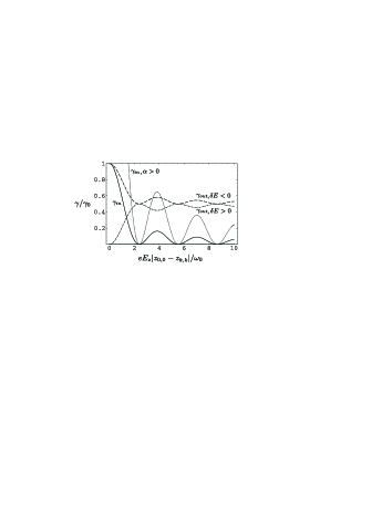
Figure 2: Tunneling rates as a function of harmonic field amplitude. The rates are given in terms of zero-field tunneling rate amplitude $\gamma_{0}$. The dotted curve represents the tunneling in rate with singular renormalization factor due to scattering with $\alpha>0$. In this case, only qualitative dependence is presented, since the scattering factor will involve regularization, as discussed in the text.

One can notice that the scattering is only present when the electron leaves the impurity site.NozieresDominics This differentiates the tunneling in and out processes. To investigate the two in a uniform treatment, it is convenientNozieresDominics to redefine the perturbation due to scattering for tunneling in as $V_{sc}=-Vd^{\dagger}d\sum_{kk^{\prime}}u_{k}u_{k^{\prime}}c_{k}^{\dagger}c_{k^{\prime}}$. We add the corresponding term to the unperturbed Hamiltonian, i.e., $\mathbf{H}_{0}\to\mathbf{H}_{0}+\sum_{kk^{\prime}}u_{k}u_{k^{\prime}}c_{k}^{\dagger}c_{k^{\prime}}$. This will only redefine the noninteracting conduction electron Green’s function, $\tilde{g}_{kk^{\prime}}(\omega)=g_{k}(\omega)\delta_{kk^{\prime}}-iV\sum_{k^{\prime\prime}}g_{k}(\omega)u_{k}u_{k^{\prime\prime}}\tilde{g}_{k^{\prime\prime}k^{\prime}}(\omega)$. For tunneling out, one still has $V_{sc}=Vdd^{\dagger}\sum_{kk^{\prime}}u_{k}u_{k^{\prime}}c_{k}^{\dagger}c_{k^{\prime}}$.

To utilize the results of Ref. NozieresDominics, , note that the tunneling rates can also be obtained by calculating the time derivative of $\langle Td(t)d(t\pm 0)S(\infty,-\infty)\rangle$. The expression correct up to $\Delta^{2}$ is

$$\gamma_{in/out}={\mathop{\rm Re}\nolimits}\sum\limits_{n,k}{\Delta^{2}J_{n}^{2}(\lambda)}$$

$$\times \int\limits_{-\infty}^{\infty}{dt^{\prime}}\langle|Tc_{k}^{\dagger}(t)d(t)d^{\dagger}(t^{\prime})c_{k}(t^{\prime})|\rangle\langle I_{-}^{(n)}(t)I_{+}^{(n)}(t^{\prime})\rangle.$$

Here, the state $|\rangle$ include the $|0\rangle$ or $|1\rangle$ state of the impurity for the tunneling in or out cases, respectively. The problem is to compute the average

$$F(t-t^{\prime})=\sum_{kk^{\prime}}{u_{k}u_{k^{\prime}}}\langle T\bar{c}_{k}^{\dagger}(t)\bar{d}(t)\bar{d}^{\dagger}(t^{\prime})\bar{c}_{k^{\prime}}(t^{\prime})\rangle.$$ (5.2)

Then, the rates are found from $F(t)$ via its Fourier transform as

$$\gamma_{in/out}={\mathop{\rm Re}\nolimits}\sum\limits_{n,k}{\Delta^{2}J_{n}^{2}(\lambda)}F(n\omega_{0}).$$ (5.3)

With the above redefinition of the scattering perturbation, the average (5.2) can be computed for any magnitude of the scattering amplitude as a one-body problem with time-dependent potential (scattering on impurity), as it was demonstrated by Nozieres and De Dominics.NozieresDominics This is possible since we assume that the impurity has no internal degrees of freedom. If one defines the times of two tunneling acts by $t$ and $t^{\prime}$, the average (5.2) is found via the time evolution of $\varphi_{kk^{\prime}}(\tau,\tau^{\prime},t,t^{\prime})=\langle T\bar{c}_{k}(\tau)\bar{c}_{k^{\prime}}^{\dagger}(\tau^{\prime})\rangle$ with all the vertices describing the scattering acts restrained to the interval $(t,t^{\prime})$. The overbar denotes complete evolution.

When the region around the Fermi energy is of interest, $|\delta E|\ll\omega_{0}$ and $m=0$, the asymptotic form of the scattering can be used.NozieresDominics This adds a singular factor to $F(\omega\to 0)$, and thus the tunneling rate, of the form

$$\left[{\xi_{0}}/{(\pm\delta E)}\right]^{\alpha},$$ (5.4)

where $\alpha=2\delta/\pi-(\delta/\pi)^{2}$ and $\delta E=E_{F}-E_{0}$. In two dimensions the phase shift is defined by $\tan\delta=\pi D_{2}V$. Here, $\xi_{0}$ is the cutoff coming from $u_{k}$. The exponent in Eq. (5.4) is found within logarithmic accuracy.

In our case, higher energy terms are present. They do not comply with the asymptotic approximation for the scattered wave functions used to obtain Eq. (5.4). For higher energies, $m\neq 0$, a short-time dynamics of $F(t)$ is necessary. In the case when $Vt\ll 1$, it is possible to omit the integral term in Eq. (35) of Ref. NozieresDominics, . In other words, the scattering becomes less important. As the result, the corresponding tunneling terms are the same as in the previous section up to ${\cal O}(V/m\omega_{0})$ corrections which are negligible provided $V/\omega_{0}\ll 1$. The tunneling due to large $V$ is also clear. The tail of the scattering renormalization will be added, as a factor, until approximately the $n\sim V/\omega_{0}$ tunneling term.

Finally, for the case of Eqs. (4.5) and (4.6) and assuming that $|\delta E|\ll\omega_{0}$, we obtain

$$\gamma_{in}=-2\pi\Delta^{2}D_{2}J_{0}^{2}(\lambda)\theta(\delta E)\left({\frac{{\xi_{0}}}{{\delta E}}}\right)^{\alpha}$$ (5.5)

and

$$\gamma_{out}= - 2\pi\Delta^{2}D_{2}J_{0}^{2}(\lambda)\theta(-\delta E)\left(\frac{\xi_{0}}{-\delta E}\right)^{\alpha}$$

$$- 2\pi\Delta^{2}D_{2}\sum_{m=1}^{\infty}J_{m}^{2}(\lambda).$$

When the external harmonic field is weak the tunneling rates again approach the standard expression (with the scattering renormalization). For strong fields, the result depends on the scattering exponent as well as on $\delta E$, unlike in Eqs. (4.5) and (4.6). The above solution is not valid for intermediate values of $\delta E$, nevertheless its possible form is rather clear and can be inferred from Eqs. (5.5, V) as far as the external field influence is concerned.

As it was mentioned in the previous section, the impurity energy level may be well below (or above) the 2DEG Fermi energy. In this case, a different quasienergy enters the resonance with $E_{F}$ resulting in the singular renormalization of the corresponding term. The obtained result applies with the replacements $E_{0}\to\bar{E}_{0}$ and $J_{m}(\lambda)\to J_{m+\bar{m}}(\lambda)$, where $|\bar{E}_{0}-E_{F}|\ll\omega_{0}$.

The singular factor leads to the two effects, similar to those discussed in Ref. NozieresDominics, for x-ray absorption (emission) problem. It destroys the jump in energy dependence for tunneling rate if $\alpha<0$. When $\alpha>0$, the jump becomes larger but is finite due to the presence of the spin degrees of freedom and temperature broadening of the electron density near the Fermi energy which tend to quench the singularity. In the $\alpha<0$ case, the difference between in and out tunneling rates is stronger; the higher tunneling in rate (see Fig. 2) makes $\gamma_{in/out}$ rates closer near the resonance, except for the values of $\lambda$, such that $J_{0}(\lambda)=0$, in which case the singularity is suppressed. Due to this latter fact, one obtains sharp peaks in the low-temperature resistivity of 2DEG as a function of $\lambda$, as will be shown in the next section. For both cases of $\alpha$, the difference between $\gamma_{in/out}$ vanishes for high temperatures, since multiphoton transitions to the high energy region become possible in both ways.

VI Conductivity of 2DEG

Let us analyze how the strong-field modification of tunneling affects the conductivity of 2DEG. Since the oscillating electric field is perpendicular to the 2DEG plane, it should not influence the conduction electrons directly, but only through the interaction with the adjacent impurities. We assume that the impurities are distributed with the density $n_{i}$, small enough to neglect the interference between scattering on different sites,equilibration as well as the tunneling between the impurity sites. The contribution due to other scattering processes are not of interest here. They are not affected by the field in our system and will add $\lambda$-independent terms to the total resistivity. The conductivity is calculated as a linear response to a vanishingly small in-plane dc electric field.

Conductivity due to impurity scattering is given by $\sigma=e^{2}n_{0}\tau(E_{F})/m$, where $e$, $n_{0}$, and $m$ are the elementary charge, electron concentration, and effective mass, respectively. The scattering time $\tau(E_{F})$ can be estimated with the Green’s function relaxation time. The difference between the two is a well known $(1-\cos\theta^{\prime})$ factor.Mahan As far as the field influence is concerned, one can estimate $\tau(E_{F})$ by evaluating the imaginary part of the retarded self-energy of conduction electrons,scattimecomment i.e., $\tau^{-1}(E_{F})\sim-\mathrm{Im}\Sigma_{\mathrm{ret}}(k_{F},\omega\to 0)$.

For a dilute impurity system,Mahan

$$\Sigma_{k}^{\rm{sc}}(i\omega_{n})\!\! = n_{i}\left\{V_{kk}+\frac{1}{\nu}\sum_{k^{\prime}}V_{kk^{\prime}}V_{k^{\prime}k}{\cal G}_{k^{\prime}}(i\omega_{n})\right.$$

$$+ \!\!\!\!\left.\frac{1}{{\nu^{2}}}\!\sum\limits_{k^{\prime}k^{\prime\prime}}{V_{kk^{\prime}}V_{k^{\prime}k^{\prime\prime}}V_{k^{\prime\prime}k}{\cal G}_{k^{\prime}}(i\omega_{n}){\cal G}_{k^{\prime\prime}}(i\omega_{n})}+...\right\},$$

where ${\cal G}_{k}(i\omega_{n})$ is the Matsubara Green’s function of 2DEG electrons. In the limit of small concentrations, $n_{i}\to 0$, the noninteracting function [without $\Sigma_{k}^{\rm{sc}}(i\omega_{n})$] may be used. Assuming $V_{kk^{\prime}}\to Vu_{k}u_{k^{\prime}}$ as before, for 2D electron system with stationary impurity scatterers, one hasscattimecomment2 $\mathrm{Im}\Sigma_{\rm{ret}}^{\rm{sc}}(k_{F},\omega\to 0)=-\frac{{n_{i}}}{{\pi D_{2}}}\sin^{2}\delta$.

The tunneling affects the equilibrium occupation of the impurity, as well as ${\cal G}_{k}(i\omega_{n})$. The scattering vertex is modified as $V_{kk}\to-V_{kk}\langle dd^{\dagger}\rangle=-V_{kk}[1-P(\lambda)]$ for the donor impurity site [for the acceptor site, one has $V_{kk}\to-V_{kk}P(\lambda)$]. We note that for the equilibrium state, the averages are over ${|\rangle}=\sqrt{P}(\lambda){|\rangle}_{1}+\sqrt{1-P(\lambda)}{|\rangle}_{0}$, where ${|\rangle}_{1}$ corresponds to the filled impurity site and ${|\rangle}_{0}$ to the empty site. The occupation probability is

$$P(\lambda)=\frac{\gamma_{in}(\lambda)}{\gamma_{out}(\lambda)+\gamma_{in}(\lambda)}.$$ (6.2)

The 2DEG electron Green’s function becomes ${\cal G}_{k}(i\omega_{n})=[{\cal G}_{0,k}(i\omega_{n})^{-1}-\Sigma_{k}^{t}(i\omega_{n})]^{-1}$, where ${\cal G}_{0,k}(i\omega_{n})$ and $\Sigma_{k}^{t}(i\omega_{n})$ are noninteracting Green’s function of conduction electrons and the corresponding self-energy due to the tunneling potential (4.2), respectively. The latter is $\Sigma_{k}^{t}(i\omega_{n})=\sum_{m}{\Delta^{2}}J_{m}^{2}(\lambda){\cal G}(i\omega_{n}-m\omega_{0})$. For the impurity scattering self-energy, it is sufficient to use the noninteracting function ${\cal G}\to{\cal G}_{0}$ in $\Sigma_{k}^{t}(i\omega_{n})$.

When calculating the tunneling contribution to conductivity, the effect of scattering in $\Sigma_{k}^{t}(i\omega_{n})$ is included as suggested earlier. This results in the factor of $(\delta E/\xi_{0})^{(\delta/\pi)^{2}}/\delta E$ for the term with $m=0$, with the divergence, at $\delta E\to 0$ suppressed, as discussed above. The renormalization of $\Delta$ at resonance, i.e., $\Delta\to\kappa\Delta$, takes place. The renormalized term, however, may be suppressed by the choice of $\lambda$, such that $J_{0}(\lambda)=0$.

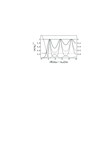
Figure 3: Reciprocal conductivity as a function of harmonic field strength. The right complementary scale is for acceptor impurity sites. The solid curve is $\sigma^{-1}_{sc}$ for $\delta E>0$. The horizontal solid line represents $\sigma^{-1}_{sc}$ for $\delta E<0$, when the impurity sites are empty. The dashed curve shows $\sigma^{-1}_{t}$ up to a factor of $\kappa^{2}$. In this case, only the left scale is appropriate. The dash-dotted curve represents $\sigma^{-1}_{sc}$ for $\delta E>0$ with the singular renormalization factor with $\alpha>0$. For stronger amplifications, the curve follows closer to zero in its minimums. The dotted curve gives a qualitative dependence for finite temperatures at $\delta E\to 0$, $\alpha>0$. In this case, the reciprocal conductivity curve becomes bounded from the bottom (dotted horizontal line)

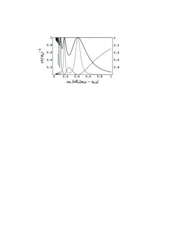
Figure 4: Reciprocal conductivity as a function of harmonic field frequency, $\omega_{0}$. The right complementary scale is for acceptor impurity sites. The curves are cut at low frequency to exclude heavy oscillations. The solid curve is $\sigma^{-1}_{sc}$ for $\delta E>0$. The dashed curve is $\sigma^{-1}_{t}$ up to a factor of $\kappa^{2}$ (only the left scale is appropriate in this case); the dotted curve corresponds to the dash-dotted line in Fig. 3.

Finally, we have two contributions to the conductivity. One is due to the tunneling,

$$\sigma_{t}^{-1}\sim\tau_{t}(E_{F})^{-1}\sim\Delta^{2}J_{0}^{2}(\lambda)\delta^{\prime}(\delta E),$$ (6.3)

where the $\delta$-function $\delta^{\prime}(x)$ is broadened so that $\delta^{\prime}(0)=\kappa^{2}$. The other is caused by scattering,

$$\sigma_{sc}^{-1} \sim \tau_{sc}(E_{F})^{-1}$$

$$\sim \frac{n_{i}\tan^{2}(\delta)\gamma_{in}^{-2}(\lambda)\gamma_{out}^{2}(\lambda)}{\gamma_{in}^{-2}(\lambda)\gamma_{out}^{2}(\lambda)(\cos\delta)^{-2}+\frac{2\gamma_{out}(\lambda)}{\gamma_{in}(\lambda)}+1}.$$

In Figs. 3 and 4, we plot the reciprocal conductivity due to tunneling resonance, Eq. (6.3), and scattering, Eq. (VI), as a function of $\lambda$ and $1/\lambda$. The result is given in terms of the conductivity $\sigma_{0}$ due to the scattering on stationary ionized impurities in the absence of external harmonic field. The tunneling contribution to resistivity, $\sigma_{t}^{-1}$, features the two state aspect of the impurity-2DEG coupling. It reflects the dynamical suppression of resonant tunneling (dynamical localization) similar to the double quantum dot systemsBurdovSolenov1 ; BurdovSolenov2 ; BurdovSolenov3 ; SolenovBurdov where the tunneling is suppressed by $J_{0}(\lambda)$ (or $J_{\bar{m}}(\lambda)$ for lower $E_{0}$ or biased structures) as well. This contribution is proportional to $\Delta^{2}\kappa^{2}$ and vanishes for large fields as $1/\lambda$. It is independent of the donor (acceptor) type of the impurity.

The solid curve in Fig. 3 and 4 show the resistivity due to scattering of conduction electrons on tunneling-active impurities, $\sigma_{sc}^{-1}$. The modification of tunneling is not considered in this case, and the corresponding rates are given by Eqs. (4.5) and (4.6). When $\delta E<0$, the impurity sites are empty at equilibrium and the scattering occurs with the highest probability—the conductivity is not affected by the field. When $\delta E>0$, $\sigma_{sc}^{-1}$ oscillates as a function of $\lambda$. For $\lambda=0$, the occupied impurities do not scatter 2DEG electrons (the situation is opposite for acceptor sites). At $\lambda\gg 1$ tunneling out transitions from higher quasienergies dominate, leaving the impurity empty. The values of resistivity corresponding to $\delta E>0$ and $\delta E<0$ converge to each other, see Fig. 4. In the figure, $\tan\delta=0.1$. For larger values of $V$ the oscillations converge to “1” faster.

When the singular renormalization is introduced, the resistivity peaks become sharper for $\alpha>0$ and $\delta E>0$. The singularity amplifies the tunneling to the impurity site for all $\lambda$ except for near the zeros of $J_{0}(\lambda)$, deactivating the scatterers. The corresponding curves in Figs. 3 and 4 are given for amplification factor of 10. The estimate for small (but finite) temperature with $\delta E\to 0$ is shown as a dotted curve in Fig. 3. In this case, the horizontal line gives the lower bound for large amplifications.

We have investigated tunneling and conductivity modification in impurity-2DEG structure in external time-periodic field. Nonlinear dependence on the field amplitude has been obtained and analyzed for both tunneling rates and conductivity. The calculations have been performed in the limit of small $\Delta$ and nearly zero temperatures. Further investigation has to be done to understand the modification of other 2DEG electron correlations, such as the ones leading to RKKY coupling. The presence of larger currents is also of interest.

Appendix A

We need to analyze the decay of $\langle S(-\infty,t)d(t)d^{\dagger}(t)S(t,-\infty)\rangle$. The scattering matrix is due to the interaction (4.2), with the unperturbed part (4.1). Define the equilibrium Green’s function $G(t,t^{\prime})=-i\langle Td(t)d^{\dagger}(t^{\prime})S(-\infty,\infty)\rangle$. Then, the desired average is $G(t,t^{\prime}\to t\pm 0)$.

Since $\mathbf{H}_{0}$ and $\mathbf{V}$ are time-independent, one can obtain the dynamics by differentiating $G(t,t^{\prime})$ with respect to one of the times. Inverting the operator $i\partial/\partial t^{\prime}-E_{0}$, one obtains

$$G(t-t^{\prime\prime})\!=g(t-t^{\prime\prime})-i\Delta\!\!\ \sum_{m,k}\int\limits_{-\infty}^{\infty}\!\!\!dt^{\prime}M_{m}(t,t^{\prime})g(t^{\prime}-t^{\prime\prime}),$$ (A.1)

where

$$M_{m}(t,t^{\prime})=J_{m}(\lambda)\sum\limits_{n}{(-i)^{n}}\int\limits_{-\infty}^{\infty}{dt_{1}...dt_{n}}$$ (A.2)

$$\times\langle Td(t)V(t_{1})...V(t_{n})c_{k^{\prime}}^{\dagger}(t^{\prime})I_{-}^{(m)}(t^{\prime})\rangle.$$

Here, summation over the connected diagrams is assumed. It is easily noticed that only odd-$n$ terms will contribute to the expression. The first-order term contains the average $\langle Td(t)I_{+}^{(n)}(t_{1})d^{\dagger}(t_{1})c_{k}(t_{1})c_{k^{\prime}}^{\dagger}(t^{\prime})I_{-}^{(m)}(t^{\prime})\rangle$ which splits as $g(t-t_{1})g_{k}(t_{1}-t^{\prime})g_{m}(t_{1}-t^{\prime})$, where $g(t-t_{1})$ and $g_{k}(t_{1}-t^{\prime})$ are noninteracting Green’s functions for impurity and 2DEG electrons, respectively, while $g_{m}(t_{1}-t^{\prime})=e^{im\omega_{0}(t-t^{\prime})}$. The corresponding diagram is

where the solid arrow is $g(t-t_{1})$, the double arrow is $g_{k}(t_{1}-t^{\prime})$, and the dash-arrow represents $g_{m}(t_{1}-t^{\prime})$. The next-order, $n=3$, terms have two $g(t_{1}-t_{2})$ and $g_{k}(t_{1}-t_{2})$ with four spin vertices $I_{\pm}^{(n)}$. Some of the diagrams are

The second (b) diagram represents the fact that averages $\langle I_{+}^{(n_{1})}(t_{1})I_{-}^{(n_{2})}(t_{2})I_{+}^{(n_{3})}(t_{3})I_{-}^{(m)}(t^{\prime})\rangle$ do not necessarily split in pairs—the only restriction is $n_{1}-n_{2}+n_{3}-m=0$. The diagrams of type (a) contribute to a single loop approximate solution,

$$G(\omega)=g(\omega)+g(\omega)\Sigma_{1}(\omega)G(\omega),$$ (A.3)

where the self-energy is

$$\Sigma_{1}(\omega)=\sum\limits_{m,k}{\Delta^{2}}J_{m}^{2}(\lambda)g_{k}(\omega-m\omega_{0}).$$ (A.4)

This result corresponds to the first-order self-energy of the general solution. The other terms can also be evaluated.

Note that operators $I_{\pm}$ describe an asymptotically large spinspincomment and thus commute with each other when averaged over the states corresponding to zero (finite) magnetization, see Eq (III). Therefore, one can replace $I_{\pm}^{(n)}(t)\to e^{\pm in\omega_{0}t}$ with the restriction that the sum of all $\pm n$ in the expression equals zero. After some algebra, the $N$-th order ($N>1$) self-energy can be obtained in the form

$$\Sigma_{N}(\omega) = \!\!\!\!\!\sum\limits_{n_{1},...,n_{2N},k_{1},...,k_{N}}\!\!\!\!{\Delta^{2N}}J_{n_{1}}(\lambda)J_{n_{2}}(-\lambda)...$$

$$\times \delta(n_{1}+n_{2}+...+n_{2N-1}+n_{2N})$$

$$\times g_{k_{1},n_{2},n_{3,4},...}(\omega)g_{n_{3,4},...,n_{2N-1,2N}}(\omega)...$$

$$\times g_{n_{2N-1,2N}}(\omega)g_{k_{N},n_{2N}}(\omega),$$

where the sign of summation indices entering the expression as $-n$ has been changed, $n_{ij}=n_{i}+n_{j}$. We have defined $g_{\xi,\xi^{\prime},...}(\omega)=g(\omega-\omega_{0}\xi-\omega_{0}\xi^{\prime}-...)$ and $g_{k,\xi,\xi^{\prime},...}(\omega)=g_{k}(\omega-\omega_{0}\xi-\omega_{0}\xi^{\prime}-...)$. The summation in Eq. (A) should not include the terms which have $g_{(k),\xi,\xi^{\prime},...}(\omega)$ with $\xi+\xi^{\prime}+...=0$. These terms are taken into account by the preceding self-energies. An estimate of the above sum suggests that $\Sigma_{N}\sim x^{N}$, with $x=\Delta^{2}D_{2}/\omega_{0}$. In our case, $\Delta^{2}D_{2}/\omega_{0}\sim\Delta^{2}/\omega_{0}E_{F}\ll 1$. Therefore, a one-loop approximation is sufficient.

Appendix B

Let us obtain the first-order tunneling rate by averaging the tunneling amplitude subject to evolution due to the Hamiltonian (2.5) without the scattering term. This procedure is similar to the one used in Ref. Keldysh, to study ionization of quantum dot in high-frequency harmonic field. The amplitude for an electron to tunnel from impurity site to the 2DEG states is $\sum\limits_{k}\Delta\langle\bar{d}(t)\bar{c}_{k}^{\dagger}(t)\rangle$. Here, the overbar denotes evolution due to Hamiltonian (2.5) with only the scattering term absent. The first nonvanishing order (with the complex prefactor ignored) is

$$\int\limits_{-\infty}^{\infty}{dt^{\prime}}\sum\limits_{k}{\Delta^{2}}\langle T\tilde{d}(t)\tilde{c}_{k}^{\dagger}(t)\tilde{d}^{\dagger}(t^{\prime})\tilde{c}_{k}(t^{\prime})\rangle,$$ (B.1)

where $\tilde{d}(t)=d\,e^{-iE_{0}t-i\frac{{V_{00}}}{{\omega_{0}}}\sin\omega_{0}t}$ and $\tilde{c}_{k}(t)=c_{k}e^{-iE_{k}t-i\frac{{V_{2DEG}}}{{\omega_{0}}}\sin\omega_{0}t}$. These expressions are substituted into Eq. (B.1) to obtain

$$\int\limits_{-\infty}^{\infty}{dt^{\prime}}\sum\limits_{k}{\Delta^{2}}\langle Td(t)c_{k}^{\dagger}(t)d^{\dagger}(t^{\prime})c_{k}(t^{\prime})\rangle$$ (B.2)

$$\times\sum\limits_{nn^{\prime}}{J_{n}(\lambda)J_{n^{\prime}}(\lambda)}e^{-in\omega_{0}t}e^{in^{\prime}\omega_{0}t^{\prime}},$$ (B.3)

expanding the oscillatory exponents into the Bessel series. Here, $d(t)=d\,e^{-iE_{0}t}$ and $c_{k}(t)=c_{k}e^{-iE_{k}t}$. The amplitude is then averaged over the fast driving field oscillations yielding

$$\sum\limits_{n}{J_{n}^{2}(\lambda)}\!\!\!\int\limits_{-\infty}^{\infty}\!\!{dt^{\prime}}\sum\limits_{k}{\Delta^{2}}\langle Td(t)c_{k}^{\dagger}(t)d^{\dagger}(t^{\prime})c_{k}(t^{\prime})\rangle e^{in\omega_{0}\left({t^{\prime}-t}\right)}.$$ (B.4)

After the integration, one finally obtains the rates proportional to

$$\mathrm{Im}\sum\limits_{n}{\Delta^{2}J_{n}^{2}(\lambda)}\sum\limits_{k}{\frac{\theta(\pm 1)\mp n_{k}}{{E_{0}-E_{k}-\omega_{0}n\pm i0}}},$$ (B.5)

which gives Eq. (4.3) with $\omega\to E_{0}$.

References

- (1) M. Xiao, I. Martin, E. Yablonovitch, and H. W. Jiang, Nature 430, 435 (2004).
- (2) M. R. Sakr, H. W. Jiang, E. Yablonovitch, and E. T. Croke, Appl. Phys. Lett. 87, 223104 (2005).
- (3) N. J. Craig, J. M. Taylor, E. A. Lester, C. M. Marcus, M. P. Hanson, and A. C. Gossard, Science 304, 565 (2004).
- (4) J. M. Elzerman, R. Hanson, L. H. Willems van Beveren, B. Witkamp, L. M. K. Vandersypen, and L. P. Kouwenhoven, Nature 430, 431 (2004).
- (5) F. H. L. Koppens, C. Buizert, K. J. Tielrooij, I. T. Vink, K. C. Nowack, T. Meunier, L. P. Kouwenhoven, and L. M. K. Vandersypen, Nature 442, 766 (2006).
- (6) D. H. Dunlap and V. M. Kenkre, Phys. Rev. B 34, 3625 (1986).
- (7) F. Grossmann, T. Dittrich, P. Jung and P. Hanggi, Phys. Rev. Lett. 67, 516 (1991).
- (8) F. Grossmann and P. Hanggi, Europhys. Lett. 18, 571 (1992).
- (9) Y. Dakhnovskii and R. Bavli, Phys. Rev. B 48, 11010 (1993).
- (10) R. Bavli and H. Metiu, Phys. Rev. A 47, 3299 (1993).
- (11) M. Holthaus and D. Hone, Phys. Rev. B 47, 6499 (1993).
- (12) S. Raghavan, V. M. Kenkre, D. H. Dunlap, A. R. Bishop, and M. I. Salkola, Phys. Rev. A 54, R1781 (1996).
- (13) M. Grifoni and P. Hanggi, Phys. Rep. 304, 229 (1998).
- (14) V. A. Burdov, Zh. Eksp. Teor. Fiz. 116, 217 (1999) [JETP 89, 119 (1999)].
- (15) V. A. Burdov, Pis’ma Zh. Eksp. Teor. Fiz. 76, 25 (2002) [JETP Lett. 76, 21 (2002)].
- (16) V. A. Burdov and D. S. Solenov, Phys. Lett. A 305, 427 (2002).
- (17) V. A. Burdov and D. S. Solenov, Phys. E 24, 217 (2004).
- (18) V. A. Burdov and D. S. Solenov, Zh. Eksp. Teor. Fiz. 125, 684 (2004) [JETP 98, 605 (2004)].
- (19) Y. A. Romanov and J. Y. Romanova, Zh. Eksp. Teor. Fiz. 118, 1193 (2000); J. Y. Romanova and Y. A. Romanov, e-print: cond-mat/0612550 at www.arXiv.org.
- (20) R. M. Lewis, Y. P. Chen, L. W. Engel, D. C. Tsui, L. N. Pfeiffer, and K. W. West, Phys. Rev. B 71, 081301 (2005).
- (21) K. S. Ralls, W. J. Skocpol, L. D. Jackel, R. E. Howard, L. A. Fetter, R. W. Epworth, and D. M. Tennant, Phys. Rev. Lett. 52, 228 (1984).
- (22) D. Mozyrsky, I. Martin, A. Shnirman, and M. B. Hastings, e-print: cond-mat/0312503 at www.arXiv.org.
- (23) P. D. Ye, L. W. Engel, D. C. Tsui, J. A. Simmons, J. R. Wendt, G. A. Vawter, and J. L. Reno, Appl. Phys. Lett. 79, 2193 (2001).
- (24) J. H. Shirley, Phys. Rev. B 138, 979 (1965).
- (25) Ya. B. Zel’dovich, Zh. Eksp. Teor. Fiz. 51, 1492 (1966) [Sov. Phys. JETP 24, 1006 (1967)].
- (26) V. I. Ritus, Zh. Eksp. Teor. Fiz. 51, 1544 (1966) [Sov. Phys. JETP 24, 1041 (1967)].
- (27) D. Solenov and V. A. Burdov, Phys. Rev. B 72, 085347 (2005).
- (28) The actual spin operators do not yield a properly normalized state. In particular, , , . In our case, we are interested in the limit while keeping finite. In terms of Eq. (3.5), this means that only the terms with finite frequency are of interest when calculating the averages. Therefore , , and one can use in the Hamiltonian (3.7).
- (29) In addition to the fact that the tunneling amplitude is relatively small even for close impurities, it is often renormalized (suppressed) by the phonon dressing, see, for example, Ref. Mozyrsky, .
- (30) P. Nozieres and C. T. De Dominics, Phys. Rev. 178, 1097 (1969).
- (31) The time scale of equilibration on the single impurity site, , should be smaller than the time between collisions on different impurities.
- (32) G. D. Mahan, Many-Particle Physics (Kluwer Academic, New York, 2000).
- (33) The additional angular dependence in the Boltzmann result for the conductivity accounts for the change of the momenta direction, , as the result of the collision event. In our case, the external field affects only the overall strength of the scattering event. Therefore, one expects the field dependence to be the same for both relaxation times.
- (34) When proper angular dependence is considered, the right-hand side of this expression acquires the summation over the angular function distribution.NozieresDominics ; Mahan The dependence, however, should not be altered.
- (35) L. V. Keldysh, Zh. Eksp. Teor. Fiz. 47, 1945 (1964).