Study of K 0 → π − e + ν e e + e − → superscript 𝐾 0 superscript 𝜋 superscript 𝑒 subscript 𝜈 𝑒 superscript 𝑒 superscript 𝑒 K^{0}\rightarrow\pi^{-}e^{+}\nu_{e}e^{+}e^{-}
K. Tsuji and T. Sato
Department of Physics, Osaka University, Toyonaka, Osaka 560-0043, Japan
Abstract
K 0 → π − e + ν e e + e − → superscript 𝐾 0 superscript 𝜋 superscript 𝑒 subscript 𝜈 𝑒 superscript 𝑒 superscript 𝑒 K^{0}\rightarrow\pi^{-}e^{+}\nu_{e}e^{+}e^{-} 𝒪 ( 4 ) superscript 𝒪 4 {\mathcal{O}}^{(4)} 𝒪 ( 4 ) superscript 𝒪 4 {\mathcal{O}}^{(4)} 3 e ν 3 𝑒 𝜈 3e\nu
pacs: 13.20.Eb, 12.39.Fe, 11.30.Rd, 12.40.Yx
I introduction
The radiative semileptonic kaon decay,
K L → π ± e ∓ ν γ → subscript 𝐾 𝐿 superscript 𝜋 plus-or-minus superscript 𝑒 minus-or-plus 𝜈 𝛾 K_{L}\rightarrow\pi^{\pm}e^{\mp}\nu\gamma K l 3 γ subscript 𝐾 𝑙 3 𝛾 K_{l3\gamma} ktev-2 ; ktev-3 ; na48-2 ; fearing-1 ; holstein ; bijnens-2 ; gasser-2 ; kubis ; moulson ; bijnens gasser-1 K l 3 γ subscript 𝐾 𝑙 3 𝛾 K_{l3\gamma} 𝒪 ( q − 1 ) 𝒪 superscript 𝑞 1 {\mathcal{O}}(q^{-1}) 𝒪 ( q 0 ) 𝒪 superscript 𝑞 0 {\mathcal{O}}(q^{0}) q 𝑞 q K l 3 subscript 𝐾 𝑙 3 K_{l3} low adler 𝒪 ( q ) 𝒪 𝑞 {\mathcal{O}}(q) K L → π ± e ∓ ν γ ( K l 3 γ ) → subscript 𝐾 𝐿 superscript 𝜋 plus-or-minus superscript 𝑒 minus-or-plus 𝜈 𝛾 subscript 𝐾 𝑙 3 𝛾 K_{L}\rightarrow\pi^{\pm}e^{\mp}\nu\gamma(K_{l3\gamma})
Fearing et al.fearing-1 studied the radiative K l 3 subscript 𝐾 𝑙 3 K_{l3} holstein 𝒪 ( p 4 ) 𝒪 superscript 𝑝 4 {\mathcal{O}}(p^{4}) 𝒪 ( p 4 ) 𝒪 superscript 𝑝 4 {\mathcal{O}}(p^{4}) et al. bijnens-2 K e 3 γ subscript 𝐾 𝑒 3 𝛾 K_{e3\gamma} 𝒪 ( p 6 ) 𝒪 superscript 𝑝 6 {\mathcal{O}}(p^{6}) et al. gasser-2 ; kubis moulson bijnens
In this paper, we report on
a ChPT study of the semileptonic decay process of kaon
K 0 → π − e + ν e e + e − → superscript 𝐾 0 superscript 𝜋 superscript 𝑒 subscript 𝜈 𝑒 superscript 𝑒 superscript 𝑒 K^{0}\rightarrow\pi^{-}e^{+}\nu_{e}e^{+}e^{-} K e 3 e + e − 0 subscript superscript 𝐾 0 𝑒 3 superscript 𝑒 superscript 𝑒 K^{0}_{e3e^{+}e^{-}} K L → π ± e ∓ ν γ → subscript 𝐾 𝐿 superscript 𝜋 plus-or-minus superscript 𝑒 minus-or-plus 𝜈 𝛾 K_{L}\rightarrow\pi^{\pm}e^{\mp}\nu\gamma K l 3 γ subscript 𝐾 𝑙 3 𝛾 K_{l3\gamma} e + e − superscript 𝑒 superscript 𝑒 e^{+}e^{-} kotera e + e − superscript 𝑒 superscript 𝑒 e^{+}e^{-} M e + e − subscript 𝑀 superscript 𝑒 superscript 𝑒 M_{e^{+}e^{-}} M 3 e ν subscript 𝑀 3 𝑒 𝜈 M_{3e\nu} 𝒪 ( p 4 ) 𝒪 superscript 𝑝 4 {\mathcal{O}}(p^{4}) K e 3 e + e − 0 subscript superscript 𝐾 0 𝑒 3 superscript 𝑒 superscript 𝑒 K^{0}_{e3e^{+}e^{-}} 𝒪 ( p 4 ) 𝒪 superscript 𝑝 4 {\mathcal{O}}(p^{4}) K l 3 e + e − 0 ( l = e , μ ) subscript superscript 𝐾 0 𝑙 3 superscript 𝑒 superscript 𝑒 𝑙 𝑒 𝜇
K^{0}_{l3e^{+}e^{-}}(l=e,\mu) K l 3 0 subscript superscript 𝐾 0 𝑙 3 K^{0}_{l3}
In section II, we summarize the effective Lagrangian employed in
this work. The explicit form of the amplitudes of
K l 3 e + e − 0 ( l = e , μ ) subscript superscript 𝐾 0 𝑙 3 superscript 𝑒 superscript 𝑒 𝑙 𝑒 𝜇
K^{0}_{l3e^{+}e^{-}}(l=e,\mu) 𝒪 ( p 4 ) 𝒪 superscript 𝑝 4 {\mathcal{O}}(p^{4}) K l 3 e + e − 0 ( l = e , μ ) subscript superscript 𝐾 0 𝑙 3 superscript 𝑒 superscript 𝑒 𝑙 𝑒 𝜇
K^{0}_{l3e^{+}e^{-}}(l=e,\mu) 𝒪 ( p 4 ) 𝒪 superscript 𝑝 4 {\mathcal{O}}(p^{4})
II Effective Lagrangian
Chiral perturbation theory is an effective field theory of QCD
to describe low energy hadronic system using a systematic
perturbation scheme. In this section, a standard effective
Lagrangian of ChPT for Goldstone bosons gasser-1 ; scherer U ( x ) 𝑈 𝑥 U(x) ϕ a subscript italic-ϕ 𝑎 \phi_{a}
U = exp ( i ϕ ( x ) F 0 ) , 𝑈 𝑖 italic-ϕ 𝑥 subscript 𝐹 0 U=\exp\left(i\frac{\phi(x)}{F_{0}}\right),\qquad (1)
with
ϕ ( x ) = ∑ a = 1 8 λ a ϕ a ( x ) . italic-ϕ 𝑥 superscript subscript 𝑎 1 8 subscript 𝜆 𝑎 subscript italic-ϕ 𝑎 𝑥 \phi(x)=\sum_{a=1}^{8}\lambda_{a}\phi_{a}(x). (2)
Here F 0 subscript 𝐹 0 F_{0} λ a subscript 𝜆 𝑎 \lambda_{a} gasser-1 ; scherer 𝒪 ( p 2 ) 𝒪 superscript 𝑝 2 {\mathcal{O}}(p^{2})
ℒ ( 2 ) = F 0 2 4 < D μ U ( D μ U ) † + χ U † + U χ † > . superscript ℒ 2 superscript subscript 𝐹 0 2 4 expectation subscript 𝐷 𝜇 𝑈 superscript superscript 𝐷 𝜇 𝑈 † 𝜒 superscript 𝑈 † 𝑈 superscript 𝜒 † {\mathcal{L}}^{(2)}=\frac{F_{0}^{2}}{4}<D_{\mu}U(D^{\mu}U)^{\dagger}+\chi U^{\dagger}+U\chi^{\dagger}>. (3)
< O > expectation 𝑂 <O> O 𝑂 O χ 𝜒 \chi χ = 2 B 0 M 𝜒 2 subscript 𝐵 0 𝑀 \chi=2B_{0}M M = diag ( m u , m d , m s ) 𝑀 diag subscript 𝑚 𝑢 subscript 𝑚 𝑑 subscript 𝑚 𝑠 M=\textrm{diag}(m_{u},m_{d},m_{s}) B 0 subscript 𝐵 0 B_{0} D μ U subscript 𝐷 𝜇 𝑈 D_{\mu}U A μ subscript 𝐴 𝜇 A_{\mu} W μ subscript 𝑊 𝜇 W_{\mu}
D μ U subscript 𝐷 𝜇 𝑈 \displaystyle D_{\mu}U = \displaystyle= ∂ μ U − i r μ U + i U l μ , subscript 𝜇 𝑈 𝑖 subscript 𝑟 𝜇 𝑈 𝑖 𝑈 subscript 𝑙 𝜇 \displaystyle\partial_{\mu}U-ir_{\mu}U+iUl_{\mu}, (4)
r μ subscript 𝑟 𝜇 \displaystyle r_{\mu} = \displaystyle= v μ + a μ = − e Q A μ , subscript 𝑣 𝜇 subscript 𝑎 𝜇 𝑒 𝑄 subscript 𝐴 𝜇 \displaystyle v_{\mu}+a_{\mu}=-eQA_{\mu}, (5)
l μ subscript 𝑙 𝜇 \displaystyle l_{\mu} = \displaystyle= v μ − a μ = − e Q A μ − g 2 ( W μ + T + + h.c. ) . subscript 𝑣 𝜇 subscript 𝑎 𝜇 𝑒 𝑄 subscript 𝐴 𝜇 𝑔 2 superscript subscript 𝑊 𝜇 subscript 𝑇 h.c. \displaystyle v_{\mu}-a_{\mu}=-eQA_{\mu}-\frac{g}{\sqrt{2}}(W_{\mu}^{+}T_{+}+\textrm{h.c.}). (6)
Q 𝑄 Q T + subscript 𝑇 T_{+}
Q = 1 3 ( 2 0 0 0 − 1 0 0 0 − 1 ) , T + = ( 0 V u d V u s 0 0 0 0 0 0 ) . formulae-sequence 𝑄 1 3 2 0 0 0 1 0 0 0 1 subscript 𝑇 0 subscript 𝑉 𝑢 𝑑 subscript 𝑉 𝑢 𝑠 0 0 0 0 0 0 Q=\frac{1}{3}\left(\begin{array}[]{ccc}2&0&0\\
0&-1&0\\
0&0&-1\end{array}\right),\qquad T_{+}=\left(\begin{array}[]{ccc}0&V_{ud}&V_{us}\\
0&0&0\\
0&0&0\end{array}\right). (7)
The next to-leading-order (NLO) 𝒪 ( p 4 ) 𝒪 superscript 𝑝 4 {\mathcal{O}}(p^{4}) gasser-1
ℒ ( 4 ) superscript ℒ 4 \displaystyle\mathcal{L}^{(4)} = \displaystyle= L 1 < D μ U ( D μ U ) † > 2 + L 2 < D μ U ( D ν U ) † > < D μ U ( D ν U ) † > subscript 𝐿 1 superscript expectation subscript 𝐷 𝜇 𝑈 superscript superscript 𝐷 𝜇 𝑈 † 2 subscript 𝐿 2 expectation subscript 𝐷 𝜇 𝑈 superscript subscript 𝐷 𝜈 𝑈 † expectation superscript 𝐷 𝜇 𝑈 superscript superscript 𝐷 𝜈 𝑈 † \displaystyle L_{1}<D_{\mu}U(D^{\mu}U)^{\dagger}>^{2}+L_{2}<D_{\mu}U(D_{\nu}U)^{\dagger}><D^{\mu}U(D^{\nu}U)^{\dagger}> (8)
+ L 3 < D μ U ( D μ U ) † D ν U ( D ν U ) † > + L 4 < D μ U ( D μ U ) † > < χ U † + U χ † > subscript 𝐿 3 expectation subscript 𝐷 𝜇 𝑈 superscript superscript 𝐷 𝜇 𝑈 † subscript 𝐷 𝜈 𝑈 superscript superscript 𝐷 𝜈 𝑈 † subscript 𝐿 4 expectation subscript 𝐷 𝜇 𝑈 superscript superscript 𝐷 𝜇 𝑈 † expectation 𝜒 superscript 𝑈 † 𝑈 superscript 𝜒 † \displaystyle+L_{3}<D_{\mu}U(D^{\mu}U)^{\dagger}D_{\nu}U(D^{\nu}U)^{\dagger}>+L_{4}<D_{\mu}U(D^{\mu}U)^{\dagger}><\chi U^{\dagger}+U\chi^{\dagger}>
+ L 5 < D μ U ( D μ U ) † ( χ U † + U χ † ) > + L 6 < χ U † + U χ † > 2 subscript 𝐿 5 expectation subscript 𝐷 𝜇 𝑈 superscript superscript 𝐷 𝜇 𝑈 † 𝜒 superscript 𝑈 † 𝑈 superscript 𝜒 † subscript 𝐿 6 superscript expectation 𝜒 superscript 𝑈 † 𝑈 superscript 𝜒 † 2 \displaystyle+L_{5}<D_{\mu}U(D^{\mu}U)^{\dagger}(\chi U^{\dagger}+U\chi^{\dagger})>+L_{6}<\chi U^{\dagger}+U\chi^{\dagger}>^{2}
+ L 7 < χ † U − U † χ > 2 + L 8 < χ U † χ U † + U χ † U χ † > subscript 𝐿 7 superscript expectation superscript 𝜒 † 𝑈 superscript 𝑈 † 𝜒 2 subscript 𝐿 8 expectation 𝜒 superscript 𝑈 † 𝜒 superscript 𝑈 † 𝑈 superscript 𝜒 † 𝑈 superscript 𝜒 † \displaystyle+L_{7}<\chi^{\dagger}U-U^{\dagger}\chi>^{2}+L_{8}<\chi U^{\dagger}\chi U^{\dagger}+U\chi^{\dagger}U\chi^{\dagger}>
− i L 9 < f μ ν R D μ U ( D ν U ) † + f μ ν L D μ D ( D ν U ) † > + L 10 < U f μ ν L U † f R μ ν > , 𝑖 subscript 𝐿 9 expectation superscript subscript 𝑓 𝜇 𝜈 𝑅 superscript 𝐷 𝜇 𝑈 superscript superscript 𝐷 𝜈 𝑈 † superscript subscript 𝑓 𝜇 𝜈 𝐿 superscript 𝐷 𝜇 𝐷 superscript superscript 𝐷 𝜈 𝑈 † subscript 𝐿 10 expectation 𝑈 subscript superscript 𝑓 𝐿 𝜇 𝜈 superscript 𝑈 † superscript subscript 𝑓 𝑅 𝜇 𝜈 \displaystyle-iL_{9}<f_{\mu\nu}^{R}D^{\mu}U(D^{\nu}U)^{\dagger}+f_{\mu\nu}^{L}D^{\mu}D(D^{\nu}U)^{\dagger}>+L_{10}<Uf^{L}_{\mu\nu}U^{\dagger}f_{R}^{\mu\nu}>,
with
f μ ν R ( L ) subscript superscript 𝑓 𝑅 𝐿 𝜇 𝜈 \displaystyle f^{R(L)}_{\mu\nu} = \displaystyle= ∂ μ r ( l ) ν − ∂ ν r ( l ) μ − i [ r ( l ) μ , r ( l ) ν ] , subscript 𝜇 𝑟 subscript 𝑙 𝜈 subscript 𝜈 𝑟 subscript 𝑙 𝜇 𝑖 𝑟 subscript 𝑙 𝜇 𝑟 subscript 𝑙 𝜈 \displaystyle\partial_{\mu}r(l)_{\nu}-\partial_{\nu}r(l)_{\mu}-i[r(l)_{\mu},r(l)_{\nu}], (9)
and its filed tensors are defined as
f μ ν R subscript superscript 𝑓 𝑅 𝜇 𝜈 \displaystyle f^{R}_{\mu\nu} = \displaystyle= ∂ μ r ν − ∂ ν r μ − i [ r μ , r ν ] , subscript 𝜇 subscript 𝑟 𝜈 subscript 𝜈 subscript 𝑟 𝜇 𝑖 subscript 𝑟 𝜇 subscript 𝑟 𝜈 \displaystyle\partial_{\mu}r_{\nu}-\partial_{\nu}r_{\mu}-i[r_{\mu},r_{\nu}], (10)
f μ ν L subscript superscript 𝑓 𝐿 𝜇 𝜈 \displaystyle f^{L}_{\mu\nu} = \displaystyle= ∂ μ l ν − ∂ ν l μ − i [ l μ , l ν ] . subscript 𝜇 subscript 𝑙 𝜈 subscript 𝜈 subscript 𝑙 𝜇 𝑖 subscript 𝑙 𝜇 subscript 𝑙 𝜈 \displaystyle\partial_{\mu}l_{\nu}-\partial_{\nu}l_{\mu}-i[l_{\mu},l_{\nu}]. (11)
The following piece of the chiral anomaly term wz ; witten 𝒪 ( p 4 ) 𝒪 superscript 𝑝 4 {\mathcal{O}}(p^{4}) K e 3 e + e − 0 subscript superscript 𝐾 0 𝑒 3 superscript 𝑒 superscript 𝑒 K^{0}_{e3e^{+}e^{-}}
ℒ a n o m ( 4 ) subscript superscript ℒ 4 𝑎 𝑛 𝑜 𝑚 \displaystyle{\mathcal{L}}^{(4)}_{anom} = \displaystyle= − i e g 16 2 π 2 ϵ μ ν ρ σ W μ + ∂ ν A ρ < T + { ∂ σ U † Q U − 2 U † ∂ σ U Q − 2 Q U † ∂ σ U − U † Q ∂ σ U } > 𝑖 𝑒 𝑔 16 2 superscript 𝜋 2 superscript italic-ϵ 𝜇 𝜈 𝜌 𝜎 subscript superscript 𝑊 𝜇 subscript 𝜈 subscript 𝐴 𝜌 expectation subscript 𝑇 subscript 𝜎 superscript 𝑈 † 𝑄 𝑈 2 superscript 𝑈 † subscript 𝜎 𝑈 𝑄 2 𝑄 superscript 𝑈 † subscript 𝜎 𝑈 superscript 𝑈 † 𝑄 subscript 𝜎 𝑈 \displaystyle-\frac{ieg}{16\sqrt{2}\pi^{2}}\epsilon^{\mu\nu\rho\sigma}W^{+}_{\mu}\partial_{\nu}A_{\rho}\bigg{<}T_{+}\left\{\partial_{\sigma}U^{\dagger}QU-2U^{\dagger}\partial_{\sigma}UQ-2QU^{\dagger}\partial_{\sigma}U-U^{\dagger}Q\partial_{\sigma}U\right\}\bigg{>} (12)
+ h.c. . h.c. \displaystyle+\textrm{h.c.}.
III LO and NLO amplitudes of K e 3 e + e − 0 subscript superscript 𝐾 0 𝑒 3 superscript 𝑒 superscript 𝑒 K^{0}_{e3e^{+}e^{-}}
Using the chiral effective Lagrangian presented in the previous section,
we study the amplitude of K e 3 e + e − 0 subscript superscript 𝐾 0 𝑒 3 superscript 𝑒 superscript 𝑒 K^{0}_{e3e^{+}e^{-}}
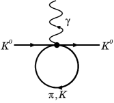
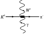
K 0 ( p 1 ) → π − ( p 2 ) + e + ( k 1 ) + ν e ( k 2 ) + e + ( k 3 ) + e − ( k 4 ) . → superscript 𝐾 0 subscript 𝑝 1 superscript 𝜋 subscript 𝑝 2 superscript 𝑒 subscript 𝑘 1 subscript 𝜈 𝑒 subscript 𝑘 2 superscript 𝑒 subscript 𝑘 3 superscript 𝑒 subscript 𝑘 4 K^{0}(p_{1})\rightarrow\pi^{-}(p_{2})+\,e^{+}(k_{1})\,+\nu_{e}(k_{2})\,+e^{+}(k_{3})\,+e^{-}(k_{4}). (13)
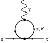
The momentum of the virtual photon q μ superscript 𝑞 𝜇 q^{\mu} q μ = k 3 μ + k 4 μ superscript 𝑞 𝜇 superscript subscript 𝑘 3 𝜇 superscript subscript 𝑘 4 𝜇 q^{\mu}=k_{3}^{\mu}+k_{4}^{\mu} T ( 2 ) superscript 𝑇 2 T^{(2)} ℒ ( 2 ) superscript ℒ 2 {\mathcal{L}}^{(2)} ℒ ( 2 ) superscript ℒ 2 {\mathcal{L}}^{(2)} ℒ ( 4 ) superscript ℒ 4 {\mathcal{L}}^{(4)} T ( 4 ) superscript 𝑇 4 T^{(4)}
Figure 1: The leading order diagrams
contributing to the K e 3 e + e − 0 subscript superscript 𝐾 0 𝑒 3 superscript 𝑒 superscript 𝑒 K^{0}_{e3e^{+}e^{-}} ℒ ( 2 ) superscript ℒ 2 {\mathcal{L}}^{(2)}
The leading order amplitude T ( 2 ) superscript 𝑇 2 T^{(2)} K e 3 e + e − 0 subscript superscript 𝐾 0 𝑒 3 superscript 𝑒 superscript 𝑒 K^{0}_{e3e^{+}e^{-}} 1
T ( 2 ) superscript 𝑇 2 \displaystyle T^{(2)} = \displaystyle= − G F 2 e 2 V u s ∗ 1 q 2 [ u ¯ ( k 2 ) { g μ ν − 2 q ν p 2 μ ( p 2 + q ) 2 − m π 2 } γ ν ( 1 − γ 5 ) v ( k 1 ) \displaystyle-\frac{G_{F}}{\sqrt{2}}e^{2}V_{us}^{*}\frac{1}{q^{2}}\bigg{[}\bar{u}(k_{2})\left\{g_{\mu\nu}-\frac{2q_{\nu}p_{2\mu}}{(p_{2}+q)^{2}-m_{\pi}^{2}}\right\}\gamma^{\nu}(1-\gamma_{5})v(k_{1})
+ u ¯ ( k 2 ) ( p 1 + p 2 ) ( 1 − γ 5 ) { 2 k 1 μ + q γ μ ( k 1 + q ) 2 − m e 2 − 2 p 2 μ ( p 2 + q ) 2 − m π 2 } v ( k 1 ) ] u ¯ ( k 4 ) γ μ v ( k 3 ) . \displaystyle+\bar{u}(k_{2})(\not\!p_{1}+\not\!p_{2})(1-\gamma_{5})\left\{\frac{2k_{1\mu}+\not\!q\gamma_{\mu}}{(k_{1}+q)^{2}-m_{e}^{2}}-\frac{2p_{2\mu}}{(p_{2}+q)^{2}-m_{\pi}^{2}}\right\}v(k_{1})\bigg{]}\bar{u}(k_{4})\gamma^{\mu}v(k_{3}).
Here G F subscript 𝐺 𝐹 G_{F} V u s subscript 𝑉 𝑢 𝑠 V_{us} LABEL:leading )
represents the ’direct amplitude’. The ’exchange amplitude’ is given
from Eq. (LABEL:leading ) by interchanging momentum and spins of the
two positrons and by taking into account the phase ( − 1 ) 1 (-1) LABEL:leading ) satisfies gauge invariance and agrees with Eq.
(5.12) of Ref. bijnens-2 e + e − superscript 𝑒 superscript 𝑒 e^{+}e^{-}
e q 2 u ¯ ( k 4 ) γ μ v ( k 3 ) = ϵ ∗ μ . 𝑒 superscript 𝑞 2 ¯ 𝑢 subscript 𝑘 4 superscript 𝛾 𝜇 𝑣 subscript 𝑘 3 superscript italic-ϵ absent 𝜇 \frac{e}{q^{2}}\bar{u}(k_{4})\gamma^{\mu}v(k_{3})=\epsilon^{*\mu}. (15)
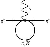
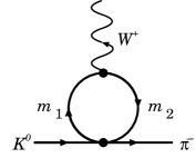
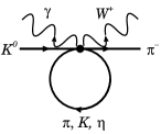
At the NLO, loop corrections and contributions of ℒ ( 4 ) superscript ℒ 4 \mathcal{L}^{(4)} 2 2 2 π K W 𝜋 𝐾 𝑊 \pi KW 2 2 K π W γ 𝐾 𝜋 𝑊 𝛾 K\pi W\gamma 2 2 T ( 4 ) superscript 𝑇 4 T^{(4)}
T ( 4 ) = T ( a ) ( 4 ) + T ( b ) ( 4 ) + T ( c ) ( 4 ) + T ( d ) ( 4 ) + T ( e ) ( 4 ) + T ( e , a n o m ) ( 4 ) . superscript 𝑇 4 subscript superscript 𝑇 4 𝑎 subscript superscript 𝑇 4 𝑏 subscript superscript 𝑇 4 𝑐 subscript superscript 𝑇 4 𝑑 subscript superscript 𝑇 4 𝑒 subscript superscript 𝑇 4 𝑒 𝑎 𝑛 𝑜 𝑚 T^{(4)}=T^{(4)}_{(a)}+T^{(4)}_{(b)}+T^{(4)}_{(c)}+T^{(4)}_{(d)}+T^{(4)}_{(e)}+T^{(4)}_{(e,anom)}. (16)
For completeness, the explicit forms of T ( i ) ( 4 ) subscript superscript 𝑇 4 𝑖 T^{(4)}_{(i)} T ( 4 ) superscript 𝑇 4 T^{(4)} bijnens-2
Figure 2: The NLO diagrams contributing to the K e 3 e + e − 0 subscript superscript 𝐾 0 𝑒 3 superscript 𝑒 superscript 𝑒 K^{0}_{e3e^{+}e^{-}}
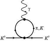
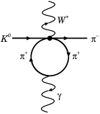
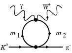
III.1 Pion and neutral kaon form factor
In K e 3 e + e − 0 subscript superscript 𝐾 0 𝑒 3 superscript 𝑒 superscript 𝑒 K^{0}_{e3e^{+}e^{-}} 3 3 3 3 ℒ ( 4 ) superscript ℒ 4 {\mathcal{L}}^{(4)} 3 T ( a ) ( 4 ) subscript superscript 𝑇 4 𝑎 T^{(4)}_{(a)} T ( b ) ( 4 ) subscript superscript 𝑇 4 𝑏 T^{(4)}_{(b)}
T ( a ) ( 4 ) subscript superscript 𝑇 4 𝑎 \displaystyle T^{(4)}_{(a)} = \displaystyle= − G F 2 e 2 V u s ∗ H π ( q 2 ) q 2 [ u ¯ ( k 2 ) ( p 1 + p 2 + q ) ( 1 − γ 5 ) − 2 p 2 μ ( p 2 + q ) 2 − m π 2 v ( k 1 ) ] u ¯ ( k 4 ) γ μ v ( k 3 ) , subscript 𝐺 𝐹 2 superscript 𝑒 2 superscript subscript 𝑉 𝑢 𝑠 superscript 𝐻 𝜋 superscript 𝑞 2 superscript 𝑞 2 delimited-[] ¯ 𝑢 subscript 𝑘 2 subscript 𝑝 1 subscript 𝑝 2 𝑞 1 subscript 𝛾 5 2 subscript 𝑝 2 𝜇 superscript subscript 𝑝 2 𝑞 2 superscript subscript 𝑚 𝜋 2 𝑣 subscript 𝑘 1 ¯ 𝑢 subscript 𝑘 4 superscript 𝛾 𝜇 𝑣 subscript 𝑘 3 \displaystyle-\frac{G_{F}}{\sqrt{2}}e^{2}V_{us}^{*}\frac{H^{\pi}(q^{2})}{q^{2}}\left[\bar{u}(k_{2})(\not\!p_{1}+\not\!p_{2}+\not\!q)(1-\gamma_{5})\frac{-2p_{2\mu}}{(p_{2}+q)^{2}-m_{\pi}^{2}}v(k_{1})\right]\bar{u}(k_{4})\gamma^{\mu}v(k_{3}),
T ( b ) ( 4 ) subscript superscript 𝑇 4 𝑏 \displaystyle T^{(4)}_{(b)} = \displaystyle= − G F 2 e 2 V u s ∗ H K ( q 2 ) q 2 [ u ¯ ( k 2 ) ( p 1 + p 2 − q ) ( 1 − γ 5 ) 2 p 1 μ ( p 1 − q ) 2 − m K 2 v ( k 1 ) ] u ¯ ( k 4 ) γ μ v ( k 3 ) . subscript 𝐺 𝐹 2 superscript 𝑒 2 superscript subscript 𝑉 𝑢 𝑠 superscript 𝐻 𝐾 superscript 𝑞 2 superscript 𝑞 2 delimited-[] ¯ 𝑢 subscript 𝑘 2 subscript 𝑝 1 subscript 𝑝 2 𝑞 1 subscript 𝛾 5 2 subscript 𝑝 1 𝜇 superscript subscript 𝑝 1 𝑞 2 superscript subscript 𝑚 𝐾 2 𝑣 subscript 𝑘 1 ¯ 𝑢 subscript 𝑘 4 superscript 𝛾 𝜇 𝑣 subscript 𝑘 3 \displaystyle-\frac{G_{F}}{\sqrt{2}}e^{2}V_{us}^{*}\frac{H^{K}(q^{2})}{q^{2}}\left[\bar{u}(k_{2})(\not\!p_{1}+\not\!p_{2}-\not\!q)(1-\gamma_{5})\frac{2p_{1\mu}}{(p_{1}-q)^{2}-m_{K}^{2}}v(k_{1})\right]\bar{u}(k_{4})\gamma^{\mu}v(k_{3}).
Here we define q = p 1 − p 2 𝑞 subscript 𝑝 1 subscript 𝑝 2 q=p_{1}-p_{2} H π superscript 𝐻 𝜋 H^{\pi} H K superscript 𝐻 𝐾 H^{K}
H π ( q 2 ) superscript 𝐻 𝜋 superscript 𝑞 2 \displaystyle H^{\pi}(q^{2}) = \displaystyle= 1 F 0 2 [ 2 L 9 q 2 + A ( m π 2 ) + 1 2 A ( m K 2 ) − 2 B 22 ( m π 2 , m π 2 , q 2 ) − B 22 ( m K 2 , m K 2 , q 2 ) ] , 1 superscript subscript 𝐹 0 2 delimited-[] 2 subscript 𝐿 9 superscript 𝑞 2 𝐴 superscript subscript 𝑚 𝜋 2 1 2 𝐴 superscript subscript 𝑚 𝐾 2 2 subscript 𝐵 22 superscript subscript 𝑚 𝜋 2 superscript subscript 𝑚 𝜋 2 superscript 𝑞 2 subscript 𝐵 22 superscript subscript 𝑚 𝐾 2 superscript subscript 𝑚 𝐾 2 superscript 𝑞 2 \displaystyle\frac{1}{F_{0}^{2}}\Big{[}2L_{9}q^{2}+A(m_{\pi}^{2})+\frac{1}{2}A(m_{K}^{2})-2B_{22}(m_{\pi}^{2},m_{\pi}^{2},q^{2})-B_{22}(m_{K}^{2},m_{K}^{2},q^{2})\Big{]},
H K ( q 2 ) superscript 𝐻 𝐾 superscript 𝑞 2 \displaystyle H^{K}(q^{2}) = \displaystyle= 1 F 0 2 [ 1 2 A ( m K 2 ) − 1 2 A ( m π 2 ) − B 22 ( m K 2 , m K 2 , q 2 ) + B 22 ( m π 2 , m π 2 , q 2 ) ] . 1 superscript subscript 𝐹 0 2 delimited-[] 1 2 𝐴 superscript subscript 𝑚 𝐾 2 1 2 𝐴 superscript subscript 𝑚 𝜋 2 subscript 𝐵 22 superscript subscript 𝑚 𝐾 2 superscript subscript 𝑚 𝐾 2 superscript 𝑞 2 subscript 𝐵 22 superscript subscript 𝑚 𝜋 2 superscript subscript 𝑚 𝜋 2 superscript 𝑞 2 \displaystyle\frac{1}{F_{0}^{2}}[\frac{1}{2}A(m_{K}^{2})-\frac{1}{2}A(m_{\pi}^{2})-B_{22}(m_{K}^{2},m_{K}^{2},q^{2})+B_{22}(m_{\pi}^{2},m_{\pi}^{2},q^{2})]. (20)
The functions A ( m 2 ) 𝐴 superscript 𝑚 2 A(m^{2}) B 22 ( m 1 2 , m 2 2 , q 2 ) subscript 𝐵 22 superscript subscript 𝑚 1 2 superscript subscript 𝑚 2 2 superscript 𝑞 2 B_{22}(m_{1}^{2},m_{2}^{2},q^{2})
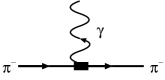
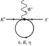
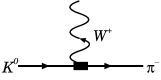
Figure 3: The NLO diagrams contributing to the pion
and the neutral kaon form factors.
The dark box is NLO vertex from ℒ ( 4 ) superscript ℒ 4 {\mathcal{L}}^{(4)}
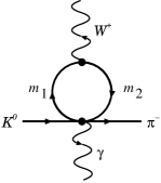
III.2 π K W 𝜋 𝐾 𝑊 \pi KW
The diagrams contributing to the NLO
π K W 𝜋 𝐾 𝑊 \pi KW 4 T ( c ) ( 4 ) subscript superscript 𝑇 4 𝑐 T^{(4)}_{(c)} T ( d ) ( 4 ) subscript superscript 𝑇 4 𝑑 T^{(4)}_{(d)}
T ( c ) ( 4 ) subscript superscript 𝑇 4 𝑐 \displaystyle T^{(4)}_{(c)} = \displaystyle= − G F 2 e 2 V u s ∗ 1 q 2 [ u ¯ ( k 2 ) { G 1 ( r c , l c ) ( p 1 + p 2 ) + G 2 ( r c , l c ) ( p 1 − p 2 ) } \displaystyle-\frac{G_{F}}{\sqrt{2}}e^{2}V_{us}^{*}\frac{1}{q^{2}}\bigg{[}\bar{u}(k_{2})\left\{G_{1}(r_{c},l_{c})(\not\!p_{1}+\not\!p_{2})+G_{2}(r_{c},l_{c})(\not\!p_{1}-\not\!p_{2})\right\} (21)
× ( 1 − γ 5 ) 2 k 1 μ + q γ μ ( k 1 + q ) 2 − m e 2 v ( k 1 ) ] u ¯ ( k 4 ) γ μ v ( k 3 ) , \displaystyle\times(1-\gamma_{5})\frac{2k_{1\mu}+\not\!q\gamma_{\mu}}{(k_{1}+q)^{2}-m_{e}^{2}}v(k_{1})\bigg{]}\bar{u}(k_{4})\gamma^{\mu}v(k_{3}),
T ( d ) ( 4 ) subscript superscript 𝑇 4 𝑑 \displaystyle T^{(4)}_{(d)} = \displaystyle= G F 2 e 2 V u s ∗ 1 q 2 [ u ¯ ( k 2 ) { G 1 ( r d , l d ) p 1 + p 2 + q ( p 2 + q ) 2 − m π 2 + G 2 ( r d , l d ) p 1 − p 2 − q ( p 2 + q ) 2 − m π 2 } \displaystyle\frac{G_{F}}{\sqrt{2}}e^{2}V_{us}^{*}\frac{1}{q^{2}}\bigg{[}\bar{u}(k_{2})\left\{G_{1}(r_{d},l_{d})\frac{\not\!p_{1}+\not\!p_{2}+\not\!q}{(p_{2}+q)^{2}-m_{\pi}^{2}}+G_{2}(r_{d},l_{d})\frac{\not\!p_{1}-\not\!p_{2}-\not\!q}{(p_{2}+q)^{2}-m_{\pi}^{2}}\right\} (22)
× ( 1 − γ 5 ) v ( k 1 ) ] u ¯ ( k 4 ) 2 p 2 v ( k 3 ) , \displaystyle\times(1-\gamma_{5})v(k_{1})\bigg{]}\bar{u}(k_{4})2\not\!p_{2}v(k_{3}),
with r c = p 1 + p 2 , l c = p 1 − p 2 , r d = p 1 + p 2 + q formulae-sequence subscript 𝑟 𝑐 subscript 𝑝 1 subscript 𝑝 2 formulae-sequence subscript 𝑙 𝑐 subscript 𝑝 1 subscript 𝑝 2 subscript 𝑟 𝑑 subscript 𝑝 1 subscript 𝑝 2 𝑞 r_{c}=p_{1}+p_{2},l_{c}=p_{1}-p_{2},r_{d}=p_{1}+p_{2}+q l d = p 1 − p 2 − q subscript 𝑙 𝑑 subscript 𝑝 1 subscript 𝑝 2 𝑞 l_{d}=p_{1}-p_{2}-q G 1 subscript 𝐺 1 G_{1} G 2 subscript 𝐺 2 G_{2} K π 𝐾 𝜋 K\pi
G 1 ( r , l ) subscript 𝐺 1 𝑟 𝑙 \displaystyle G_{1}(r,l) = \displaystyle= 2 L 9 F 0 2 l 2 + 3 8 F 0 2 { A ( m η 2 ) + A ( m π 2 ) + 2 A ( m K 2 ) } − 3 2 F 0 2 { B 22 ( m π 2 , m K 2 , l 2 ) + B 22 ( m K 2 , m η 2 , l 2 ) } , 2 subscript 𝐿 9 superscript subscript 𝐹 0 2 superscript 𝑙 2 3 8 superscript subscript 𝐹 0 2 𝐴 superscript subscript 𝑚 𝜂 2 𝐴 superscript subscript 𝑚 𝜋 2 2 𝐴 superscript subscript 𝑚 𝐾 2 3 2 superscript subscript 𝐹 0 2 subscript 𝐵 22 superscript subscript 𝑚 𝜋 2 superscript subscript 𝑚 𝐾 2 superscript 𝑙 2 subscript 𝐵 22 superscript subscript 𝑚 𝐾 2 superscript subscript 𝑚 𝜂 2 superscript 𝑙 2 \displaystyle\frac{2L_{9}}{F_{0}^{2}}l^{2}+\frac{3}{8F_{0}^{2}}\left\{A(m_{\eta}^{2})+A(m_{\pi}^{2})+2A(m_{K}^{2})\right\}-\frac{3}{2F_{0}^{2}}\left\{B_{22}(m_{\pi}^{2},m_{K}^{2},l^{2})+B_{22}(m_{K}^{2},m_{\eta}^{2},l^{2})\right\},
G 2 ( r , l ) subscript 𝐺 2 𝑟 𝑙 \displaystyle G_{2}(r,l) = \displaystyle= [ 4 ( m K 2 − m π 2 ) L 5 − 2 r ⋅ l L 9 + 1 2 A ( m η 2 ) − 5 12 A ( m π 2 ) + 7 12 A ( m K 2 ) \displaystyle\Big{[}4(m_{K}^{2}-m_{\pi}^{2})L_{5}-2r\cdot lL_{9}+\frac{1}{2}A(m_{\eta}^{2})-\frac{5}{12}A(m_{\pi}^{2})+\frac{7}{12}A(m_{K}^{2}) (24)
+ B ( m π 2 , m K 2 , l 2 ) { − 1 4 m π 2 + 1 6 m K 2 − 5 48 r 2 + 5 16 l 2 − 3 8 r ⋅ l } 𝐵 superscript subscript 𝑚 𝜋 2 superscript subscript 𝑚 𝐾 2 superscript 𝑙 2 1 4 superscript subscript 𝑚 𝜋 2 1 6 superscript subscript 𝑚 𝐾 2 5 48 superscript 𝑟 2 5 16 superscript 𝑙 2 ⋅ 3 8 𝑟 𝑙 \displaystyle\qquad+B(m_{\pi}^{2},m_{K}^{2},l^{2})\big{\{}-\frac{1}{4}m_{\pi}^{2}+\frac{1}{6}m_{K}^{2}-\frac{5}{48}r^{2}+\frac{5}{16}l^{2}-\frac{3}{8}r\cdot l\big{\}}
+ B ( m K , m η 2 , l 2 ) { − 1 6 m π 2 − 1 12 m K 2 − 1 16 r 2 + 3 16 l 2 − 3 8 r ⋅ l } 𝐵 subscript 𝑚 𝐾 superscript subscript 𝑚 𝜂 2 superscript 𝑙 2 1 6 superscript subscript 𝑚 𝜋 2 1 12 superscript subscript 𝑚 𝐾 2 1 16 superscript 𝑟 2 3 16 superscript 𝑙 2 ⋅ 3 8 𝑟 𝑙 \displaystyle\qquad+B(m_{K},m_{\eta}^{2},l^{2})\big{\{}-\frac{1}{6}m_{\pi}^{2}-\frac{1}{12}m_{K}^{2}-\frac{1}{16}r^{2}+\frac{3}{16}l^{2}-\frac{3}{8}r\cdot l\big{\}}
+ B 1 ( m π 2 , m K 2 , l 2 ) { 1 2 m π 2 − 1 3 m K 2 + 5 24 r 2 − 5 24 l 2 + 3 2 r ⋅ l } subscript 𝐵 1 superscript subscript 𝑚 𝜋 2 superscript subscript 𝑚 𝐾 2 superscript 𝑙 2 1 2 superscript subscript 𝑚 𝜋 2 1 3 superscript subscript 𝑚 𝐾 2 5 24 superscript 𝑟 2 5 24 superscript 𝑙 2 ⋅ 3 2 𝑟 𝑙 \displaystyle\qquad+B_{1}(m_{\pi}^{2},m_{K}^{2},l^{2})\big{\{}\frac{1}{2}m_{\pi}^{2}-\frac{1}{3}m_{K}^{2}+\frac{5}{24}r^{2}-\frac{5}{24}l^{2}+\frac{3}{2}r\cdot l\big{\}}
+ B 1 ( m K , m η 2 , l 2 ) { 1 3 m π 2 + 1 6 m K 2 + 1 8 r 2 − 1 8 l 2 + 3 2 r ⋅ l } subscript 𝐵 1 subscript 𝑚 𝐾 superscript subscript 𝑚 𝜂 2 superscript 𝑙 2 1 3 superscript subscript 𝑚 𝜋 2 1 6 superscript subscript 𝑚 𝐾 2 1 8 superscript 𝑟 2 1 8 superscript 𝑙 2 ⋅ 3 2 𝑟 𝑙 \displaystyle\qquad+B_{1}(m_{K},m_{\eta}^{2},l^{2})\big{\{}\frac{1}{3}m_{\pi}^{2}+\frac{1}{6}m_{K}^{2}+\frac{1}{8}r^{2}-\frac{1}{8}l^{2}+\frac{3}{2}r\cdot l\big{\}}
+ B 21 ( m π 2 , m K 2 , l 2 ) { − 5 6 l 2 − 3 2 r ⋅ l } + B ( m K , m η 2 , l 2 ) { − 3 2 r ⋅ l − 1 2 l 2 } subscript 𝐵 21 superscript subscript 𝑚 𝜋 2 superscript subscript 𝑚 𝐾 2 superscript 𝑙 2 5 6 superscript 𝑙 2 ⋅ 3 2 𝑟 𝑙 𝐵 subscript 𝑚 𝐾 superscript subscript 𝑚 𝜂 2 superscript 𝑙 2 ⋅ 3 2 𝑟 𝑙 1 2 superscript 𝑙 2 \displaystyle\qquad+B_{21}(m_{\pi}^{2},m_{K}^{2},l^{2})\big{\{}-\frac{5}{6}l^{2}-\frac{3}{2}r\cdot l\big{\}}+B(m_{K},m_{\eta}^{2},l^{2})\big{\{}-\frac{3}{2}r\cdot l-\frac{1}{2}l^{2}\big{\}}
− 5 6 B 22 ( m π 2 , m K 2 , l 2 ) − 1 2 B 22 ( m K 2 , m η 2 , l 2 ) ] 1 F 0 2 . \displaystyle\qquad-\frac{5}{6}B_{22}(m_{\pi}^{2},m_{K}^{2},l^{2})-\frac{1}{2}B_{22}(m_{K}^{2},m_{\eta}^{2},l^{2})\Big{]}\frac{1}{F_{0}^{2}}.
Those expressions agree with Eqs. (4.3)-(4.4) of bijn1
Figure 4: The NLO diagrams contributing to
π K W 𝜋 𝐾 𝑊 \pi KW ( m 1 , m 2 ) subscript 𝑚 1 subscript 𝑚 2 (m_{1},m_{2}) ( K + , η ) superscript 𝐾 𝜂 (K^{+},\eta) ( π + , K 0 ) superscript 𝜋 superscript 𝐾 0 (\pi^{+},K^{0}) ( K + , π 0 ) superscript 𝐾 superscript 𝜋 0 (K^{+},\pi^{0})
III.3 π K W γ 𝜋 𝐾 𝑊 𝛾 \pi KW\gamma
The amplitude with the NLO correction of π K W γ 𝜋 𝐾 𝑊 𝛾 \pi KW\gamma
T ( e ) ( 4 ) subscript superscript 𝑇 4 𝑒 \displaystyle T^{(4)}_{(e)} = \displaystyle= − G F 2 e 2 V u s ∗ 1 q 2 u ¯ ( k 2 ) γ ν ( 1 − γ 5 ) v ( k 1 ) u ¯ ( k 4 ) γ μ v ( k 3 ) ∑ α = a f t ( α ) μ ν 1 F 0 2 . subscript 𝐺 𝐹 2 superscript 𝑒 2 superscript subscript 𝑉 𝑢 𝑠 1 superscript 𝑞 2 ¯ 𝑢 subscript 𝑘 2 subscript 𝛾 𝜈 1 subscript 𝛾 5 𝑣 subscript 𝑘 1 ¯ 𝑢 subscript 𝑘 4 subscript 𝛾 𝜇 𝑣 subscript 𝑘 3 superscript subscript 𝛼 𝑎 𝑓 subscript superscript 𝑡 𝜇 𝜈 𝛼 1 superscript subscript 𝐹 0 2 \displaystyle-\frac{G_{F}}{\sqrt{2}}e^{2}V_{us}^{*}\frac{1}{q^{2}}\bar{u}(k_{2})\gamma_{\nu}(1-\gamma_{5})v(k_{1})\bar{u}(k_{4})\gamma_{\mu}v(k_{3})\sum_{\alpha=a}^{f}t^{\mu\nu}_{(\alpha)}\frac{1}{F_{0}^{2}}. (25)
The local interaction ℒ ( 4 ) superscript ℒ 4 \mathcal{L}^{(4)} 5
t ( a ) μ ν subscript superscript 𝑡 𝜇 𝜈 𝑎 \displaystyle t^{\mu\nu}_{(a)} = \displaystyle= [ − 1 8 A ( m η 2 ) − 11 24 A ( m π 2 ) − 5 12 A ( m K 2 ) + 4 ( m π 2 − m K 2 ) L 5 + 4 L 9 ( W ⋅ p 1 − q ⋅ p 2 ) \displaystyle\ \Big{[}-\frac{1}{8}A(m_{\eta}^{2})-\frac{11}{24}A(m_{\pi}^{2})-\frac{5}{12}A(m_{K}^{2})+4(m_{\pi}^{2}-m_{K}^{2})L_{5}+4L_{9}(W\cdot p_{1}-q\cdot p_{2}) (26)
+ 4 L 10 W ⋅ q ] g μ ν + L 9 [ − 4 W μ W ν − 8 W μ p 2 ν + 8 p 2 μ q ν + 4 p 2 μ W ν − 4 q μ p 2 ν ] \displaystyle+4L_{10}W\cdot q\Big{]}g^{\mu\nu}+L_{9}\Big{[}-4W^{\mu}W^{\nu}-8W^{\mu}p_{2}^{\nu}+8p_{2}^{\mu}q^{\nu}+4p_{2}^{\mu}W^{\nu}-4q^{\mu}p_{2}^{\nu}\Big{]}
− 4 [ L 9 + L 10 ] W μ q ν . 4 delimited-[] subscript 𝐿 9 subscript 𝐿 10 superscript 𝑊 𝜇 superscript 𝑞 𝜈 \displaystyle-4\left[L_{9}+L_{10}\right]W^{\mu}q^{\nu}.
Here q μ superscript 𝑞 𝜇 q^{\mu} W μ superscript 𝑊 𝜇 W^{\mu} q μ = k 3 μ + k 4 μ superscript 𝑞 𝜇 superscript subscript 𝑘 3 𝜇 superscript subscript 𝑘 4 𝜇 q^{\mu}=k_{3}^{\mu}+k_{4}^{\mu} W μ = k 1 μ + k 2 μ superscript 𝑊 𝜇 superscript subscript 𝑘 1 𝜇 superscript subscript 𝑘 2 𝜇 W^{\mu}=k_{1}^{\mu}+k_{2}^{\mu}
The contributions of the loop diagrams shown in
Fig. 5 5
t ( b ) μ ν subscript superscript 𝑡 𝜇 𝜈 𝑏 \displaystyle t^{\mu\nu}_{(b)} = \displaystyle= [ 35 12 A ( m π 2 ) + 1 4 A ( m η 2 ) + A ( m K 2 ) ] g μ ν , delimited-[] 35 12 𝐴 superscript subscript 𝑚 𝜋 2 1 4 𝐴 superscript subscript 𝑚 𝜂 2 𝐴 superscript subscript 𝑚 𝐾 2 superscript 𝑔 𝜇 𝜈 \displaystyle\left[\frac{35}{12}A(m_{\pi}^{2})+\frac{1}{4}A(m_{\eta}^{2})+A(m_{K}^{2})\right]g^{\mu\nu}, (27)
t ( c ) μ ν subscript superscript 𝑡 𝜇 𝜈 𝑐 \displaystyle t^{\mu\nu}_{(c)} = \displaystyle= − 10 3 B 22 ( m π 2 , m π 2 , q 2 ) g μ ν , 10 3 subscript 𝐵 22 superscript subscript 𝑚 𝜋 2 superscript subscript 𝑚 𝜋 2 superscript 𝑞 2 superscript 𝑔 𝜇 𝜈 \displaystyle-\frac{10}{3}B_{22}(m_{\pi}^{2},m_{\pi}^{2},q^{2})g^{\mu\nu}, (28)
t ( d ) μ ν subscript superscript 𝑡 𝜇 𝜈 𝑑 \displaystyle t^{\mu\nu}_{(d)} = \displaystyle= [ − 1 4 A ( m K 2 ) − 2 B 22 ( m K 2 , m η 2 , W 2 ) − 4 3 B 22 ( m π 2 , m K 2 , W 2 ) ] g μ ν delimited-[] 1 4 𝐴 superscript subscript 𝑚 𝐾 2 2 subscript 𝐵 22 superscript subscript 𝑚 𝐾 2 superscript subscript 𝑚 𝜂 2 superscript 𝑊 2 4 3 subscript 𝐵 22 superscript subscript 𝑚 𝜋 2 superscript subscript 𝑚 𝐾 2 superscript 𝑊 2 superscript 𝑔 𝜇 𝜈 \displaystyle\Bigg{[}-\frac{1}{4}A(m_{K}^{2})-2B_{22}(m_{K}^{2},m_{\eta}^{2},W^{2})-\frac{4}{3}B_{22}(m_{\pi}^{2},m_{K}^{2},W^{2})\Bigg{]}g^{\mu\nu} (29)
+ \displaystyle+ [ − 2 B 21 ( m K 2 , m η 2 , W 2 ) + 1 2 B ( m K 2 , m π 2 , W 2 ) − B 1 ( m K 2 , m π 2 , W 2 ) − 4 3 B 21 ( m π 2 , m K 2 , W 2 ) ] W μ W ν delimited-[] 2 subscript 𝐵 21 superscript subscript 𝑚 𝐾 2 superscript subscript 𝑚 𝜂 2 superscript 𝑊 2 1 2 𝐵 superscript subscript 𝑚 𝐾 2 subscript superscript 𝑚 2 𝜋 superscript 𝑊 2 subscript 𝐵 1 superscript subscript 𝑚 𝐾 2 subscript superscript 𝑚 2 𝜋 superscript 𝑊 2 4 3 subscript 𝐵 21 superscript subscript 𝑚 𝜋 2 superscript subscript 𝑚 𝐾 2 superscript 𝑊 2 superscript 𝑊 𝜇 superscript 𝑊 𝜈 \displaystyle\Bigg{[}-2B_{21}(m_{K}^{2},m_{\eta}^{2},W^{2})+\frac{1}{2}B(m_{K}^{2},m^{2}_{\pi},W^{2})-B_{1}(m_{K}^{2},m^{2}_{\pi},W^{2})-\frac{4}{3}B_{21}(m_{\pi}^{2},m_{K}^{2},W^{2})\Bigg{]}W^{\mu}W^{\nu}
+ \displaystyle+ [ 2 B 1 ( m K 2 , m η 2 , W 2 ) + 4 3 B 1 ( m π 2 , m K 2 , W 2 ) ] ( p 2 μ + 2 W μ ) W ν delimited-[] 2 subscript 𝐵 1 superscript subscript 𝑚 𝐾 2 superscript subscript 𝑚 𝜂 2 superscript 𝑊 2 4 3 subscript 𝐵 1 superscript subscript 𝑚 𝜋 2 superscript subscript 𝑚 𝐾 2 superscript 𝑊 2 superscript subscript 𝑝 2 𝜇 2 superscript 𝑊 𝜇 superscript 𝑊 𝜈 \displaystyle\Bigg{[}2B_{1}(m_{K}^{2},m_{\eta}^{2},W^{2})+\frac{4}{3}B_{1}(m_{\pi}^{2},m_{K}^{2},W^{2})\Bigg{]}(p_{2}^{\mu}+2W^{\mu})W^{\nu}
+ \displaystyle+ [ − 1 2 B ( m K 2 , m η 2 , W 2 ) − 1 3 B ( m π 2 , m K 2 , W 2 ) ] ( 2 p 2 μ + 3 W μ ) W ν , delimited-[] 1 2 𝐵 superscript subscript 𝑚 𝐾 2 superscript subscript 𝑚 𝜂 2 superscript 𝑊 2 1 3 𝐵 superscript subscript 𝑚 𝜋 2 superscript subscript 𝑚 𝐾 2 superscript 𝑊 2 2 superscript subscript 𝑝 2 𝜇 3 superscript 𝑊 𝜇 superscript 𝑊 𝜈 \displaystyle\Bigg{[}-\frac{1}{2}B(m_{K}^{2},m_{\eta}^{2},W^{2})-\frac{1}{3}B(m_{\pi}^{2},m_{K}^{2},W^{2})\Bigg{]}(2p_{2}^{\mu}+3W^{\mu})W^{\nu},
t ( e ) μ ν subscript superscript 𝑡 𝜇 𝜈 𝑒 \displaystyle t^{\mu\nu}_{(e)} = \displaystyle= [ 1 2 ( 3 p 2 + Q ) ⋅ Q B 1 ( m K 2 , m η 2 , Q 2 ) − { p 2 ⋅ Q + 1 6 ( m K 2 + 2 m π 2 ) } B ( m K 2 , m η 2 , Q 2 ) \displaystyle\Bigg{[}\frac{1}{2}(3p_{2}+Q)\cdot QB_{1}(m_{K}^{2},m_{\eta}^{2},Q^{2})-\left\{p_{2}\cdot Q+\frac{1}{6}(m_{K}^{2}+2m_{\pi}^{2})\right\}B(m_{K}^{2},m_{\eta}^{2},Q^{2}) (30)
+ \displaystyle+ 1 4 A ( m K 2 ) − 1 6 A ( m π 2 ) + ( 1 2 p 1 + p 2 + 1 3 Q ) ⋅ Q B 1 ( m π 2 , m K 2 , Q 2 ) 1 4 𝐴 superscript subscript 𝑚 𝐾 2 1 6 𝐴 superscript subscript 𝑚 𝜋 2 ⋅ 1 2 subscript 𝑝 1 subscript 𝑝 2 1 3 𝑄 𝑄 subscript 𝐵 1 superscript subscript 𝑚 𝜋 2 superscript subscript 𝑚 𝐾 2 superscript 𝑄 2 \displaystyle\frac{1}{4}A(m_{K}^{2})-\frac{1}{6}A(m_{\pi}^{2})+(\frac{1}{2}p_{1}+p_{2}+\frac{1}{3}Q)\cdot QB_{1}(m_{\pi}^{2},m_{K}^{2},Q^{2})
+ \displaystyle+ ( 1 2 ( m π 2 − Q 2 ) − 2 3 p 2 ⋅ Q ) B ( m π 2 , m K 2 , Q 2 ) ] g μ ν , \displaystyle(\frac{1}{2}(m_{\pi}^{2}-Q^{2})-\frac{2}{3}p_{2}\cdot Q)B(m_{\pi}^{2},m_{K}^{2},Q^{2})\Bigg{]}g^{\mu\nu},
t ( f ) μ ν subscript superscript 𝑡 𝜇 𝜈 𝑓 \displaystyle t^{\mu\nu}_{(f)} = \displaystyle= t ~ K K η μ ν + t ~ K K π μ ν + 2 3 [ g μ ν B 22 ( m π 2 , m π 2 , q 2 ) + t ~ π π K μ ν ] . subscript superscript ~ 𝑡 𝜇 𝜈 𝐾 𝐾 𝜂 subscript superscript ~ 𝑡 𝜇 𝜈 𝐾 𝐾 𝜋 2 3 delimited-[] superscript 𝑔 𝜇 𝜈 subscript 𝐵 22 superscript subscript 𝑚 𝜋 2 superscript subscript 𝑚 𝜋 2 superscript 𝑞 2 subscript superscript ~ 𝑡 𝜇 𝜈 𝜋 𝜋 𝐾 \displaystyle\tilde{t}^{\mu\nu}_{KK\eta}+\tilde{t}^{\mu\nu}_{KK\pi}+\frac{2}{3}[g^{\mu\nu}B_{22}(m_{\pi}^{2},m_{\pi}^{2},q^{2})+\tilde{t}^{\mu\nu}_{\pi\pi K}]. (31)
Here Q μ = q μ + W μ superscript 𝑄 𝜇 superscript 𝑞 𝜇 superscript 𝑊 𝜇 Q^{\mu}=q^{\mu}+W^{\mu} t ~ β μ ν subscript superscript ~ 𝑡 𝜇 𝜈 𝛽 \tilde{t}^{\mu\nu}_{\beta} β = K K η , K K π , π π K 𝛽 𝐾 𝐾 𝜂 𝐾 𝐾 𝜋 𝜋 𝜋 𝐾
\beta=KK\eta,KK\pi,\pi\pi K
t ~ β μ ν subscript superscript ~ 𝑡 𝜇 𝜈 𝛽 \displaystyle\tilde{t}^{\mu\nu}_{\beta} = \displaystyle= − g μ ν [ a β C 001 ( β ) + b β C 002 ( β ) + c β C 00 ( β ) ] + p 2 μ q ν d β [ C 00 ( β ) − C 001 ( β ) − C 002 ( β ) ] superscript 𝑔 𝜇 𝜈 delimited-[] subscript 𝑎 𝛽 subscript 𝐶 001 𝛽 subscript 𝑏 𝛽 subscript 𝐶 002 𝛽 subscript 𝑐 𝛽 subscript 𝐶 00 𝛽 superscript subscript 𝑝 2 𝜇 superscript 𝑞 𝜈 subscript 𝑑 𝛽 delimited-[] subscript 𝐶 00 𝛽 subscript 𝐶 001 𝛽 subscript 𝐶 002 𝛽 \displaystyle-g^{\mu\nu}\left[\,a_{\beta}C_{001}(\beta)+b_{\beta}C_{002}(\beta)+c_{\beta}C_{00}(\beta)\,\right]+p_{2}^{\mu}q^{\nu}d_{\beta}\left[\,C_{00}(\beta)-C_{001}(\beta)-C_{002}(\beta)\,\right] (32)
+ \displaystyle+ W μ q ν [ − 2 C 001 ( β ) − 4 C 002 ( β ) − a β C 112 ( β ) − ( a β + b β ) C 122 ( β ) \displaystyle W^{\mu}q^{\nu}\bigg{[}-2C_{001}(\beta)-4C_{002}(\beta)-a_{\beta}C_{112}(\beta)-(a_{\beta}+b_{\beta})C_{122}(\beta)
− b β C 222 ( β ) + ( b β − c β ) C 22 ( β ) + ( a β − c β ) C 12 ( β ) + 2 C 00 ( β ) + c β C 2 ( β ) ] \displaystyle-b_{\beta}C_{222}(\beta)+(b_{\beta}-c_{\beta})C_{22}(\beta)+(a_{\beta}-c_{\beta})C_{12}(\beta)+2C_{00}(\beta)+c_{\beta}C_{2}(\beta)\,\bigg{]}
+ \displaystyle+ W μ W ν [ − 4 C 002 ( β ) − a β C 122 ( β ) − b β C 222 ( β ) + { 1 2 b β − c β } C 22 ( β ) \displaystyle W^{\mu}W^{\nu}\bigg{[}-4C_{002}(\beta)-a_{\beta}C_{122}(\beta)-b_{\beta}C_{222}(\beta)+\left\{\frac{1}{2}b_{\beta}-c_{\beta}\right\}C_{22}(\beta)
+ 1 2 a β C 12 ( β ) + C 00 ( β ) + 1 2 c β C 2 ( β ) ] \displaystyle+\frac{1}{2}a_{\beta}C_{12}(\beta)+C_{00}(\beta)+\frac{1}{2}c_{\beta}C_{2}(\beta)\,\bigg{]}
− \displaystyle- W μ p 2 ν d β C 002 ( β ) + p 2 μ W ν d β [ − C 002 ( β ) + 1 2 C 00 ( β ) ] . superscript 𝑊 𝜇 superscript subscript 𝑝 2 𝜈 subscript 𝑑 𝛽 subscript 𝐶 002 𝛽 superscript subscript 𝑝 2 𝜇 superscript 𝑊 𝜈 subscript 𝑑 𝛽 delimited-[] subscript 𝐶 002 𝛽 1 2 subscript 𝐶 00 𝛽 \displaystyle W^{\mu}p_{2}^{\nu}d_{\beta}C_{002}(\beta)+p_{2}^{\mu}W^{\nu}d_{\beta}\left[\,-C_{002}(\beta)+\frac{1}{2}C_{00}(\beta)\,\right].
The coefficients a β , b β , c β , d β subscript 𝑎 𝛽 subscript 𝑏 𝛽 subscript 𝑐 𝛽 subscript 𝑑 𝛽
a_{\beta},b_{\beta},c_{\beta},d_{\beta} m 1 2 , m 2 2 , m 3 2 superscript subscript 𝑚 1 2 superscript subscript 𝑚 2 2 superscript subscript 𝑚 3 2
m_{1}^{2},m_{2}^{2},m_{3}^{2} C 2 , C i j , C i j k subscript 𝐶 2 subscript 𝐶 𝑖 𝑗 subscript 𝐶 𝑖 𝑗 𝑘
C_{2},C_{ij},C_{ijk}
Table 1: Coefficients a β , b β , c β , d β subscript 𝑎 𝛽 subscript 𝑏 𝛽 subscript 𝑐 𝛽 subscript 𝑑 𝛽
a_{\beta},b_{\beta},c_{\beta},d_{\beta} C 2 , C i j , C i j k subscript 𝐶 2 subscript 𝐶 𝑖 𝑗 subscript 𝐶 𝑖 𝑗 𝑘
C_{2},C_{ij},C_{ijk}
Figure 5: The NLO diagrams contributing to π K W γ 𝜋 𝐾 𝑊 𝛾 \pi KW\gamma ( m 1 , m 2 ) subscript 𝑚 1 subscript 𝑚 2 (m_{1},m_{2}) ( K + , η ) superscript 𝐾 𝜂 (K^{+},\eta) ( π + , K 0 ) superscript 𝜋 superscript 𝐾 0 (\pi^{+},K^{0}) ( K + , π 0 ) superscript 𝐾 superscript 𝜋 0 (K^{+},\pi^{0})
III.4 Chiral anomaly term
Finally the contribution of the
chiral anomaly term T ( e , a n o m ) ( 4 ) subscript superscript 𝑇 4 𝑒 𝑎 𝑛 𝑜 𝑚 T^{(4)}_{(e,anom)}
T ( e , a n o m ) ( 4 ) = − G F 2 e 2 V u s ∗ 1 q 2 ( − i 8 π 2 F 0 2 ) ϵ μ ν ρ σ q ρ W σ u ¯ ( k 2 ) γ ν ( 1 − γ 5 ) v ( k 1 ) u ¯ ( k 4 ) γ μ v ( k 3 ) . subscript superscript 𝑇 4 𝑒 𝑎 𝑛 𝑜 𝑚 subscript 𝐺 𝐹 2 superscript 𝑒 2 superscript subscript 𝑉 𝑢 𝑠 1 superscript 𝑞 2 𝑖 8 superscript 𝜋 2 superscript subscript 𝐹 0 2 superscript italic-ϵ 𝜇 𝜈 𝜌 𝜎 subscript 𝑞 𝜌 subscript 𝑊 𝜎 ¯ 𝑢 subscript 𝑘 2 subscript 𝛾 𝜈 1 subscript 𝛾 5 𝑣 subscript 𝑘 1 ¯ 𝑢 subscript 𝑘 4 subscript 𝛾 𝜇 𝑣 subscript 𝑘 3 T^{(4)}_{(e,anom)}=-\frac{G_{F}}{\sqrt{2}}e^{2}V_{us}^{*}\frac{1}{q^{2}}\left(-\frac{i}{8\pi^{2}F_{0}^{2}}\right)\epsilon^{\mu\nu\rho\sigma}q_{\rho}W_{\sigma}\bar{u}(k_{2})\gamma_{\nu}(1-\gamma_{5})v(k_{1})\bar{u}(k_{4})\gamma_{\mu}v(k_{3}). (33)
IV Results and Discussions
The total decay rate of K e 3 e + e − 0 subscript superscript 𝐾 0 𝑒 3 superscript 𝑒 superscript 𝑒 K^{0}_{e3e^{+}e^{-}}
Γ ( K e 3 e + e − 0 ) = 1 2 m K ( 2 π ) 11 ∫ d 𝒑 2 2 p 2 0 ∫ d 𝒌 1 2 k 1 0 ⋯ ∫ d 𝒌 4 2 k 4 0 δ 4 ( p i − p f ) ∑ f | T f i | 2 . Γ subscript superscript 𝐾 0 𝑒 3 superscript 𝑒 superscript 𝑒 1 2 subscript 𝑚 𝐾 superscript 2 𝜋 11 𝑑 subscript 𝒑 2 2 superscript subscript 𝑝 2 0 𝑑 subscript 𝒌 1 2 superscript subscript 𝑘 1 0 ⋯ 𝑑 subscript 𝒌 4 2 superscript subscript 𝑘 4 0 superscript 𝛿 4 subscript 𝑝 𝑖 subscript 𝑝 𝑓 subscript 𝑓 superscript subscript 𝑇 𝑓 𝑖 2 \displaystyle\Gamma(K^{0}_{e3e^{+}e^{-}})=\frac{1}{2m_{K}(2\pi)^{11}}\int\,\frac{d{\bm{p}}_{2}}{2p_{2}^{0}}\,\int\,\frac{d{\bm{k}}_{1}}{2k_{1}^{0}}\,\cdots\int\,\frac{d{\bm{k}}_{4}}{2k_{4}^{0}}\,\delta^{4}\left(p_{i}-p_{f}\right)\sum_{f}|T_{fi}|^{2}. (34)
The transition matrix element T f i subscript 𝑇 𝑓 𝑖 T_{fi} T ( 2 ) superscript 𝑇 2 T^{(2)} T ( 4 ) superscript 𝑇 4 T^{(4)}
The multi-dimensional phase space integration is performed by using
the Vegas integration lepage T ( 4 ) superscript 𝑇 4 T^{(4)} Looptoolshahn ; oldenborgh . In the following results,
we use the masses of the neutral kaon and the charged pion and the charged pion
decay constant pdg
m K = 497.67 MeV , m π = 139.57 MeV , F π = 92.4 MeV . formulae-sequence subscript 𝑚 𝐾 497.67 MeV formulae-sequence subscript 𝑚 𝜋 139.57 MeV subscript 𝐹 𝜋 92.4 MeV m_{K}=497.67\;\textrm{MeV},\quad m_{\pi}=139.57\;\textrm{MeV},\quad F_{\pi}=92.4\;\textrm{MeV}. (35)
We use the following low energy constants at the scale of μ = m ρ = 770 𝜇 subscript 𝑚 𝜌 770 \mu=m_{\rho}=770 bijnens-3
L 9 r ( m ρ ) = 6.9 × 10 − 3 , L 10 r ( m ρ ) = − 5.5 × 10 − 3 formulae-sequence superscript subscript 𝐿 9 𝑟 subscript 𝑚 𝜌 6.9 superscript 10 3 superscript subscript 𝐿 10 𝑟 subscript 𝑚 𝜌 5.5 superscript 10 3 L_{9}^{r}(m_{\rho})=6.9\times 10^{-3},\quad L_{10}^{r}(m_{\rho})=-5.5\times 10^{-3}\quad (36)
and we use F K / F π = 1.22 subscript 𝐹 𝐾 subscript 𝐹 𝜋 1.22 F_{K}/F_{\pi}=1.22 L 5 subscript 𝐿 5 L_{5} | V u s | = 0.220 subscript 𝑉 𝑢 𝑠 0.220 |V_{us}|=0.220 pdg G F = 1.16637 × 10 − 5 G e V − 2 subscript 𝐺 𝐹 1.16637 superscript 10 5 𝐺 𝑒 superscript 𝑉 2 G_{F}=1.16637\times 10^{-5}GeV^{-2}
The role of the 𝒪 ( p 4 ) 𝒪 superscript 𝑝 4 {\mathcal{O}}(p^{4}) K e 3 e + e − 0 subscript superscript 𝐾 0 𝑒 3 superscript 𝑒 superscript 𝑒 K^{0}_{e3e^{+}e^{-}} d Γ / d E ν 𝑑 Γ 𝑑 subscript 𝐸 𝜈 d\Gamma/dE_{\nu} e + e − e + ν e superscript 𝑒 superscript 𝑒 superscript 𝑒 subscript 𝜈 𝑒 e^{+}e^{-}e^{+}\nu_{e} d Γ / d M 3 e ν 𝑑 Γ 𝑑 subscript 𝑀 3 𝑒 𝜈 d\Gamma/dM_{3e\nu} M 3 e ν = ( k 1 + k 2 + k 3 + k 4 ) 2 = ( p 1 − p 2 ) 2 subscript 𝑀 3 𝑒 𝜈 superscript subscript 𝑘 1 subscript 𝑘 2 subscript 𝑘 3 subscript 𝑘 4 2 superscript subscript 𝑝 1 subscript 𝑝 2 2 M_{3e\nu}=\sqrt{(k_{1}+k_{2}+k_{3}+k_{4})^{2}}=\sqrt{(p_{1}-p_{2})^{2}} e + e − superscript 𝑒 superscript 𝑒 e^{+}e^{-} d Γ / d M e + e − 𝑑 Γ 𝑑 subscript 𝑀 superscript 𝑒 superscript 𝑒 d\Gamma/dM_{e^{+}e^{-}} M e + e − = q 2 subscript 𝑀 superscript 𝑒 superscript 𝑒 superscript 𝑞 2 M_{e^{+}e^{-}}=\sqrt{q^{2}} q 2 superscript 𝑞 2 q^{2} K l 3 γ 0 subscript superscript 𝐾 0 𝑙 3 𝛾 K^{0}_{l3\gamma} d Γ / d M 3 e ν e 𝑑 Γ 𝑑 subscript 𝑀 3 𝑒 subscript 𝜈 𝑒 d\Gamma/dM_{3e\nu_{e}} d Γ / E ν 𝑑 Γ subscript 𝐸 𝜈 d\Gamma/E_{\nu} d Γ / M e + e − 𝑑 Γ subscript 𝑀 superscript 𝑒 superscript 𝑒 d\Gamma/M_{e^{+}e^{-}} 6 𝒪 ( p 2 ) 𝒪 superscript 𝑝 2 {\mathcal{O}}(p^{2}) 𝒪 ( p 2 ) + 𝒪 ( p 4 ) 𝒪 superscript 𝑝 2 𝒪 superscript 𝑝 4 {\mathcal{O}}(p^{2})+{\mathcal{O}}(p^{4}) LABEL:leading ) in the LO amplitude plays a dominant
role. Around the peak of those distributions, effects of the
𝒪 ( p 4 ) 𝒪 superscript 𝑝 4 {\mathcal{O}}(p^{4}) M 3 e ν e subscript 𝑀 3 𝑒 subscript 𝜈 𝑒 M_{3e\nu_{e}} E ν subscript 𝐸 𝜈 E_{\nu} M e + e − subscript 𝑀 superscript 𝑒 superscript 𝑒 M_{e^{+}e^{-}}
The effect of the 𝒪 ( p 4 ) 𝒪 superscript 𝑝 4 {\mathcal{O}}(p^{4}) d Γ ( L O + N L O ) / d Γ ( L O ) 𝑑 Γ 𝐿 𝑂 𝑁 𝐿 𝑂 𝑑 Γ 𝐿 𝑂 d\Gamma(LO+NLO)/d\Gamma(LO) 7 𝒪 ( p 4 ) 𝒪 superscript 𝑝 4 {\mathcal{O}}(p^{4}) 𝒪 ( p 4 ) 𝒪 superscript 𝑝 4 {\mathcal{O}}(p^{4}) L 5 = L 10 = 0 subscript 𝐿 5 subscript 𝐿 10 0 L_{5}=L_{10}=0 L 9 subscript 𝐿 9 L_{9} 𝒪 ( p 4 ) 𝒪 superscript 𝑝 4 {\mathcal{O}}(p^{4}) M 3 e ν e subscript 𝑀 3 𝑒 subscript 𝜈 𝑒 M_{3e\nu_{e}} M 3 e ν e > 200 subscript 𝑀 3 𝑒 subscript 𝜈 𝑒 200 M_{3e\nu_{e}}>200 E ν subscript 𝐸 𝜈 E_{\nu} M 3 e ν e subscript 𝑀 3 𝑒 subscript 𝜈 𝑒 M_{3e\nu_{e}} E ν subscript 𝐸 𝜈 E_{\nu} 𝒪 ( p 4 ) 𝒪 superscript 𝑝 4 {\mathcal{O}}(p^{4}) L 9 subscript 𝐿 9 L_{9} L 5 subscript 𝐿 5 L_{5} L 10 subscript 𝐿 10 L_{10} M 3 e ν e subscript 𝑀 3 𝑒 subscript 𝜈 𝑒 M_{3e\nu_{e}} E ν subscript 𝐸 𝜈 E_{\nu} M e + e − subscript 𝑀 superscript 𝑒 superscript 𝑒 M_{e^{+}e^{-}} 𝒪 ( p 4 ) 𝒪 superscript 𝑝 4 {\mathcal{O}}(p^{4}) L 9 subscript 𝐿 9 L_{9} M e + e − subscript 𝑀 superscript 𝑒 superscript 𝑒 M_{e^{+}e^{-}} M e + e − = 100 subscript 𝑀 superscript 𝑒 superscript 𝑒 100 M_{e^{+}e^{-}}=100 L 10 subscript 𝐿 10 L_{10} L 9 subscript 𝐿 9 L_{9} ϵ μ ν ρ σ q ρ W σ superscript italic-ϵ 𝜇 𝜈 𝜌 𝜎 subscript 𝑞 𝜌 subscript 𝑊 𝜎 \epsilon^{\mu\nu\rho\sigma}q_{\rho}W_{\sigma} M e + e − = q 2 subscript 𝑀 superscript 𝑒 superscript 𝑒 superscript 𝑞 2 M_{e^{+}e^{-}}=\sqrt{q^{2}} M e + e − = 150 ∼ 200 subscript 𝑀 superscript 𝑒 superscript 𝑒 150 similar-to 200 M_{e^{+}e^{-}}=150\sim 200 M e + e − subscript 𝑀 superscript 𝑒 superscript 𝑒 M_{e^{+}e^{-}} q 2 superscript 𝑞 2 q^{2} M e + e − subscript 𝑀 superscript 𝑒 superscript 𝑒 M_{e^{+}e^{-}} K μ 3 e + e − 0 subscript superscript 𝐾 0 𝜇 3 superscript 𝑒 superscript 𝑒 K^{0}_{\mu 3e^{+}e^{-}}
Finally we examine
the total decay rate of K l 3 e + e − 0 ( l = e , μ ) subscript superscript 𝐾 0 𝑙 3 superscript 𝑒 superscript 𝑒 𝑙 𝑒 𝜇
K^{0}_{l3e^{+}e^{-}}(l=e,\mu) K l 3 0 subscript superscript 𝐾 0 𝑙 3 K^{0}_{l3}
ℛ ( K l 3 e + e − 0 ) = Γ ( K l 3 e + e − 0 ) Γ ( K l 3 0 ) . ( l = e , μ ) \displaystyle{\mathcal{R}}(K^{0}_{l3e^{+}e^{-}})=\frac{\Gamma(K^{0}_{l3e^{+}e^{-}})}{\Gamma(K^{0}_{l3})}.\quad(l=e,\mu) (37)
The decay rate Γ ( K l 3 0 ) Γ subscript superscript 𝐾 0 𝑙 3 \Gamma(K^{0}_{l3}) 𝒪 ( p 4 ) 𝒪 superscript 𝑝 4 {\mathcal{O}}(p^{4}) gasser-2 ℛ ℛ {\mathcal{R}} 2 𝒪 ( p 4 ) 𝒪 superscript 𝑝 4 {\mathcal{O}}(p^{4}) 𝒪 ( p 2 ) 𝒪 superscript 𝑝 2 {\mathcal{O}}(p^{2}) L i r = 0 superscript subscript 𝐿 𝑖 𝑟 0 L_{i}^{r}=0 𝒪 ( p 4 ) 𝒪 superscript 𝑝 4 {\mathcal{O}}(p^{4}) K e 3 e + e − 0 subscript superscript 𝐾 0 𝑒 3 superscript 𝑒 superscript 𝑒 K^{0}_{e3e^{+}e^{-}} K μ 3 e + e − 0 subscript superscript 𝐾 0 𝜇 3 superscript 𝑒 superscript 𝑒 K^{0}_{\mu 3e^{+}e^{-}} bijnens-2 K l 3 γ subscript 𝐾 𝑙 3 𝛾 K_{l3\gamma}
Figure 6:
M 3 e ν e subscript 𝑀 3 𝑒 subscript 𝜈 𝑒 M_{3e\nu_{e}} E ν subscript 𝐸 𝜈 E_{\nu} M e + e − subscript 𝑀 superscript 𝑒 superscript 𝑒 M_{e^{+}e^{-}} K e 3 e + e − 0 subscript superscript 𝐾 0 𝑒 3 superscript 𝑒 superscript 𝑒 K^{0}_{e3e^{+}e^{-}} 𝒪 ( p 2 ) 𝒪 superscript 𝑝 2 {\mathcal{O}}(p^{2}) 𝒪 ( p 2 ) + 𝒪 ( p 4 ) 𝒪 superscript 𝑝 2 𝒪 superscript 𝑝 4 {\mathcal{O}}(p^{2})+{\mathcal{O}}(p^{4})
Figure 7: The ratio of the L O + N L O 𝐿 𝑂 𝑁 𝐿 𝑂 LO+NLO L O 𝐿 𝑂 LO M 3 e ν e subscript 𝑀 3 𝑒 subscript 𝜈 𝑒 M_{3e\nu_{e}} E ν subscript 𝐸 𝜈 E_{\nu} M e + e − subscript 𝑀 superscript 𝑒 superscript 𝑒 M_{e^{+}e^{-}} 𝒪 ( p 4 ) 𝒪 superscript 𝑝 4 {\mathcal{O}}(p^{4}) 𝒪 ( p 4 ) 𝒪 superscript 𝑝 4 {\mathcal{O}}(p^{4}) L 5 r = L 10 r = 0 superscript subscript 𝐿 5 𝑟 superscript subscript 𝐿 10 𝑟 0 L_{5}^{r}=L_{10}^{r}=0
Table 2: The ratio of the branching ratios of
K e 3 e + e − 0 subscript superscript 𝐾 0 𝑒 3 superscript 𝑒 superscript 𝑒 K^{0}_{e3e^{+}e^{-}} K μ 3 e + e − 0 subscript superscript 𝐾 0 𝜇 3 superscript 𝑒 superscript 𝑒 K^{0}_{\mu 3e^{+}e^{-}} K e 3 subscript 𝐾 𝑒 3 K_{e3} K μ 3 subscript 𝐾 𝜇 3 K_{\mu 3}
V Summary
In summary, we have studied the differential decay rates of
K e 3 e + e − 0 subscript superscript 𝐾 0 𝑒 3 superscript 𝑒 superscript 𝑒 K^{0}_{e3e^{+}e^{-}} 𝒪 ( p 4 ) 𝒪 superscript 𝑝 4 {\mathcal{O}}(p^{4}) M 3 e ν e subscript 𝑀 3 𝑒 subscript 𝜈 𝑒 M_{3e\nu_{e}} E ν subscript 𝐸 𝜈 E_{\nu} 𝒪 ( p 4 ) 𝒪 superscript 𝑝 4 {\mathcal{O}}(p^{4}) K e 3 e + e − 0 subscript superscript 𝐾 0 𝑒 3 superscript 𝑒 superscript 𝑒 K^{0}_{e3e^{+}e^{-}} K e 3 e + e − 0 subscript superscript 𝐾 0 𝑒 3 superscript 𝑒 superscript 𝑒 K^{0}_{e3e^{+}e^{-}} kotera K e 3 e + e − 0 subscript superscript 𝐾 0 𝑒 3 superscript 𝑒 superscript 𝑒 K^{0}_{e3e^{+}e^{-}}
Acknowledgements. The authors would like to thank Prof. T. Yamanaka and Dr. K. Kotera for
many useful suggestions on the analysis of KTeV data.
We also thank Prof. K. Kubodera and Drs. T. -S. H. Lee and
B. Julia-Diaz for discussions. KT was supported by the 21st Century COE
Program named ”Towards a New
Basic Science: Depth and Synthesis”.
Appendix A Loop integrals
Functions A , B i , C i 𝐴 subscript 𝐵 𝑖 subscript 𝐶 𝑖
A,B_{i},C_{i}
A ( m 1 2 ) 𝐴 superscript subscript 𝑚 1 2 \displaystyle A(m_{1}^{2}) = \displaystyle= μ 4 − n i ∫ d n q ( 2 π ) n 1 q 2 − m 1 2 , superscript 𝜇 4 𝑛 𝑖 superscript 𝑑 𝑛 𝑞 superscript 2 𝜋 𝑛 1 superscript 𝑞 2 superscript subscript 𝑚 1 2 \displaystyle\frac{\mu^{4-n}}{i}\int\frac{d^{n}q}{(2\pi)^{n}}\frac{1}{q^{2}-m_{1}^{2}}, (38)
B ( m 1 2 , m 2 2 , p 2 ) 𝐵 superscript subscript 𝑚 1 2 superscript subscript 𝑚 2 2 superscript 𝑝 2 \displaystyle B(m_{1}^{2},m_{2}^{2},p^{2}) = \displaystyle= μ 4 − n i ∫ d n q ( 2 π ) n 1 ( q 2 − m 1 2 ) ( ( q − p ) 2 − m 2 2 ) , superscript 𝜇 4 𝑛 𝑖 superscript 𝑑 𝑛 𝑞 superscript 2 𝜋 𝑛 1 superscript 𝑞 2 superscript subscript 𝑚 1 2 superscript 𝑞 𝑝 2 superscript subscript 𝑚 2 2 \displaystyle\frac{\mu^{4-n}}{i}\int\frac{d^{n}q}{(2\pi)^{n}}\frac{1}{(q^{2}-m_{1}^{2})((q-p)^{2}-m_{2}^{2})}, (39)
B μ ( m 1 2 , m 2 2 , p 2 ) subscript 𝐵 𝜇 superscript subscript 𝑚 1 2 superscript subscript 𝑚 2 2 superscript 𝑝 2 \displaystyle B_{\mu}(m_{1}^{2},m_{2}^{2},p^{2}) = \displaystyle= μ 4 − n i ∫ d n q ( 2 π ) n q μ ( q 2 − m 1 2 ) ( ( q − p ) 2 − m 2 2 ) = p μ B 1 ( m 1 2 , m 2 2 , p 2 ) , superscript 𝜇 4 𝑛 𝑖 superscript 𝑑 𝑛 𝑞 superscript 2 𝜋 𝑛 subscript 𝑞 𝜇 superscript 𝑞 2 superscript subscript 𝑚 1 2 superscript 𝑞 𝑝 2 superscript subscript 𝑚 2 2 subscript 𝑝 𝜇 subscript 𝐵 1 superscript subscript 𝑚 1 2 superscript subscript 𝑚 2 2 superscript 𝑝 2 \displaystyle\frac{\mu^{4-n}}{i}\int\frac{d^{n}q}{(2\pi)^{n}}\frac{q_{\mu}}{(q^{2}-m_{1}^{2})((q-p)^{2}-m_{2}^{2})}=p_{\mu}B_{1}(m_{1}^{2},m_{2}^{2},p^{2}), (40)
B μ ν ( m 1 2 , m 2 2 , p 2 ) subscript 𝐵 𝜇 𝜈 superscript subscript 𝑚 1 2 superscript subscript 𝑚 2 2 superscript 𝑝 2 \displaystyle B_{\mu\nu}(m_{1}^{2},m_{2}^{2},p^{2}) = \displaystyle= μ 4 − n i ∫ d n q ( 2 π ) n q μ q ν ( q 2 − m 1 2 ) ( ( q − p ) 2 − m 2 2 ) superscript 𝜇 4 𝑛 𝑖 superscript 𝑑 𝑛 𝑞 superscript 2 𝜋 𝑛 subscript 𝑞 𝜇 subscript 𝑞 𝜈 superscript 𝑞 2 superscript subscript 𝑚 1 2 superscript 𝑞 𝑝 2 superscript subscript 𝑚 2 2 \displaystyle\frac{\mu^{4-n}}{i}\int\frac{d^{n}q}{(2\pi)^{n}}\frac{q_{\mu}q_{\nu}}{(q^{2}-m_{1}^{2})((q-p)^{2}-m_{2}^{2})} (41)
= \displaystyle= p μ p ν B 21 ( m 1 2 , m 2 2 , p 2 ) + g μ ν B 22 ( m 1 2 , m 2 2 , p 2 ) , subscript 𝑝 𝜇 subscript 𝑝 𝜈 subscript 𝐵 21 superscript subscript 𝑚 1 2 superscript subscript 𝑚 2 2 superscript 𝑝 2 subscript 𝑔 𝜇 𝜈 subscript 𝐵 22 superscript subscript 𝑚 1 2 superscript subscript 𝑚 2 2 superscript 𝑝 2 \displaystyle p_{\mu}p_{\nu}B_{21}(m_{1}^{2},m_{2}^{2},p^{2})+g_{\mu\nu}B_{22}(m_{1}^{2},m_{2}^{2},p^{2}),
B μ ν α ( m 1 2 , m 2 2 , p 2 ) subscript 𝐵 𝜇 𝜈 𝛼 superscript subscript 𝑚 1 2 superscript subscript 𝑚 2 2 superscript 𝑝 2 \displaystyle B_{\mu\nu\alpha}(m_{1}^{2},m_{2}^{2},p^{2}) = \displaystyle= μ 4 − n i ∫ d n q ( 2 π ) n q μ q ν q α ( q 2 − m 1 2 ) ( ( q − p ) 2 − m 2 2 ) superscript 𝜇 4 𝑛 𝑖 superscript 𝑑 𝑛 𝑞 superscript 2 𝜋 𝑛 subscript 𝑞 𝜇 subscript 𝑞 𝜈 subscript 𝑞 𝛼 superscript 𝑞 2 superscript subscript 𝑚 1 2 superscript 𝑞 𝑝 2 superscript subscript 𝑚 2 2 \displaystyle\frac{\mu^{4-n}}{i}\int\frac{d^{n}q}{(2\pi)^{n}}\frac{q_{\mu}q_{\nu}q_{\alpha}}{(q^{2}-m_{1}^{2})((q-p)^{2}-m_{2}^{2})}
= \displaystyle= p μ p ν p α B 31 ( m 1 2 , m 2 2 , p 2 ) + ( p μ g ν α + p ν g μ α + p α g μ ν ) B 32 ( m 1 2 , m 2 2 , p 2 ) , subscript 𝑝 𝜇 subscript 𝑝 𝜈 subscript 𝑝 𝛼 subscript 𝐵 31 superscript subscript 𝑚 1 2 superscript subscript 𝑚 2 2 superscript 𝑝 2 subscript 𝑝 𝜇 subscript 𝑔 𝜈 𝛼 subscript 𝑝 𝜈 subscript 𝑔 𝜇 𝛼 subscript 𝑝 𝛼 subscript 𝑔 𝜇 𝜈 subscript 𝐵 32 superscript subscript 𝑚 1 2 superscript subscript 𝑚 2 2 superscript 𝑝 2 \displaystyle p_{\mu}p_{\nu}p_{\alpha}B_{31}(m_{1}^{2},m_{2}^{2},p^{2})+(p_{\mu}g_{\nu\alpha}+p_{\nu}g_{\mu\alpha}+p_{\alpha}g_{\mu\nu})B_{32}(m_{1}^{2},m_{2}^{2},p^{2}),
C ( m 1 2 , m 2 2 , m 3 2 , q 2 , W 2 , Q 2 ) 𝐶 superscript subscript 𝑚 1 2 superscript subscript 𝑚 2 2 superscript subscript 𝑚 3 2 superscript 𝑞 2 superscript 𝑊 2 superscript 𝑄 2 \displaystyle C(m_{1}^{2},m_{2}^{2},m_{3}^{2},q^{2},W^{2},Q^{2}) = \displaystyle= μ 4 − n i ∫ d n k ( 2 π ) n 1 k 2 − m 1 2 1 ( k − q ) 2 − m 2 2 1 ( k − Q ) 2 − m 3 2 , superscript 𝜇 4 𝑛 𝑖 superscript 𝑑 𝑛 𝑘 superscript 2 𝜋 𝑛 1 superscript 𝑘 2 superscript subscript 𝑚 1 2 1 superscript 𝑘 𝑞 2 superscript subscript 𝑚 2 2 1 superscript 𝑘 𝑄 2 superscript subscript 𝑚 3 2 \displaystyle\frac{\mu^{4-n}}{i}\int\frac{d^{n}k}{(2\pi)^{n}}\frac{1}{k^{2}-m_{1}^{2}}\frac{1}{(k-q)^{2}-m_{2}^{2}}\frac{1}{(k-Q)^{2}-m_{3}^{2}}, (43)
C μ ( m 1 2 , m 2 2 , m 3 2 , q 2 , W 2 , Q 2 ) subscript 𝐶 𝜇 superscript subscript 𝑚 1 2 superscript subscript 𝑚 2 2 superscript subscript 𝑚 3 2 superscript 𝑞 2 superscript 𝑊 2 superscript 𝑄 2 \displaystyle C_{\mu}(m_{1}^{2},m_{2}^{2},m_{3}^{2},q^{2},W^{2},Q^{2}) = \displaystyle= μ 4 − n i ∫ d n k ( 2 π ) n 1 k 2 − m 1 2 1 ( k − q ) 2 − m 2 2 1 ( k − Q ) 2 − m 3 2 k μ superscript 𝜇 4 𝑛 𝑖 superscript 𝑑 𝑛 𝑘 superscript 2 𝜋 𝑛 1 superscript 𝑘 2 superscript subscript 𝑚 1 2 1 superscript 𝑘 𝑞 2 superscript subscript 𝑚 2 2 1 superscript 𝑘 𝑄 2 superscript subscript 𝑚 3 2 superscript 𝑘 𝜇 \displaystyle\frac{\mu^{4-n}}{i}\int\frac{d^{n}k}{(2\pi)^{n}}\frac{1}{k^{2}-m_{1}^{2}}\frac{1}{(k-q)^{2}-m_{2}^{2}}\frac{1}{(k-Q)^{2}-m_{3}^{2}}k^{\mu} (44)
= \displaystyle= q μ C 1 + Q μ C 2 , subscript 𝑞 𝜇 subscript 𝐶 1 subscript 𝑄 𝜇 subscript 𝐶 2 \displaystyle q_{\mu}C_{1}+Q_{\mu}C_{2},
C μ ν ( m 1 2 , m 2 2 , m 3 2 , q 2 , W 2 , Q 2 ) subscript 𝐶 𝜇 𝜈 superscript subscript 𝑚 1 2 superscript subscript 𝑚 2 2 superscript subscript 𝑚 3 2 superscript 𝑞 2 superscript 𝑊 2 superscript 𝑄 2 \displaystyle C_{\mu\nu}(m_{1}^{2},m_{2}^{2},m_{3}^{2},q^{2},W^{2},Q^{2}) = \displaystyle= μ 4 − n i ∫ d n k ( 2 π ) n 1 k 2 − m 1 2 1 ( k − q ) 2 − m 2 2 1 ( k − Q ) 2 − m 3 2 k μ k ν superscript 𝜇 4 𝑛 𝑖 superscript 𝑑 𝑛 𝑘 superscript 2 𝜋 𝑛 1 superscript 𝑘 2 superscript subscript 𝑚 1 2 1 superscript 𝑘 𝑞 2 superscript subscript 𝑚 2 2 1 superscript 𝑘 𝑄 2 superscript subscript 𝑚 3 2 superscript 𝑘 𝜇 superscript 𝑘 𝜈 \displaystyle\frac{\mu^{4-n}}{i}\int\frac{d^{n}k}{(2\pi)^{n}}\frac{1}{k^{2}-m_{1}^{2}}\frac{1}{(k-q)^{2}-m_{2}^{2}}\frac{1}{(k-Q)^{2}-m_{3}^{2}}k^{\mu}k^{\nu} (45)
= \displaystyle= g μ ν C 00 + q μ q ν C 11 + Q μ Q ν C 22 + ( q μ Q ν + Q μ q ν ) C 12 , subscript 𝑔 𝜇 𝜈 subscript 𝐶 00 subscript 𝑞 𝜇 subscript 𝑞 𝜈 subscript 𝐶 11 subscript 𝑄 𝜇 subscript 𝑄 𝜈 subscript 𝐶 22 subscript 𝑞 𝜇 subscript 𝑄 𝜈 subscript 𝑄 𝜇 subscript 𝑞 𝜈 subscript 𝐶 12 \displaystyle g_{\mu\nu}C_{00}+q_{\mu}q_{\nu}C_{11}+Q_{\mu}Q_{\nu}C_{22}+(q_{\mu}Q_{\nu}+Q_{\mu}q_{\nu})C_{12},
C μ ν ρ ( m 1 2 , m 2 2 , m 3 2 , q 2 , W 2 , Q 2 ) subscript 𝐶 𝜇 𝜈 𝜌 superscript subscript 𝑚 1 2 superscript subscript 𝑚 2 2 superscript subscript 𝑚 3 2 superscript 𝑞 2 superscript 𝑊 2 superscript 𝑄 2 \displaystyle C_{\mu\nu\rho}(m_{1}^{2},m_{2}^{2},m_{3}^{2},q^{2},W^{2},Q^{2}) = \displaystyle= μ 4 − n i ∫ d n k ( 2 π ) n 1 k 2 − m 1 2 1 ( k − q ) 2 − m 2 2 1 ( k − Q ) 2 − m 3 2 k μ k ν k ρ superscript 𝜇 4 𝑛 𝑖 superscript 𝑑 𝑛 𝑘 superscript 2 𝜋 𝑛 1 superscript 𝑘 2 superscript subscript 𝑚 1 2 1 superscript 𝑘 𝑞 2 superscript subscript 𝑚 2 2 1 superscript 𝑘 𝑄 2 superscript subscript 𝑚 3 2 superscript 𝑘 𝜇 superscript 𝑘 𝜈 superscript 𝑘 𝜌 \displaystyle\frac{\mu^{4-n}}{i}\int\frac{d^{n}k}{(2\pi)^{n}}\frac{1}{k^{2}-m_{1}^{2}}\frac{1}{(k-q)^{2}-m_{2}^{2}}\frac{1}{(k-Q)^{2}-m_{3}^{2}}k^{\mu}k^{\nu}k^{\rho} (46)
= \displaystyle= ( g μ ν q ρ + g ν ρ q μ + g μ ρ q ν ) C 001 + ( g μ ν Q ρ + g ν ρ Q μ + g μ ρ Q ν ) C 002 subscript 𝑔 𝜇 𝜈 subscript 𝑞 𝜌 subscript 𝑔 𝜈 𝜌 subscript 𝑞 𝜇 subscript 𝑔 𝜇 𝜌 subscript 𝑞 𝜈 subscript 𝐶 001 subscript 𝑔 𝜇 𝜈 subscript 𝑄 𝜌 subscript 𝑔 𝜈 𝜌 subscript 𝑄 𝜇 subscript 𝑔 𝜇 𝜌 subscript 𝑄 𝜈 subscript 𝐶 002 \displaystyle(g_{\mu\nu}q_{\rho}+g_{\nu\rho}q_{\mu}+g_{\mu\rho}q_{\nu})C_{001}+(g_{\mu\nu}Q_{\rho}+g_{\nu\rho}Q_{\mu}+g_{\mu\rho}Q_{\nu})C_{002}
+ ( q μ q ν Q ρ + q μ Q ν q ρ + Q μ q ν q ρ ) C 112 subscript 𝑞 𝜇 subscript 𝑞 𝜈 subscript 𝑄 𝜌 subscript 𝑞 𝜇 subscript 𝑄 𝜈 subscript 𝑞 𝜌 subscript 𝑄 𝜇 subscript 𝑞 𝜈 subscript 𝑞 𝜌 subscript 𝐶 112 \displaystyle+(q_{\mu}q_{\nu}Q_{\rho}+q_{\mu}Q_{\nu}q_{\rho}+Q_{\mu}q_{\nu}q_{\rho})C_{112}
+ ( Q μ Q ν q ρ + Q μ q ν Q ρ + q μ Q ν Q ρ ) C 122 subscript 𝑄 𝜇 subscript 𝑄 𝜈 subscript 𝑞 𝜌 subscript 𝑄 𝜇 subscript 𝑞 𝜈 subscript 𝑄 𝜌 subscript 𝑞 𝜇 subscript 𝑄 𝜈 subscript 𝑄 𝜌 subscript 𝐶 122 \displaystyle+(Q_{\mu}Q_{\nu}q_{\rho}+Q_{\mu}q_{\nu}Q_{\rho}+q_{\mu}Q_{\nu}Q_{\rho})C_{122}
+ q μ q ν q ρ C 111 + Q μ Q ν Q ρ C 222 . subscript 𝑞 𝜇 subscript 𝑞 𝜈 subscript 𝑞 𝜌 subscript 𝐶 111 subscript 𝑄 𝜇 subscript 𝑄 𝜈 subscript 𝑄 𝜌 subscript 𝐶 222 \displaystyle+q_{\mu}q_{\nu}q_{\rho}C_{111}+Q_{\mu}Q_{\nu}Q_{\rho}C_{222}.
Here ϵ = 4 − n italic-ϵ 4 𝑛 \epsilon=4-n Q μ = q μ + W μ superscript 𝑄 𝜇 superscript 𝑞 𝜇 superscript 𝑊 𝜇 Q^{\mu}=q^{\mu}+W^{\mu}
Appendix B Comparison with the ChPT calculation of K l 3 γ subscript 𝐾 𝑙 3 𝛾 K_{l3\gamma}
In the real photon limit q 2 = 0 superscript 𝑞 2 0 q^{2}=0 K e 3 e + e − 0 subscript superscript 𝐾 0 𝑒 3 superscript 𝑒 superscript 𝑒 K^{0}_{e3e^{+}e^{-}} K l 3 γ subscript 𝐾 𝑙 3 𝛾 K_{l3\gamma} bijnens-2
A ( m 1 2 ) 𝐴 superscript subscript 𝑚 1 2 \displaystyle A(m_{1}^{2}) = \displaystyle= m 1 2 16 π 2 λ 0 + A ¯ ( m 1 2 ) , superscript subscript 𝑚 1 2 16 superscript 𝜋 2 subscript 𝜆 0 ¯ 𝐴 superscript subscript 𝑚 1 2 \displaystyle\frac{m_{1}^{2}}{16\pi^{2}}\lambda_{0}+\bar{A}(m_{1}^{2}), (47)
B ( m 1 2 , m 2 2 , p 2 ) 𝐵 superscript subscript 𝑚 1 2 superscript subscript 𝑚 2 2 superscript 𝑝 2 \displaystyle B(m_{1}^{2},m_{2}^{2},p^{2}) = \displaystyle= λ 0 16 π 2 + B ¯ ( m 1 2 , m 2 2 , p 2 ) , subscript 𝜆 0 16 superscript 𝜋 2 ¯ 𝐵 superscript subscript 𝑚 1 2 superscript subscript 𝑚 2 2 superscript 𝑝 2 \displaystyle\frac{\lambda_{0}}{16\pi^{2}}+\bar{B}(m_{1}^{2},m_{2}^{2},p^{2}), (48)
B 1 ( m 1 2 , , m 2 2 , p 2 ) \displaystyle B_{1}(m_{1}^{2},,m_{2}^{2},p^{2}) = \displaystyle= λ 0 32 π 2 + 1 2 p 2 { A ¯ ( m 2 2 ) − A ¯ ( m 1 2 ) + ( m 1 2 − m 2 2 + p 2 ) B ¯ ( m 1 2 , m 2 2 , p 2 ) } , subscript 𝜆 0 32 superscript 𝜋 2 1 2 superscript 𝑝 2 ¯ 𝐴 superscript subscript 𝑚 2 2 ¯ 𝐴 superscript subscript 𝑚 1 2 superscript subscript 𝑚 1 2 superscript subscript 𝑚 2 2 superscript 𝑝 2 ¯ 𝐵 superscript subscript 𝑚 1 2 superscript subscript 𝑚 2 2 superscript 𝑝 2 \displaystyle\frac{\lambda_{0}}{32\pi^{2}}+\frac{1}{2p^{2}}\left\{\bar{A}(m_{2}^{2})-\bar{A}(m_{1}^{2})+(m_{1}^{2}-m_{2}^{2}+p^{2})\bar{B}(m_{1}^{2},m_{2}^{2},p^{2})\right\}, (49)
B 22 ( m 1 2 , m 2 2 , p 2 ) subscript 𝐵 22 superscript subscript 𝑚 1 2 superscript subscript 𝑚 2 2 superscript 𝑝 2 \displaystyle B_{22}(m_{1}^{2},m_{2}^{2},p^{2}) = \displaystyle= λ 0 64 π 2 ( m 1 2 + m 2 2 − p 2 3 ) + 1 96 π 2 ( m 1 2 + m 2 2 − p 2 3 ) subscript 𝜆 0 64 superscript 𝜋 2 superscript subscript 𝑚 1 2 superscript subscript 𝑚 2 2 superscript 𝑝 2 3 1 96 superscript 𝜋 2 superscript subscript 𝑚 1 2 superscript subscript 𝑚 2 2 superscript 𝑝 2 3 \displaystyle\frac{\lambda_{0}}{64\pi^{2}}\left(m_{1}^{2}+m_{2}^{2}-\frac{p^{2}}{3}\right)+\frac{1}{96\pi^{2}}\left(m_{1}^{2}+m_{2}^{2}-\frac{p^{2}}{3}\right) (50)
+ 1 6 A ¯ ( m 2 2 ) + m 1 2 3 B ¯ ( m 1 2 , m 2 2 , p 2 ) − 1 6 ( p 2 + m 1 2 − m 2 2 ) B ¯ 1 ( m 1 2 , m 2 2 , p 2 ) , 1 6 ¯ 𝐴 superscript subscript 𝑚 2 2 superscript subscript 𝑚 1 2 3 ¯ 𝐵 superscript subscript 𝑚 1 2 superscript subscript 𝑚 2 2 superscript 𝑝 2 1 6 superscript 𝑝 2 superscript subscript 𝑚 1 2 superscript subscript 𝑚 2 2 subscript ¯ 𝐵 1 superscript subscript 𝑚 1 2 superscript subscript 𝑚 2 2 superscript 𝑝 2 \displaystyle+\frac{1}{6}\bar{A}(m_{2}^{2})+\frac{m_{1}^{2}}{3}\bar{B}(m_{1}^{2},m_{2}^{2},p^{2})-\frac{1}{6}(p^{2}+m_{1}^{2}-m_{2}^{2})\bar{B}_{1}(m_{1}^{2},m_{2}^{2},p^{2}),
B 21 ( m 1 2 , m 2 2 , p 2 ) subscript 𝐵 21 superscript subscript 𝑚 1 2 superscript subscript 𝑚 2 2 superscript 𝑝 2 \displaystyle B_{21}(m_{1}^{2},m_{2}^{2},p^{2}) = \displaystyle= λ 0 48 π 2 − 1 96 π 2 p 2 ( m 1 2 + m 2 2 − p 2 3 ) subscript 𝜆 0 48 superscript 𝜋 2 1 96 superscript 𝜋 2 superscript 𝑝 2 superscript subscript 𝑚 1 2 superscript subscript 𝑚 2 2 superscript 𝑝 2 3 \displaystyle\frac{\lambda_{0}}{48\pi^{2}}-\frac{1}{96\pi^{2}p^{2}}\left(m_{1}^{2}+m_{2}^{2}-\frac{p^{2}}{3}\right)
+ 1 3 p 2 A ¯ ( m 2 2 ) − m 1 2 3 p 2 B ¯ ( m 1 2 , m 2 2 , p 2 ) + 2 3 p 2 ( p 2 + m 1 2 − m 2 2 ) B ¯ 1 ( m 1 2 , m 2 2 , p 2 ) , 1 3 superscript 𝑝 2 ¯ 𝐴 superscript subscript 𝑚 2 2 superscript subscript 𝑚 1 2 3 superscript 𝑝 2 ¯ 𝐵 superscript subscript 𝑚 1 2 superscript subscript 𝑚 2 2 superscript 𝑝 2 2 3 superscript 𝑝 2 superscript 𝑝 2 superscript subscript 𝑚 1 2 superscript subscript 𝑚 2 2 subscript ¯ 𝐵 1 superscript subscript 𝑚 1 2 superscript subscript 𝑚 2 2 superscript 𝑝 2 \displaystyle+\frac{1}{3p^{2}}\bar{A}(m_{2}^{2})-\frac{m_{1}^{2}}{3p^{2}}\bar{B}(m_{1}^{2},m_{2}^{2},p^{2})+\frac{2}{3p^{2}}(p^{2}+m_{1}^{2}-m_{2}^{2})\bar{B}_{1}(m_{1}^{2},m_{2}^{2},p^{2}),
A ¯ ( m 1 2 ) ¯ 𝐴 superscript subscript 𝑚 1 2 \displaystyle\bar{A}(m_{1}^{2}) = \displaystyle= − m 1 2 16 π 2 ln ( m 1 2 μ 2 ) , superscript subscript 𝑚 1 2 16 superscript 𝜋 2 superscript subscript 𝑚 1 2 superscript 𝜇 2 \displaystyle-\frac{m_{1}^{2}}{16\pi^{2}}\ln\left(\frac{m_{1}^{2}}{\mu^{2}}\right), (52)
B ¯ ( m 1 2 , m 2 2 , p 2 ) ¯ 𝐵 superscript subscript 𝑚 1 2 superscript subscript 𝑚 2 2 superscript 𝑝 2 \displaystyle\bar{B}(m_{1}^{2},m_{2}^{2},p^{2}) = \displaystyle= J ¯ ( p 2 ) + A ¯ ( m 1 2 ) − A ¯ ( m 2 2 ) m 1 2 − m 2 2 , ¯ 𝐽 superscript 𝑝 2 ¯ 𝐴 superscript subscript 𝑚 1 2 ¯ 𝐴 superscript subscript 𝑚 2 2 superscript subscript 𝑚 1 2 superscript subscript 𝑚 2 2 \displaystyle\bar{J}(p^{2})+\frac{\bar{A}(m_{1}^{2})-\bar{A}(m_{2}^{2})}{m_{1}^{2}-m_{2}^{2}}, (53)
λ 0 subscript 𝜆 0 \displaystyle\lambda_{0} = \displaystyle= 2 ϵ + ln ( 4 π ) + 1 − γ . 2 italic-ϵ 4 𝜋 1 𝛾 \displaystyle\frac{2}{\epsilon}+\ln(4\pi)+1-\gamma. (54)
J ¯ ( p 2 ) ¯ 𝐽 superscript 𝑝 2 \bar{J}(p^{2}) bijnens-2 C 1 , C 2 , … C 222 subscript 𝐶 1 subscript 𝐶 2 … subscript 𝐶 222
C_{1},C_{2},\ldots C_{222} q 2 = 0 superscript 𝑞 2 0 q^{2}=0
C 1 subscript 𝐶 1 \displaystyle C_{1} = \displaystyle= Q 2 + m 1 2 − m 1 2 2 q ⋅ W C 0 + 1 2 q ⋅ W [ B ( m 1 2 , m 2 2 , W 2 ) − B ( m 1 2 , m 1 2 , q 2 ) ] superscript 𝑄 2 superscript subscript 𝑚 1 2 superscript subscript 𝑚 1 2 ⋅ 2 𝑞 𝑊 subscript 𝐶 0 1 ⋅ 2 𝑞 𝑊 delimited-[] 𝐵 superscript subscript 𝑚 1 2 superscript subscript 𝑚 2 2 superscript 𝑊 2 𝐵 superscript subscript 𝑚 1 2 superscript subscript 𝑚 1 2 superscript 𝑞 2 \displaystyle\frac{Q^{2}+m_{1}^{2}-m_{1}^{2}}{2q\cdot W}C_{0}+\frac{1}{2q\cdot W}\left[B(m_{1}^{2},m_{2}^{2},W^{2})-B(m_{1}^{2},m_{1}^{2},q^{2})\right] (55)
− Q 2 2 ( q ⋅ W ) 2 [ B ( m 1 2 , m 2 2 , W 2 ) − B ( m 1 2 , m 2 2 , Q 2 ) ] , superscript 𝑄 2 2 superscript ⋅ 𝑞 𝑊 2 delimited-[] 𝐵 superscript subscript 𝑚 1 2 superscript subscript 𝑚 2 2 superscript 𝑊 2 𝐵 subscript superscript 𝑚 2 1 subscript superscript 𝑚 2 2 superscript 𝑄 2 \displaystyle-\frac{Q^{2}}{2(q\cdot W)^{2}}\left[B(m_{1}^{2},m_{2}^{2},W^{2})-B(m^{2}_{1},m^{2}_{2},Q^{2})\right],
C 2 subscript 𝐶 2 \displaystyle C_{2} = \displaystyle= 1 2 q ⋅ W [ B ( m 1 2 , m 2 2 , W 2 ) − B ( m 1 2 , m 2 2 , Q 2 ) ] , 1 ⋅ 2 𝑞 𝑊 delimited-[] 𝐵 superscript subscript 𝑚 1 2 superscript subscript 𝑚 2 2 superscript 𝑊 2 𝐵 superscript subscript 𝑚 1 2 superscript subscript 𝑚 2 2 superscript 𝑄 2 \displaystyle\frac{1}{2q\cdot W}\left[B(m_{1}^{2},m_{2}^{2},W^{2})-B(m_{1}^{2},m_{2}^{2},Q^{2})\right], (56)
C 00 subscript 𝐶 00 \displaystyle C_{00} = \displaystyle= λ 0 64 π 2 + 1 64 π 2 + 1 2 m 1 2 C 0 + Q 2 4 q ⋅ W [ B ¯ 1 ( m 1 2 , m 2 2 , Q 2 ) − B ¯ 1 ( m 1 2 , m 2 2 , W 2 ) ] , subscript 𝜆 0 64 superscript 𝜋 2 1 64 superscript 𝜋 2 1 2 superscript subscript 𝑚 1 2 subscript 𝐶 0 superscript 𝑄 2 ⋅ 4 𝑞 𝑊 delimited-[] subscript ¯ 𝐵 1 superscript subscript 𝑚 1 2 superscript subscript 𝑚 2 2 superscript 𝑄 2 subscript ¯ 𝐵 1 superscript subscript 𝑚 1 2 superscript subscript 𝑚 2 2 superscript 𝑊 2 \displaystyle\frac{\lambda_{0}}{64\pi^{2}}+\frac{1}{64\pi^{2}}+\frac{1}{2}m_{1}^{2}C_{0}+\frac{Q^{2}}{4q\cdot W}\left[\bar{B}_{1}(m_{1}^{2},m_{2}^{2},Q^{2})-\bar{B}_{1}(m_{1}^{2},m_{2}^{2},W^{2})\right], (57)
C 22 subscript 𝐶 22 \displaystyle C_{22} = \displaystyle= 1 2 q ⋅ W [ B 1 ( m 1 2 , m 2 2 , W 2 ) − B 1 ( m 1 2 , m 2 2 , Q 2 ) ] , 1 ⋅ 2 𝑞 𝑊 delimited-[] subscript 𝐵 1 superscript subscript 𝑚 1 2 superscript subscript 𝑚 2 2 superscript 𝑊 2 subscript 𝐵 1 superscript subscript 𝑚 1 2 superscript subscript 𝑚 2 2 superscript 𝑄 2 \displaystyle\frac{1}{2q\cdot W}\left[B_{1}(m_{1}^{2},m_{2}^{2},W^{2})-B_{1}(m_{1}^{2},m_{2}^{2},Q^{2})\right], (58)
C 12 subscript 𝐶 12 \displaystyle C_{12} = \displaystyle= 1 2 q ⋅ W [ B 1 ( m 1 2 , m 2 2 , W 2 ) + ( Q 2 + m 1 2 − m 2 2 ) C 2 − C 00 − Q 2 C 22 ] , 1 ⋅ 2 𝑞 𝑊 delimited-[] subscript 𝐵 1 superscript subscript 𝑚 1 2 superscript subscript 𝑚 2 2 superscript 𝑊 2 superscript 𝑄 2 superscript subscript 𝑚 1 2 superscript subscript 𝑚 2 2 subscript 𝐶 2 subscript 𝐶 00 superscript 𝑄 2 subscript 𝐶 22 \displaystyle\frac{1}{2q\cdot W}\left[B_{1}(m_{1}^{2},m_{2}^{2},W^{2})+(Q^{2}+m_{1}^{2}-m_{2}^{2})C_{2}-C_{00}-Q^{2}C_{22}\right], (59)
C 222 subscript 𝐶 222 \displaystyle C_{222} = \displaystyle= 1 2 q ⋅ W [ B 21 ( m 1 2 , m 2 2 , W 2 ) − B 21 ( m 1 2 , m 2 2 , Q 2 ) ] , 1 ⋅ 2 𝑞 𝑊 delimited-[] subscript 𝐵 21 superscript subscript 𝑚 1 2 superscript subscript 𝑚 2 2 superscript 𝑊 2 subscript 𝐵 21 superscript subscript 𝑚 1 2 superscript subscript 𝑚 2 2 superscript 𝑄 2 \displaystyle\frac{1}{2q\cdot W}\left[B_{21}(m_{1}^{2},m_{2}^{2},W^{2})-B_{21}(m_{1}^{2},m_{2}^{2},Q^{2})\right], (60)
C 002 subscript 𝐶 002 \displaystyle C_{002} = \displaystyle= 1 2 q ⋅ W [ B 22 ( m 1 2 , m 2 2 , W 2 ) − B 22 ( m 1 2 , m 2 2 , Q 2 ) ] , 1 ⋅ 2 𝑞 𝑊 delimited-[] subscript 𝐵 22 superscript subscript 𝑚 1 2 superscript subscript 𝑚 2 2 superscript 𝑊 2 subscript 𝐵 22 superscript subscript 𝑚 1 2 superscript subscript 𝑚 2 2 superscript 𝑄 2 \displaystyle\frac{1}{2q\cdot W}\left[B_{22}(m_{1}^{2},m_{2}^{2},W^{2})-B_{22}(m_{1}^{2},m_{2}^{2},Q^{2})\right], (61)
C 122 subscript 𝐶 122 \displaystyle C_{122} = \displaystyle= 1 2 q ⋅ W [ B 1 ( m 1 2 , m 2 2 , W 2 ) − B 21 ( m 1 2 , m 2 2 , W 2 ) ] − 1 q ⋅ W C 002 , 1 ⋅ 2 𝑞 𝑊 delimited-[] subscript 𝐵 1 superscript subscript 𝑚 1 2 superscript subscript 𝑚 2 2 superscript 𝑊 2 subscript 𝐵 21 superscript subscript 𝑚 1 2 superscript subscript 𝑚 2 2 superscript 𝑊 2 1 ⋅ 𝑞 𝑊 subscript 𝐶 002 \displaystyle\frac{1}{2q\cdot W}\left[B_{1}(m_{1}^{2},m_{2}^{2},W^{2})-B_{21}(m_{1}^{2},m_{2}^{2},W^{2})\right]-\frac{1}{q\cdot W}C_{002}, (62)
C 001 subscript 𝐶 001 \displaystyle C_{001} = \displaystyle= λ 0 192 π 2 + 1 192 π 2 + 1 2 m 1 2 C 1 − 1 2 Q 2 C ¯ 122 + 1 2 B ¯ 1 ( m 1 2 , m 2 2 , W 2 ) − 1 2 B ¯ 21 ( m 1 2 , m 2 2 , W 2 ) , subscript 𝜆 0 192 superscript 𝜋 2 1 192 superscript 𝜋 2 1 2 superscript subscript 𝑚 1 2 subscript 𝐶 1 1 2 superscript 𝑄 2 subscript ¯ 𝐶 122 1 2 subscript ¯ 𝐵 1 superscript subscript 𝑚 1 2 superscript subscript 𝑚 2 2 superscript 𝑊 2 1 2 subscript ¯ 𝐵 21 superscript subscript 𝑚 1 2 superscript subscript 𝑚 2 2 superscript 𝑊 2 \displaystyle\frac{\lambda_{0}}{192\pi^{2}}+\frac{1}{192\pi^{2}}+\frac{1}{2}m_{1}^{2}C_{1}-\frac{1}{2}Q^{2}\bar{C}_{122}+\frac{1}{2}\bar{B}_{1}(m_{1}^{2},m_{2}^{2},W^{2})-\frac{1}{2}\bar{B}_{21}(m_{1}^{2},m_{2}^{2},W^{2}),
C 112 subscript 𝐶 112 \displaystyle C_{112} = \displaystyle= 1 2 q ⋅ W [ B 21 ( m 1 2 , m 2 2 , W 2 ) − 2 B 1 ( m 1 2 , m 2 2 , W 2 ) + B ( m 1 2 , m 2 2 , W 2 ) ] − 2 q ⋅ W C 001 . 1 ⋅ 2 𝑞 𝑊 delimited-[] subscript 𝐵 21 superscript subscript 𝑚 1 2 superscript subscript 𝑚 2 2 superscript 𝑊 2 2 subscript 𝐵 1 superscript subscript 𝑚 1 2 superscript subscript 𝑚 2 2 superscript 𝑊 2 𝐵 superscript subscript 𝑚 1 2 superscript subscript 𝑚 2 2 superscript 𝑊 2 2 ⋅ 𝑞 𝑊 subscript 𝐶 001 \displaystyle\frac{1}{2q\cdot W}\left[B_{21}(m_{1}^{2},m_{2}^{2},W^{2})-2B_{1}(m_{1}^{2},m_{2}^{2},W^{2})+B(m_{1}^{2},m_{2}^{2},W^{2})\right]-\frac{2}{q\cdot W}C_{001}.
References
(1)
A. Alavi-Harati, et al. , KTeV Collaboration,
Phys. Rev. D 64 , 112004 (2001).
(2)
Alexopoulos, et al. , KTeV Collaboration,
Phys. Rev. D 71 , 012001 (2005).
(3)
A. Lai, et al. , NA48 Collaboration,
Phys. Lett B 605 , 247 (2005).
(4)
E. Fishbach and J. Smith,
Phys. Rev. 184 , 1645 (1969);
24 , 189 (1970);
2 , 542 (1970).
(5)
B. R. Holstein,
Phys. Rev. D 41 , 2829 (1990).
(6)
J. Bijnens, G. Ecker and J. Gasser,
Nucl. Phys. B 396 , 81 (1993).
(7)
J. Gasser, B. Kubis, N. Paver, M. Verbeni,
Eur. Phys. J. C 40 , 205 (2005).
(8)
B. Kubis, E. H. Muller, J. Gasser and M. Schmid,
Eur. Phys. J. C 50 , 557 (2007).
(9)
M. Moulson, hep-ex/0611057.
(10)
J. Bijnens, hep-ph/0707.0419.
(11)
J. Gasser, H. Leutwyler,
Ann. Phys. 158 , 142 (1984);
250 , 465 (1985).
(12)
F. E. Low, Phys. Rev. 110 , 974 (1958).
(13)
S. L. Adler and Y. Dothan, Phys. Rev. 151 , 1267 (1966).
(14)
E. Abouzaid et al. , Phys. Rev. Lett.
99 , 081803 (2007).
(15)
S. Scherer,
Adv. Nucl. Phys. 27 , 277 (2002).
(16)
J. Wess and B. Zumino,
Phys. Lett. B 37 , 95 (1971).
(17)
E. Witten,
Nucl. Phys. B 233 , 422 (1983).
(18)
J. Bijnens and P. Talavera, Nucl. Phys. B669
(2003) 341.
(19)
G. P. Lepage,
Journal of Comp. Phys. 27 , 192 (1978).
(20)
T. Hahn and M. Perez-Victoria,
Comput. Phys. Commun. 118 , 153 (1999).
(21)
G. J. Oldenborgh and J. A. M. Vermaseren,
Z. Phys. C 46 , 425 (1990).
(22)
S. Eidelman et al. ,
Phys. Lett. B 592 , 1 (2004).
(23)
J. Bijnens, G. Ecker, J. Gasser,
hep-ph/9411232.