Theoretical analysis of magnetic force microscopy contrast in multidomain states of magnetic superlattices with perpendicular anisotropy

Abstract

Recently synthesized magnetic multilayers with strong perpendicular anisotropy exhibit unique magnetic properties including the formation of specific multidomain states. In particular, antiferromagnetically coupled multilayers own rich phase diagrams that include various multidomain ground states. Analytical equations have been derived for the stray-field components of these multidomain states in perpendicular multilayer systems. In particular, closed expressions for stray fields in the case of ferromagnetic and antiferromagnetic stripes are presented. The theoretical approach provides a basis for the analysis of magnetic force microscopy (MFM) images from this novel class of nanomagnetic systems. Peculiarities of the MFM contrast have been calculated for realistic tip models. These characteristic features in the MFM signals can be employed for the investigations of the different multidomain modes. The obtained results are applied for the analysis of multidomain modes that have been reported earlier in the literature from experiments on [Co/Cr]Ru superlattices.

Magnetic multilayers with strong perpendicular anisotropy are currently investigated as crucial elements in magnetic sensors, storage technologies, and magnetic random access memory systems Maffitt06 . A large group of them belongs to systems with antiferromagnetic coupling through non-ferromagnetic interlayers (e. g. Co/Ru, Co/Ir, [Co/Pt]Ru, [Co/Pt]NiO superlattices) Hamada02 ; Hellwig03 ; Itoh03 ; Baruth06 . These nanoscale synthetic antiferromagnets are characterized by new types of multidomain states, unusual demagnetization processes and other specific phenomena Hamada02 ; Hellwig03 ; Baruth06 . In contrast to other bulk and nanomagnetic systems, the multidomain states in perpendicular antiferromagnetic multilayers are determined by a strong competition between the antiferromagnetic interlayer exchange and magnetostatic couplings Hellwig03 ; JMMM04 ; stripes . The remarkable role of stray-field effects in synthetic antiferromagnets and the peculiarities of their multidomain states are currently investigated by high resolution magnetic force microscopy (MFM)(for recent examples of successful experimental tests on domain theory by MFM see, e.g. Refs. Hellwig03 ; VN04 ). From the theoretical side, only few results have been obtained on MFM images in antiferromagnetically coupled multilayers, mostly by numerical methods Hug96 ; Hamada02 ; Baruth06 . Here we present an analytical approach that provides a comprehensive description of stray-field distributions and MFM images in multidomain states of these nanostructures. We show that the stray-field components and their spatial derivatives, that are crucial for an analysis of MFM contrast, own distinctive features for different multidomain states. These features allow to recognize the particular distribution of the magnetization at the surfaces of domains and in the depth of the multilayers. The quantitative relations from theory for the MFM contrast can also serve to determine the values of magnetic interactions, i.e. materials parameters of an antiferromagnetic multilayer. We apply our results for an analysis of multidomain states observed in [Co/Pt]Ru multilayers Hellwig03 .

As a model we consider strong stripes, i.e. so-called band domains in a superlattice composed of $N$ identical layers of thickness $h$ separated by spacers of thickness $s$, (see, Fig. 1).

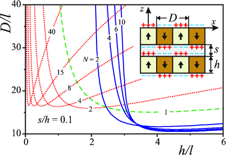
Figure 1: (Color online) Equilibrium period of stripe states in multilayers. For various values of multilayer repeat numbers $N$, the stripe period $D$ in units of the characteristic lengths $l$ is shown for the ferromagnetic mode (dotted line), and antiferromagnetic mode (solid lines) as function of the magnetic layer thickness $h/l$ for the ratio of interlayer to ferromagnetic layer thickness $s/h=0.1$. The dashed line indicates the solutions for a single layer. The inset introduces the geometrical parameters of the model.

Note, that the term “stripe domains” is also commonly used to denote multidomain patterns consisting of stripes with weakly undulating magnetization which, however, stays predominantly in the layer plane Hubert98 . On the other hand, the term band domains is used to describe structures of homogeneous domains with perpendicular magnetization that alternates between up and down direction. These two types of stripe domains should not be confused. In the model for an extended multilayer film, the multilayer is taken to be infinite in $x-$ and $y-$ directions. The stripes with alternating magnetization $\mathbf{M}$ along the $z$ direction and with $|\mathbf{M}|=M\equiv$ const have the period length $D$ and are separated by domain walls of vanishingly small thickness (Fig. 1). However, domain walls contribute a positive excess energy with an area density $\sigma$, which is included in the model as one of the materials parameters. The ferromagnetic layers are antiferromagnetically coupled via a non-ferromagnetic spacer. This interaction imposes antiparallel orientation of the magnetic moments in adjacent layers, while magnetostatic forces favor parallel orientation of the magnetization. As a results of this competition three different ground states can be realized depending on the materials and geometrical parameters of the multilayer stripes . Namely, the homogeneous antiferromagnetic state, and stripe domains with parallel or antiparallel arrangement of the magnetization in adjacent layers (Fig. 2).

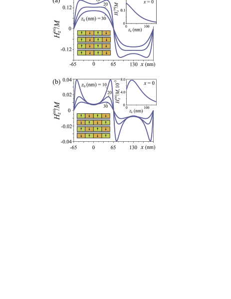
Figure 2: (Color online) Calculated stray-field profiles $H_{z}^{(m)}(x)$ for ferromagnetic (a) and antiferromagnetic (b) modes for [[Co/Pt]₇CoRu]₄ multilayers investigated in Hellwig03 . Insets show the perpendicular stray-field component $H_{z}^{(m)}(z_{0})$ at the center of the stripes in dependency on the distance $z_{0}$ above the multilayer surface. In ferro stripes this function monotonically decreases with increasing $z$, while in antiferro stripes it has a maximum at a finite distance from the surface.

We denote these latter two multidomain modes as ferro and antiferro stripes. The energy density for both types of stripe phases can be written as

$$w_{N}(D)=\frac{2\sigma}{D}\pm\frac{J}{h}\left(1-\frac{1}{N}\right)+2\pi M^{2}\,w_{m}(D)\,.$$ (1)

The first term in $w_{N}$ is the domain wall energy, $J>0$ is the antiferromagnetic exchange interaction via the spacer layer. The stray field energy $w_{m}$ can be expressed as a set of finite integrals FTT80 ; stripes ,

$$w_{m}(D)=1+\Omega(D,h)\mp\frac{1}{N}\sum_{k=1}^{N-1}(N-k)\,\Xi_{k}(D,h,s),$$ (2)

where $T=h+s$ is the period length of the superlattice, $\Xi_{k}=2\,\Omega(D,Tk)\,-\,\Omega(D,Tk+h)\,-\,\Omega(D,Tk-h)$, and

$$\Omega(D,\omega)=\frac{8\,\omega^{2}}{\pi hD}\int_{0}^{1}(1-t)\ln\left|\tanh\left(\frac{\pi\omega t}{D}\right)\right|dt\,.$$ (3)

The upper (lower) sign in Eqs. (1), and in (2) for $w_{m}$, corresponds to ferro(antiferro) stripes. The equilibrium domain configuration of the stripes is derived by minimization of $w_{N}$ with respect to the stripe period $D$ stripes . Introducing a new length scale, based on the characteristic length $l=\sigma/(4\pi M^{2})$, one can express the solutions for reduced periods $D/l$ as functions of three parameters, the reduced geometrical sizes ($h/l$), ($s/l$), and the repeat number of the multilayer $N$. Typical solutions $D/l$ as functions of $h/l$ are presented in Fig. 1. The solutions for ferro stripes exist for arbitrary values of $h$ and $s$. In the two limiting cases of large and small spacer thickness, the solutions asymptotically approach the behavior of the known solutions for individual layers (see Ref. Malek ; Suna85 ) with a thickness $h$ for the case $s\gg h$ and with effective thickness $hN$ for $s\ll h$. The solutions for antiferro stripes with even $N$ exist only in an interval bounded from below, $h>h_{cr}(N)$. The period $D$ tends to infinity at a critical thickness $h_{cr}$. Strictly speaking, for odd $N$ antiferro stripes (similarly to ferro stripes) exist for arbitrarily small layer thickness $h$. However, their periods increases so steeply that a single domain state is practically reached when the period exceeds the lateral size of the layer. The calculated periods for odd-numbered multilayers has similar have similar size as those for antiferro stripes with even $N$. The phase diagrams considering these stripe ground-states show that both types of stripes can exist as stable or metastable states in extended and overlapping ranges of the material parameters stripes . The extended co-existence regions of different types of multidomain states in the phase diagrams also entails the possibility to create complex “interspersed” patterns that consist of subdomains with ferro and antiferro stripes. For identical values of the materials parameters the equilibrium domain widths for ferro and antiferro stripes can differ considerably (see Fig. 1). Hence, the mixed stripe patterns can include regions with different domain sizes. Exactly such structures have been observed in some [Co/Pt]Ru multilayers HellwigPrivate . In addition to the differing characteristic periods of ferro and antiferro stripes, these stripe patterns also cause different distributions of the stray fields $\mathbf{H}^{(m)}$ at the sample surfaces. The stray-fields can be probed by magnetic force microscopy, however, the properties of the stray fields peculiar to the different stripe patterns are rather subtle. Thus, the experimental observation and quantitative evaluation of these differences must be based on a detailed comparison with theoretical model calculations.

Convenient analytical expressions for stray field components and their spatial derivatives for multilayers with ferro and antiferro stripes can be derived from Eqs. (1)–(2). The mathematical equivalence between electro- and magnetostatic problems allows to treat a magnetized layer as a system of “charges” distributed over its surfaces Hubert98 . The stray field above the sample surface can be expressed as a superposition of the stray fields from the 2$N$ interface planes with “charged” stripes (Inset in Fig. 1). By solving the magnetostatic problem for a plane with “charged” stripes (see Appendix) one can write the following solutions for the stray field components $\mathbf{h}^{(m)}(x,z)$

$$h_{x}^{(m)}(x,z)=2M\ln\left|\frac{\cosh\left(2\pi z/D\right)-\sin\left(2\pi x/D\right)}{\cosh\left(2\pi z/D\right)+\sin\left(2\pi x/D\right)}\right|,$$ (4)

$$h_{z}^{(m)}(x,z)=4M\underbrace{\arctan\left[\cos\left(2\pi x/D\right)/\sinh\left(2\pi z/D\right)\right]}_{\upsilon_{0}(x,z)}.$$ (5)

Then the total stray field of the multilayer at a distance $z_{0}$ above the surface can be written as

$$\mathbf{H}^{(m)}(x,z_{0})=\sum_{k=0}^{N-1}\Gamma_{k}\left[\mathbf{h}^{(m)}(x,z_{0}+Tk)\right.$$

$$\left.-\mathbf{h}^{(m)}(x,z_{0}+Tk+h)\right]\,.$$ (6)

The factor $\Gamma_{k}=(-1)^{k}$ holds for antiferro stripes, and $\Gamma_{k}=1$ for ferro stripes. Spatial derivatives of $H_{z}^{(m)}$ with respect to $z$ are important for the analysis of the MFM images. The derivative $\Upsilon_{n}(x,z_{0})=\partial^{n}H_{z}^{(m)}/{\partial z^{n}}$can be derived analytically by differentiation of Eq. (6) as

$$\Upsilon_{n}(x,z_{0})=4M\left(\frac{2\pi}{D}\right)^{n}\ \ \ \ \ \ \ \ \ \ \ \ \ \$$

$$\times\sum_{k=0}^{N-1}\Gamma_{k}\left[\upsilon_{n}(x,z_{0}+Tk)-\upsilon_{n}(x,z_{0}+Tk+h)\right]\,.$$ (7)

We introduce here a set of functions $\upsilon_{n}(x,z)$ which are derivatives of the function $\upsilon_{0}(x,z)$ defined in Eq. (5) with respect to the normalized geometry parameter $\xi=2\pi z/D$,

$$\upsilon_{n}(x,z)\equiv\partial^{n}\upsilon_{0}/\partial\xi^{n}=\cos\left(2\pi x/D\right)\frac{G_{n}(x,z)}{g_{+}^{n}(x,z)},$$ (8)

where

$$g_{\pm}=\left[\cosh\left(4\pi z/D\right)\pm\cos\left(4\pi x/D\right)\right]/2,$$

$$G_{1}=-\cosh\left(2\pi z/D\right),\quad$$

$$G_{2}=\sinh\left(2\pi z/D\right)(1+g_{-}),\;$$

$$G_{3}=-\cosh\left(2\pi z/D\right)(2g_{-}^{2}-g_{+}^{2}+2g_{+}-2),$$

$$G_{4}=\sinh\left(2\pi z/D\right)$$

$$\ \ \ \ \ \ \ \>\times\left[6(g_{-}+1)^{2}(g_{-}-1)+g_{+}^{2}(1-5g_{-})\right]\,.$$

(9)

Together with the equation $dw_{N}/dD=0$, which determines the equilibrium domain period, Eqs. (6) and (7) describe the stray field and its spatial derivatives as a function of the coordinates $x$, $z$ for a multilayer in a stripe state. The stray field $\mathbf{H}^{(m)}(x,z_{0})$ (6) and the derivatives $\Upsilon_{n}(x,z_{0})$ (7) are expressed as sets of analytical functions (4), (5) (8), and (9). The expressions depend on the geometrical parameters and, via the equilibrium domain widths $D$, on the material parameters of the multilayer. These analytical expressions can be readily evaluated by elementary mathematical means.

In order to demonstrate the main features of the stray fields $H_{z}^{(m)}(x,z)$ from the ferro and antiferro stripes we evaluate these functions for a multilayer [[Co/Pt]₇CoRu)]₄ with magnetic and geometrical parameters corresponding to a sample that was investigated experimentally in Hellwig03 . In this superlattice the ferromagnetic constituents are magnetic [Co/Pt]₇ multilayers with thicknesses of the ferromagnetic Co-layers 0.4 nm and thickness of the Pt layer 0.7 nm. The non-ferromagnetic Ru spacer has a thickness of 0.9 nm and mediates an indirect antiferromagnetic interlayer exchange. The domain period has been determined as $D$ = 260 nm Hellwig03 . For ferro and antiferro stripe modes the functions $H_{z}^{(m)}(x,z)$ are markedly different both in the intensity and in the location of characteristic extremal points (Fig. 2 ). Moreover they display qualitatively different functional dependencies on the distance from the multilayer surface $z_{0}$ (see Insets in Fig.2).

The stray-field distribution over the multilayer surface can be viewed as a superposition of magnetostatic fields from systems of “charged” bands. This allows to give a simple physical interpretation for the main features of the stray field profiles in Fig.  2. First we consider ferro stripes. It is convenient to separate the total stray-field over a domain to two contributions: one created by the top and bottom bands of the domain(”self” field), and that produced by all other ”charged” bands. In the domain centers near the sample surface, $z_{0}\ll D$, the stray “self” field is small due to screening effects of the domain top and bottom surfaces. Because the bands change their “charges” at the domain walls the stray field is substantially enhanced above the walls. As a result, the profiles $H_{z}^{(m)}(x,z)$ have characteristic wells in the domain centers for $z_{0}\ll D$. For increasing distance $z_{0}$ from the surface the difference between values of $H_{z}^{(m)}$ in the center and at the domain edges decreases due to the increasing influence of neighbouring poles. For large distances $z_{0}$ the wells disappear and the profiles obtain a typical bell-like shape (compare the traces for $z_{0}$ = 10 and 30 nm in Fig. 2 (a)). The antiferro stripe mode can be obtained from those for ferro stripes by changing the magnetostatic “charges” for the bands in all even layers. This weakens the total stray field and sharpens the difference between the stray fields at the center and near the domain edges. Finally, the competing character of the stray field contributions from odd and even layers causes the nonmonotonic dependence of $H_{z}^{(m)}(z)$ (Inset in Fig.  2 (b)).

Generally the functions $\mathbf{H}^{(m)}(x,z_{0})$, $\Upsilon_{n}^{(F)}(x,z_{0})$, $\Upsilon_{n}^{(AF)}(x,z_{0})$ have a number of characteristic features that can be utilized in new methods to investigate the multidomain modes. One method can be based on measuring the MFM contrast in the center of the domains. In this case $x=kD,\,\,k=0,1,2,3...$ and the functions $\tilde{\upsilon}(z)\equiv\upsilon_{n}(kD,z)$ are reduced to the following expressions

$$\tilde{\upsilon}_{0}(z)=\arccos\left[\tanh\left(2\pi z/D\right)\right],\quad$$

$$\tilde{\upsilon}_{1}(z)=-\cosh^{-1}\left(2\pi z/D\right),$$

$$\tilde{\upsilon}_{2}(z)=\sinh\left(2\pi z/D\right)\cosh^{-2}\left(2\pi z/D\right),\quad$$

$$\tilde{\upsilon}_{3}(z)=-(1-\sinh^{2}\left(2\pi z/D\right))\cosh^{-3}\left(2\pi z/D\right),$$

$$\tilde{\upsilon}_{4}(z)=\sinh\left(2\pi z/D\right)\frac{\sinh^{2}\left(2\pi z/D\right)-5}{\cosh^{4}\left(2\pi z/D\right)}.$$ (10)

Profiles $\tilde{\upsilon}_{n}(z_{0})$ from Eqs. (10) for $n$ = 1,2,3,4 are plotted in Fig. 3. Their characteristic features can be used to ascertain the type of the stripe mode and should even allow quantitative evaluation of magnetic properties in multilayers, if and when they are accessible in experiment.

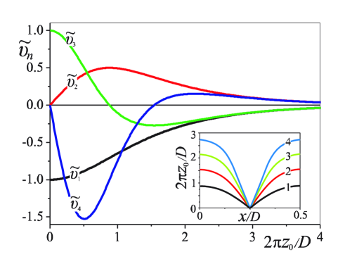
Figure 3: (Color online) Characteristic functions $\tilde{\upsilon}_{n}(z_{0})\equiv\upsilon_{n}(0,z_{0})$ (Eq. (10)) describe MFM images in the center of domains. Inset indicates the location of the extrema of the functions $\upsilon_{n}(x,z_{0})$ in the $xOz$ plane.

Owing to the properties of the magnetic probe, a signal from a magnetic force microscope generally differs strongly from the $H_{z}(x)$ profile. In order to compare the expected outcome of different domain configurations, the MFM contrast has to be calculated for realistic tip models. The MFM signal for a magnetic cantilever oscillating in z-direction is given by Grutter92 ; Lohau99

$$\Delta\Phi = -\frac{Q}{k}\left(\frac{\partial F_{z}}{\partial z}\right)$$ (11)

$$= -\frac{Q}{k}\mu_{0}\int_{tip}\frac{\partial^{2}\left[\mathbf{M}^{(tip)}(\mathbf{r})\cdot\mathbf{H}^{(m)}(\mathbf{r})\right]}{\partial z^{2}}\;dV\,.$$

Here, $\Delta\Phi$ is the measured phase shift between excitation and oscillation due to the force gradient $\partial F_{z}/\partial z$ that acts on the cantilever in the stray field of the sample $\mathbf{H}^{(m)}(\mathbf{r})$. $Q$ and $k$ are the quality factor of the oscillation and the spring constant, respectively. Assuming a rigid tip magnetized in z-direction, i.e., a tip with a homogeneous magnetization distribution, $\mathbf{M}^{(tip)}\equiv$ const throughout the tip volume, that does not change during the scan across the stray field of the sample, the expression for the force gradient simplifies to

$$\frac{\partial F_{z}}{\partial z}=M_{z}^{(tip)}\int_{tip}\frac{\partial^{2}H_{z}^{(m)}(\mathbf{r})}{\partial z^{2}}\;dV\,.$$ (12)

The volume integration is a crucial step as it modifies the signal compared to the profile estimated by the second stray field derivative.

A realistic tip geometry can be modelled by a truncated triangle placed in the x-z-plane (see inset in Fig. 6). This mimics the two parallel sides of the 4-sided pyramidal geometry of a typical MFM tip. The two-dimensional model simplifies considerably the calculations. The error incurred by this reduced model is minor because of the infinite extension of the domain models in the y-direction.

Figure 4: (Color online) Maze domain pattern in [(Co/Pt)₈)CoRu]₁₈ observed by MFM at room temperature (a) and line scans along the marked line for $z_{0}$ = 10, 20, 30, 40 ,50 and 60 nm.

To demonstrate this approach we analyze the MFM contrast measured across a thick [(Co/Pt)₈)CoRu]₁₈ multilayer prepared at Hitachi GST (for details on these multilayers, see Refs. Hellwig03 ). The MFM pictures show a typical maze pattern of ferro stripes with perpendicular magnetization at room temperature Fig. 4 (a)). For comparison with contrast calculations the MFM signal along the marked line of the image was recorded repeatedly (with the slow scan axis disabled) at lift heights of 10, 20, 30, 40, 50 and 60 nm. Averaged scan lines for each lift height in Fig. 4 (b) display a reduced contrast for increasing scan height.

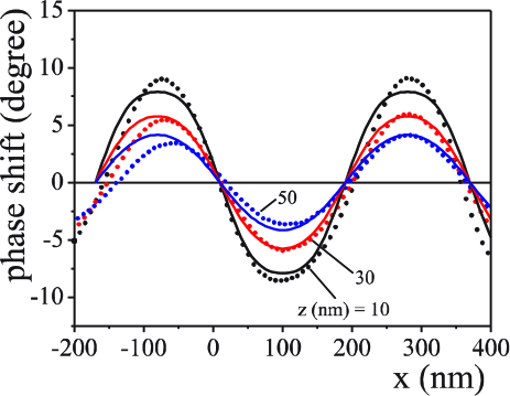
Figure 5: (Color online) Experimental (points) and calculated (solid lines) force gradient profiles [(Co/Pt)₈)CoRu]₁₈ for MFM scans corresponding to the framed area in Fig. 4(b).

The very regular domain pattern in the center of this scan (framed area) was modeled according to Eq. (7) as parallel FM stripes with the period of 360 nm based on an $N=18$ multilayer with the known layer architecture. With the resulting second stray field derivatives the MFM phase shift was computed according to Eq. (7) using the above mentioned tip model. As cantilever parameters a spring constant of $k$ = 2 N/m and a quality factor of $Q$ = 100 were used. The height, pyramid angle and tip apex were chosen as 4 $\mu$m, 30 and 50 nm, respectively, and the film coating was assumed to be 30 nm. As an adjustable parameter the tip magnetization $M_{z}$,tip was set to 3$\cdot$10⁶ A/m. With this reasonable value the computed phase shift magnitude, line profile and lift height dependency compare very well with the experimental data (Fig. 5). Such calculations can thus be used to predict differences in the MFM contrast of the two distinct types of stripe domains.

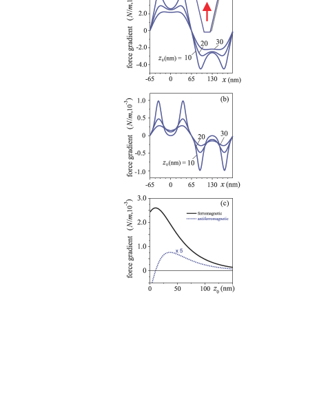
Figure 6: (Color online) Calculated force gradient profiles for a 4-sided pyramidal tip and ferro (a), antiferro (b) modes in the center of domains as function of the distance $z_{0}$ from the surface (c) for [[Co/Pt]₇CoRu]₄ multilayers with the same geometrical parameters as in Fig. 2.

Fig. 6 shows the calculated force gradient profiles for the ferro and antiferro stripes presented in Fig. 2. The profiles reflect general features of the stray-field distributions in the multidomain patterns. Here as well, quantitative and qualitative differences allow to distinguish ferro and antiferro stripes. The signal from the antiferro stripes is clearly weakened, but it is large enough to be measured in a typical MFM setup which allows the detection of a few 10 $\mu$N/m (10^-2 dyn/cm) Schendel00 . However, as quantitative MFM measurements are still rare and require precise calibration routines Schendel00 ; Lohau99 the absolute value of the signal is not a reliable criterion for the distinction between different stripe configurations. More importantly, the force gradient directly above the center of a domain shows a monotonically decreasing signal strength for increasing scan height $z_{0}$ in case of the ferro stripes. Above the antiferro stripes, on the other hand, the force gradient is increasing with increasing scan height, at least in the range from 10 to 30 nm. This qualitative difference is demonstrated again in Fig. 6, where the force gradient experienced by a realistic tip model is plotted as a function of $z_{0}$ for the two cases. The non-monotonic behavior of the force gradients observed above a multidomain structure can be taken as a clear fingerprint of an antiferro stripe state within a multilayer stack. The calculation even reveals a sign change as an additional signature of the antiferro stripes, but this appears at a scan height smaller than 10 nm, which is experimentally very difficult to access, as topographic information can influence the measurement.

The solutions for the stray field (6) and its derivatives (7) can be simplified in the practically important case of large domains, $D\gg h$. Expansion of $\Upsilon_{n}(x,z_{0})$ with respect to the small parameter $h/D\ll 1$ yields for ferro stripes

$$\Upsilon_{n}^{(F)}(x,z)=-4MN\left(2\pi/D\right)^{n}\;\upsilon_{n+1}(x,z),$$ (13)

and for antiferro stripes with even $N$

$$\Upsilon_{n}^{(AF)}(x,z)=-2MN\!\left(2\pi/D\right)^{n}(1\!+\!s/h)\upsilon_{n+2}(x,z).$$ (14)

For antiferro stripes in multilayers with odd $N$ the functions $\Upsilon_{n}(x,z)$ are given by Eq. (13). Note that the functions $\Upsilon_{n}^{(F)}$ from the Eq. (13) are proportional to $\upsilon_{n+1}$, while the functions $\Upsilon_{n}^{(AF)}$ in Eq. (14) can be expressed by derivative of the functions $\upsilon_{n+1}$ through the relation $\upsilon_{n+2}=\partial\upsilon_{n+1}/\partial z$. This means that in this limit of large domains, the functions $\Upsilon_{n}$ in the antiferro mode behave as $z$-derivatives of the corresponding functions of ferro modes. In particular for $n=0$, the Eqs. (13) and (14) give the perpendicular stray field components for ferro stripes and antiferro stripes with odd $N$, correspondingly, by the expressions

$$H_{z}^{(F)}(x,z_{0})=-4MN\;\upsilon_{1}(x,z_{0}),$$

$$H_{z}^{(AF)}(x,z_{0})=-2MN(1+s/h)\;\upsilon_{2}(x,z_{0}).$$ (15)

In conclusion, we have presented analytical solutions for the stray field (Eq. (6)) and its spatial derivatives (Eq. (7)) in multidomain states of magnetic multilayers with out-of-plane magnetization. These solutions can be applied to calculate the MFM contrast for a realistic tip geometry using Eq. (12). It is shown that the ground-state ferro and antiferro stripe structures in antiferromagnetically coupled multilayers differ by their period lengths and by the spatial distribution of their stray-fields. Our analytical calculations executed within a simplified model of one-dimensional multidomain patterns with fixed magnetization orientation and infinitely thin domain walls are able to reproduce the general features of MFM images from antiferromagnetically coupled multilayers. These features can be used to identify different types of multidomain patterns and extract values of the magnetic interactions. They also create a basis for more detailed investigations on more realistic models. Such models should consider distortions of the magnetization with tilting away from the perpendicular direction in sizeable fractions of the domains due to the finite strength of uniaxial anisotropy, or a finite width of the domain walls between domains combined with the appearance of magnetic charge distributions at the walls. Additionally, it was recently shown that ferro stripes are unstable with respect to a lateral shift of domains in adjacent layersAPLshift . This creates specific multidomain patterns with distinct modulations across the multilayer stack. Such effects can be consistently taken into account by numerical solutions of the micromagnetics equations for specific cases. Here, we have analyzed the backbone structure for all of these types of spatially inhomogeneous distributions of the magnetization within the multilayer and stray fields over its surface.

Acknowledgments

The authors thank O. Hellwig, J. McCord, A. T. Onisan, and R. Schäfer for helpful discussions. We also thank O. Hellwig (Hitachi GST) for providing the Co/Pt/Ru multilayer sample and C. Bran for performing the MFM measurements. Work supported by DFG through SPP1239, project A8. N.S.K., I.E.D, and A.N.B. thanks H. Eschrig for support and hospitality at IFW Dresden.

Appendix

The scalar potential of a sheet with “charged” stripes (Inset Fig. 1) can be derived by solving Poisson’s equation (see, e.g., Malek ; Suna85 )

$$\phi(x,z)=\frac{4MD}{\pi}\ \ \ \ \ \ \ \ \ \ \ \ \ \ \ \ \ \$$

$$\times\sum_{n=1}^{\infty}\frac{\sin(\pi n/2)}{n^{2}}\cos\left(2\pi nx/D\right)\exp\left(-2\pi nz/D\right)\,.$$ (16)

Using the identity $n^{-m}=[(m-1)!]^{-1}\int_{0}^{\infty}t^{m-1}e^{-nt}dt$ the Eq. (16) can be transformed into the following form FTT80 ; stripes

$$\phi(x,z)=\frac{8M\!D}{\pi}\!\int\limits_{0}^{\infty}\!\frac{\cos(2\pi x/D)\cosh(t+2\pi z/D)tdt}{\cosh^{2}(t+2\pi z/D)-\sin^{2}(2\pi x/D)}\;.$$

(17)

From this closed expression, the components of the stray field $\mathbf{h}^{(m)}=-\nabla\phi$ are readily derived in the analytical form given by Eqs. (4) and (5).

References

- (1) T. M. Maffitt et al., IBM. J. Res. & Dev. 50, 25 (2006); S.A. Wolf, D. Treger, A. Chtchelkanova, MRS Bull. 31, 400 (2006).
- (2) S. Hamada, K. Himi, T. Okuno, K. Takanashi, J. Magn. Magn. Mater. 240, 539 (2002).
- (3) O. Hellwig, et al. Nature Mater. 2, 112 (2003); O. Hellwig, A. Berger, E. E. Fullerton, Phys. Rev. Lett. 91, 197203 (2003); O. Hellwig, A. Berger, E. E. Fullerton, J. Magn. Magn. Mater. 290-291, 1 (2005).
- (4) H. Itoh, et al. J. Magn. Magn. Mater. 257, 184 (2003); Z.Y. Liu, S. Adenwalla, Phys. Rev. Lett. 91, 037207 (2003).
- (5) A. Baruth et al., Phys. Rev. B 74, 054419 (2006); Appl. Phys. Lett. 89, 202505 (2006).
- (6) U. K. Rößler, A. N. Bogdanov, J. Magn. Magn. Mater. 269, L287 (2004).
- (7) A. N. Bogdanov, U. K. Rößler, cond-mat/0606671 (2006).
- (8) V. Neu, S. Melcher, U. Hannemann, S. Fähler, L. Schultz, Phys. Rev. B 70, 144418 (2004).
- (9) H. J. Hug et al. J. Appl. Phys. 79 5609 (1996); J. Appl. Phys. 83 5609 (1998).
- (10) A. Hubert, R. Schäfer, Magnetic Domains (Springer-Verlag, Berlin, 1998).
- (11) A. N. Bogdanov, D. A. Yablonskii. Fiz. Tverd. Tela 22, 680 (1980), [Sov. Phys. Solid State 22, 399 (1980)].
- (12) Z. Málek, V. Kamberský, Czech. J. Phys. 8, 416 (1958); C.Kooy, U. Enz, Philips Res. Repts. 15, 7 (1960).
- (13) A. Suna, J. Appl. Phys. 59, 313 (1986); H. J. G. Draaisma, W. J. M. de Jonge, J. Appl. Phys. 62, 3318 (1987).
- (14) O. Hellwig, private communication.
- (15) P. Grütter, H. J. Mamin, D. Rugar, in Scanning Tunneling Microscopy II, edited by R. Wiesendanger and H.-J. Güntherodt (Springer, Berlin, 1992), pp. 151-207.
- (16) J. Lohau et al. J. Appl. Phys. 86 3410 (1999).
- (17) P. J. A. van Schendel, H. J. Hug, B. Stiefel, S. Martin, H.-J. Güntherodt, J. Appl. Phys. 88 435 (2000).
- (18) N. S. Kiselev, I. E. Dragunov, U. K. Rößler, A. N. Bogdanov, Appl. Phys. Lett. 91 132507 (2007).