Nonlinear option pricing models for illiquid markets: scaling properties and explicit solutions

Abstract

Several models for the pricing of derivative securities in illiquid markets are discussed. A typical type of nonlinear partial differential equations arising from these investigation is studied. The scaling properties of these equations are discussed. Explicit solutions for one of the models are obtained and studied.

url]http://www2.hh.se/staff/ljbo/

url]www.math.uni-leipzig.de/ frey

AMS subject classification.

35K55, 22E60, 34A05

1 Introduction

Standard derivative pricing theory is based on the assumption of frictionless and perfectly liquid markets. In particular, it is assumed that all investors are small relative to the market so that they can buy arbitrarily large quantities of the underlying assets without affecting its price (perfectly liquid markets). Given the scale of hedging activities on many financial markets this is clearly unrealistic. Hence in recent years a number of approaches for dealing with market illiquidity in the pricing and the hedging of derivative securities have been developed. The financial framework that is being used differs substantially between model classes. However, as shown in Section 2 below, in all models derivative prices can be characterized by fully nonlinear versions of the standard parabolic Black-Scholes PDE. Moreover, these nonlinear Black-Scholes equations have a very similar structure. This makes these nonlinear Black-Scholes equations a useful reference point for studying derivative asset analysis under market illiquidity. In Sections 3 we therefore study scaling properties and compute explicit solutions for a typical fully nonlinear Black-Scholes equation; Section 4 is devoted to studying properties of solutions and sensitivities with respect to model parameters. The relevant literature is discussed in the body of the paper.

2 Illiquid markets and nonlinear Black-Scholes equations

In order to motivate the subsequent analysis we present a brief synopsis of three different frameworks for modeling illiquid markets. We group them under the labels a)transaction-cost models; b) reduced-form SDE-models; c) reaction-function or equilibrium models. In particular, we show that the value function of a certain type of selffinancing strategies (so called Markovian strategies) must be a solution of a fully nonlinear version of the standard Black-Scholes equation. In all models there will be two assets, a risk-free money-market account $B$ which is perfectly liquid and a risky and illiquid asset $S$ (the stock). Without loss of generality, we use the money market account as numeraire; hence $B_{t}\equiv 1$, and interest rates can be taken equal to zero.

(Quadratic) transaction-cost models. The predominant model in this class has been put forward by Cetin, Jarrow and Protter [7]. In this model there is a fundamental stock price process $S^{0}$ following geometric Brownian motion,

$$dS_{t}^{0}=\mu S_{t}^{0}dt+\sigma S_{t}^{0}dW_{t}$$ (2.1)

for constants $\mu\in\mathbb{R}$, $\sigma>0$ and a standard Brownian motion $W$. The transaction price to be paid at time $t$ for trading $\alpha$ shares is

$$\bar{S}_{t}(\alpha)=e^{\rho\alpha}S_{t}^{0},\quad\alpha\in\mathbb{R},\,\,\,\rho>0,$$ (2.2)

where $\rho$ is a liquidity parameter.

Intuitively, in the model (2.2) a trader has to pay a spread whose size relative to the fundamental price, $S_{t}^{0}(e^{\rho\alpha}-1)$, depends on the amount $\alpha$ which is traded. As shown by [7], this leads to transaction costs which are proportional to the quadratic variation of the stock trading strategy. In order to formulate this statement more precisely we consider a selffinancing trading strategy $(\Phi_{t},\eta_{t})_{t\geq 0}$ giving the number of stocks and the position in the money market for predictable stochastic processes $\Phi$ and $\eta$. The value of this strategy at time $t$ equals $V_{t}=\Phi_{t}S_{t}^{0}+\eta_{t}$.

Consider now a Markovian strategy, i.e. a trading strategy of the form $\Phi_{t}=\phi(t,S_{t}^{0})$ for a smooth function $\phi$. In this case $\Phi$ is a semimartingale with quadratic variation given by

$$[\Phi]_{t}=\int_{0}^{t}\left(\phi_{S}(s,S^{0}_{s})\sigma S_{s}^{0}\right)^{2}ds\,;$$

see for instance Chapter 2 of [22]. Then Theorem A3 of [7] yields the following dynamics of $V_{t}$

$$dV_{t}=\phi(t,S_{t}^{0})dS_{t}^{0}-\rho S_{t}^{0}d[\Phi]_{t}=\phi(t,S_{t}^{0})dS_{t}^{0}-\rho S_{t}^{0}\left(\phi_{S}(t,S^{0}_{t})\sigma S_{t}^{0}\right)^{2}dt.$$ (2.3)

Note that according to (2.3), the market impact of the large trader leads to an extra transaction-cost term of size $\rho\int_{0}^{t}S_{s}^{0}\,d[\Phi]_{s}$ in the wealth dynamics.

Suppose now that $u$ and $\phi$ are smooth functions such that $u(t,S_{t}^{0})$ gives the value of a selffinancing trading strategy with stock position $\phi(t,S_{t}^{0})$. According to the Itô formula, the process $(u(t,S_{t}^{0}))_{t\geq 0}$ has dynamics

$$du(t,S_{t}^{0})=u_{S}(t,S_{t}^{0})dS_{t}^{0}+\left(u_{t}(t,S_{t}^{0})+\frac{1}{2}\sigma^{2}(S_{t}^{0})^{2}u_{SS}(t,S_{t}^{0})\right)\,dt\,.$$

Comparing this with (2.3), using the uniqueness of semimartingale decompositions it is immediate that $u$ must satisfy the PDE $u_{t}+\frac{1}{2}\sigma^{2}S^{2}u_{SS}+\rho S^{3}\sigma^{2}\phi_{S}=0$ and that moreover $\phi=u_{S}$. The last relation gives $\phi_{S}=u_{SS}$, so that we obtain the following nonlinear PDE for $u$

$$u_{t}+\frac{1}{2}\sigma^{2}S^{2}u_{SS}\left(1+2\rho Su_{SS}\right)=0\,.$$ (2.4)

When pricing a derivative security with maturity date $T$ and payoff $h(S_{T})$ for some function $h:[0,\infty)\to\mathbb{R}$ we have to add the terminal condition $u(T,S)=h(S)$, $S\geq 0$. For instance, in case of a European call option with strike price $K>0$ we have $h(S)=\max\{S-K,0\}$.

Note that the original paper [7] goes further in the analysis of quadratic transaction cost models. To begin with, a general framework is proposed that contains (2.2) as special (but typical) case. Moreover, conditions for absence of arbitrage for a general class of trading strategies - containing Markovian trading strategies as special case - are given, and a notion of approximative market completeness is studied.

Reduced-form SDE models. Under this modeling approach it is assumed that investors are large traders in the sense that their trading activity affects equilibrium stock prices. More precisely, given a liquidity parameter $\rho\geq 0$ and a semimartingale $\Phi$ representing the stock trading strategy of a given trader, it is assumed that the stock price satisfies the SDE

$$dS_{t}=\sigma S_{t}dW_{t}+\rho S_{t}d\Phi_{t}\,.$$ (2.5)

The intuitive interpretation is as follows given that the investor buys (sells) stock ($\Delta\Phi_{t}>0$) the stock price is pushed (downward) upward by $\rho S_{t-}\Delta\Phi_{t}$; the strength of this price impact depends on the parameter $\rho$. Note that for $\rho=0$ the asset price simply follows a Black-Scholes model with reference volatility $\sigma$. The model (2.5) is studied among others in [10], [11], [14] or [18].

In the sequel we denote the asset price process which results if a large uses a particular trading strategy $\Phi$ by $S^{\Phi}$. Suppose as before that the trading strategy is Markovian, i.e. of the form $\Phi_{t}=\phi(t,S_{t})$ for a smooth function $\phi$. Applying the Itô formula to (2.5) shows that $S^{\phi}$ is an Itô process with dynamics

$$dS_{t}^{\phi}=v^{\phi}(t,S_{t}^{\phi})S_{t}^{\phi}dW_{t}+b^{\phi}(t,S_{t}^{\phi})S_{t}^{\phi}dt$$

with adjusted volatility given by

$$v^{\phi}(t,S)=\frac{\sigma}{1-\rho S\phi_{S}(t,S)}\,;$$ (2.6)

see for instance [10] for details. In the model (2.5), a portfolio with stock trading strategy $\Phi$ and value $V$ is termed selffinancing, if satisfies the equation $dV_{t}=\Phi_{t}dS_{t}^{\Phi}$. Note that the form of the strategy $\Phi$ affects the dynamics of $S$; this feedback effect will give rise to nonlinearities in the wealth dynamics as we now show. Suppose that $V_{t}=u(t,S_{t})$ and $\Phi_{t}=\phi(t,S_{t})$ for smooth functions $u$ and $\phi$. As before, applying the Itô formula to the process $(u(t,S_{t}^{\phi}))_{t\geq 0}$ yields $\phi_{t}=u_{S}$. Moreover, $u$ must satisfy the relation $u_{t}+\frac{1}{2}(v^{\phi})^{2}(t,S)S^{2}u_{SS}=0$. Using (2.6) and the relation $\phi_{S}=u_{SS}$ we thus obtain the following fully nonlinear PDE for $u(t,S)$

$$u_{t}+\frac{1}{2}\frac{\sigma^{2}}{(1-\rho Su_{SS})^{2}}S^{2}u_{SS}=0\,.$$ (2.7)

Again, for pricing derivative securities a terminal condition corresponding to the particular payoff at hand needs to be added.

Equilibrium or reaction-function models. Here the model primitive is a smooth reaction function $\psi$ that gives the equilibrium stock price $S_{t}$ at time $t$ as function of some fundamental value $F_{t}$ and the stock position of a large trader. A reaction function can be seen as reduced-form representation of an economic equilibrium model, such as the models proposed in [12], [21] or [23]. In these models there are two types of traders in the market: ordinary investors and a large investor. The overall supply of the stock is normalized to one. The normalized stock demand of the ordinary investors at time $t$ is modelled as a function $D(F_{t},x)$ where $x$ is the proposed price of the stock. The normalized stock demand of the large investor is written the form $\rho\Phi_{t}$; $\rho\geq 0$ is a parameter that measures the size of the trader’s position relative to the total supply of the stock. The equilibrium price $S_{t}$ is then determined by the market clearing condition

$$D(F_{t},S_{t})+\rho\Phi_{t}=1\,.$$ (2.8)

Under suitable assumptions on $D$ equation (2.8) admits a unique solution, hence $S_{t}$ can be expressed as a function $\psi$ of $F_{t}$ and $\rho\Phi_{t}$, i.e. $S_{t}=\psi(F_{t},\rho\Phi_{t})$. For instance we have in [21] $\psi(f,\alpha)=f\exp(\alpha)$; the model used in [12] and [25] leads to the reaction function $\psi(f,\alpha)=f/(1-\alpha)\,.$ The reaction-function approach is also used in [15] and in [9].

Now we turn to the characterization of selffinancing hedging strategies in reaction-function models. Throughout we assume that the fundamental-value process $F$ follows a geometric Brownian motion with volatility $\sigma$ (see (2.1)). Moreover, we assume that the reaction function is of the form $\psi(f,\alpha)=fg(\alpha)$ for some increasing function $g$. This holds for the specific examples introduced above and, more generally, for any model where $D(f,x)=U(f/x)$ for a strictly increasing function $U\colon(0,\infty)\to\mathbb{R}$ with suitable range.

Assuming as before that the normalized trading strategy of the large trader is of the form $\rho\phi(t,S)$ for a smooth function $\phi$ we get from Itô’s formula, since $S_{t}=g(\rho\phi(t,S_{t}))F_{t}$,

$$dS_{t}=g(\rho\phi(t,S_{t}))\,dF_{t}+\rho F_{t}g_{\alpha}(\rho\phi(t,S_{t}))\phi_{S}(t,S_{t})\,dS_{t}+b(t,S_{t})\,dt;$$

the precise form of $b(t,S_{t})$ is irrelevant for our purposes. Rearranging and integrating the expression $\big{(}1-\rho F_{t}g_{\alpha}(\rho\phi(t,S_{t}))\phi_{S}(t,S_{t})\big{)}^{-1}$ over both sides of this equation gives the following dynamics of $S$:

$$dS_{t}=\frac{1}{1-\rho\frac{g_{\alpha}(\rho\phi(t,S_{t}))}{g(\rho\phi(t,S_{t}))}S_{t}\phi_{S}(t,S_{t})}\sigma S_{t}dW_{t}+\tilde{b}(t,S_{t})dt\,.$$ (2.9)

Remark 2.1

A very general analysis of the dynamics of selffinancing strategies in reaction-function models (and generalizations thereof) using the Itô-Wentzell formula can be found in [1].

A similar reasoning as in the case of the reduced-form SDE models now gives the following PDE for the value function $u(t,S)$ of a selffinancing strategy

$$u_{t}+\frac{1}{2}\frac{\sigma^{2}}{\left(1-\rho\frac{g_{\alpha}(\rho u_{S})}{g(\rho u_{S})}Su_{SS}\right)^{2}}S^{2}u_{SS}=0\,.$$ (2.10)

In particular, for $g(\alpha)=\exp(\alpha)$ we have $g=g_{\alpha}$ and (2.10) reduces to equation (2.7); for $g(\alpha)={1}\big{/}{(1-\alpha)}$ as in [12], [25], we get the PDE

$$u_{t}+\frac{1}{2}\frac{\sigma^{2}(1-\rho u_{S})^{2}}{\left(1-\rho u_{S}-\rho Su_{SS}\right)^{2}}S^{2}u_{SS}=0\,.$$ (2.11)

Nonlinear Black-Scholes equations. The nonlinear PDEs (2.4), (2.7) , (2.10) and (2.11) are all of the form

$$u_{t}+\frac{1}{2}\sigma^{2}v(S,\rho u_{S},\rho u_{SS})S^{2}u_{SS}=0\,,$$ (2.12)

where $v(S,0,0)=1$. Since $\rho$ is often considered to be small, it is of interest to replace $v$ with its first order Taylor approximation around $\rho=0$. It is immediately seen that for the equations (2.7) and (2.11) this linearization is given by ${v}(S,\rho u_{S},\rho u_{u_{S}S})\approx 1+\rho Su_{SS};$ replacing $v$ with this first order Taylor approximation in (2.7) and (2.11) thus immediately leads to the PDE (2.4).

Note that (2.12) is a fully nonlinear equation in the sense that the coefficient of the highest derivative is a nonlinear function of this derivative. A similar feature can be observed for the limiting price in certain transaction cost models under a proper rescaling of transaction cost and trading frequency; see for instance [2]. Nonlinear PDEs for incomplete markets obtained via exponential utility indifference hedging such as [3] or [19] on the other hand are quasi-linear equations in the sense that the highest derivative $u_{SS}$ enters the equation in a linear way, similar to the well-known reaction-diffusion equations arising in physics or chemistry. From an analytical point of view the nonlinearities arising in both cases are quite different. In the latter quasi-linear case we have to do with a regular perturbation of the classical Black-Scholes (BS) equation but in the case (2.10) we have to do with singular perturbation, meaning that the highest derivative is included in the perturbation [16]. In case of a regular perturbation it is typical to look for a representation of a solutions to a quasi-linear equation in the form

$$u\left(S,t\right)=u_{BS}(S,t)+\sum_{n=1}^{N}\rho u_{1}(S,t)+O(\rho^{N+1}).$$ (2.13)

For many forms of nonlinearities the uniform convergence as $\rho\to 0$ of the expansions of type (2.13) can be established. If the perturbation is of the singular type, the asymptotic expansion of type (2.13) typically breaks down for some $S,t$ and some $N\geq 0$. It can as well happens that the definition domain for the solutions of type (2.13) include just one point or that it is empty. It is very important to obtain explicit solutions for such models because in these case we can not hope to get good approximations for solutions by expansions of the type (2.13) in the whole region.

3 Invariant Solutions for a Nonlinear Black-Scholes Equation

Our goal in this section is to investigate the nonlinear Black-Scholes equation (2.7) using analytical methods. As we have just seen, this equation is typical for the nonlinearities arising in pricing equations for derivatives in illiquid markets in general. Using the symmetry group and its invariants the partial differential equation (2.7) can be reduced in special cases to ordinary differential equations. In [6] a special family of invariant solutions to the equation (2.7) was studied; in particular, the explicit solutions were used as test case for various numerical methods. In the present paper we study all invariant solutions to equation (2.7).

3.1 General Results

In order to describe the symmetry group of (2.7) we use results from Bordag  [5]. In that paper the slightly more general equation

$$u_{t}+\frac{\sigma^{2}S^{2}}{2}\frac{u_{SS}}{(1-\rho\lambda(S)Su_{SS})^{2}}=0,$$ (3.14)

with a continuous function $\lambda:(0,\infty)\to(0,\infty)$ is studied (note that for $\lambda\equiv 1$ this equation reduces to (2.7)) and the following theorem was proved.

Theorem 3.1

The action of the symmetry group $G_{\Delta}$ of (3.14) with an arbitrary function $\lambda(S)$ is given by

$${\tilde{S}} = S,$$ (3.15)

$${\tilde{t}} = t+a_{2}\epsilon,$$ (3.16)

$${\tilde{u}} = u+a_{3}S\epsilon+a_{4}\epsilon,~{}~{}\epsilon\in(-\infty,\infty).$$ (3.17)

If the function $\lambda(S)$ has the special form $\lambda(S)=\omega S^{k},~{}k,\omega\in{\mathbb{R}}$, equation (3.14) takes the special form

$$u_{t}+\frac{\sigma^{2}S^{2}}{2}\frac{u_{SS}}{(1-bS^{k+1}u_{SS})^{2}}=0\,,b=\omega\rho.$$ (3.18)

In that case the symmetry group $G_{\Delta}$ has the richer structure

$${\tilde{S}} = Se^{a_{1}\epsilon},~{}~{}\epsilon\in(-\infty,\infty),$$ (3.19)

$${\tilde{t}} = t+a_{2}\epsilon,$$

$${\tilde{u}} = ue^{a_{1}(1-k)\epsilon}+\frac{a_{3}}{a_{1}k}S\epsilon e^{a_{1}\epsilon}(1-e^{-a_{1}k\epsilon})$$ (3.20)

$$+ \frac{a_{4}}{a_{1}(1-k)}(e^{a_{1}(1-k)\epsilon}-1),~{}~{}k\neq 0,~{}k\neq 1$$

$${\tilde{u}} = ue^{a_{1}\epsilon}+a_{3}S\epsilon e^{a_{1}\epsilon}+\frac{a_{4}}{a_{1}}(e^{a_{1}\epsilon}-1),~{}k=0,$$

$${\tilde{u}} = u+\frac{a_{3}}{a_{1}}S(e^{a_{1}\epsilon}-1)+a_{4}\epsilon,~{}k=1.$$ (3.21)

The proof is based on methods of Lie point symmetries, i.e. the Lie symmetry algebras and groups to the corresponding equations were found; see [5] for details and [17, 20, 13] for a general introduction to the methodology. As we will see later, the solutions found in [5] for the case $\lambda(S)=S$ can be used to obtain the complete set of invariant solutions to equation (2.7).

For $\lambda(S)=\omega S^{k}$ with $k=0,1$ we can use (3.19) to obtain a new independent invariant variable $z$ and (3.21) to obtain a new dependent variable $v$; these variables are given by

$$z = \log S+at,~{}~{}a\neq 0,$$

$$v = u~{}S^{(k-1)},~{}~{}k=0,1.$$ (3.22)

Using these variables we can reduce the partial differential equation (3.18) to the ordinary differential equation

$$v_{z}+q\frac{v_{zz}+\xi v_{z}}{(1-b(v_{zz}+\xi v_{z}))^{2}}=0,\,$$ (3.23)

where $q=\frac{\sigma^{2}}{2a},~{}a\neq 0,b=\omega\rho\neq 0,\xi=(-1)^{k},~{}k=0,1.$ It is a straightforward consequence of Theorem 3.1 that these are the only nontrivial invariant variables. In the sequel we will determine explicit solutions for (3.23) for the case $k=0$ which corresponds to the original equation (2.7).

Remark 3.1

Equation (3.23) with $k=0$ and $k=1$ are related to each other. Note however, that the relation between the corresponding solutions is not so straightforward, because (3.23) is nonlinear and we need real valued solutions. Hence the results from [5] - where (3.23) was studied for the case $k=1$ - do not carry over directly to the present case $k=0$, so that a detailed analysis of the case $k=0$ is necessary.

To find families of invariant solution we introduce a new dependent variable

$$y(z)=v_{z}(z).$$ (3.24)

If we assume that the denominator of the equation (3.23) is different from zero, we can multiply both terms of equation (3.23) by the denominator of the second term and obtain

$$yy_{z}^{2}+2\xi\left(y^{2}-\xi\frac{1}{b}y+\xi\frac{q}{2b^{2}}\right)y_{z}+\left(y^{2}-\xi\frac{2}{b}y+\left(\frac{1+\xi q}{b^{2}}\right)\right)y=0,~{}~{}b\neq 0.$$ (3.25)

We denote the left hand side of this equation by $F(y,y_{z})$. The equation (3.25) can possess exceptional solutions which are the solutions of a system

$$\frac{\partial F(y,y_{z})}{\partial y_{z}}=0,~{}~{}F(y,y_{z})=0.$$ (3.26)

The first equation in this system defines a discriminant curve which has the form

$$y(z)=\frac{q}{4b}.$$ (3.27)

If this curve is also a solution of the original equation (3.25) then we obtain an exceptional solution to equation (3.25). We obtain an exceptional solution if $q=-4\xi$, i.e. $a=\xi\sigma^{2}/8$. It has the form

$$y(z)=-\frac{\xi}{b},~{}~{}\xi=(-1)^{k},k=0,1.$$ (3.28)

This solution belongs to the family of solutions (3.30) by the specified value of the parameter $q$. In all other cases the equation (3.25) does not possess any exceptional solutions.

Hence the set of solutions of equation (3.25) is the union of the solution sets of following equations

$$y = 0,$$ (3.29)

$$y = \left(\xi\pm\sqrt{q}\right)/b,$$ (3.30)

$$y_{z} = \left(-\xi y^{2}+\frac{1}{b}y-\frac{q}{2b^{2}}-\sqrt{\frac{q}{b^{3}}\left(\frac{q}{4b}-y\right)}\right)\frac{1}{y},~{}y\neq 0$$ (3.31)

$$y_{z} = \left(-\xi y^{2}+\frac{1}{b}y-\frac{q}{2b^{2}}+\sqrt{\frac{q}{b^{3}}\left(\frac{q}{4b}-y\right)}\right)\frac{1}{y},~{}y\neq 0$$ (3.32)

where one of the solutions (3.30) is an exceptional solution (3.28) by $q=-4\xi$ for $k=1$. In case $k=0$ we have $\xi=1$ so that solutions of (3.30) are complex valued functions. We denote the right hand side of equations (3.31), (3.32) by $f(y)$. The Lipschitz condition for equations of the type $y_{z}=f(y)$ is satisfied in all points where the derivative $\frac{\partial f}{\partial y}$ exists and is bounded. It is easy to see that this condition will not be satisfied by

$$y=0,~{}~{}y=\frac{q}{4b},~{}~{}y=\infty.$$ (3.33)

Hence on the lines (3.33) the uniqueness of solutions of equations (3.31), (3.32) can be lost. We will study in detail the behavior of solutions in the neighborhood of the lines (3.33). For this purpose we look at the equation (3.25) from another point of view. If we assume now that $z,y,y_{z}$ are complex variables and denote

$$y(z)=\zeta,~{}~{}y_{z}(z)=w,~{}~{}\zeta,w\in C,$$ (3.34)

then the equation (3.25) takes the form

$$F(\zeta,w)=\zeta w^{2}+2\xi\left(\zeta^{2}-\xi\frac{1}{b}\zeta+\xi\frac{q}{2b^{2}}\right)w+\left(\zeta^{2}-\xi\frac{2}{b}\zeta+\frac{1+\xi q}{b^{2}}\right)\zeta=0,$$ (3.35)

where $b\neq 0.$ The equation (3.35) is an algebraic relation in $C^{2}$ and defines a plane curve in this space. The polynomial $F(\zeta,w)$ is an irreducible polynomial if at all roots $w_{r}(z)$ of $F(\zeta,w_{r})$ either the partial derivative $F_{\zeta}(\zeta,w_{r})$ or $F_{w}(\zeta,w_{r})$ are non equal to zero. It is easy to prove that the polynomial (3.35) is irreducible.

We can treat equation (3.35) as an algebraic relation which defines a Riemannian surface $\Gamma~{}:~{}F(\zeta,w)=0~{}$ of $w=w(\zeta)$ as a compact manifold over the $\zeta$-sphere. The function $w(\zeta)$ is uniquely analytically extended over the Riemann surface $\Gamma$ of two sheets over the $\zeta-$sphere. We find all singular or branch points of $w(\zeta)$ if we study the roots of the first coefficient of the polynomial $F(\zeta,w)$, the common roots of equations

$$F(\zeta,w)=0,~{}~{}F_{w}(\zeta,w)=0,~{}~{}~{}\zeta,w\in C\cup{\infty}.$$ (3.36)

and the point $\zeta=\infty.$ The set of singular or branch points consists of the points

$$\zeta_{1}=0,~{}~{}\zeta_{2}=\frac{q}{4b},~{}~{}\zeta_{3}={\infty}.$$ (3.37)

As expected we got the same set of points as in real case (3.33) by the study of the Lipschitz condition but now the behavior of solutions at the points is more visible.

The points $\zeta_{2},\zeta_{3}$ are the branch points at which two sheets of $\Gamma$ are glued on. We remark that

$$w(\zeta_{2})=-\frac{1}{b}\left(1-\xi\frac{q}{4}\right)-t\frac{4\xi}{\sqrt{-bq}}+\cdots,~{}~{}t^{2}=\zeta-\frac{q}{4b},$$ (3.38)

where $t$ is a local parameter in the neighborhood of $\zeta_{2}.$ For the special value of $q=4\xi$, i.e. k=0, the value $w(\zeta_{2})$ is equal to zero.

At the point $\zeta_{3}=\infty$ we have

$$w(\zeta)=-\frac{\xi}{t^{2}}+\frac{1}{b}-\xi t\sqrt{\frac{-q}{4b^{3}}},~{}~{}t^{2}=\frac{1}{\zeta},~{}~{}\zeta\to\infty,$$

where $t$ is a local parameter in the neighborhood of $\zeta_{3}.$ At the point $\zeta_{1}=0$ the function $w(\zeta)$ has the following behavior

$$w(\zeta) \sim -\frac{q}{b^{2}}\frac{1}{\zeta},~{}\zeta\to\zeta_{1}=0,~{}{\mbox{on the principal sheet}},$$ (3.39)

$$w(\zeta) \sim -\left(\xi+\frac{1}{q}\right)\zeta,~{}\zeta\to\zeta_{1}=0,~{}q\neq 1,~{}~{}{\mbox{on the second sheet}},$$ (3.40)

$$w(\zeta) \sim -2b^{2}\zeta^{2},~{}\zeta\to\zeta_{1}=0,~{}q=1,~{}~{}{\mbox{on the second sheet}}.$$ (3.41)

Any solution $w(\zeta)$ of an irreducible algebraic equation (3.35) is meromorphic on this compact Riemann surface $\Gamma$ of the genus 0 and has a pole of the order one correspondingly (3.39) over the point $\zeta_{1}=0$ and the pole of the second order over $\zeta_{3}=\infty$. It means also that the meromorphic function $w(\zeta)$ cannot be defined on a manifold of less than 2 sheets over the $\zeta$ sphere.

To solve differential equations (3.31) and (3.32) from this point of view it is equivalent to integrate on $\Gamma$ a differential of the type $~{}{\frac{{\rm d}\zeta}{w(\zeta)}}~{}$ and then to solve an Abel’s inverse problem of degenerated type

$$\int{\frac{{\rm d}\zeta}{w(\zeta)}}=z+{\rm const.}$$ (3.42)

The integration can be done very easily because we can introduce a uniformizing parameter on the Riemann surface $\Gamma$ and represent the integral (3.42) in terms of rational functions merged possibly with logarithmic terms.

To realize this program we introduce a new variable (our uniformizing parameter $p$) in the way

$$\zeta = \frac{q(1-p^{2})}{4b},$$ (3.43)

$$w = \frac{\xi(p-1)(q(1+p)^{2}+4\xi)}{4b(p+1)}.$$ (3.44)

Then the equations (3.31) and (3.32) will take the form

$$2q\xi\int{\frac{p(p+1){\rm d}p}{(p-1)(q(p+1)^{2}+4\xi)}}=z+{\rm const},$$ (3.45)

$$2q\xi\int{\frac{p(p-1){\rm d}p}{(p+1)(q(p-1)^{2}+4\xi)}}=z+{\rm const}.$$ (3.46)

The integration procedure of equations (3.45), (3.46) gives rise to relations defining a complete set of first order differential equations. In order to see that these are first order ordinary differential equations recall that from the substitutions (3.34) and (3.24) we have

$$p=\sqrt{1-\frac{4b}{q}v_{z}}.$$ (3.47)

We summarize all these results in the following theorem.

Theorem 3.2

The equation (3.23) for arbitrary values of the parameters $q,b\neq 0$ can be reduced to the set of first order differential equations which consists of the equations

$$v_{z}=0,~{}~{}v_{z}=(1\pm 2)/b,$$ (3.48)

and equations (3.31), (3.32) where $y$ is defined by the substitution (3.24). The complete set of solutions of the equation (3.23) coincides with the union of solutions of these equations.

To solve equations (3.45), (3.46) exactly we have first to integrate and then invert these formulas in order to obtain an exact representation of $p$ as a function of $z$. If an exact formula for the function $p=p(z)$ is found we can use the substitution (3.47) to obtain an explicit ordinary differential equation of the type $v_{z}(z)=f(z)$ or another suitable type; in that case it is possible to solve the problem completely. However, for an arbitrary value of the parameter $q$ inversion is impossible, and we have just an implicit representation for the solutions of the equation (3.23) as solutions of the implicit first order differential equations.

3.2 Exact invariant solutions for a fixed relation between $S$ and $t$

For a special value of the parameter $q$, namely for $q=-4$, we can integrate and invert the equations (3.45) and (3.46). For $q=-4$ the relation between the variables $S$ and $t$ is fixed in the form

$$z=\log S-\frac{\sigma^{2}}{8}t,$$ (3.49)

equation (3.45) takes the form

$$(p-1)^{2}(p+2)=2~{}c~{}\exp{(-3z/2)}\,,$$ (3.50)

and correspondingly the equation (3.46) becomes

$$(p+1)^{2}(p-2)=2~{}c~{}\exp{(-3z/2)},$$ (3.51)

where $c$ an arbitrary constant. It is easy to see that the equations (3.50) and (3.51) are connected by a transformation

$$p\to-p,~{}~{}c\to-c.$$ (3.52)

This symmetry arises from the symmetry of the underlining Riemann surface $\Gamma$ (3.35) and corresponds to a change of the sheets on $\Gamma$. Using these symmetry properties we can prove following theorem.

Theorem 3.3

The second order differential equation

$$v_{z}-4\frac{v_{zz}+v_{z}}{(1-b(v_{zz}+v_{z}))^{2}}=0,$$ (3.53)

is exactly integrable for any value of the parameter $b$. The complete set of solutions for $b\neq 0$ is given by the union of solutions (3.2), (3.2) -(3.2) and solutions

$$v(z)=d,~{}~{}v(z)=\frac{3}{b}z+d,~{}~{}v(z)=-\frac{1}{b}z+d,$$ (3.54)

where $d$ is an arbitrary constant. The last solution in (3.54) corresponds to the exceptional solution of equation (3.25).

For $b=0$ equation (3.53) is linear and its solutions are given by $v(z)=d_{1}+d_{2}\exp{-(3z/4)}$, where $d_{1},d_{2}$ are arbitrary constants.

Proof. Because of the symmetry (3.52) it is sufficient to study either the equations (3.50) or (3.51) for $c\in\mathbb{R}$ or both these equations for $c>0$. The value $c=0$ can be excluded because it complies with the constant value of $p(z)$ and correspondingly constant value of $v_{z}(z)$, but all such cases are studied before and the solutions are given by (3.54).

We will study equation (3.51) in case $c\in\mathbb{R}\setminus\{0\}$ and obtain on this way the complete class of exact solutions for equations (3.50)-(3.51) and on this way for the equation (3.53).

Equation (3.51) for $c>0$ has a one real root only. It leads to an ordinary differential equation of the form

$$v_{z}(z) = \frac{1}{b}\left(1+\left(1+c\,e^{-\frac{3\,z}{2}}+{\sqrt{2\,c\,e^{-\frac{3\,z}{2}}+c^{2}\,e^{-3\,z}}}\right)^{-\frac{2}{3}}\right.$$ (3.55)

$$\left.+\left(1+c\,e^{-\frac{3\,z}{2}}+{\sqrt{2\,c\,e^{-\frac{3\,z}{2}}+c^{2}\,e^{-3\,z}}}\right)^{\frac{2}{3}}\right),~{}~{}c>0.$$

Equation (3.55) can be exactly integrated if we use an Euler substitution and introduce a new independent variable

$$\tau=2\left(1+c\,e^{\frac{-3\,z}{2}}+{\sqrt{2\,c\,e^{\frac{-3\,z}{2}}+c^{2}\,e^{-3\,z}}}\right).$$ (3.56)

The corresponding solution is given by

$$v_{r}(z) =-\frac{1}{b}\left(1+c\,e^{-\frac{3\,z}{2}}+{\sqrt{2\,c\,e^{-\frac{3\,z}{2}}+c^{2}\,e^{-3\,z}}}\right)^{-\frac{2}{3}}$$

$$-\frac{1}{b}{\left(1+c\,e^{-\frac{3\,z}{2}}+{\sqrt{2\,c\,e^{-\frac{3\,z}{2}}+c^{2}\,e^{-3\,z}}}\right)}^{\frac{2}{3}}$$

$$-\frac{2}{b}\log\left({\left(1+c\,e^{-\frac{3\,z}{2}}+{\sqrt{2\,c\,e^{-\frac{3\,z}{2}}+c^{2}\,e^{-3\,z}}}\right)}^{-\frac{1}{3}}\right.$$

$$~{}~{}~{}~{}~{}+\left.\left(1+c\,e^{-\frac{3\,z}{2}}+{\sqrt{2\,c\,e^{-\frac{3\,z}{2}}+c^{2}\,e^{-3\,z}}}\right)^{\frac{1}{3}}-2\right)+d\,,$$

where $d\in\mathbb{R}$ is an arbitrary constant. If in the right hand side of equation (3.51) the parameter $c$ satisfies the inequality $c<0$ and the variable $z$ chosen in the region

$$z\in\left(-\frac{2}{3}\ln{\frac{2}{|c|}},\infty\right)$$ (3.58)

then the equation on $p$ possesses maximal three real roots. These three roots of cubic equation (3.51) give rise to three differential equations of the type $v_{z}=-(1-p^{2}(z))/b$. The equations can be exactly solved and we find correspondingly three solutions $v_{i}(z),~{}i=1,2,3$.

The first solution is given by the expression

$$v_{1}(z) = -\frac{z}{b}-\frac{2}{b}\,\cos\left(\frac{2}{3}\,\arccos\left(1-|c|\,e^{\frac{-3\,z}{2}}\right)\right)$$

$$- \frac{4}{3b}\,\log\left(1+2\,\cos\left(\frac{1}{3}\,\arccos\left(1-|c|\,e^{\frac{-3\,z}{2}}\right)\right)\right)$$

$$- \frac{16}{3b}\,\log\left(\sin\left(\frac{1}{6}\,\arccos\left(1-|c|\,e^{\frac{-3\,z}{2}}\right)\right)\right)+d,$$

where $d\in\mathbb{R}$ is an arbitrary constant. The second solution is given by the formula

$$v_{2}(z) = -\frac{z}{b}-\frac{2}{b}\,\cos\left(\frac{2}{3}\pi-\frac{2}{3}\,\arccos\left(1-|c|\,e^{\frac{-3\,z}{2}}\right)\right)$$

$$- \frac{4}{3b}\,\log\left(-1+2\,\cos\left(\frac{1}{3}\pi-\frac{1}{3}\,\arccos\left(1-|c|\,e^{\frac{-3\,z}{2}}\right)\right)\right)$$

$$- \frac{16}{3b}\,\log\left(\sin\left(\frac{1}{6}\pi-\frac{1}{6}\,\arccos\left(1-|c|\,e^{\frac{-3\,z}{2}}\right)\right)\right)+d,$$

where $d\in\mathbb{R}$ is an arbitrary constant. The first and second solutions are defined up to the point $z=-\frac{2}{3}\ln{\frac{2}{|c|}}$ where they coincide (see Fig. 1).

The third solution for $z>-\frac{2}{3}\ln{\frac{2}{|c|}}$ is given by the formula

$$v_{3,2}(z) = -\frac{z}{b}-\frac{2}{b}\,\cos\left(\frac{2}{3}\pi+\frac{2}{3}\,\arccos\left(1-|c|\,e^{\frac{-3\,z}{2}}\right)\right)$$

$$- \frac{4}{3b}\,\log\left(-1+2\,\cos\left(\frac{1}{3}\pi+\frac{1}{3}\,\arccos\left(-1+|c|\,e^{\frac{-3\,z}{2}}\right)\right)\right)$$

$$- \frac{16}{3b}\,\log\left(\cos\left(\frac{1}{6}\pi+\frac{1}{6}\,\arccos\left(-1+|c|\,e^{\frac{-3\,z}{2}}\right)\right)\right)+d,$$

where $d\in\mathbb{R}$ is an arbitrary constant. In case $z<\frac{2}{3}\ln{\frac{2}{|c|}}$ the polynomial (3.51) has a one real root and the corresponding solution can be represented by the formula

$$v_{3,1}(z) = -\frac{z}{b}-\frac{2}{b}\,\cosh\left(\frac{2}{3}{\rm arccosh}\left(-1+|c|\,e^{\frac{-3\,z}{2}}\right)\right)$$

$$- \frac{16}{3\,b}\,\log\left(\cosh\left(\frac{1}{6}{\rm arccosh}\left(-1+|c|\,e^{\frac{-3\,z}{2}}\right)\right)\right)$$

$$- \frac{4}{3\,b}\,\log\left(-1+2\,\cosh\left(\frac{1}{3}{\rm arccosh}\left(-1+|c|\,e^{\frac{-3\,z}{2}}\right)\right)\right)+d.$$

The third solution is represented by formulas $v_{3,2}(z)$ and $v_{3,1}(z)$ for different values of the variable $z$.

Figure 1: Plot of the solution $v(z)$ given in (3.2) (thick solid line); $v_{1}(z)$ from (3.2) (short dashed line); $v_{2}(z)$ from (3.2) (long dashed line) and the third solution $v_{3,1}(z),v_{3,2}(z)$ from (3.2), (3.2) (thin solid line). The parameters takes the values $~{}|c|=0.35,q=-4,d=0,b=1.$ and the variable $z\in(-5,4.5)$.

One of the sets of solutions (3.2), (3.2) -(3.2) for fixed parameters $b,c,d$ is represented in Fig. 1. The first solution (3.55) and the third solution given by both (3.2) and (3.2) are defined for any values of $z$. The solutions $v_{1}(z)$ and $v_{2}(z)$ cannot be continued to the left after the point $z=-\frac{2}{3}\ln{\frac{2}{|c|}}$ where they coincide.

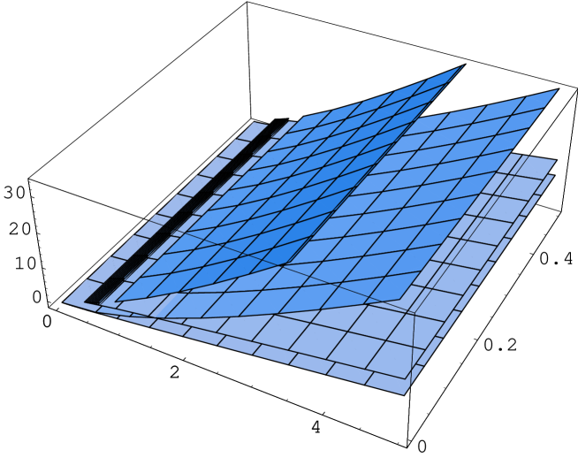
Figure 2: Plot of solutions $u_{r}(S,t),u_{1}(S,t),u_{2}(S,t)$ and $u_{3,1}(S,t),u_{3,2}(S,t)$ for the parameters $\sigma=0.4,~{}|c|=0.5,q=-4,b=1.0,d=0$. The variables $S,t$ lie in intervals $S\in(0.,5.)$ and $t\in[0,0.5]$. All invariant solutions change slowly in $t$-direction.

If we keep in mind that $z=\log S-\frac{\sigma^{2}}{8}t$ and $u(S,t)=S~{}v(z)$ we can represent the complete set of exact invariant solution of equation (2.7). The solution (3.2) gives rise to an invariant solution $u_{r}(S,t)$ in the form

$$u_{r}(S,t) = -\frac{1}{\omega\rho}S\left(1+c\,S^{-\frac{3}{2}}e^{\frac{3\sigma^{2}}{16}t}+{\sqrt{2\,c\,S^{-\frac{3}{2}}e^{\frac{3\sigma^{2}}{16}t}+c^{2}\,S^{-3}e^{\frac{3\sigma^{2}}{8}t}}}\right)^{-\frac{2}{3}}$$

$$- \frac{1}{\omega\rho}S{\left(1+c\,S^{-\frac{3}{2}}e^{\frac{3\sigma^{2}}{16}t}+{\sqrt{2\,c\,S^{-\frac{3}{2}}e^{\frac{3\sigma^{2}}{16}t}+c^{2}\,S^{-3}e^{\frac{3\sigma^{2}}{8}t}}}\right)}^{\frac{2}{3}}~{}~{}~{}~{}~{}$$

$$- \frac{2}{\omega\rho}S\log\left({\left(1+c\,S^{-\frac{3}{2}}e^{\frac{3\sigma^{2}}{16}t}+{\sqrt{2\,c\,S^{-\frac{3}{2}}e^{\frac{3\sigma^{2}}{16}t}+c^{2}\,S^{-3}e^{\frac{3\sigma^{2}}{8}t}}}\right)}^{-\frac{1}{3}}\right.$$

$$+ \left.{\left(1+c\,S^{-\frac{3}{2}}e^{\frac{3\sigma^{2}}{16}t}+{\sqrt{2\,c\,S^{-\frac{3}{2}}e^{\frac{3\sigma^{2}}{16}t}+c^{2}\,S^{-3}e^{\frac{3\sigma^{2}}{8}t}}}\right)}^{\frac{1}{3}}-2\right)+d~{}S+d_{2}$$

where $d,~{}d_{2}\in\mathbb{R}$, $c>0$. This solution was obtained and studied in [6]. We describe now other invariant solutions from the complete set of invariant solutions.

In case $c<0$ we can obtain correspondingly three real solutions if

$$S\geq\left(\frac{|c|}{2}\right)^{2/3}\exp{\left(\frac{\sigma^{2}}{8}t\right)}.$$ (3.64)

The first solution is represented by

$$u_{1}(S,t)=-\frac{1}{\omega\rho}S\left(\log{S}-\frac{\sigma^{2}}{8}t\right)-\frac{2}{\omega\rho}\,S\cos\left(\frac{2}{3}\,\arccos\left(1-|c|\,S^{-\frac{3}{2}}e^{\frac{3\sigma^{2}}{16}t}\right)\right)$$

$$-\frac{4}{3\omega\rho}\,S\log\left(1+2\,\cos\left(\frac{1}{3}\,\arccos\left(1-|c|\,S^{-\frac{3}{2}}e^{\frac{3\sigma^{2}}{16}t}\right)\right)\right)$$ (3.65)

$$-\frac{16}{3\omega\rho}\,S\log\left(\sin\left(\frac{1}{6}\,\arccos\left(1-|c|\,S^{-\frac{3}{2}}e^{\frac{3\sigma^{2}}{16}t}\right)\right)\right)+d~{}S+d_{2},$$

where $d,~{}d_{2}\in\mathbb{R}$, $c<0$. The second solution is given by the formula

$$u_{2}(S,t) = -\frac{1}{\omega\rho}S\left(\log{S}-\frac{\sigma^{2}}{8}t\right)-\frac{2}{\omega\rho}\,S\cos\left(\frac{2}{3}\pi+\frac{2}{3}\,\arccos\left(-1+|c|\,S^{-\frac{3}{2}}e^{\frac{3\sigma^{2}}{16}t}\right)\right)$$

$$- \frac{4}{3\omega\rho}\,S\log\left(1+2\,\cos\left(\frac{1}{3}\pi+\frac{1}{3}\,\arccos\left(-1+|c|\,S^{-\frac{3}{2}}e^{\frac{3\sigma^{2}}{16}t}\right)\right)\right)$$

$$- \frac{16}{3\omega\rho}\,S\log\left(\sin\left(\frac{1}{6}\pi+\frac{1}{6}\,\arccos\left(-1+|c|\,S^{-\frac{3}{2}}e^{\frac{3\sigma^{2}}{16}t}\right)\right)\right)+d~{}S+d_{2}.$$

where $d,~{}d_{2}\in\mathbb{R}$, $c<0$. The first and second solutions are defined for the variables under conditions (3.64). They coincide along the curve

$$S=\left(\frac{|c|}{2}\right)^{2/3}\exp{\left(\frac{\sigma^{2}}{8}t\right)}$$

and cannot be continued further. The third solution is defined by

$$u_{3,2}(S,t) = -\frac{1}{\omega\rho}S\left(\log{S}-\frac{\sigma^{2}}{8}t\right)$$

$$- \frac{2}{\omega\rho}\,S\cos\left(\frac{2}{3}\,\arccos\left(-1+|c|\,S^{-\frac{3}{2}}e^{\frac{3\sigma^{2}}{16}t}\right)\right)$$

$$- \frac{4}{3\omega\rho}\,S\log\left(-1+2\,\cos\left(\frac{1}{3}\,\arccos\left(-1+|c|\,S^{-\frac{3}{2}}e^{\frac{3\sigma^{2}}{16}t}\right)\right)\right)$$

$$- \frac{16}{3\omega\rho}\,S\log\left(\cos\left(\frac{1}{6}\,\arccos\left(-1+|c|\,S^{-\frac{3}{2}}e^{\frac{3\sigma^{2}}{16}t}\right)\right)\right)+d~{}S+d_{2},$$

where $d,~{}d_{2}\in\mathbb{R}$ and $S,t$ satisfied the condition (3.64).

In case $0<S<\left(\frac{|c|}{2}\right)^{\frac{2}{3}}\exp{\left(\frac{\sigma^{2}}{8}t\right)}$ the third solution can be represented by the formula

$$u_{3,1}(S,t) = -\frac{1}{\omega\rho}S\left(\log{S}-\frac{\sigma^{2}}{8}t\right)$$

$$- \frac{2}{\omega\rho}\,S\cosh\left(\frac{2}{3}{\rm arccosh}\left(-1+|c|\,S^{-\frac{3}{2}}e^{\frac{3\sigma^{2}}{16}t}\right)\right)$$

$$- \frac{16}{3\,\omega\rho}\,S\log\left(\cosh\left(\frac{1}{6}{\rm arccosh}\left(-1+|c|\,S^{-\frac{3}{2}}e^{\frac{3\sigma^{2}}{16}t}\right)\right)\right)$$

$$- \frac{4}{3\,\omega\rho}\,S\log\left(-1+2\,\cosh\left(\frac{1}{3}{\rm arccosh}\left(-1+|c|\,S^{-\frac{3}{2}}e^{\frac{3\sigma^{2}}{16}t}\right)\right)\right)$$

$$+ d~{}S+d_{2},$$

where $d,~{}d_{2}\in\mathbb{R}.$ The solution $u(S,t)$ (3.2) and the third solution given by $u_{3,1}$, $u_{3,2}$ (3.2),(3.2) are defined for all values of variables $t$ and $S>0$. They have a common intersection curve of the type $S={\rm const.}~{}\exp({\frac{\sigma^{2}}{8}t})$. The typical behavior of all these invariant solutions is represented in Fig. 2.

The previous results we summarize in the following theorem which describes the set of invariant solutions of equation (2.7).

Theorem 3.4

The invariant solutions of equation (2.7) can be defined by the set of first order ordinary differential equations listed in Theorem 3.2.
If moreover the parameter $q=-4$, or equivalent in the substitution (3.22) we chose $a=-\sigma^{2}/8$ then the complete set of invariant solutions of (2.7) can be found exactly. This set of invariant solutions is given by formulas (3.2)–(3.2) and by solutions

$$u(S,t)=d~{}S,~{}~{}u(S,t)=\frac{3}{b}~{}S~{}(\log{S}-\sigma^{2}\frac{t}{8}),$$

$$~{}~{}u(S,t)=-\frac{1}{b}~{}S~{}(\log{S}-\sigma^{2}\frac{t}{8}),$$

where $d$ is an arbitrary constant. This set of invariant solutions is unique up to the transformations of the symmetry group $G_{\Delta}$ given by Theorem 3.1.

The solutions $u_{r}(S,t)$, (3.2), $u_{1}(S,t)$, (3.65), $u_{2}(S,t)$, (3.2), $u_{3,1}(S,t)$ ,(3.2), $u_{3,2}(S,t)$ (3.2), have no one counterpart in a linear case. If in the equation (2.7) the parameter $\rho=0$ equation becomes linear. If the parameter $\rho\to 0$ then equation (2.7) and correspondingly equation (3.18) will be reduced to the linear Black-Scholes equation but solutions (3.2)-(3.2) which we obtained here will be completely blown up by $\rho\to 0$ because of the factor $1/b=1/(\omega\rho)$ in the formulas (3.2)-(3.2). This phenomena was described as well in [6], [8] where the solution $u_{r}(S,t)$ was studied and for the complete set of invariant solutions of equation (3.18) with $k=1$ in [5].

4 Properties of solutions and parameter-sensitivity

We study the properties of solutions, keeping in mind that because of the symmetry properties (see Theorem 3.1) of the equation (2.7) we can add to each solution a linear function of $S$.

4.1 Dependence on the constant $c$ and terminal payoff

First we study the dependence of the solution $u_{2}$ on the arbitrary constant $c$. The constant $c$ is the first constant of integration of the ordinary differential equations (3.31), (3.32). This dependence is illustrated in Figure 4.

Figure 3: Plot of solutions $u_{2}(S,t)$ where $~{}|c|=0.01,1.,5.,10.,20.,\sigma=0.4,q=-4$, $b=1.0,d=0$. The variables $S$ lie in intervals $S\in(0.,15.)$ and $t=1.$.

The curves going from up to down with the growing value of the parameter $|c|$.

Figure 4: Plot of solutions $u_{3}(S,t)$ where $|c|=0.01,1.,5.,10.,20.,\sigma=0.4,q=-4$, $b=1.0,d=0$. The variables $S$ lie in intervals $S\in(0.,15.)$ and $t=1.$.

The curves going from up to down with the growing value of the parameter $|c|$.

We see on Fig. 4 that for different values of the constant $c$ the domains of the solutions are different. The dependence of the solutions $u_{3,1},u_{3,2}(S,t)$ on the constant $c$ is exemplified in Figure 4.

We obtain a typical terminal payoff function for the solutions (3.2)-(3.2) if we just fix $t=T$. By changing the value of the constant $c$ and by adding a linear function of $S$ we are able to modify terminal payoff function for the solutions. Hence we can approximate typical payoff profiles of financial derivatives quite well.

4.2 Dependence on time

All solutions depend weakly on time because of the substitution (3.49) all invariant solutions depends on the combination $\sigma^{2}t$. As long as we take the volatility $\sigma$ to be small we obtain a dampened dependence of the solutions on time.

In Fig. 5 we can see this dependence for examples of the solution $u_{3,1}(S,t),u_{3,2}(S,t)$.

Figure 5: Plot of solutions $u_{3,1}(S,t),u_{3,2}(S,t)$ for the parameters $\sigma=0.4,~{}|c|=10.,q=-4,b=1.0,d=0$. The variables $S$ lie in intervals $S\in(0.,15.)$ and $t=0.01,1.,5.,10.,20.$.

The highest level corresponds to $t=0.01$ and the lowest to $t=20.$.

4.3 Dependence on the parameter $\rho$

All solutions found in this paper have the form

$$u(S,t)=w(S,t)/\rho,$$ (4.69)

where $w(S,t)$ is a smooth function of $S,t$. Hence the function $w(S,t)$ solves the equation (2.7) with $\rho=1$,

$$w_{t}+\frac{\sigma^{2}S^{2}}{2}\frac{w_{SS}}{(1-Sw_{SS})^{2}}=0.$$ (4.70)

Because of this relation any $\rho$-dependence of invariant solutions of (2.7) trivial. In particular, if the terminal conditions are fixed, $u(S,T)=h(S)$, then the value $u(S,t)$ will increase if the value of the parameter $\rho$ increases. This dependence of hedge costs on the position of the large trader on the market is very natural.

4.4 Dependence on the asset price $S$

In practice one use often delta-hedging to reduce the sensitivity of a portfolio to the movements of an underlying asset. Hence it is important to know the value $\Delta$ defined by $\Delta=\frac{\partial u}{\partial S},$ where $u$ denotes the value of the derivative product or of a portfolio. Using the exact formulas for the invariant solutions we can easily calculate $\Delta$ as a function of $S$ and $t$. The $\Delta$ corresponding to the solution $u_{2}$ is presented in Fig. 7

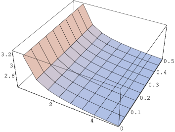
Figure 6: Plot of $\Delta$ for $u_{2}(S,t)$ and $\sigma=0.4,~{}|c|=1.,q=-4,b=1.0,d=0$. The variables lie in intervals $S\in(0.,5.)$ and $t=[0.,0.5]$.

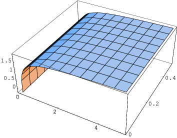
Figure 7: Plot of the $\Delta$ for $u_{3,1}(S,t),u_{3,2}(S,t)$ and $\sigma=0.4,~{}|c|=1.,q=-4,b=1.0,d=0$. The variables lie in intervals $S\in(0.,5.)$ and $t\in[0.01,0.5]$.

The $\Delta$ of the solution $u_{3,1},u_{3,2}$ is represented on the Fig. 7.
We see in both cases the strong dependence on $S$ for small value of $S$. If $S\to\infty$, in both cases the $\Delta$ tends to a constant which is independent of time and the constant $c$.

4.5 Asymptotic behavior of invariant solutions

If $S$ is large enough we have four well defined solutions $u_{r}(S,t)$, $u_{1}(S,t)$, $u_{2}(S,t)$, $u_{3,2}(S,t)$. The asymptotic behavior solutions $u_{r}(S,t)$ from (3.2) and $u_{1}$ from (3.65) coincides in the main terms as $S\to\infty$ and is given by the formula

$$u_{r}(S,t),~{}u_{1}(S,t)\sim\frac{1}{b}\left(3S\ln S+{\rm const.}S+{\cal O}(S^{-1/2})\right)$$ (4.71)

The exact formula for the asymptotic behavior of the function $u_{1}(S,t)$ for $S\to\infty$ is given by

$$u_{1}(S,t) \sim \frac{3}{b}\,S\log(S)+\frac{1}{b}S\left(4\,\log(3)-2-\frac{8}{3}\,\log\left(\frac{2}{|c|}\right)-\frac{3}{8}\sigma^{2}\,t\right)$$ (4.72)

$$+ \frac{2^{4}}{3^{3}b}\,|c|\,e^{\frac{3\,{\sigma}^{2}\,t}{16}}\,S^{-\frac{1}{2}}+{\cal O}\left(S^{-\frac{5}{4}}\right).$$

We see that for $S\to\infty$, the main term does not depend on time or on the value of the constant $c$. Moreover, this term cannot be changed by adding a linear function of $S$ to the solution.

The main terms of the solutions $u_{2}(S,t)$ from (3.2) and $u_{3,2}$ from (3.2) behave similar to each other as $S\to\infty$; this behavior is given by the formulas

$$u_{2}(S,t) \sim \frac{1}{b}\left(1+\frac{2}{3}\,\log\left(\frac{2^{7}}{3^{3}|c|}\right)\right)\,S$$

$$+ \frac{2^{3}}{3b}\,\sqrt{\frac{2|c|}{3}}\,e^{\frac{3\,{\sigma}^{2}\,t}{32}}\,S^{\frac{1}{4}}-\frac{2^{3}}{3^{3}b}\,|c|\,e^{\frac{3\,{\sigma}^{2}\,t}{16}}\,S^{-\frac{1}{2}}+{\cal O}\left(S^{-\frac{5}{4}}\right).$$

and

$$u_{3,2}(S,t) \sim \frac{1}{b}\left(1+\frac{2}{3}\,\log\left(\frac{2^{7}}{3^{3}|c|}\right)\right)\,S$$ (4.74)

$$- \frac{2^{3}}{3b}\,\sqrt{\frac{2|c|}{3}}\,e^{\frac{3\,{\sigma}^{2}\,t}{32}}\,S^{\frac{1}{4}}-\frac{2^{3}}{3^{3}b}\,|c|\,e^{\frac{3\,{\sigma}^{2}\,t}{16}}\,S^{-\frac{1}{2}}+{\cal O}\left(S^{-\frac{5}{4}}\right).$$ (4.75)

Note that the main term in formulas (4.5) and (4.74) depends on $S$ linearly and has a coefficient which depends on the constant $c$ only. Hence we can change the asymptotic behavior of the solutions $u_{2}(S,t)$ and $u_{3,1}(S,t)$, $u_{3,2}(S,t)$ by simply adding a linear function of $S$ to the solutions.

For $S$ in a neighborhood of $S\to 0$ there exist just two non trivial real invariant solutions of equation (2.7), i.e. the known solution $u_{r}(S,1)$ and the new solution $u_{3,1}(S,t)$. Using the exact formulas for the last solution we retain the first term and obtain as $S\to 0$ for the solution $u_{3,1}(S,t)$

$$u_{3,1}(S,t)\sim\frac{-14}{b}~{}S\ln\left(S\right)+{\cal O}\left(S\right).$$ (4.76)

The main term in this formula do not depend on $t$ or constant $c$ and can be changed by adding a linear function of $S$ to the solution.

5 Conclusion

In this paper we have obtained explicit solutions for the equation (2.7) and studied their analytical properties. These solutions are useful for a number of reasons. To begin with, while the payoffs of these similarity solutions cannot be chosen arbitrary, the payoffs can be modified using embedded constants to tailor a given portfolio reasonably well. For some values of the parameters $c,d$ we obtain a payoff typical for futures, for other values $c,d$ the payoff is very similar to the form of calls (see Figure 4 and Figure 4). Moreover, the explicit solutions can be used as benchmark for different numerical methods.

An important difference between the case of the linear Black-Scholes equation and these nonlinear cases can be noticed if we consider the asymptotic for $S\to\infty$. In the linear case the price of a Call option satisfies $u(S,t)\to{\rm const}\cdot S$. In the nonlinear case the families of similarity solutions $u_{2}$ and $u_{3}$ which approximate the payoff of a Call option well on a finite interval $[0,\bar{S}]$, grow faster than linear as $S\to\infty$; see the formulas (4.5) and (4.74) for details. This reflects the fact that in illiquid markets option hedging is more expensive than in the standard case of perfectly liquid markets.

6 Acknowledgements

The authors are grateful to Albert N. Shiryaev for the interesting and fruitful discussions.

References

- [1] P. Bank and D. Baum. Hedging and portfolio optimization in financial markets with a large trader. Math. Finance, 14:1–18, 2004.
- [2] G. Barles and M. Soner. Option pricing with transaction costs and a nonlinear Black-Scholes equation. Finance Stoch., 2:369–397, 1998.
- [3] D. Becherer. Utility indifference hedging and valuation via reaction-diffusion systems. R. Soc. Lond. Proc. Ser. A Math. Phys. Eng. Sci., 460:27–51, 2004.
- [4] M. V. Bobrov. The fair price valuation in illiquid markets. Master’s Thesis in Financial Mathematics, Technical report IDE0738, Halmstad University, Sweden, 2007.
- [5] L. A. Bordag. On the valuation of a fair price in case of an non perfectly liquid market. Proceedings of the Workshop on Mathematical Control Theory and Finance, Lisbon, 10-14 April, 2007. (working paper version entitled ‘Symmetry reductions of a nonlinear model of financial derivatives’, arXiv:math.AP/0604207, 09.04.2006).
- [6] L. A. Bordag and A. Y. Chmakova. Explicit solutions for a nonlinear model of financial derivatives. International Journal of Theoretical and Applied Finance, 10:1–21, 2007. No. 1.
- [7] U. Cetin, R. Jarrow, and P. Protter. Liquidity risk and arbitrage pricing theory. Finance Stoch., 8:311–341, 2004.
- [8] A. Y. Chmakova. Symmetriereduktionen und explizite Lösungen für ein nichtlineares Modell eines Preisbildungsprozesses in illiquiden Märkten. PhD thesis, BTU Cottbus, Germany, 2005.
- [9] R. Frey. Perfect option replication for a large trader. Finance Stoch., 2:115–148, 1998.
- [10] R. Frey. Market illiquidity as a source of model risk in dynamic hedging. In R. Gibson, editor, Model Risk, pages 125–136. Risk Publications, London, 2000.
- [11] R. Frey and P. Patie. Risk management for derivatives in illiquid markets: a simulation study. In K. Sandmann and P. Schönbucher, editors, Advances in Finance and Stochastics. Springer, Berlin, 2002.
- [12] R. Frey and A. Stremme. Market volatility and feedback effects from dynamic hedging. Math. Finance, 7(4):351–374, 1997.
- [13] Nail H. Ibragimov. Elementary Lie Group Analysis and Ordinary Differential Equations. John Wiley & Sons, Chichester, USA, 1999.
- [14] M. Jandačka and D. Ševčovi ̌c. On the risk-adjusted pricing-methodology-based valuation of vanilla options and explanation of the volatility smile. Journal of Applied Mathematics, 3:253–258, 2005.
- [15] R.A. Jarrow. Derivative securities markets, market manipulation and option pricing theory. J. Finan. Quant. Anal., 29:241–261, 1994.
- [16] Robin Stanley Johnson. Singular perturbation theory:. Mathematical and analytical techniques with applications to engineering. Springer, New York, 2004.
- [17] Sophus Lie. Vorlesungen über Differentialgleichungen mit bekannten infinitesimalen Transformationen. Teubner, Leipzig, 1912.
- [18] H. Liu and J. Yong. Option pricing with an illiquid underlying asset market. Journal of Economic Dynamics and Control, 29(12):2125–2156, 2005.
- [19] M. Musiela and T. Zariphopoulou. An example of indifference prices under exponential preferences. Finance and Stochastics, 8:229–239, 2004.
- [20] P. J. Olver. Application of Lie groups to differential equations. Springer-Verlag, New York, USA, 1986.
- [21] E. Platen and M. Schweizer. On feedback effects from hedging derivatives. Math. Finance, 8:67–84, 1998.
- [22] P. Protter. Stochastic Integration and Differential Equations: A New Approach. Applications of Mathematics. Springer, Berlin, 1992.
- [23] P. Schönbucher and P. Wilmott. The feedback-effect of hedging in illiquid markets. SIAM J. Appl. Math., 61:232–272, 2000.
- [24] N. Sergeeva. The feedback effects in illiquid markets, hedging strategies of large traders. Master’s Thesis in Financial Mathematics, Technical report IDE0741, Halmstad University, Sweden, 2007.
- [25] R. Sircar and G. Papanicolaou. General Black-Scholes models accounting for increased market volatility from hedging strategies. Appl. Math. Finance, 5:45–82, 1998.