Non-linear optics with two trapped atoms

Abstract

We show theoretically that two atomic dipoles in a resonator constitute a non-linear medium, whose properties can be controlled through the relative position of the atoms inside the cavity and the detuning and intensity of the driving laser. We identify the parameter regime where the system operates as a parametric amplifier, based on the cascade emission of the collective dipole of the atoms, and determine the corresponding spectrum of squeezing of the field at the cavity output. This dynamics could be observed as a result of self-organization of laser-cooled atoms in resonators.

I Introduction

Quantum light sources are an essential element for implementations of quantum information processing and secure telecommunication with quantum optical systems qic ; Briegel98 ; Kraus ; Braunstein05 . Experiments have demonstrated several remarkable milestones, thereby opening promising perspectives for implementing controlled generation of quantum light Walther04 ; Kimble03 ; Kimble04 ; Rempe02 ; Kuhn ; Lukin04 ; Kuzmich06 ; Polzik06 ; Grangier05 ; Grangier06 ; Monroe04 ; Weinfurter06 . Besides, these studies touch on the fundamental question of how macroscopic nonlinear phenomena emerge from the dynamics of quantum systems Savels07 . A paradigmatic example is the optical parametric amplifier WallsMilburn . This system is usually realized with non-linear crystals in resonators, where the medium response is characterized by the dependence of the macroscopic polarization on the electric field, and where symmetries of the crystal can enhance a certain nonlinear response over others Armstrong62 ; Boyd . On the other hand, recent theoretical works pointed out that a single atom in a suitable setup can constitute an efficient non-linear optical medium operating in the quantum regime Imamoglu97 ; kimbleParkins ; Morigi06 ; Vitali06 . A question, which naturally emerges from these works, is how these dynamics scale up to a macroscopic non-linear medium, and in particular what is the microscopic building block exhibiting the essential symmetries controlling the order of the medium susceptibility.

In this article we study the non-linear response of a medium constituted by two dipoles confined along the axis of an optical resonator, and transversally driven by a laser, in a configuration like the one depicted in Fig. 1. At certain interatomic distances the state of the field at the cavity output can exhibit non-classical features. In particular, we show that the system response can be switched from a parametric amplifier to a Kerr medium, just by varying the intensity of the laser field. The validity of our analytical predictions are verified by numerical simulations which take into account the internal dynamics of the atoms and their coupling with the quantized mode of the resonator. The effect of atomic vibrations on the field at the cavity output is estimated using a semiclassical model for the atomic motion. Finally, we discuss the possibility of obtaining such patterns, operating in the quantum regime, as the result of self-organization of laser-cooled atoms in the resonator field Domokos02 ; Asboth05 .

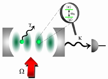
Figure 1: Two atoms are confined inside a high-finesse optical resonator, their dipoles are driven by a laser and couple to a mode of the cavity. The quantum state of the field at the cavity output can be controlled by the interatomic distance inside the resonator and the laser intensity and detuning. A detecting apparatus measures the field at the cavity output.The parameters are defined in Sec. II.

This article is organized as follows. In Sec. II the model is introduced and the basic properties are discussed. In Sec. III the response of the atomic medium is determined as a function of the atomic position inside the resonator, when the atoms are driven by a laser. The steady state of cavity and atoms is determined for the specific parameter regime in which the system behaves as an optical parametric amplifier. In Sec. IV we consider the effect of the center of mass motion on the cavity field by means of a semiclassical model. In Sec. V we summarize the results and discuss some outlooks. The appendices provide details of the calculations presented in Sec. III and Sec IV.

II The theoretical model

We assume two identical atoms of mass $M$, which are confined inside a standing-wave cavity, and localized at the position $x_{1}$ and $x_{2}$, respectively, along the cavity axis. We denote by $p_{1}$ and $p_{2}$ the corresponding momenta, and by $H_{\rm mec}$ the Hamiltonian determining the dynamics of the center of mass in absence of the coupling with the electromagnetic field, which has the form

$$H_{mec} = \frac{p_{1}^{2}}{2M}+\frac{p_{2}^{2}}{2M}+V(x_{1},x_{2})$$ (1)

with $V(x_{1},x_{2})$ an external potential, which localizes the atoms at their equilibrium positions such that they undergo small vibrations with respect to the cavity-mode wavelength. The relevant internal degrees of freedom of the atoms are the ground state $|g\rangle$ and the excited state $|e\rangle$ of a dipole transition with dipole moment ${\bf d}$, which is at frequency $\omega_{0}$. The dipoles are driven by a transverse laser field at frequency $\omega_{L}$ and couple to a mode of the resonator at frequency $\omega_{c}$ and wave vector $k$, as displayed in Fig. 1. A detecting apparatus measures the field at the cavity output.

II.1 Master Equation

In the reference frame rotating at the laser frequency the coherent dynamics of the atoms and cavity mode is described by the Hamiltonian $H=H_{mec}+H_{at}+H_{cav}+H_{cav-at}+H_{L}$. The terms

$$H_{at} = -\hbar\Delta\sum_{j=1,2}\sigma^{\dagger}_{j}\sigma_{j}$$ (3)

$$H_{cav} = -\hbar\delta_{c}a^{{\dagger}}a$$ (4)

describe the system dynamics in absence of coupling with the electromagnetic field. Here, $\Delta=\omega_{L}-\omega_{0}$ and $\delta_{c}=\omega_{L}-\omega_{c}$ are the detunings of the laser from the dipole and from the cavity frequency, respectively, $\sigma_{j}=\left|g\right\rangle_{j}\left\langle e\right|$ the lowering operator of the atom $j$, $\sigma^{\dagger}_{j}$ its adjoint, and $a$ and $a^{{\dagger}}$ are the annihilation and creation operators of a photon of the cavity mode. The terms

$$H_{L} = \hbar\Omega\sum_{j=1,2}\left(\sigma^{\dagger}_{j}+\sigma_{j}\right),$$ (5)

$$H_{at-cav} = \hbar\sum_{j=1,2}g(x_{j})\left(a^{{\dagger}}\sigma_{j}+\sigma^{\dagger}_{j}a\right)$$ (6)

describe the interaction of the dipoles with the cavity and laser fields, respectively, with $\Omega$ the laser Rabi frequency and $g(x_{j})$ the cavity vacuum coupling strength at $x_{j}$, with $g(x_{j})=g\cos(kx_{j})$. In Eq. (5) the laser wave vector is orthogonal to the cavity axis.

Coupling to the external environment gives rise to dissipation and decoherence, which is described by spontaneous emission of the excited state at rate $\gamma$ and by cavity decay at rate $\kappa$. The dynamics of the density matrix $\rho$ of the cavity and atomic degrees of freedom is given by the master equation

$$\frac{\partial}{\partial t}\rho = -\frac{\rm i}{\hbar}\left[H,\rho\right]+{\cal L}_{\kappa}\rho+{\cal L}_{\gamma}\rho$$ (7)

$$\equiv {\cal L}\rho$$ (8)

where

$${\cal L}_{\kappa}\rho=\kappa\left(2a\rho a^{\dagger}-a^{\dagger}a\rho-\rho a^{\dagger}a\right)$$ (9)

is the superoperator which describes noise due to cavity decay, and

$${\cal L}_{\gamma}\rho=\sum_{j=1,2}\frac{\gamma}{2}\left(2\sigma_{j}\tilde{\rho}_{j}\sigma_{j}^{\dagger}-\sigma_{j}^{\dagger}\sigma_{j}\rho-\rho\sigma_{j}^{\dagger}\sigma_{j}\right)$$ (10)

is the superoperator which describes the quantum noise due to spontaneous emission. In the superoperator (10) the term $\tilde{\rho}_{j}$ accounts for the mechanical effect of the spontaneously emitted photon on the atom in $x_{j}$, see for instance Zippilli05 .

II.2 Multi-photon processes and atomic patterns

It is instructive to consider the dynamics in terms of the collective states of the dipole. We denote by $|+\rangle$ and $|-\rangle$ the Dicke symmetric and antisymmetric states, respectively, with $|\pm\rangle=(|eg\rangle\pm|ge\rangle)/\sqrt{2}$, and rewrite the interaction of the atoms with laser and cavity mode in terms of the operators

$$S_{\pm}=(\sigma_{1}\pm\sigma_{2})/\sqrt{2}.$$ (11)

In this representation, the laser-atom interaction, Eq. (5), is rewritten as

$$H_{L}=\hbar\sqrt{2}\Omega S_{+}+{\rm H.c.}$$ (12)

while the atom-cavity interaction term, Eq. (6), can be decomposed as $H_{at-cav}=H_{+}+H_{-}$, with

$$H_{\pm}=\hbar g_{\pm}(x_{1},x_{2})\left(aS_{\pm}^{\dagger}+a^{\dagger}S_{\pm}\right)$$ (13)

and

$$g_{\pm}(x_{1},x_{2})=\frac{g}{\sqrt{2}}\left(\cos(kx_{1})\pm\cos(kx_{2})\right).$$ (14)

This decomposition highlights the relevant cavity-atom dynamics, which depend on the relative atomic position. The term $H_{-}$ describes the coupling of the cavity mode with the Dicke anti-symmetric state, and it vanishes when the interatomic distance $d=x_{2}-x_{1}$ is an integer multiple of the cavity wavelength $\lambda=2\pi/k$. We denote the corresponding atomic configuration as ”$\lambda$-spaced pattern”. The term $H_{+}$ describes the coupling of the cavity mode with the Dicke symmetric state and it vanishes when $d$ is an odd multiple of $\lambda/2$. We denote the corresponding atomic configuration as ”$\lambda/2$-spaced pattern” Below we discuss the corresponding dynamics in detail.

II.2.1 $\lambda$-spaced pattern.

We first consider the case in which the interatomic distance is an integer multiple of $\lambda$. For this configuration, at steady state and for large cooperativities, the atoms are in the ground state and the cavity mode is in a coherent state whose amplitude is determined by the laser intensity Zippilli04 ; Alsing92 . This behaviour can be understood in terms of the coherent buildup of a cavity field, such that its phase is opposite to the driving field. As a result, the atomic dipole is not excited, even if the cavity mode is in a coherent state with a finite number of photons. When two or more atoms are present inside the resonator, this situation can be achieved when the atoms scatter in phase into the cavity modes, i.e., when they are arranged in a $\lambda$-spaced pattern. The coherent scattering processes which two atoms undergo are sketched in Fig. 2(a) in the Dicke basis, showing that the antisymmetric state $|-\rangle$ remain always decoupled from the coherent dynamics. Here, one identifies the suppression of excitation of the atoms at steady state as due to interference between the excitation path $|gg,n\rangle\to|+,n\rangle$, driven by the laser, and the excitation path $|gg,n+1\rangle\to|+,n\rangle$, driven by the cavity. Figure 2(a) displays also the other higher-order processes. In particular, we note the processes which lead to the excitation of the state $|ee,n\rangle$ by the absorption of two laser photons, followed by emission of pair of photons into the cavity. These processes are expected to give rise to squeezing of the coherent state of the cavity field. We note that squeezed-coherent radiation has been predicted in the resonance fluorescence of an atomic crystal, at wave vectors such that the Bragg condition of the atomic crystal is equivalent to the $\lambda$-spaced pattern here discussed Vogel85 . Finally, we note that the formation of $\lambda$-patterns of laser-cooled atoms inside of resonators has been predicted as the result of a self-organizing process Domokos02 ; Asboth05 , and features of the field at the cavity output, associated with their formation, have been measured in Chan03 ; Black03 . Theoretical works have shown that these patterns can be also stable in the strong coupling regime, under the condition, in which atomic excitation is suppressed and the cavity field is in a coherent state Zippilli04 ; Asboth04 .

II.2.2 $\lambda/2$-spaced pattern.

We now analyze the case, when the interatomic distance is an odd multiple of $\lambda/2$, such that $H_{+}=0$. In this case the atomic ground state couples via the laser to the Dicke symmetric state $|+\rangle$, and via the cavity to the antisymmetric state $|-\rangle$, as depicted in Fig. 2(b). Hence, when the laser drives the atoms well below saturation,the cavity is empty Zippilli04 . In fact, in this limit the two atoms scatter the laser photons with opposite phase into the cavity and the resulting field vanishes due to destructive interference. Figure 2(b) shows, however, that the cavity mode can be pumped by higher-order processes, which excite the state $|ee,0\rangle$. In this regime, the collective dipole can emit photons in pairs into the cavity mode. These processes are expected to give rise to squeezing of the state of the cavity field. We note that squeezed radiation has been predicted in the resonance fluorescence of an atomic crystal, at wave vectors such that the Bragg condition of the atomic crystal is equivalent to the $\lambda/2$-spaced pattern here discussed Vogel85 . In this paper we will investigate the quantum state of the light in presence of a high-finesse cavity when the atoms are initially in a $\lambda/2$ spaced pattern, and determine the dynamics resulting from the competition between coherent processes and noise, such as cavity decay, spontaneous emission, and atomic vibrations at the equilibrium positions.

Figure 2: Sketch of the coherent scattering processes between the collective states of two atomic dipoles driven by a laser and coupled to the cavity mode, when (a) the interatomic distance $d$ is an integer multiple of the cavity-mode wavelength $\lambda$, and (b) when $d$ is an odd multiple of $\lambda/2$. The states $|J,n\rangle$ are the Dicke states of the two dipoles $|J\rangle$ at $n$ cavity photons, where $|J\rangle=|gg\rangle,|\pm\rangle~{},|ee\rangle$, and $|\pm\rangle=(|eg\rangle\pm|ge\rangle)/\sqrt{2}$. The arrows labeled by $\Omega$ ($g_{\pm}$) indicate the transitions driven by the laser (the cavity mode).

III Non-linear response of two trapped atoms

In this section, starting from Eq. (7) we derive the equation describing the effective dynamics of the cavity mode in the limit of large atom-laser detuning $|\Delta|\gg g,\Omega,|\delta_{c}|,\gamma,\kappa$. In this analysis we neglect the effect of atomic motion, and identify the parameter regime in which the system operates as a parametric amplifier. The prediction of the analytical model are compared with the results of a numerical simulation, which evaluate the cavity mode state by solving Eq. (7).

III.1 Effective Hamiltonian

We derive the effective Hamiltonian $H_{\rm eff}$ for the coherent cavity dynamics at fourth order in the expansion in the small parameters $g/|\Delta|$, $\Omega/|\Delta|$. In the Hilbert subspace subtended by the states $|gg,n\rangle$, with $n$ the number of cavity photons, it has the form

$$H_{\rm eff} = \left(\bar{\theta}-\delta_{c}\right)a^{{\dagger}}a+\bar{\beta}\left(a^{\dagger}+a\right)$$ (15)

$$\bar{\chi}a^{\dagger}a^{\dagger}aa+\frac{\bar{\alpha}}{2}\left({a^{\dagger}}^{2}+{a}^{2}\right),$$

where

$$\bar{\theta} = \frac{g_{+}^{2}\left(x_{1},x_{2}\right)+g_{-}^{2}\left(x_{1},x_{2}\right)}{\Delta}$$ (16)

$$\bar{\beta} = \frac{\sqrt{2}\Omega}{\Delta}g_{+}\left(x_{1},x_{2}\right)$$ (17)

$$\bar{\chi} = \frac{1}{\Delta^{3}}\left[g_{+}^{2}\left(x_{1},x_{2}\right)-g_{-}^{2}\left(x_{1},x_{2}\right)\right]^{2}$$ (18)

$$\bar{\alpha} = \frac{2\Omega^{2}}{\Delta^{3}}\left[g_{+}^{2}\left(x_{1},x_{2}\right)-g_{-}^{2}\left(x_{1},x_{2}\right)\right]$$ (19)

Here, $\bar{\theta}$ is the a.c.-Stark shift experienced by the cavity field due to the interaction with the atoms, the term $\bar{\beta}$ comes from the $H_{+}$ term, Eq. (13), and results from the two-photon transitions coupling the photon states $|n\rangle$ and $|n\pm 1\rangle$, see Fig. 2(a). The amplitude $\bar{\alpha}$ is the strength of the effective nonlinear pumping of the cavity field which gives rise to a $\chi^{(2)}$ nonlinearity, typical of a degenerate parametric amplifier WallsMilburn . This term is the sum of two contributions, which are weighted by $g_{+}$ and $g_{-}$, respectively, and which represent the coherent sum of the four-photon processes coupling the states $|gg,n\rangle\to|gg,n\pm 2\rangle$ and depicted in Fig. 2(a) and (b). Finally, the amplitude $\bar{\chi}$ is the a.c-Stark shift associated with four-photon processes, where two cavity photon are virtually absorbed and then emitted along the transition $|gg,n\rangle\to|ee,n-2\rangle$. This term is present in both patterns, and gives rise to the $\chi^{(3)}$ nonlinearity typical of a Kerr medium.

The form of Hamiltonian (15) highlights how the two patterns we considered, $\lambda$- and $\lambda/2$-spaced, contribute to the various nonlinear processes. We first notice that in presence of only one atom (when, e.g., $g(x_{2})=0$) the terms $\bar{\alpha}$ and $\bar{\chi}$ trivially vanish: these types of nonlinearities can be clearly generated only when both atoms couple to the cavity mode. Then, one observes that the two patterns gives rise to different nonlinear dynamics. In the $\lambda$-spaced pattern, for instance, all terms in Eq. (15) contribute to determine the coherent dynamics of the cavity mode. While the linear shift $\bar{\theta}$ can be set to zero by properly choosing the detuning $\delta_{c}$, on the other hand the linear term scaling with $\bar{\beta}$ is dominant, and one reasonably expects that it will determine the cavity steady state.

When the atoms are distributed in a $\lambda/2$-spaced pattern, the linear drive in Hamiltonian (15) vanishes, i.e., $\bar{\beta}=0$, while the only terms which contribute to the coherent dynamics are at fourth order in the perturbative expansion. Two possible scenarios can be here identified. (i) When the laser drive is much weaker than the cavity coupling, $\Omega\ll g$, then $|\bar{\chi}|\gg|\bar{\alpha}|$ and the dynamics will be basically equivalent to a Kerr medium as in Imamoglu97 , whereby in our case the Kerr nonlinearity emerges from the interaction of the cavity field with the collective dipole of the atoms. (ii) When the laser drive is much stronger than the cavity coupling, $\Omega\gg g$, then $|\bar{\chi}|\ll|\bar{\alpha}|$ and the dynamics will be essentially equivalent to the one in a $\chi^{(2)}$-medium. This is the case on which we focus in the rest of this article.

III.2 Realization of a $\chi^{(2)}$ medium

We now consider Hamiltonian (15) when the atoms are localized at the antinodes of the cavity modes in a $\lambda/2$-spaced pattern, i.e., when $\bar{\beta}=0$, and when $\Omega\gg g$, i.e., $|\bar{\alpha}|\gg|\bar{\chi}|$. Setting ${\delta}_{c}=\bar{\theta}$, the effective coherent dynamics of the cavity mode is described by Hamiltonian $H_{\rm eff}\approx H^{\prime}$, with

$$H^{\prime}=\frac{\bar{\alpha}}{2}\left(a^{2}+a^{{\dagger}^{2}}\right)$$ (20)

and $\bar{\alpha}=\alpha$, where now

$$\alpha=-\frac{4\Omega^{2}g^{2}}{\Delta^{3}}$$ (21)

A master equation for the reduced density matrix $\varrho$ of the cavity mode can be derived from Eq. (7), which takes the form

$$\frac{\partial}{\partial t}\varrho=-\frac{\rm i}{\hbar}\left[H^{\prime},\varrho\right]+{\cal L}_{\kappa}\varrho+\tilde{\cal L}_{\gamma}\varrho$$

where superoperator ${\cal L}_{\kappa}$ is defined in Eq. (9), while

$$\tilde{\cal L}_{\gamma}\varrho=\frac{\gamma^{\prime}}{2}(2a\varrho a^{\dagger}-a^{\dagger}a\varrho-\varrho a^{\dagger}a)$$ (22)

describes the damping of the cavity mode via spontaneous emission, with $\gamma^{\prime}\approx\gamma g^{2}/\Delta^{2}$.

When $\alpha>\kappa+\gamma^{\prime}$, Eq. (III.2) predicts that the energy of the cavity mode increases exponentially as a function of time. Clearly, this exponential increase is a good approximation only for short times, when the number of photons inside the cavity mode still warrants the validity of the perturbative expansion, while for longer times the dynamics will be determined by competition with other processes which we neglected in the derivation.

When $\kappa+\gamma^{\prime}>\alpha$, a steady state solution exists, and the corresponding stationary average photon number is

$$n_{0}\equiv\left\langle a^{{\dagger}}a\right\rangle_{\rm St}=\frac{1}{2}\frac{\alpha^{2}}{\kappa^{\prime 2}-\alpha^{2}},$$ (23)

where $\kappa^{\prime}=\gamma^{\prime}+\kappa$. In this case, the field quadrature

$$X(t)=a(t){\rm e}^{-{\rm i}\phi}+a^{\dagger}(t){\rm e}^{{\rm i}\phi}$$ (24)

is squeezed for $\phi=\pi/4$, and its steady-state variance, $\left\langle\Delta X_{\rm St}^{2}\right\rangle=\left\langle{X}^{2}\right\rangle_{\rm St}-\left\langle X\right\rangle^{2}_{\rm St}$, takes the form

$$\left\langle\Delta X_{\rm St}^{2}\right\rangle=\frac{\kappa^{\prime}}{\kappa^{\prime}+\alpha}.$$ (25)

Hence, in this case the reduction of the noise of the quadrature at steady state is such that $\left\langle\Delta X_{\rm St}^{2}\right\rangle>\frac{1}{2}$, since $\kappa^{\prime}>\alpha$.

We now identify parameter regimes in which these dynamics can be found. Master Equation (III.2) has been determined by evaluating the coherent processes up to fourth order, treating cavity decay at lowest order, and spontaneous emission at second order in the perturbative expansion. In particular, by deriving the superoperators in Eq. (9) and Eq. (22) we neglected dissipative scattering processes at higher order in the expansion in $\Omega/|\Delta|,g/|\Delta|$. This is valid provided that $g^{2}/|\Delta|>\kappa,\gamma$ and when $\alpha\gtrsim\gamma^{\prime}$, which corresponds to the condition

$$\gamma\lesssim\frac{\Omega^{2}}{\left|\Delta\right|}$$ (26)

where we used Eq. (21). For a dipole transition with linewidth $\gamma/2\pi=100$ kHz, in a cavity with $g/2\pi=2.7$MHz, setting $\Omega/2\pi=10$ MHz, $\left|\Delta\right|/2\pi=100$ MHz. we find $|\alpha|/2\pi\approx 3$ kHz and a negligible rate of spontaneous decay. Appreciable squeezing could be observed for a cavity decay rate of few kHz, which is a demanding experimental condition. We will focus on this parameter regime and check numerically the correctness of the predictions of our analytical model.

III.3 Squeezing spectrum at the cavity output

Assuming that the system is in the regime where $\kappa^{\prime}>\alpha$, we evaluate the spectrum of squeezing of the field at the cavity output, namely WallsMilburn

$$S_{\rm out}(\omega)=2{\rm Re}\int_{0}^{\infty}dt~{}{\rm e}^{-{\rm i}\omega t}$$ (27)

$$\times\left(\left\langle X_{\rm out}(t)X_{\rm out}(0)\right\rangle_{\rm St}-\left\langle X_{\rm out}(t)\right\rangle_{\rm St}\left\langle X_{\rm out}(0)\right\rangle_{\rm St}\right)$$

where the subscript ${\rm St}$ indicates that the averages are performed over the steady state density matrix. In Eq. (27) $X_{\rm out}(t)$ is the quadrature of the output field, defined as

$$X_{\rm out}(t)=a_{\rm out}(t){\rm e}^{-{\rm i}\phi}+a_{\rm out}^{\dagger}(t){\rm e}^{{\rm i}\phi},$$ (28)

with $\phi=\pi/4$ and where

$$a_{\rm out}(t)=\sqrt{\kappa}a(t)-a_{\rm in}(t)$$ (29)

and $a_{\rm in}(t)$ is the input noise which is delta-correlated, $\left\langle a_{\rm in}(t)a_{\rm in}^{\dagger}(t^{\prime})\right\rangle=\delta(t-t^{\prime})$. Using the effective model in Eq. (III.2) we find an analytical expression of the squeezing spectrum

$$S_{\rm out}(\omega)=1-\frac{4\kappa\alpha}{\left(\kappa^{\prime}+\alpha\right)^{2}+\omega^{2}},$$ (30)

showing that a large reduction of the quadrature fluctuations below the shot noise limit is achieved at $\omega=0$ when $\kappa^{\prime}\approx\alpha$.

Figure 3 displays the spectrum of squeezing, comparing the analytical prediction in Eq. (30) with the numerical result obtained using Eq. (7), hence including the full internal dynamics of cavity and atoms, as well as the incoherent processes due to cavity decay and atomic spontaneous emission at all orders, as discussed in App. A. The spectra are evaluated by setting $\alpha=\kappa/2$, and show that for this parameter regime the analytical model provides a good description of the dynamics. We note, as expected, that spontaneous emission tends to decrease the squeezing at the cavity output. Figure 4 displays the spectra of squeezing for a larger value of the cavity coupling strentgh. Discrepancies between the analytical and the numerical model arise from the contribution of the Kerr non-linearity in Eq. (15), which is not negligible for this parameter regime, since the laser Rabi frequency $\Omega$ and the cavity coupling strength $g$ are of the same order of magnitude.

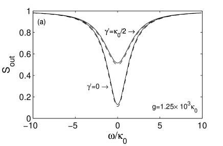
Figure 3: Squeezing spectrum of the field at the cavity output, when the atoms are in a $\lambda/2$-pattern. The dashed lines correspond to the spectrum evaluated analytically from Eq. (30), the solid lines to the spectrum found from the numerical evaluation of the steady state of Eq. (7), see App. A. The frequency is in units of $\kappa_{0}=\kappa$. The parameters are $\Delta=-1.25\times 10^{5}\kappa_{0}$, $\Omega=1.25\times 10^{4}\kappa_{0}$, $g=1.25\times 10^{3}\kappa_{0}$ and $\delta_{c}=-24\kappa_{0}$ ($\delta_{c}$ is chosen so to compensate all a.c.-Stark shifts). For the choice of these parameters, $\alpha=\kappa/2$. The lower and upper curves have been evaluated for $\gamma=0$ and $\gamma^{\prime}=\kappa_{0}/2$ ($\gamma=10^{4}\kappa_{0}$), respectively.

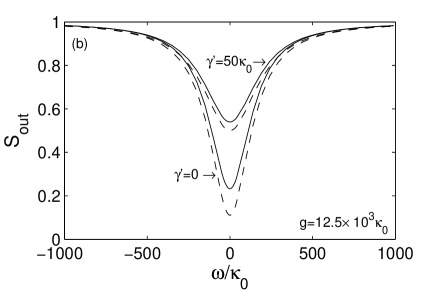
Figure 4: Same as in Fig. 3, where now $\kappa=100\kappa_{0}$, $g=1.25\times 10^{4}\kappa_{0}$, and $\delta_{c}=-24\times 10^{2}\kappa_{0}$. For the choice of these parameters, $\alpha=\kappa/2$. The discrepancy between analytical and numerical results is due to the contribution of the Kerr-nonlinearity, which is not accounted for in the analytical model.

Figure 5 displays the value of the squeezing spectrum at $\omega=0$ as a function of the cavity decay rate $\kappa$. The spectrum is plotted for $\kappa>\alpha$, when the analytical model described by Eqs. (III.2) allows for a steady state solution, and it clearly shows that squeezing at the cavity output is very sensitive to variations of $\kappa$. On the other hand, the dependence on the atomic linewidth $\gamma$ is comparatively weak, as one can see from Fig. 6. The discrepancy between numerical and analytical model at lower values of $\gamma$ is due to the contribution of incoherent scattering processes at higher order, which are accounted for in the numerics and give rise to a very narrow peak at $\omega=0$ in $S(\omega)$. This feature however does not appear for shorter integration times, corresponding to the limit of validity of our perturbative treatment.

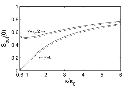
Figure 5: Value of the squeezing spectrum $S_{\rm out}(\omega)$ at $\omega=0$, $S_{\rm out}(0)$, as a function of the cavity decay rate $\kappa$ in units of $\kappa_{0}$. The dashed lines correspond to the value predicted from Eq. (30), the solid lines to the numerical result found from Eq. (7). The parameters are $g=1.25\times 10^{3}\kappa_{0}$, $\Delta=-1.25\times 10^{5}\kappa_{0}$, $\Omega=1.25\times 10^{4}\kappa_{0}$, and $\delta_{c}=-24\kappa_{0}$. For these parameters $\alpha=\kappa_{0}/2$. The lower and upper curves have been evaluated for $\gamma=0$ and $\gamma^{\prime}=\kappa_{0}/2$ ($\gamma=10^{4}\kappa_{0}$), respectively.

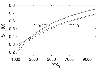
Figure 6: $S_{\rm out}(0)$ as a function of the atomic spontaneous emission rate $\gamma$ in units of $\kappa_{0}$. The spectra are plotted for two values of the cavity decay rate $\kappa=\kappa_{0}$ and $\kappa=\kappa_{0}/2$. The other parameters are as in Fig. 5.

Figures 7(a) and (b) display the spectrum of squeezing at $\omega=0$ and the corresponding variance of the maximally squeezed quadrature of the cavity field as a functions of $\kappa^{\prime}=\kappa+\gamma^{\prime}$. In Fig. 7(a) the upper curves are obtained for $\kappa=\gamma^{\prime}=\kappa^{\prime}/2$, the lower curves correspond to $\gamma^{\prime}=0$, $\kappa^{\prime}=\kappa$. Figure 7(b) shows that the variance of the quadrature is the same both for $\gamma^{\prime}=0$ and $\gamma^{\prime}=\kappa$, showing that spontaneous emission in this regime only dissipates the squeezed field along other channels, as predicted from the analytical model of Eq. (III.2).

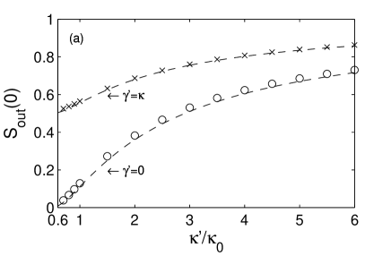
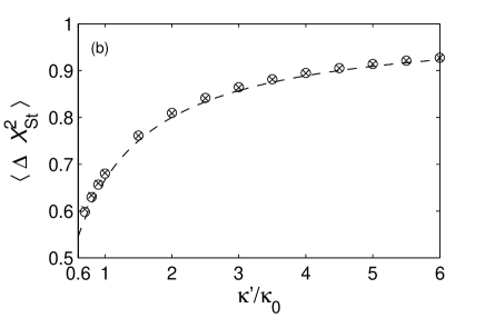
Figure 7: (a) $S_{\rm out}(0)$ as a function of the total effective dissipation rate $\kappa^{\prime}=\kappa+\gamma^{\prime}$ in unit of $\kappa_{0}$ and (b) corresponding variance of the squeezed quadrature of the cavity field. The numerical results are displayed for $\kappa=\kappa^{\prime}$, $\gamma=0$ (circles) and $\kappa=\gamma^{\prime}=\kappa^{\prime}/2$ (crosses). The dashed lines are obtained from the analytical model. The other parameters are $g=1.25\times 10^{3}\kappa_{0}$, $\delta_{c}=-24\kappa_{0}$, $\Delta=-1.25\times 10^{5}\kappa_{0}$, $\Omega=1.25\times 10^{4}\kappa_{0}$, and $\alpha=\kappa_{0}/2$.

IV Effect of the atomic motion

So far we have studied the dynamics of the cavity mode neglecting the atomic kinetic energy on the cavity-mode dynamics. In this section we study the effect of fluctuations in the atomic positions, when the system operates as an optical parameteric amplifier. We assume that the atoms are confined by an external potential, which localize them at the antinodes of the cavity standing wave in a $\lambda/2$-spaced pattern, in the regime in which the mechanical effects of the cavity field on the atomic motion can be neglected. This situation could be realized experimentally with the technology developed for instance in Guthohrlein ; Rauschenbeutel ; Kuhn05 ; Chapman07 .

Denoting by $\bar{x}_{j}$ the atomic equilibrium positions, and by $q_{j}=x_{j}-\bar{x}_{j}$ the displacements, we write the external potential for small vibrations as

$$V(x_{1},x_{2})=\frac{1}{2}M\nu^{2}\left(q_{1}^{2}+q_{2}^{2}\right).$$ (31)

where $\nu$ is the trapping frequency. The Heisenberg-Langevin equation of motion for the atomic displacement $q_{j}$ is given by HelmutFP

$$\ddot{q}_{j}=-\nu^{2}q_{j}-\frac{F^{(j)}}{M}+\xi(t)$$ (32)

where $\xi(t)$ is the quantum Langevin force, associated with the spontaneous emission and the cavity decay processes, and

$${F}^{(j)}=\frac{\partial}{\partial x_{j}}H_{at-cav}$$ (33)

is the mechanical force operator arising from the spatial gradient of the atom-cavity interaction over the atomic wave packet. These equations have to be solved together with the Heisenberg-Langevin equations for the field, which depend on the atomic motion through the functions $\cos kx_{j}$. We assume that the atoms are well localized at the antinodes of the cavity mode, namely that $\delta q=\sqrt{\left\langle q_{j}^{2}\right\rangle}\ll\lambda$, and make a perturbative expansion in the small parameter $k\delta q$. At second order, the equations for the fields read

$$\dot{a}(t) = -{\rm i}\alpha a^{{\dagger}}(t)-\left[\kappa^{\prime}+{\rm i}\left(\theta-\delta_{c}\right)\right]a(t)+\eta\left(t\right)$$

$$+{\rm i}\frac{k^{2}}{2}\left[\left(q_{1}^{2}+q_{2}^{2}\right)\left(\alpha a^{\dagger}(t)+\theta a(t)\right)+\left(q_{1}^{2}-q_{2}^{2}\right)\beta\right]$$

$$\dot{a^{\dagger}}(t) = {\rm i}\alpha a(t)-\left[\kappa^{\prime}-{\rm i}\left(\theta-\delta_{c}\right)\right]a^{\dagger}(t)+\eta\left(t\right)$$

$$-{\rm i}\frac{k^{2}}{2}\left[\left(q_{1}^{2}+q_{2}^{2}\right)\left(\alpha a(t)+\theta a^{\dagger}(t)\right)+\left(q_{1}^{2}-q_{2}^{2}\right)\beta\right]$$

with $\alpha$ defined in Eqs. (21), $\beta=g\Omega/\Delta$, $\theta=2g^{2}\Delta$, and $\eta(t)$ is the quantum Langevin term, $\eta(t)=\sqrt{2\kappa}a_{\rm in}(t)+\sqrt{2\gamma^{\prime}}a^{\rm at}_{\rm in}(t)$. Here $a^{\rm at}_{\rm in}(t)$ is the input noise term associated with atomic spontaneous emission, which satisfy the relation $\left\langle a^{\rm at}_{\rm in}(t){a^{\rm at}_{\rm in}}^{\dagger}(t^{\prime})\right\rangle=\delta(t-t^{\prime})$.

Even when the atoms are well localized around the antinodes of the cavity mode, the systematic solution of these coupled equations is rather complex. Here, we assume that the external potential provides a steep confinement, such that the effect of the coupling with the cavity mode can be neglected in Eq. (32). In this limit the solution of Eq. (32) reads

$$q_{j}(t)\simeq q_{j}^{(0)}\cos(\nu t+\phi_{j}),$$ (36)

where $q_{j}^{(0)}$ and $\phi_{j}$ are determined by the initial conditions. When the trap frequency is much larger than the effective rates which determine the evolution of the field, $\nu\gg\alpha,\kappa^{\prime}$, we can derive a secular equation for the cavity field by averaging the equations for the cavity variables over a period $T=2\pi/\nu$ Blumel . We insert Eq. (36) into the equations for the field variables, Eq. (IV)-(IV), and integrate them over the period $T$. With this procedure we find equations for the operators $\tilde{a}(t)$, $\tilde{\eta}(t)$, defined as

$$\tilde{a}(t)=\frac{1}{T}\int_{t}^{t+T}d\tau a(\tau),~{}~{}\tilde{\eta}(t)=\frac{1}{T}\int_{t}^{t+T}d\tau\eta(\tau)$$ (37)

Here, the new noise operators satisfy the equation $\left\langle\tilde{\eta}(t)\tilde{\eta}^{\dagger}(t^{\prime})\right\rangle\simeq 2\kappa^{\prime}\delta(t-t^{\prime})$, where the $\delta$-like correlation is to be interpreted for the coarse-grained time scale. The corresponding Heisenberg-Langevin equations read

$$\dot{\tilde{a}}(t) = -{\rm i}\tilde{\alpha}\tilde{a}^{\dagger}(t)-\left[\kappa+{\rm i}\left(\tilde{\theta}-\delta_{c}\right)\right]\tilde{a}(t)+\tilde{\eta}(t)$$ (38)

$$\dot{\tilde{a}}(t)^{\dagger} = {\rm i}\tilde{\alpha}\tilde{a}(t)-\left[\kappa-{\rm i}\left(\tilde{\theta}-\delta_{c}\right)\right]\tilde{a}^{\dagger}(t)+\tilde{\eta}^{\dagger}(t)$$ (39)

while their derivation is discussed in App. B. Here,

$$\tilde{\alpha} = \alpha(1-k^{2}\bar{q}^{2}/2)$$

$$\tilde{\theta} = \theta(1-k^{2}\bar{q}^{2}/2).$$ (40)

and we have assumed that the oscillation amplitudes of the two atoms are equal, $q_{1}^{(0)}=q_{2}^{(0)}=\bar{q}$. The motion-induced a.c.-Stark shift can be compensated by properly tuning the laser frequency, $\tilde{\delta}_{c}=\theta(1-k^{2}\bar{q}^{2}/2)$, and Eqs. (38)-(39) become

$$\dot{\tilde{a}}(t) = -{\rm i}\tilde{\alpha}\tilde{a}^{\dagger}(t)-\kappa^{\prime}\tilde{a}(t)+\tilde{\eta}(t)$$

$$\dot{\tilde{a}}(t) = {\rm i}\tilde{\alpha}\tilde{a}(t)-\kappa^{\prime}\tilde{a}^{\dagger}(t)+\tilde{\eta}^{\dagger}(t).$$ (41)

Correspondingly, at lowest order in $k\bar{q}_{j}$ the spectrum of squeezing is

$$S_{\rm out}(\omega) = 1-\frac{4\kappa\alpha}{\left(\kappa^{\prime}+\alpha\right)^{2}+\omega^{2}}$$ (42)

$$\times\left[1+\frac{\left(\alpha^{2}-{\kappa^{\prime}}^{2}-\omega^{2}\right)}{\left(\kappa^{\prime}+\alpha\right)^{2}+\omega^{2}}\frac{k^{2}\bar{q}^{2}}{2}\right]$$

where the term proportional to $k^{2}\bar{q}^{2}$ is the correction to Eq. (30) due to small vibrations of the atoms at the equilibrium positions. Small fluctuations hence reduce the bandwidth of frequencies where the light is squeezed. The corresponding spectrum, Eq. (42), is displayed in Fig. 8 for $k\bar{q}=0.3$ and compared to the one of Eq. (30), where atomic motion is neglected, showing that the modification of the spectrum of squeezing due to the motion is very small.

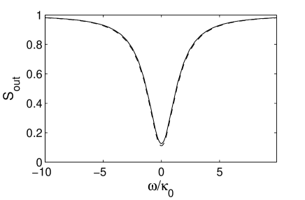
Figure 8: Spectrum of squeezing of the field at the cavity output as a function of $\omega$ in units of $\kappa_{0}$, for the same parameters as in Fig. 3 and $\gamma=0$. The solid curve corresponds to the spectrum of Eq. (IV) for $k\bar{q}=0.3$. The dashed line corresponds to the spectrum of Eq. (30) when atomic vibrations are neglected.

V Conclusion

We have studied the dynamics and steady state of a medium composed by two atomic dipoles confined inside a resonator in an ordered structure. Depending on the relative position of the atoms inside the cavity mode, the linear response can be suppressed, and by tuning the intensity of the laser the system can operate as Kerr medium or as optical parametric amplifier, whereby the nonlinear response emerges from the collective excitations of the atomic dipoles. We have studied in detail the case in which the system operates as an optical parametric amplifier, and investigated the squeezing of the field at the cavity output considering the effects of atomic vibrations, when the atoms are confined inside the resonator at the equilibrium positions of a steep external potential, in a situation which can be experimentally realized for instance in Guthohrlein ; Rauschenbeutel ; Kuhn05 ; Chapman07 .

A natural question, emerging from recent studies on selforganization of laser-cooled atoms in resonators Domokos02 ; Asboth05 ; Chan03 ; Black03 , is whether in absence of an external potential trapping the atoms, the $\lambda/2$-spaced pattern can be sustained by the mechanical forces of the potential generated by the scattered field. In Asboth04 a semiclassical and numerical analysis showed that this configuration is expected to be stable for choices of the parameters, which are consistent with the operational regime in which squeezed light can be observed. In this case, one would hence have a selforganized pattern, which sustains and is sustained by non-classical light.

The results of this work provide an example of how non-linearities emerge from the microscopic dynamics of few simple quantum systems. In this respect, two atoms in a resonator can be considered the most basic realization of a non-linear crystal, with however limited efficiencies. We conjecture that by scaling up the number of atoms collective effects can enhance the nonlinear properties, thus improving the system response. Another interesting question is how the system dynamics are modified when the quantum nature of the atomic motion is relevant Maschler06 ; Larson07 , and in particular how the correlation functions of the output field are affected by the quantum properties of the medium. This study requires an analysis of the spectrum of resonance fluorescence as in Zippilli07 , which systematically accounts for the quantum state of the atomic motion, and it will be object of future investigations.

Appendix A Evaluation of the Squeezing spectrum

Using Eq (29), we rewrite the squeezing spectrum in Eq. (27) as

$$S_{\rm out}(\omega)=1+4\kappa{\rm Re}\int_{0}^{\infty}dt{\rm e}^{-{\rm i}\omega t}\left[\langle a(t),a(0)\rangle_{\rm St}{\rm e}^{-2{\rm i}\pi/4}\right.$$

$$\left.+\langle a^{\dagger}(0),a^{\dagger}(t)\rangle_{\rm St}{\rm e}^{2{\rm i}\pi/4}+\langle a^{\dagger}(t),{a(0)}\rangle_{\rm St}+\langle a^{\dagger}(0),a(t)\rangle_{\rm St}\right].$$

where

$$\langle a^{\dagger}(0),a^{\dagger}(t)\rangle_{\rm St}=\langle a^{\dagger}(0)a^{\dagger}(t)\rangle_{\rm St}-\langle a^{\dagger}(0)\rangle_{\rm St}\langle a^{\dagger}(t)\rangle_{\rm St}.$$

Equation (A) can be expressed in terms of averages performed over a density matrix by means of the relation $\left\langle A(t)A(0)\right\rangle_{\rm St}={\rm Tr}\left\{A{\rm e}^{{\cal L}t}A\rho_{\rm St}\right\}$ and $\left\langle A(0)A(t)\right\rangle_{\rm St}={\rm Tr}\left\{A{\rm e}^{{\cal L}t}\rho_{\rm St}A\right\}$, where $A$ is a generic operator, $\cal L$ is the Liouvillian defined in Eq. (8) setting $H_{mec}=0$, and $\rho_{\rm St}$ is the steady state density matrix satisfying the relation ${\cal L}\rho_{\rm St}=0$. Therefore the spectrum of squeezing can be rewritten as

$$S^{(\theta)}_{\rm out}(\omega)=1-4\kappa{\rm Re}\left[\pi\delta\left(\omega\right){\rm Tr}\left\{X^{(\theta)}\rho_{\rm St}\right\}^{2}\right.$$

$$+\left.{\rm Tr}\left\{X^{(\theta)}\left({\cal L}-{\rm i}\omega\right)^{-1}\left(a\rho_{\rm St}{\rm e}^{-{\rm i}\theta}+\rho_{\rm St}a^{\dagger}{\rm e}^{{\rm i}\theta}\right)\right\}\right]$$ (44)

The numerical results in Sec. III.3 are based on the evaluation of the spectrum of squeezing, as calculated from Eq. (A) using the Liouvillian of Eq.( 7).

Appendix B Derivation of the secular equations for fast vibrating atoms

After inserting Eq. (36) into the Eqs. Eqs. (IV)-(IV), we obtain

$$\dot{A}(t) = MA(t)+N(t)$$

$$+\sum_{j=1,2}k^{2}\bar{q}_{j}^{2}\cos^{2}(\nu t+\phi_{j})\left[VA(t)+(-1)^{j}B\right]$$

where

$$A(t)=\left(\begin{array}[]{c}a(t)\\ a^{\dagger}(t)\end{array}\right),$$ (48)

$$M=\left(\begin{array}[]{cc}-\kappa^{\prime}-{\rm i}(\theta-\delta_{c})&-{\rm i}\alpha\\ {\rm i}\alpha&-\kappa^{\prime}+{\rm i}(\theta-\delta_{c})\end{array}\right),$$ (51)

$$N(t)=\left(\begin{array}[]{c}\eta(t)\\ \eta^{\dagger}(t)\end{array}\right),$$ (54)

$$V=\left(\begin{array}[]{cc}{\rm i}\theta/2&{\rm i}\alpha/2\\ -{\rm i}\alpha/2&-{\rm i}\theta/2\end{array}\right),$$ (57)

and

$$B=\left(\begin{array}[]{c}-{\rm i}\beta\\ {\rm i}\beta\end{array}\right).$$ (60)

We indicate with

$$\tilde{f}(t)=\frac{1}{T}\int_{t}^{t+T}d\tau f(\tau)$$ (61)

the time average of a variable $f(t)$ over a period of oscillation $T=2\pi/\nu$ of the atomic motion. Since

$$\frac{\partial}{\partial t}\tilde{f}(t)=\frac{1}{T}\left[f(t+T)-f(t)\right]=\widetilde{\frac{\partial f}{\partial t}},$$

we find

$$\frac{\partial}{\partial t}\tilde{A}(t) = M\tilde{A}(t)+\tilde{N}(t)+k^{2}\bar{q}^{2}V\tilde{A}(t)$$

$$+k^{2}\bar{q}^{2}\frac{V}{2}\sum_{j=1,2}\frac{1}{T}\int_{t}^{t+T}d\tau{\cos(2\nu\tau+2\phi_{j})A(\tau)}$$

where we have used the relation $\cos^{2}(y)=\frac{1}{2}\left[1+\cos(2y)\right]$ and we have assumed that the two atoms have the same energy, such that $\bar{q}_{1}^{2}=\bar{q}_{2}^{2}=\bar{q}^{2}$. We now identify the conditions under which we can neglect the second line of Eq. (B). Integrating by part the second line of Eq. (B) an using Eqs. (B) and (B) we obtain

$$\frac{\partial}{\partial t}\tilde{A}(t) = M\tilde{A}(t)+\tilde{N}(t)+k^{2}\bar{q}^{2}V\tilde{A}(t)$$ (63)

$$+k^{2}\bar{q}^{2}C(t)+k^{4}\bar{q}^{4}D(t)+k^{4}\bar{q}^{4}E$$

where

$$C(t) = \frac{V}{4\nu}\sum_{j}\left\{\sin(2\nu t+2\phi_{j})\left[M\tilde{A}(t)+\tilde{N}(t)\right]\right.$$

$$\left.-\frac{1}{T}\int_{t}^{t+T}d\tau\sin(2\nu\tau+2\phi_{j})\left[M{A}(\tau)+{N}(\tau)\right]\right\},$$

$$D(t) = \frac{V^{2}}{8\nu T}\sum_{jj^{\prime}}\int_{t}^{t+T}d\tau$$

$$\times\left[\sin(2\nu t+2\phi_{j})\right.\cos(2\nu\tau+2\phi_{j^{\prime}})$$

$$\left.-2\sin(2\nu\tau+2\phi_{j})\cos^{2}(\nu\tau+\phi_{j^{\prime}})\right]A(\tau),$$

$$E = \frac{VB}{8\nu}\sin[2(\phi_{2}-\phi_{1})].$$ (64)

The terms $k^{2}\bar{q}^{2}C(t)+k^{4}\bar{q}^{4}D(t)$ are negligible with respect to $k^{2}\bar{q}^{2}V$ when $\left|{\theta}\right|\kappa^{\prime}/8\nu\ll\left|{\alpha}\right|/2$ and $\left|{\theta(\theta-\delta_{c})}\right|/8\nu\ll\left|{\alpha}\right|/2$ which reduce to

$$\nu \gg \frac{g^{2}}{\left|{\Delta}\right|},$$ (65)

$$\nu \gg \frac{k^{2}\bar{q}^{2}}{8}\left|{\frac{g^{2}\Delta}{\Omega^{2}}}\right|$$ (66)

when $|\alpha|$ and $\kappa^{\prime}$ are of the same order of magnitude and $\delta_{c}=\theta(1-k^{2}\bar{q}^{2}/2)$, see Eq. (40). The term $k^{4}\bar{q}^{4}E$ in Eq. (63) can be neglected when $k^{4}\bar{q}^{4}\left|{\theta\beta}\right|/16\nu\ll k^{2}\bar{q}^{2}\left|{\alpha}\right|/2$, that is

$$\nu \gg \frac{k^{2}\bar{q}^{2}}{16}\left|{\frac{g\Delta}{\Omega}}\right|.$$ (67)

When conditions (65)-(67) are satisfied we approximate Eq. (B) with

$$\frac{\partial}{\partial t}\tilde{A}(t) = M\tilde{A}(t)+\tilde{N}(t)+k^{2}\bar{q}^{2}V\tilde{A}(t).$$

which then leads to Eqs. (38) and (39). Finally we show that the averaged noise operators, $\tilde{\eta}(t)$ and $\tilde{\eta}^{\dagger}(t)$, which appear in the term $\tilde{N}(t)$, are delta correlated. The only non-vanishing correlation function is

$$\left\langle\tilde{\eta}(t)\tilde{\eta}^{\dagger}(t^{\prime})\right\rangle=\frac{2\kappa^{\prime}}{T^{2}}\int_{t}^{t+T}d\tau\int_{t^{\prime}}^{t^{\prime}+T}d\tau^{\prime}\delta\left(\tau-\tau^{\prime}\right)$$

$$=\left\{\begin{array}[]{l}\frac{2\kappa^{\prime}}{T^{2}}\left(t^{\prime}+T-t\right)\ {\rm for}\ t^{\prime}<t<t^{\prime}+T\\ \frac{2\kappa^{\prime}}{T^{2}}\left(t+T-t^{\prime}\right)\ {\rm for}\ t^{\prime}-T<t<t^{\prime}\\ 0\ \ \ \ \ {\rm for}\ t>t^{\prime}+T\ {\rm or}\ t<t^{\prime}-T\end{array}\right.$$ (72)

which is not zero only if the two integration intervals $[t,t+T]$ and $[t^{\prime},t^{\prime}+T]$ have finite overlap. Therefore if ${f}(t)$ varies slowly over the time $T$, so that $\tilde{f}(t)\simeq f(t)$, then one has

$$\int_{-\infty}^{\infty}dtf(t)\left\langle\tilde{\eta}(t)\tilde{\eta}^{\dagger}(t^{\prime})\right\rangle\simeq 2\kappa^{\prime}f(t^{\prime}),$$ (74)

that is $\left\langle\tilde{\eta}(t)\tilde{\eta}^{\dagger}(t^{\prime})\right\rangle\simeq 2\kappa^{\prime}\delta(t-t^{\prime})$.

References

- (1) P. Zoller et al., Quantum information processing and communication, Eur. Phys. J. D 36, 203 (2005).
- (2) H.J. Briegel, W. Dür, J.I. Cirac, P. Zoller, Phys. Rev. Lett. 81, 5932 (1998).
- (3) B. Kraus and J. I. Cirac, Phys. Rev. Lett. 92, 013602 (2004).
- (4) S.L. Braunstein, P. van Loock, Rev. Mod. Phys. 77, 513 (2005).
- (5) M. Keller, B. Lange, K. Hayasaka, W. Lange, H. Walther, Nature 431, 1075 (2004).
- (6) J. McKeever, A. Boca, A.D. Boozer, J.R. Buck, H.J. Kimble, Nature 425, 268 (2003).
- (7) J. McKeever, A. Boca, A.D. Boozer, R. Miller, J.R. Buck, A. Kuzmich, H.J. Kimble, Science 303, 1992 (2004).
- (8) A. Kuhn, M. Hennrich, G. Rempe, Phys. Rev. Lett. 89, 067901 (2002).
- (9) T. Wilk, S.C. Webster, H.P. Specht, G. Rempe, A. Kuhn, Phys. Rev. Lett. 98, 063601 (2007) .
- (10) M.D. Eisaman, L. Childress, A. André, F. Massou, A.S. Zibrov, M.D. Lukin, Phys. Rev. Lett. 93, 233602 (2004).
- (11) J.S. Neergaard-Nielsen, B.M. Nielsen, C. Hettich, K. Mølmer, E.S. Polzik, Phys. Rev. Lett. 97, 083604 (2006).
- (12) D.N. Matsukevich, T. Chanelière, S.D. Jenkins, S.Y. Lan, T.A. Kennedy, A. Kuzmich, Phys. Rev. Lett. 97, 013601 (2006).
- (13) B. Darquie, M.P.A. Jones, J. Dingjan, J. Beugnon, S. Bergamini, Y. Sortais, G. Messin, A. Browaeys, P. Grangier Science 309, 454 (2005)
- (14) A. Ourjoumtsev, R. Tualle-Brouri, J. Laurat, P. Grangier, Science 312, 83 (2006).
- (15) B. B. Blinov, D. L. Moehring, L. - M. Duan, C. Monroe, Nature 428, 153-157 (2004).
- (16) J. Volz, M. Weber, D. Schlenk, W. Rosenfeld, J. Vrana, K. Saucke, C. Kurtsiefer, H. Weinfurter, Phys. Rev. Lett. 96, 030404 (2006).
- (17) T. Savels, A.P. Mosk, and A. Lagendijk, Phys. Rev. Lett. 98, 103601 (2007).
- (18) D.F. Walls and G.J. Milburn, Quantum optics (Springer, Berlin, 1994).
- (19) J. A. Armstrong, N. Bloembergen, J. Ducuing, P. S. Pershan, Phys. Rev. 127, 1918-1939 (1962).
- (20) R. W. Boyd, Nonlinear Optics (Academic Press, Inc., London, 1992).
- (21) A. Imamoglu, H. Schmidt, G. Woods, and M. Deutsch, Phys. Rev. Lett. 79, 1467 (1997). See also Ph. Grangier, D.F. Walls, and K.M. Gheri, Phys. Rev. Lett. 81, 2833 (1998); A. Imamoglu, H. Schmidt, G. Woods, M. Deutsch, Phys. Rev. Lett. 81, 2836 (1998).
- (22) A. S. Parkins and H. J. Kimble, J. Opt. B: Quantum Semiclass. Opt. 1, 496 (1999).
- (23) G. Morigi, J. Eschner, S. Mancini, D. Vitali, Phys. Rev. Lett. 96, 023601 (2006); G. Morigi, J. Eschner, S. Mancini, and D. Vitali, Phys. Rev. A 73, 033822 (2006).
- (24) D. Vitali, G. Morigi, and J. Eschner, Phys. Rev. A 74, 053814 (2006).
- (25) S. Zippilli and G. Morigi, Phys. Rev. A 72, 053408 (2005).
- (26) S. Zippilli, G. Morigi, H. Ritsch, Phys. Rev. Lett. 93, 123002 (2004); S. Zippilli, G. Morigi, H. Ritsch, Eur. Phys. J. D 31, 507 (2004).
- (27) P.M. Alsing, D.A. Cardimona, H.J. Carmichael, Phys. Rev. A 45, 1793 (1992).
- (28) W. Vogel and D.-G. Welsch, Phys. Rev. Lett. 54, 1802 (1985).
- (29) P. Domokos, H. Ritsch, Phys. Rev. Lett. 89, 253003 (2002).
- (30) J.K. Asbóth, P. Domokos, H. Ritsch, A. Vukics, Phys. Rev. A 72, 053417 (2005).
- (31) H.W. Chan, A.T. Black, V. Vuletic, Phys. Rev. Lett. 90, 097902 (2003).
- (32) A.T. Black, H.W. Chan, V. Vuletic, Phys. Rev. Lett. 91, 203001 (2003).
- (33) S. Zippilli, J. Asbóth, G. Morigi, H. Ritsch, Appl. Phys. B: Lasers Opt. 79, 969 (2004).
- (34) G. R. Guthohrlein, M. Keller, K. Hayasaka, W. Lange, H. Walther, Nature 414, 49-51 (2001).
- (35) S. Nu mann, M. Hijlkema, B. Weber, F. Rohde, G. Rempe, A. Kuhn, Phys. Rev. Lett. 95, 173602 (2005).
- (36) I. Dotsenko, W. Alt, M. Khudaverdyan, S. Kuhr, D. Meschede, Y. Miroshnychenko, D. Schrader, A. Rauschenbeutel, Phys. Rev. Lett. 95, 033002 (2005).
- (37) K.M. Fortier, S.Y. Kim, M.J. Gibbons, P. Ahmadi, M.S. Chapman, Phys. Rev. Lett. 98, 233601 (2007)
- (38) P. Domokos, P. Horak, H. Ritsch, J. Phys. B: At. Mol. Opt. Phys. 34, 187 198 (2001).
- (39) See for instance, R. Blumel, Phys. Rev. A 51, 620 (1995).
- (40) C. Maschler, H. Ritsch , Phys. Rev. Lett. 95, 260401 (2005).
- (41) J. Larson, B. Damski, G. Morigi, M. Lewenstein, cond-mat/0608335.
- (42) M. Bienert, J. M. Torres, S. Zippilli, G. Morigi, Phys. Rev. A 76, 013410 (2007).