The statistical properties of $\Lambda$CDM halo formation

Abstract

We present a comparison of the statistical properties of dark matter halo merger trees extracted from the Millennium Simulation with Extended Press-Schechter (EPS) formalism and the related GALFORM Monte-Carlo method for generating ensembles of merger trees. The volume, mass resolution and output frequency make the Millennium Simulation a unique resource for the study of the hierarchical growth of structure. We construct the merger trees of present day friends-of-friends groups and calculate a variety of statistics that quantify the masses of their progenitors as a function of redshift; accretion rates; and the redshift distribution of their most recent major merger. We also look in the forward direction and quantify the present day mass distribution of halos into which high redshift progenitors of a specific mass become incorporated. We find that EPS formalism and its Monte-Carlo extension capture the qualitative behaviour of all these statistics but, as redshift increases they systematically underestimate the masses of the most massive progenitors. This shortcoming is worst for the Monte-Carlo algorithm. We present a fitting function to a scaled version of the progenitor mass distribution and show how it can be used to make more accurate predictions of both progenitor and final halo mass distributions.

1 Introduction

The $\Lambda$CDM cosmological model is specified by a small number of parameters most of which are accurately constrained by a combination of data from the cosmic microwave background and large-scale structure (Sánchez et al., 2006; Spergel et al., 2007). Thus, the initial conditions for the formation of structure are well determined and the subsequent hierarchical growth of structure, involving the formation and merging of dark matter halos, can be simulated with considerable rigour using large cosmological N-body simulations. However, because of their computational expense or in order to extrapolate to different parameter values, frequent use is made of approximate analytic and Monte-Carlo descriptions of halo formation and halo mergers.

In this paper, we extract statistical properties of the merger histories of dark matter halos in the Millennium Simulation (MS, Springel et al., 2005a) and compare them to Extended Press-Schechter (EPS) formalism (Bond et al., 1991; Bower, 1991; Lacey & Cole, 1993, 1994) and to the Monte-Carlo algorithm for generating dark matter halo merger trees that is incorporated in the GALFORM semi-analytic model of galaxy formation (Cole et al., 2000; Benson et al., 2003; Baugh et al., 2005). In this way one can determine the strengths and weaknesses of the current descriptions and provide the information required to test future improvements to such models.

The merger history of a dark matter halo is perhaps best visualised as a merger tree (e.g. see the schematic figure 6 in Lacey & Cole, 1993) in which small halos present at some early redshift $z$ come together through a series of merger events to form a single halo by redshift $z=0$. The most widely used statistical description of these merger trees is the EPS formalism introduced by Bond et al. (1991) and Bower (1991) and developed by Lacey & Cole (1993). For a given set of cosmological model parameters, this analytic model predicts the ensemble average properties of sets of merger trees as a function of the final halo mass. Thus, for instance, one can take a galaxy cluster of mass $10^{15}$ M_⊙ today and ask, on average, how many of its progenitor halos (the halos that merged to form it) at redshift $z=1$ had masses greater than $10^{14}$ M_⊙. However, EPS formalism alone will not yield any information about the distribution around this mean, such as how often there are $5$ such progenitors. To build algorithms capable of generating sets of individual merger trees and so be able to make predictions for any such statistics requires further assumptions. This has been done in various ways (Cole, 1991; Kauffmann & White, 1993; Sheth & Pitman, 1997; Sheth & Lemson, 1999; Somerville & Kolatt, 1999; Cole et al., 2000). It is important to test these algorithms and not just the EPS formalism as many interesting observational questions, such as what fraction of galaxy halos undergo major mergers in the last $2$ Gyr, depend not on the mean of the distribution, but on the properties of the tails. Thus, here we not only update the tests of the EPS formalism made in Lacey & Cole (1994), but also look at various statistics that test the progenitor distributions predicted by the Monte-Carlo algorithm often used in the GALFORM semi-analytic code (Cole et al., 2000).

In Section 2 we briefly describe the properties of the MS and how we identify halos and build merger trees. The theoretical models to which we compare our results are reviewed in Section 3. Section 4 presents a series of statistical measures of the merger histories, comparing each to the model predictions and includes, in Section 4.1, the examination of a new empirical model for the conditional mass function. We conclude in Section 5.

2 The Millennium Simulation

The Millennium Simulation follows the gravitational evolution of $N=2160^{3}$ particles in a comoving periodic cube of side $L=500h^{-1}$ Mpc. The initial conditions are a Gaussian random field with a power spectrum consistent with the combined analysis of the 2dFGRS (Percival et al., 2001) and first year WMAP data (Spergel et al., 2003). Specifically, the total matter, baryon and cosmological constant density parameters are $\Omega_{\rm m}=0.25$, $\Omega_{\rm b}=0.045$ and $\Omega_{\Lambda}=0.75$, respectively; the slope of the primordial power spectrum is $n=1$; the Hubble parameter $h\equiv H_{0}/100\,{\rm km\,s^{-1}\,Mpc^{-1}}=0.73$; and the amplitude of the density fluctuations, expressed as the linear rms mass fluctuation in spheres of radius $8\,h^{-1}$ Mpc at $z=0$, is $\sigma_{8}=0.9$. The resulting particle mass in the simulation is $8.6\times 10^{8}h^{-1}$ M_⊙ and the force softening (Plummer equivalent) is $\epsilon=5h^{-1}$ kpc. The simulation was performed with a special, memory efficient version of the GADGET-2 code (Springel, 2005b). Further details of the MS can be found in Springel et al. (2005a).

The MS produced outputs, including catalogues of friends-of-friends (FOF, Davis et al., 1985)) groups of $20$ or more particles defined using a linking length parameter $b=0.2$, at approximately $60$ redshifts. The substructure within each of these groups was quantified using the SUBFIND algorithm (Springel et al., 2001) which identifies self-bound overdensities within each group. To follow halo formation one must follow the descendants of each halo from one timestep to the next. Linking MS halos together in this way to form merger trees has been done in a variety of different ways. The merger trees used in the semi-analytic models of the Munich group (Springel et al., 2005a; Croton et al., 2006; De Lucia et al., 2006) use as their basic unit the sub-halos found by SUBFIND and link these between timesteps. In contrast, the merger trees used by the Durham group (Bower et al., 2006) primarily link FOF groups between timesteps, but make use of the SUBFIND information both to split FOF groups that become prematurely or temporarily linked by low density bridges (for a description of how this is done see Harker et al., 2006) and to follow the location of galaxies within the halos.

Here, we have decided to analyse merger trees based solely on linking FOF groups. For each FOF group at one timestep, we trace the most bound 10% of the particles (or the ten most bound particles, if 10% would be fewer than ten particles) in the most massive subhalo and adopt as the descendant at the next timestep the halo that contains the largest number of these particles. Normally, the vast majority are in the same halo. This choice has the virtue of being simple and easily reproducible. Also, the occasional splitting of halos performed in the more complicated merger trees used in Bower et al. (2006), while important for the formation of individual halos and galaxies, has very little effect on most of the statistical quantities we present in this paper. We have, in fact, also analysed the merger trees used in Bower et al. (2006) and, wherever there is a significant difference, we comment appropriately.

3 Models

The original Press & Schechter (1974) theory was just a model for the mass function,

$$f(M)\,d\ln M=\sqrt{\frac{2}{\pi}}\frac{\delta}{\sigma}\ \exp\left[-\frac{1}{2}\frac{\delta^{2}}{\sigma^{2}}\right]\left|\frac{d\ln\sigma}{d\ln M}\right|\,d\ln M,$$ (1)

of halos as a function of redshift. Here, $f(M)$ is the fraction of mass in halos of mass $M$; $\delta(z)$ is the linear density threshold for spherical collapse at redshift $z$; and $\sigma(M)$ is the rms amplitude of linear density fluctuations when smoothed on a mass scale $M$. For comparison with the MS we adopt $\delta(z)$ for a $\Lambda$CDM cosmology as calculated by Eke et al. (1996) and $\sigma(M)$ computed from the linear power spectrum used to create the MS initial conditions, with a real-space spherical top-hat window window function. If one defines the variable $\nu=\delta/\sigma$, then the Press-Schechter mass function can be written compactly as

$$f(M)\,d\ln M=f_{\rm PS}(\nu)\left|\frac{d\ln\nu}{d\ln M}\right|\,d\ln M,$$ (2)

where

$$f_{\rm PS}(\nu)=\sqrt{\frac{2}{\pi}}\,\nu\,\exp(-\nu^{2}/2).$$ (3)

The alternative derivation of the Press & Schechter model by Bond et al. (1991) using an excursion set approach placed the theory on a firmer footing and also showed how the model could be extended to yield conditional mass functions describing the progenitors of halos of different final masses (see Bower, 1991, for an alternative derivation of this result). The Bond et al. (1991) derivation makes several assumptions. It computes the threshold overdensity for collapse using the pure spherical collapse model; the linear overdensity at a given point in space is assumed to vary with the smoothing scale as an uncorrelated (Brownian) random walk (the sharp $k$-space filtering approximation); when assigning mass points to halos of mass $M$ no condition is set to demand that these mass points should lie in spatially localised regions capable of forming halos of that mass. It is thus no surprise that the model does not exactly match the results of the large non-linear N-body simulations that current technology allows (Jenkins et al., 2001). In fact, it is perhaps surprising that the theory performs as well as it does. This may be because despite the approximations made in deriving the model, it has the scaling properties that make it fully consistent with self-similar evolution (for example, see Efstathiou et al., 1988) and is fully self-consistent.

Sheth et al. (2001) and Sheth & Tormen (2002) showed that by dropping the first assumption described above and modelling the density threshold for collapse using an elliptical model one could modify the Press-Schechter mass function to be in excellent agreement with N-body simulations. This modification considerably complicates the model and, in particular, destroys the symmetry that allows the conditional mass functions to be derived analytically. Also, for small time intervals, Sheth & Tormen (2002) found that their model predicted conditional mass functions which are in worse agreement with the simulation data than the original EPS model. Thus, by completely removing the inaccuracy of the mass function by revising just one of the three simplifying assumptions of the EPS model other aspects of the model are made worse.

Here, because of its simplicity and because it is still the only analytic model that lends itself to the generation of individual merger trees, we compare the MS with the original EPS formalism (Bond et al., 1991; Bower, 1991). The Monte-Carlo algorithm whose merger trees we compare with those of the MS is that described in section 3.1 of Cole et al. (2000). This algorithm is derived by computing, using the EPS formalism, the distribution of progenitors in the limit of an infinitesimally small timestep. This is used to compute both the probability that a halo of mass $M_{\rm final}$ at redshift $z$ splits into two progenitors at time $dz$ earlier and the probability that one of the progenitors has mass $M_{1}$. Implicit in this algorithm is the assumption that the probability of having a progenitor of mass $M_{1}$ should be equal to that of having one of mass $M_{2}=M_{\rm final}-M_{1}$, since the two progenitors must add up to the mass of the final object. However, in general, the progenitor mass distribution given by the EPS theory does not respect this symmetry. In fact, only in the case of Poisson initial conditions ($P(k)=k^{n}$ with $n=0$) is this symmetry reproduced by the EPS theory (e.g. Sheth & Pitman, 1997). Only in this one special case is the tree generating algorithm in Cole et al. (2000) exact and the average properties of the merger trees it produces are in exact agreement with the conditional mass functions produced by the EPS theory . For the case of Poisson initial conditions, algorithms for generating merger trees were first presented by Sheth & Pitman (1997) and Sheth & Lemson (1999), while Sheth (1996) computed analytic expressions for the higher order moments of such trees. For the more relevant cases such as the $\Lambda$CDM model we investigate here, the inconsistency of the Monte-Carlo algorithm with the EPS theory causes the progenitor mass function to evolve with redshift a little more rapidly than it should. We illustrate this below by comparing the conditional mass functions of EPS theory both with the MS results and with those derived from the Monte-Carlo algorithm.

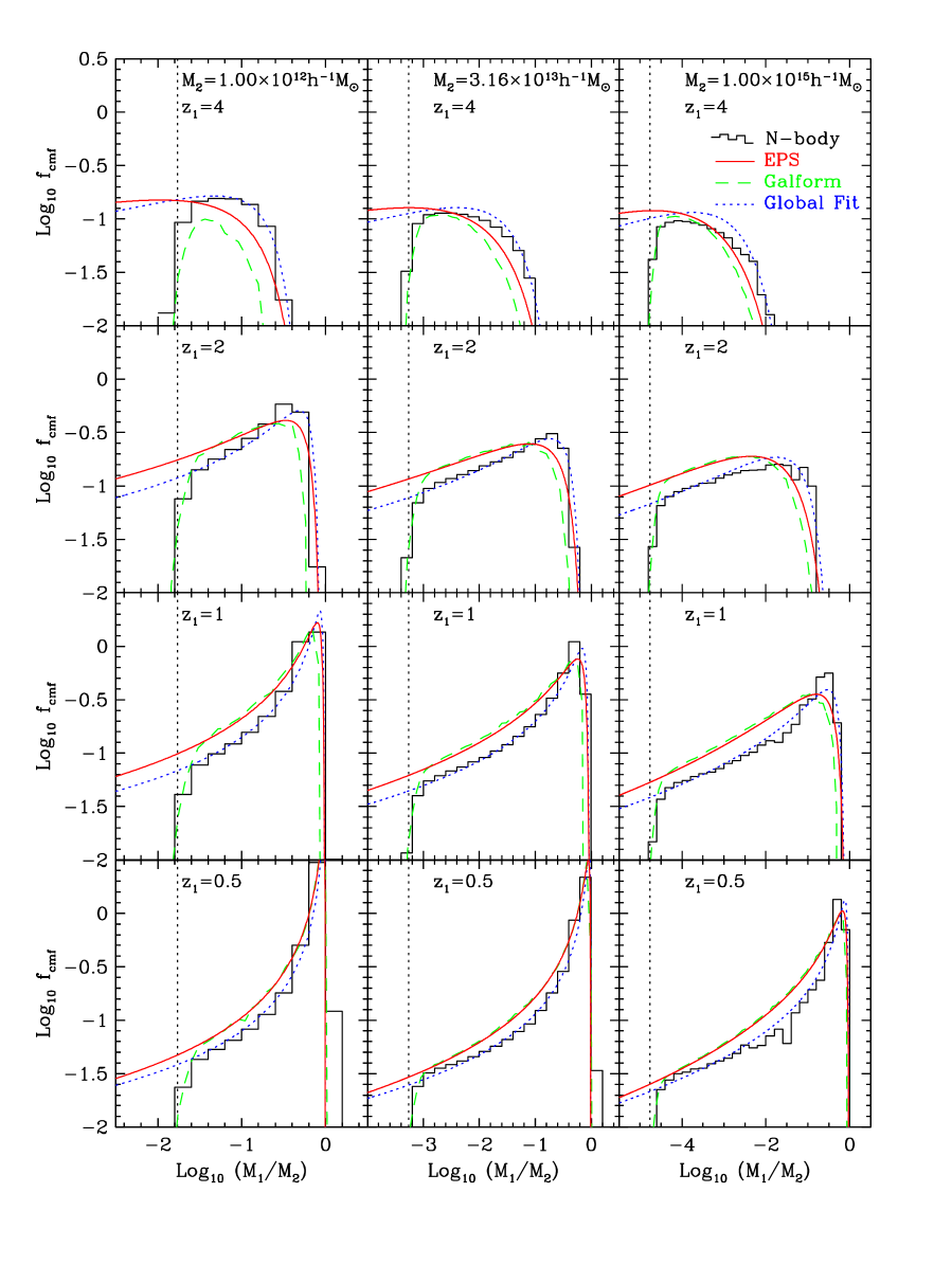
Figure 1: The fraction of mass in progenitor halos of mass $M_{1}$ in bins of $\log_{10}M_{1}/M_{2}$ at redshifts $z=0.5,1,2$ and $4$ as indicated, for three different masses $M_{2}$ (indicated at the top of each column). The histograms show the results from the Millennium Simulation while the solid and dashed curves show the corresponding conditional mass functions given by the EPS formalism and the GALFORM Monte-Carlo algorithm respectively. The dotted curves show the prediction of the Global Fit given in equation (7). The vertical dotted lines indicate the 20 particle mass resolution limit of the Millennium simulation.

4 Results

In the following subsections we look at a variety of statistics that probe complementary aspects of the merger statistics of forming dark matter halos.

4.1 Conditional mass functions of progenitors

Fig. 1 shows the conditional mass functions at redshifts $z=0.5,1,2$ and $4$, for halos which at redshift $z_{2}=0$, have mass $M_{2}=1.0\times 10^{12}$, $3.16\times 10^{13}$ and $1.0\times 10^{15}h^{-1}$ M_⊙. We choose these three mass bins, separated by $\sqrt{1000}$ in mass, to span the dynamic range of the MS. In each bin, we average over halos within a factor of $\sqrt{2}$ of the central mass. In order of increasing mass, this gives samples of $264\,300$, $11\,350$ and  $82$ halos in the three bins. The fraction plotted on the $y$-axis is the fraction of the final halo mass that is in progenitors of mass $M_{1}$ per unit bin in $\log_{10}M_{1}$. Plotted on the $x$-axis is $\log_{10}M_{1}/M_{2}$ which avoids the histograms being smoothed due to the variation in $M_{2}$. The $20$ particle mass resolution limit of the MS is indicated in each panel by the vertical dotted line. The N-body results are truncated below this mass, but this truncation is not completely sharp because of the range of $M_{2}$ used in each sample. In a completely hierarchical model, $M_{1}$ should always be less than $M_{2}$, but there are rare occasions in the MS where a progenitor looses mass. This can occur when two halos are in the process of merging and they are temporarily linked by the FOF algorithm. Most of these cases are identified and removed by the more complicated merger tree building algorithm used with the semi-analytic galaxy formation models, but here, with the simple FOF scheme, they give rise to two populated bins with $M_{1}/M_{2}>1$ at $z=0.5$.

The solid curves show the analytic predictions of the EPS theory,

$$\displaystyle{f(M_{1}|M_{2})\,d\ln M_{1}=\sqrt{\frac{2}{\pi}}\,\frac{\sigma_{1}^{2}(\delta_{1}-\delta_{2})}{[\sigma_{1}^{2}-\sigma_{2}^{2}]^{3/2}}}\,\times$$ (4)

$$\displaystyle{\exp\left[-\frac{1}{2}\frac{(\delta_{1}-\delta_{2})^{2}}{(\sigma_{1}^{2}-\sigma_{2}^{2})}\right]\left|\frac{d\ln\sigma}{d\ln M_{1}}\right|\,d\ln M_{1}},$$

where $\delta_{1}$ is the threshold for collapse at the redshift being considered and $\delta_{2}$ the corresponding threshold at redshift $z=0$. The amplitude of the rms density fluctuations smoothed on scales $M_{1}$ and $M_{2}$ are denoted as $\sigma_{1}$ and $\sigma_{2}$ respectively. In Bond et al. (1991) this formula was derived by a very simple coordinate transformation and can be written neatly as

$$f(M_{1}|M_{2})\,d\ln M_{1}=f_{\rm PS}(\nu_{12})\left|\frac{d\ln\nu_{12}}{d\ln M_{1}}\right|\,d\ln M_{1},$$ (5)

where $\nu_{12}=(\delta_{1}-\delta_{2})/(\sigma_{1}^{2}-\sigma_{2}^{2})^{1/2}$ and $f_{\rm PS}(\nu)$ is as defined in equation (3).

At low redshift, the MS conditional mass functions peak close to $M_{1}/M_{2}=1$ and are narrow with steep low mass tails. At increasingly high redshift, the distributions peak at smaller ratios of $M_{1}/M_{2}$ and broaden with shallower, more extended low mass tails – though these are truncated by the mass resolution of the simulation. These general features are all reproduced by the EPS formalism, but there is a general trend for the theory to predict both too large a tail of low mass progenitors and to evolve too rapidly with redshift. Thus, by redshift $z_{1}=4$, the EPS formalism significantly underestimates the mass fraction in high mass progenitors. This difference in the rate of evolution predicted by the EPS formalism and found in N-body simulations has been noted previously (e.g van den Bosch, 2002; Wechsler et al., 2002; Lin et al., 2003). Recently Giocoli et al. (2007), who compared the EPS prediction with results from the Virgo simulation of Gao et al. (2004), have argued that the slower evolution is consistent with the elliptical collapse model of Sheth & Tormen (1999).

The dashed curves show the conditional mass function found by analysing an ensemble of merger trees generated with the GALFORM Monte-Carlo algorithm. In each case, a set of $10\,000$ halos was generated with final masses spanning a factor of $\sqrt{2}$ either side of the central value and weighted by their expected abundance. When generating the merger trees, the mass resolution of the algorithm, $M_{\rm res}$, was set to the mass corresponding to $20$ particles so as to match approximately the mass resolution of the simulation. The Monte-Carlo algorithm is very fast and so higher resolution trees can easily be generated. In this case, for high masses, the mass functions are identical to the ones plotted in Fig. 1, but instead of rolling over at low mass they continue with a near power-law slope which matches that of the corresponding EPS curves. For low redshift, the plotted Monte-Carlo mass functions are in excellent agreement with the EPS formalism, but at higher redshifts they progressively underestimate more and more the abundance of the most massive progenitors which were already underestimated by the EPS formalism. This shortcoming is well known and its effects on the properties of semi-analytic model galaxies at high redshift are often ameliorated by starting the construction of the merger trees of such galaxies at the redshift at which they are observed rather than at $z=0$ or, as in Benson et al. (2001) and Helly et al. (2003), by modifying the collapse threshold, $\delta_{2}$.

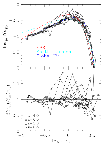
Figure 2: The scaled conditional mass functions. The two panels each show the twelve conditional mass functions of Fig. 1 expressed in terms of the variable $\nu_{12}=(\delta_{1}-\delta_{2})/(\sigma_{1}^{2}-\sigma_{2}^{2})^{1/2}$. The linked triangles, squares, pentagons and hexagons are the data from redshifts $z_{1}=0.5$, $1$, $2$ and $4$ respectively. In the top panel these scaled conditional mass functions are plotted logarithmically and compared to analytic functions. The solid curve is the EPS prediction, the dashed curve is the Sheth-Tormen mass function and the dotted curve is the Global Fit, $f_{\rm GF}(\nu_{12})$ (equation 7). The lower panel shows the ratio of each of the N-body estimates to the global fit, $f_{\rm GF}(\nu_{12})$, on a linear scale

Fig. 2 shows all the conditional mass functions of Fig. 1 as a function of the variable $\nu_{12}=(\delta_{1}-\delta_{2})/(\sigma_{1}^{2}-\sigma_{2}^{2})^{1/2}$. For each curve, the two lowest mass bins of Fig. 1, which are effected by the mass resolution of the simulation, are not plotted. Also, any occupied bins where $M_{1}/M_{2}>1$ are ignored as $\nu_{12}\rightarrow\infty$ as $M_{1}/M_{2}\rightarrow 1$. In the EPS formalism the conditional mass functions expressed in terms of this variable are universal. The EPS prediction is just $f_{\rm PS}(\nu_{12})$ and is shown by the solid curve. We see that the MS curves are not truly universal in that there is significant real scatter in this plot. However, the majority of the curves scatter around quite a tight locus which, however, is not well fit by the EPS curve.

The dashed curve in Fig. 2 shows the function

$$f_{\rm ST}(\nu)=A\sqrt{\frac{2a}{\pi}}\left[1+\left(\frac{1}{a\nu^{2}}\right)^{p}\right]\nu\exp(-a\nu^{2}/2),$$ (6)

with $A=0.322$, $a=0.707$ and $p=0.3$. If this function is used instead of $f_{\rm PS}$ in equation (2), the result is the Sheth & Tormen (2002) mass function which provides an excellent match to the mass function found in a wide range of N-body simulations (Jenkins et al., 2001). $f_{\rm ST}(\nu_{12})$ is not intended to be used as a model for the conditional mass function because the elliptical collapse model which motivates its form breaks the symmetry which we have invoked in writing the conditional mass functions as a function of $\nu_{12}$ (see section 2.5 of Sheth & Tormen, 2002). Nevertheless, it is interesting to see whether, when abused in this way, it provides a good model. Examining Fig. 2, we see that it does better than EPS at fitting the peak of the scaled conditional mass function, but it is too high at low $\nu_{12}$.

The dotted curve in Fig 2, labelled ‘Global Fit’, shows the fitting function,

$$f_{\rm GF}(\nu_{12})=0.4\ \nu_{12}^{3/4}\,\exp(-\nu_{12}^{3}/10).$$ (7)

While the factor $\nu_{12}^{3}$ in the exponential does not seem natural for Gaussian initial conditions, this was the simplest functional form we tried that sucessfully reproduces the low-$\nu_{12}$ power-law slope found in the MS and the position and sharpness of the high-$\nu_{12}$ peak and cutoff. The results of using this function instead of $f_{\rm PS}(\nu_{12})$ in equation (5) are shown by the dotted curves in Fig. 1. We see that over the mass and redshift range probed, this function provides quite a good fit to all the conditional mass functions in the MS and is a very significant improvement over the predictions of EPS formalism. The $f_{\rm PS}(\nu)$ and $f_{\rm ST}(\nu)$ functions both satisfy the normalization property,

$$\int_{0}^{\infty}f(\nu)\,\frac{d\nu}{\nu}=1,$$ (8)

but, for this fitting formula,

$$\int_{0}^{\infty}f_{\rm GF}(\nu)\,\frac{d\nu}{\nu}=\left(\frac{0.4}{3}\right)\ 10^{1/4}\ \Gamma(1/4)=0.8596.$$ (9)

This means that $14$% of the mass is not accounted for by this model of the progenitor mass function. Since $f_{\rm GF}(\nu)$ is just a fit over the range $0.15\mathrel{\hbox{\hbox to0.0pt{\hbox{\lower 4.0pt\hbox{$\sim$}}\hss}\hbox{$<$}}}\nu\mathrel{\hbox{\hbox to0.0pt{\hbox{\lower 4.0pt\hbox{$\sim$}}\hss}\hbox{$<$}}}3$ this could mean that the true function becomes shallower for $\nu\mathrel{\hbox{\hbox to0.0pt{\hbox{\lower 4.0pt\hbox{$\sim$}}\hss}\hbox{$<$}}}0.15$ or that some fraction of the mass is accreted as a truly smooth component. For many applications this distinction is of little importance.

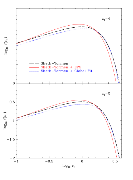
Figure 3: The Sheth-Tormen scaled mass function, $f_{\rm ST}(\nu_{1})$, at redshifts $z_{1}=2$ and $4$, compared with the scaled mass functions computed by combining two models of the conditional mass function in equation (10) with the Sheth-Tormen mass function at redshift $z_{2}=0$. In each panel, the dashed curve is the Sheth-Tormen mass function. The solid curve is the result of using the EPS conditional mass function and the dotted curve the result of using our fit, $f_{\rm GF}(\nu_{12})$. The upper panel shows redshift $z_{1}=4$ and the lower panel $z_{1}=2$.

In a self-consistent model, the overall mass function $f(M)$ and the conditional mass function $f(M_{1}|M_{2})$ must satisfy the constraint equation

$$f(M_{1})=\int_{M_{2}}f(M_{1}|M_{2})\ f(M_{2})\ d\ln M_{2}.$$ (10)

In other words, the total fraction of mass at the earlier epoch, $z_{1}$, in halos of mass $M_{1}$ must equal the fraction of mass of progenitors of mass $M_{1}$ coming from all the halos of mass $M_{2}$ at the later epoch, $z_{2}$. For the EPS formalism, equations (2) and (4), this is exactly true. If one considers scale-free models, i.e. a flat $\Omega_{\rm m}=1$ model with power-law initial conditions, $\sigma(M)\propto M^{-\alpha}$, then self-similarity (e.g. see Efstathiou et al., 1988) requires that this constraint equation can be written in the form

$$f(\nu_{1})=\int_{\nu_{2}=0}^{\infty}f(\nu_{1}|\,\nu_{2},\delta_{1}/\delta_{2})\ f(\nu_{2})\ d\ln\nu_{2},$$ (11)

where $\nu_{1}$ and $\nu_{2}$ are as defined earlier. In general, the form of the function $f(\nu_{1}|\,\nu_{2},\delta_{1}/\delta_{2})$ could depend on the slope of the power spectrum, and hence on $\alpha$, but one might hope this dependence is very weak in just the same way that the overall mass function, $f(M)$, is, to a very good approximation, universal when expressed as $f(\nu)$ (Sheth & Tormen, 1999; Jenkins et al., 2001). In seeking a universal conditional mass function in terms of the variable $\nu_{12}$, we are making the additional assumption that $f(\nu_{1}|\nu_{2},\delta_{1}/\delta_{2})$ can be replaced using the following substitution:

$$f(\nu_{1}|\nu_{2},\delta_{1}/\delta_{2})\rightarrow\left(\frac{\nu_{12}}{\nu_{1}}\right)^{2}\left(\frac{\delta_{1}/\delta_{2}}{\delta_{1}/\delta_{2}-1}\right)^{2}f(\nu_{12}),$$ (12)

where $\nu_{12}$ can be expressed as $\nu_{12}=(\delta_{1}-\delta_{2})/((\delta_{1}/\nu_{1})^{2}-(\delta_{2}/\nu_{2})^{2})^{1/2}$. This assumption, motivated by the extended Press-Schechter case, is not guaranteed to be true even in the self-similar case. Nevertheless, it is interesting to see how close our fitted universal conditional mass function, equation (7), comes to satisfying the constraint, when combined with the accurate Sheth-Tormen formula, equation (6), for both $f(\nu_{1})$ and $f(\nu_{2})$.

Note that in this case the constraint can be written as

$$\nu_{1}^{2}f(\nu_{1})=\left(\frac{\delta_{1}}{(\delta_{1}-\delta_{2})}\right)^{2}\int_{\nu_{2}=0}^{\infty}\nu_{12}^{2}\,f(\nu_{12})\ f(\nu_{2})\ d\ln\nu_{2},$$ (13)

which has no dependence on the form of $\sigma(M)$ and hence no dependence on the power spectrum. Thus, if one were to find a function, $f(\nu_{12})$, that satisfied this equation, it would produce a self-consistent conditional mass function for all power spectra and redshifts. Here, we merely examine the result of adopting the $f_{\rm GF}(\nu_{12})$ that we have found empirically by fitting to the MS data. The fact that $f_{\rm GF}(\nu_{12})$ does not satisfy the normalization constraint of equation (8) implies that it cannot satisfy equations (10) or (13) for all $\nu$. However, this does not necessarily prevent it from being accurate and self-consistent for the more massive progenitors, which are inherently the most interesting.

In Fig. 3 we perform this comparison. The mass functions at the epochs $z_{1}=2$ and $4$ are plotted in terms of the scaled variable $\nu_{1}$. In this variable, the Sheth-Tormen mass function is the same at all redshifts and for all power spectra. These mass functions are compared with the result of computing $f(\nu_{1})$ from equation (13) using both the EPS conditional mass function and our Global Fit. We see that neither is fully consistent, but that our fit does a better job of matching the Sheth-Tormen curve than using the EPS formula and is particularly good for the highest masses (high $\nu_{1}$). Experimentation showed that it is possible to find a modified $f(\nu_{12})$ that leads to results more consistent with the Sheth-Tormen mass function, but in that case $f(\nu_{12})$ produces noticeably poorer matches to the MS conditional mass functions plotted in Fig. 1. We take this as an indication that in reality the conditional mass function is not strictly universal and that the ansatz (12) is an imperfect approximation. However, it remains true that our fitting function, equation (7), is a good approximation to the MS results over the mass and redshift range probed in Fig. 1 and that, when applied to all masses, it continues to produce results that are more self-consistent than using the equivalent EPS formula, as indicated in Fig. 3. We would expect this improvement over the EPS formula to continue to hold for all variants of the $\Lambda$CDM model and even for hierarchical models with very different power spectra.

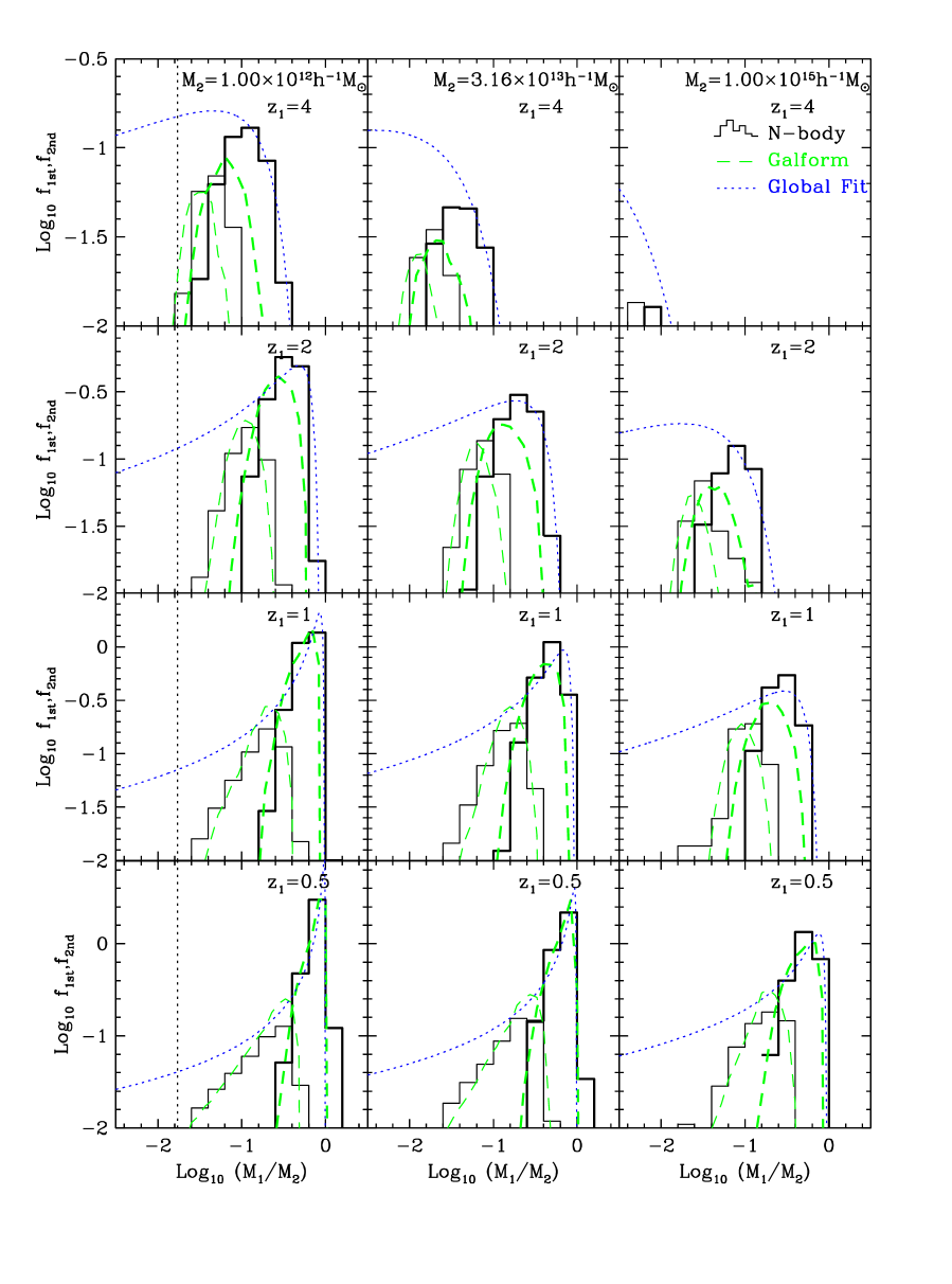
Figure 4: The mass distributions of the first and second most massive progenitors. The plotted quantities $f_{\rm 1st}$ and $f_{\rm 2nd}$ are the contributions to the overall conditional mass functions plotted in Fig. 1 provided by the 1st and 2nd most massive progenitors respectively. The panels correspond directly to those of Fig. 1 and are labelled by the final halo mass $M_{2}$ and redshift $z_{1}$ of the progenitors. The histograms show the results from the Millennium Simulation with the distribution $f_{\rm 1st}$ plotted with heavy lines and $f_{\rm 2nd}$ with light lines. The corresponding predictions of the GALFORM Monte-Carlo algorithm are shown by the heavy and light dashed curves. The dotted curves are the same Global Fit to the conditional mass function that were plotted in Fig. 1, but note that the scales on both the $x$ and $y$ axes are different. They are plotted here as reference lines. The $20$ particle mass resolution of the Millennium Simulation is shown by the vertical dotted line, but only plays a role for the $z=4$ progenitors of the lowest mass, $M_{2}=10^{12}$ M_⊙, halos.

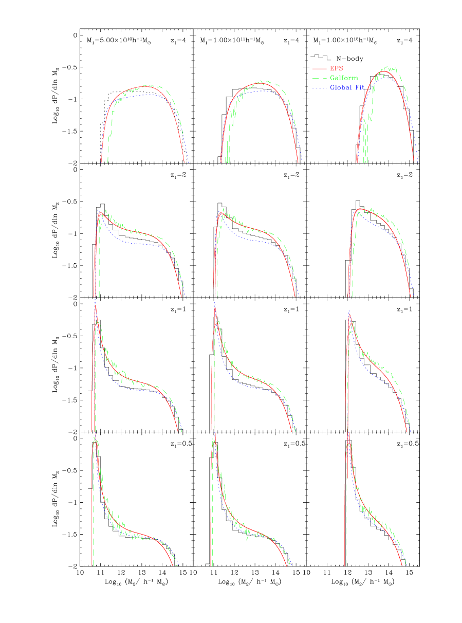
Figure 5: The distribution of final halo masses, $M_{2}$, in which halos of mass $M_{1}$ that exist at redshift $z_{1}$ find themselves at redshift $z_{2}=0$. As labelled on the panels, each column is for a different progenitor mass, $M_{1}$, and each row for a different progenitor redshift, $z_{1}$. The histograms show the result for the MS, the solid curves the prediction of EPS formalism, the dashed lines the result of the GALFORM Monte-Carlo algorithm, and the dotted line the prediction of the “Global Fit” model of equation (7), combined with the Sheth-Tormen mass function as described in the text.

4.2 Main Progenitor Mass Functions

Although the conditional mass functions discussed above are interesting functions which can be modelled analytically, often of more importance in galaxy formation models are the properties of the most massive progenitors of a given halo. Fig 4 shows the mass distribution of the first and second most massive progenitors for the same final halo masses and redshifts as in Fig. 1. These mass functions are subsets of the overall conditional mass function in the sense that $f_{\rm cmf}=f_{\rm 1st}+f_{\rm 2nd}+f_{\rm 3rd}...$ . The functions $f_{\rm 1st}$ and $f_{\rm 2nd}$ can easily be related to the probability distributions for the masses of the first and second ranked progenitors. For instance, for a halo of mass $M_{2}$ at redshift $z_{2}=0$, the probability that its most massive progenitor at redshift $z_{1}$ has mass $M_{1}$ in the interval $d\log M_{1}$ is proportional to $(M_{2}/M_{1})f_{\rm 1st}\,d\log M_{1}$.

In the MS we see normal hierarchical behaviour with the typical mass of both the first and second most massive progenitors decreasing with redshift. This rate of decrease is greatest for the halos with the largest present day mass, i.e. for high $M/M_{*}$ halos (where as usual the characteristic mass, $M_{*}$, is defined by $\sigma(M_{*})=\delta$). It is striking that the mass distribution of the 1st ranked progenitors becomes very narrow at high redshift for high mass descendants. However, this is to be expected when the most massive progenitor is much less massive than the final object – one has many progenitors to choose from and the most massive one will always be close to the upper mass exponential cut off of the distribution. By comparing to the dotted curves, which show the “Global Fit” to the total mass functions of Fig. 1, we can see the mass ranges over which the first and second most massive progenitor make the dominate contribution to the overall conditional mass functions.

The dashed curves show the corresponding results for the GALFORM Monte-Carlo merger trees. These agree very well with the MS at low redshift. The typical widths of the distributions of both the first and second ranked progenitors and the relative masses of their peaks all exhibit similar mass and redshift dependence to the simulation. However, as was the case for the overall conditional mass function, the evolution of the typical mass with redshift is too rapid. At redshift $z_{1}=4$ the typical mass of both the first and second ranked progenitor is about a factor two less than the corresponding mass found in the MS.

4.3 Final Mass Distributions

In relating observations of the high redshift Universe to the present day one would often like to know where, for a given class of observed high redshift object, will their descendant reside today. One step towards answering this question is to quantify the fate of high redshift halos in terms of the halos into which they become incorporated by the present day. Thus, we have selected halos of mass $M_{1}$ at redshift $z_{1}$ and followed their merger histories until the present, $z_{2}=0$, and for each one recorded the final halo mass $M_{2}$. Fig 5 shows the probability distribution, $dP/d\ln M_{2}$, that this final mass is in a given range of $\ln M_{2}$ and is plotted for initial redshifts $z_{1}=0.5,1,2$ and $4$ and initial masses $M_{1}=5\times 10^{10}$, $10^{11}$ and $10^{12}$ M_⊙. For low redshifts $z_{1}$, the distributions have the form of a peak around the original halo mass plus a shoulder extending up to the mass of the highest mass halos present at $z=0$. As the redshift increases the low mass peak declines and the shoulder grows until it dominates the distribution. These general features are reproduced well by both the EPS formalism and the GALFORM Monte-Carlo algorithm whose distributions are shown, respectively, by the solid and dashed curves on Fig 5, but both have shoulders that slope somewhat more steeply than those of the MS distributions. Consistent with the mismatch that was noted between the GALFORM and EPS distributions in Fig 1, we see that the GALFORM distributions are shifted slightly to higher masses than the corresponding EPS distribution.

This EPS prediction for the probability $dP/d\ln M_{2}$ is simply proportional to the fraction of mass that is in halos of mass $M_{1}$ at $z_{1}$ that ends up in halos of $M_{2}$ at $z_{2}$ and can be computed using the probability product rule

$$f(M_{2}|M_{1})\,d\ln M_{2}=\frac{f(M_{1}|M_{2})\,d\ln M_{1}\ f(M_{2})\,d\ln M_{2}}{f(M_{1})\,d\ln M_{1}}$$ (14)

(Lacey & Cole, 1993). Using the notation defined above this can be written as

$$f(M_{2}|M_{1})\,d\ln M_{2}=$$ (15)

$$\frac{f_{\rm PS}(\nu_{12})\left|\frac{d\ln\nu_{12}}{d\ln M_{1}}\right|\,f_{\rm PS}(\nu_{2})\left|\frac{d\ln\nu_{2}}{d\ln M_{2}}\right|d\ln M_{2}}{f_{\rm PS}(\nu_{1})\left|\frac{d\ln\nu_{1}}{d\ln M_{1}}\right|}.$$

It is interesting to see the effect of replacing $f_{\rm PS}(\nu_{12})$ with the fitting function that we obtained for the conditional mass function (equation 7) and the other two occurrences of $f_{\rm PS}(\nu)$ with Sheth & Tormen’s fit to the mass function. The resulting distribution

$$f(M_{2}|M_{1})\,d\ln M_{2}\rightarrow$$ (16)

$$\frac{f_{\rm GF}(\nu_{12})\left|\frac{d\ln\nu_{12}}{d\ln M_{1}}\right|\,f_{\rm ST}(\nu_{2})\left|\frac{d\ln\nu_{2}}{d\ln M_{2}}\right|d\ln M_{2}}{f_{\rm ST}(\nu_{1})\left|\frac{d\ln\nu_{1}}{d\ln M_{1}}\right|}.$$

is shown by dotted curves shown in Fig. 5. While not perfect, this function is in distinctly better agreement with the MS results than the EPS formalism and should serve as a useful analytic description of the fate of high redshift dark matter halos in $\Lambda$CDM models.

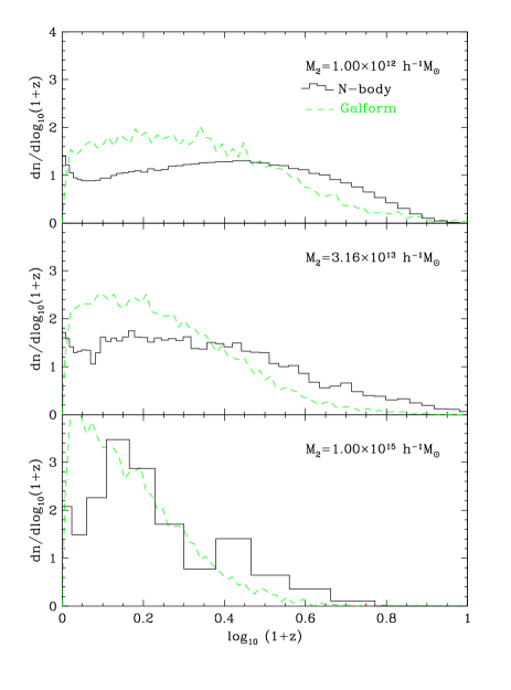
Figure 6: The redshift distribution of the most recent major merger of halos with different final masses $M_{2}$. The solid curves show the distributions for the MS halos and the dashed curves the corresponding distributions from the GALFORM Monte-Carlo algorithm.

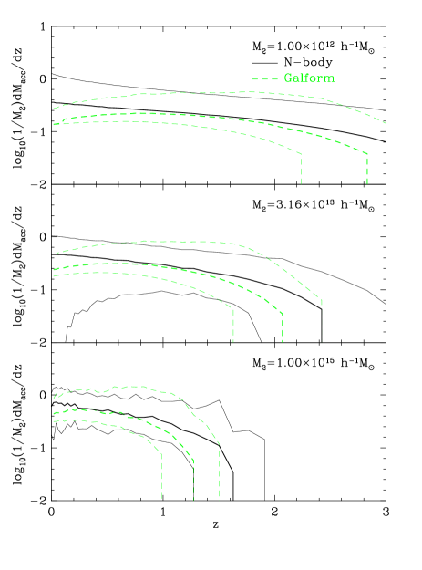
Figure 7: The normalized accretion rate $({1}/{M_{2}})({dM_{\rm acc}}/{dz})$ as a function of redshift for halos within a factor of two of the final masses $M_{2}=1.0\times 10^{12}$, $3.16\times 10^{13}$ and $1.0\times 10^{15}$ M_⊙. The heavy solid curve shows the median rates for $X=0.1$ and the outer lighter solid curves indicate the 20 and 80 percentiles of the distribution. The heavy and light dashed curves shows the corresponding results for the GALFORM Monte-Carlo method.

4.4 Major Mergers

Major mergers of comparable mass halos and comparable mass galaxies play an important role in many galaxy formation models. Such mergers are usually invoked to explain the formation of galactic bulges and elliptical galaxies. The frequency and redshift distribution of major mergers are of particular interest. Fig. 6 shows the distribution, for halos of final mass $M_{2}$, of the redshift at which their most massive progenitor most recently underwent a merger with another halo of mass greater than $f_{\rm major}=0.3$ times its own mass. The distribution is broadest for low mass halos, such that, for halos of mass $M_{2}=10^{12}$M_⊙, 10% have a major merger at $z<0.1$ while another 10% have not had one since $z>3.7$. As the mass of the final halo increases, the most recent major merger tends to occur more and more recently although even for halos of mass $M_{2}=3.16\times 10^{13}h^{-1}$ M_⊙the redshift distribution is still quite extended.

The dashed lines in Fig 6 show the corresponding predictions of the GALFORM Monte-Carlo algorithm. While the mass dependence of the widths of the distributions is reproduced, the predictions differ significantly from the MS results. The Monte-Carlo algorithm significantly overestimates the number of recent major mergers. This is in the same sense as the overly rapid evolution of the conditional mass functions seen in Fig. 1, but is more pronounced.

4.5 Accretion Rates

Although in the $\Lambda$CDM cosmology halos buildup via mergers, the mass distribution of the merging fragments is very broad and even at redshift $z=0$ a significant fraction of a halo’s mass is accreted as small objects. The statistics on which we have focused above stress the role of the more massive progenitors in a halo merger tree, but sometimes the lower mass progenitors can bring in significant amounts of mass and play an important role. For instance, accretion rates derived from the EPS formalism were computed by Miller et al. (2006) and compared to high redshift N-body simulations by Cohn & White (2007) with the aim of obtaining accretion rates onto supermassive black holes and studying reionization. Also, if photoionization prevents cooling and consequently star formation in halos below a certain mass (e.g. Gnedin, 2000; Benson et al., 2002), then the accretion of such low mass halos can be an important source of primordial unenriched material. In Fig. 7 we plot a normalized accretion rate as a function of redshift for halos of various final masses. We have set a mass threshold of $X=0.1$ times $M_{2}$ and consider the accretion of mass in all halos below this threshold onto halos with masses greater than this threshold.

In Fig. 7, we see some significant differences between the results for the GALFORM Monte-Carlo algorithm and the MS merger trees. Both sets of trees show the same trend for the accretion to be more concentrated at low redshifts for the highest mass halos. The median accretion rates of the two sets of trees are in good a agreement at intermediate redshifts, but the MC algorithm underpredicts the accretion at both high and low redshift. However, we note that estimating this statistic from the MS is problematic. As noted earlier, for our simple FOF merger trees, there are occasions when halo growth is not hierarchical and halo masses can go down as well as up. For instance, this can happen when halos are temporarily linked by the FOF algorithm before splitting apart and then perhaps merging again later on. Since we are plotting a differential statistic this “noise” does not average out over time. As noted in the discussion of Fig. 1, the problem is largely confined to low mass halos, but since we are focusing here on the lowest mass halos it can have a significant effect. In fact, the reason that no 20 percentile line is visible in the upper panel of Fig. 7 is that for these low mass merger trees 20 per cent loose mass in a given time step.

5 Conclusions

The Millennium Simulation (MS, Springel et al., 2005a) is a powerful resource for the statistical study of the hierarchical growth of structure. For ease of reproduction and clarity of definition, we have studied halos defined by the friends-of-friends group finding algorithm (Davis et al., 1985) with a linking length parameter $b=0.2$ . For these halos the statistics we have presented represent a comprehensive summary of their formation histories and are all available in electronic form at http://star-www.dur.ac.uk/$\tilde{\hphantom{n}}$cole/merger_trees . Their comparison with the predictions of Extended Press-Schechter (EPS) formalism and the GALFORM Monte-Carlo extension are illuminating.

All the models to which we compare the simulation data make the assumption that halo merger histories depend solely on the final halo mass and not on any additional property such as its environment. However, previous studies of the MS (Gao et al., 2005; Harker et al., 2006; Gao & White, 2007) have shown that this is not the case. Gao et al. (2005) found that the two-point correlation function of halos of a given mass depends on halo formation time, while Harker et al. (2006) reached a similar conclusion using a marked correlation function analysis to probe the environmental dependence of halo formation time (see also Sheth & Tormen, 2004). Nevertheless, for many applications it is adequate to ignore such dependencies and merely have a model that fits the mean statistics averaged over all environments. For instance, the prediction of galaxy luminosity functions and how they evolve with redshift does not require modelling the environmental dependence. On the other hand, the environmental dependence of halo merger trees is important when making predictions of halo or galaxy clustering (Croton et al., 2007), although the effects are weak for all but special subsets of galaxies. Even in these cases, there are techniques that allow one to make use of the average merger trees studied here (e.g. by using an effective mass that is modulated by environment Harker et al., 2007).

The EPS theory represents the only fully analytic model of the hierarchical growth of structure. While its derivation requires making several gross approximations and assumptions (Bond et al., 1991; Lacey & Cole, 1993), it is remarkable that it captures well the qualitative dependences of progenitor mass distributions on redshift and final halo mass and of final halo mass distributions on initial progenitor mass and redshift. However, its accuracy is not sufficient for the present era of precision cosmology. For example, at high redshift, $z=4$, it can underestimate the typical progenitor mass by factors of $3$ or $4$, or equivalently the abundance of the most massive progenitors by factors of a few (see Fig. 1). Hence, just as the fits of Jenkins et al. (2001) and Sheth et al. (2001) have become the descriptions of choice for the halo mass function, there is now a need for a more accurate description of these conditional mass functions. The analytic fitting function we have presented here largely achieves this. While the conditional mass functions when expressed in the scaling parameter, $\nu_{12}=(\delta_{1}-\delta_{2})/((\sigma_{1}^{2}-\sigma_{2}^{2})^{1/2}$, do exhibit systematic deviations from a universal form, the deviations are relatively small. In particular, their scatter is smaller than the systematic offset between them and the EPS prediction. Hence, adopting our fit and using it as a universal conditional mass function results in quite accurate reproductions of all the halo conditional progenitor and descendant mass distributions. Although this fit was made using just one $\Lambda$CDM simulation and so is probably not optimal for models with significantly different power spectra, we would still, even in these cases, expect it to be a significant improvement over the EPS theory.

Realizations of individual halo merger trees or predictions of more complex statistical properties of halo merger trees cannot be made using EPS theory (or our fitted universal conditional mass function) without making additional assumptions and approximations. In the case of the GALFORM Monte-Carlo algorithm, whose trees we have compared with those of the MS, these additional assumptions prevent it from being fully self-consistent with the EPS theory. The root of this inconsistency is the asymmetry in the predicted merger rate of halos of mass $M$ and $M_{2}-M$ when forming a halo of mass $M_{2}$ (Lacey & Cole, 1993; Sheth & Pitman, 1997; Cole et al., 2000; Benson et al., 2005) that is implicit in the EPS formalism. The practical consequence of this is that the typical halo mass in the Monte-Carlo trees evolves more rapidly with redshift than the corresponding EPS prediction. This increases the discrepancy between the conditional mass functions of the model and those of the MS. This is the main shortcoming of the GALFORM Monte-Carlo algorithm, as in other statistical properties that cannot be predicted by the pure EPS theory, it continues to provide a good qualitative description of the MS halo statistics. For instance, the distributions of the first and second most massive progenitors have shapes, widths and relative positions that mirror well those of the MS, but are systematically displaced to lower masses at high redshift. Overcoming this one shortcoming of the algorithm would produce much better agreement with the simulation results. However, the task of defining a fully self-consistent algorithm is extremely challenging (Benson et al., 2005). Instead, in Parkinson, Cole & Helly (2007), we will take a more pragmatic approach and explore whether minor modifications to the GALFORM Monte-Carlo algorithm can produce a better match to the MS data.

References

- Baugh et al. (2005) Baugh, C. M., Lacey, C. G., Frenk, C. S., Granato, G. L., Silva, L., Bressan, A., Benson, A. J., Cole, S. 2005, MNRAS, 356, 1191
- Benson et al. (2001) Benson, A. J., Pearce, F. R., Frenk, C. S., Baugh, C. M., Jenkins, A. 2001, MNRAS, 320, 261
- Benson et al. (2002) Benson, A. J., Lacey, C. G., Baugh, C. M., Cole, S., & Frenk, C. S. 2002, MNRAS, 333, 156
- Benson et al. (2003) Benson, A. J., Bower, R. G., Frenk, C. S., Lacey, C. G., Baugh, C. M., Cole, S. 2003, ApJ, 599, 38
- Benson et al. (2005) Benson, A. J., Kamionkowski, M., Hassani, S. H. 2005, MNRAS, 357, 847
- Bond et al. (1991) Bond, J. R., Cole, S., Efstathiou, G., Kaiser, N. 1991, ApJ, 379, 440
- Bower (1991) Bower, R. G. 1991, MNRAS, 248, 332
- Bower et al. (2006) Bower, R. G., Benson, A. J., Malbon, R., Helly, J. C., Frenk, C. S., Baugh, C. M., Cole, S., Lacey, C. G. 2006, MNRAS, 370, 645
- Cohn & White (2007) Cohn, J. D., & White, M. 2007, astro-ph/07060208
- Cole (1991) Cole, S. 1991, ApJ, 367, 45
- Cole et al. (2000) Cole, S., Lacey, C. G., Baugh, C. M., Frenk, C. S. 2000, MNRAS, 319, 168
- Croton et al. (2006) Croton, D. J., et al. 2006, MNRAS, 365, 11
- Croton et al. (2007) Croton, D. J., Gao, L., White, S. D. M. 2007, MNRAS, 374, 1303
- Davis et al. (1985) Davis, M., Efstathiou, G., Frenk, C. S., White, S. D. M. 1985, ApJ, 292, 371
- De Lucia et al. (2006) De Lucia, G., Springel, V., White, S. D. M., Croton, D., Kauffmann, G. 2006, MNRAS, 366, 499
- Efstathiou et al. (1988) Efstathiou, G., Frenk, C. S., White, S. D. M., Davis, M. 1988, MNRAS, 235, 715
- Eke et al. (1996) Eke, V. R., Cole, S., Frenk, C. S. 1996, MNRAS, 282, 263
- Epstein (1983) Epstein, R. I. 1983, MNRAS, 205, 207
- Gao et al. (2004) Gao, L., White, S. D. M., Jenkins, A., Stoehr, F., & Springel, V. 2004, MNRAS, 355, 819
- Gao et al. (2005) Gao, L., Springel, V., & White, S. D. M. 2005, MNRAS, 363, L66
- Gao & White (2007) Gao, L., White, S. D. M. 2007, MNRAS, 377, L5
- Giocoli et al. (2007) Giocoli, C., Moreno, J., Sheth, R. K., & Tormen, G. 2007, MNRAS, 376, 977
- Gnedin (2000) Gnedin, N. Y. 2000, ApJ, 542, 535
- Harker et al. (2006) Harker, G., Cole, S., Helly, J. C., Frenk, C., Jenkins, A. 2006, MNRAS, 367, 1039
- Harker et al. (2007) Harker, G., 2007, University of Durham thesis.
- Helly et al. (2003) Helly, J. C., Cole, S., Frenk, C. S., Baugh, C. M., Benson, A., Lacey, C. 2003, MNRAS, 338, 903
- Kauffmann & White (1993) Kauffmann, G., White, S. D. M. 1993, MNRAS, 261, 921
- Jenkins et al. (2001) Jenkins, A., Frenk, C. S., White, S. D. M., Colberg, J. M., Cole, S., Evrard, A. E., Couchman, H. M. P., Yoshida, N. 2001, MNRAS, 321, 372
- Lacey & Cole (1993) Lacey, C., Cole, S. 1993, MNRAS, 262, 627
- Lacey & Cole (1994) Lacey, C., Cole, S. 1994, MNRAS, 271, 676
- Li et al. (2007) Li, Y., Mo, H. J., van den Bosch, F. C., & Lin, W. P. 2007, MNRAS, 379, 689
- Lin et al. (2003) Lin, W. P., Jing, Y. P., & Lin, L. 2003, MNRAS, 344, 1327
- Miller et al. (2006) Miller, L., Percival, W. J., Croom, S. M., & Babić, A. 2006, A&A, 459, 43
- Parkinson, Cole & Helly (2007) Parkinson, H., Cole, S., Helly, J. C. 2007, MNRAS, submitted.
- Percival et al. (2001) Percival, W. J., et al. 2001, MNRAS, 327, 1297
- Press & Schechter (1974) Press, W. H., Schechter, P. 1974, ApJ, 187, 425
- Sánchez et al. (2006) Sánchez, A. G., Baugh, C. M., Percival, W. J., Peacock, J. A., Padilla, N. D., Cole, S., Frenk, C. S., & Norberg, P. 2006, MNRAS, 366, 189
- Sheth (1996) Sheth, R. K. 1996, MNRAS, 281, 1277
- Sheth & Pitman (1997) Sheth, R. K., & Pitman, J. 1997, MNRAS, 289, 66
- Sheth & Lemson (1999) Sheth, R. K., & Lemson, G. 1999, MNRAS, 305, 946
- Sheth & Tormen (1999) Sheth, R. K., & Tormen, G. 1999, MNRAS, 308, 119
- Sheth et al. (2001) Sheth, R. K., Mo, H. J., Tormen, G. 2001, MNRAS, 323, 1
- Sheth & Tormen (2002) Sheth, R. K., Tormen, G. 2002, MNRAS, 329, 61
- Sheth & Tormen (2004) Sheth, R. K., & Tormen, G. 2004, MNRAS, 350, 1385
- Somerville & Kolatt (1999) Somerville, R. S., & Kolatt, T. S. 1999, MNRAS, 305, 1
- Spergel et al. (2003) Spergel, D. N., et al. 2003, ApJS, 148, 175
- Spergel et al. (2007) Spergel, D. N., et al. 2007, ApJS, 170, 377
- Springel et al. (2001) Springel, V., White, S. D. M., Tormen, G., Kauffmann, G. 2001, MNRAS, 328, 726
- Springel et al. (2005a) Springel, V., et al. 2005a, Nature, 435, 629
- Springel (2005b) Springel, V. 2005b, MNRAS, 364, 1105
- van den Bosch (2002) van den Bosch, F. C. 2002, MNRAS, 331, 98
- Wechsler et al. (2002) Wechsler, R. H., Bullock, J. S., Primack, J. R., Kravtsov, A. V., & Dekel, A. 2002, ApJ, 568, 52