A Closure Theory for Non-linear Evolution of Cosmological Power Spectra

Atsushi Taruya, Takashi Hiramatsu Research Center for the Early Universe (RESCEU), School of Science, The University of Tokyo, Tokyo 113-0033, Japan.
Abstract

We apply a non-linear statistical method in turbulence to the cosmological perturbation theory and derive a closed set of evolution equations for matter power spectra. The resultant closure equations consistently recover the one-loop results of standard perturbation theory and beyond that, it is still capable of treating the non-linear evolution of matter power spectra. We find the exact integral expressions for the solutions of closure equations. These analytic expressions coincide with the renormalized one-loop results presented by Crocce & Scoccimarro (2006a, 2007), apart from the vertex renormalization. By constructing the non-linear propagator, we analytically evaluate the non-linear matter power spectra based on the first-order Born approximation of the integral expressions and compare it with those of the renormalized perturbation theory.

Subject headings:
cosmology:theory–dark matter–large-scale structure of universe

1. Introduction

Cosmology now enters the era of precision cosmology. With large data set from the precision measurements of the cosmic microwave background anisotropies as well as the matter density fluctuations in the large-scale structure, the standard cosmological model has been fully established (e.g., Spergel et al., 2006; Tegmark et al., 2006). The associated cosmological parameters are well-determined with an accuracy of less than 10%percent1010\% level. With improved sensitivity and higher precision of future observations, the modern picture of the universe will be further reinforced and one can even explore a tiny signature of new physics beyond the standard cosmological model.

In fact, several ambitious missions for galaxy redshift survey are planed in order to reveal the nature of dark energy (e.g., Albrecht et al., 2006; Peacock et al., 2006, and references therein). Among these, Wide-field Fiber-fed Multi-Object Spectrograph (WFMOS) may be one of the best facility capable of achieving the percent-level measurement of baryon acoustic oscillations (BAOs) imprinted in the matter power spectrum (Meiksin, White & Peacock, 1999). The recent observations from Sloan Digital Sky Survey (SDSS) and Two-degree-Field Galaxy Redshift Survey (2dF GRS) showed that the characteristic scale of BAOs can be used as the cosmic standard ruler to determine the distance-redshift relation of high-redshift galaxies (Cole et al., 2005; Eisenstein et al., 2005; Hütsi, 2006; Percival et al., 2007). Since the distance-redshift relation is sensitive to the cosmic expansion history, details of the accelerated expansion can be clarified from the accurate measurement of BAOs (Seo & Eisenstein, 2003). With percent-level measurement of characteristic scale of BAOs, the determination of dark energy equation-of-state, parametrized by wPde/ρde𝑤subscript𝑃desubscript𝜌dew\equiv P_{\rm de}/\rho_{\rm de}, will achieve a few percent accuracy, where Pdesubscript𝑃deP_{\rm de} and ρdesubscript𝜌de\rho_{\rm de} are the pressure and the energy density of dark energy, respectively.

On the other hand, pursuit of the nature of dark energy highlights various fundamental problems which are potentially crucial for the accurate determination of dark energy equation-of-state. For example, the observation of BAOs requires high-precision theoretical template for the matter power spectrum in the relevant wavenumber, k0.10.3hsimilar-to𝑘0.10.3k\sim 0.1-0.3hMpc-1. To achieve the required accuracy in the determination of w𝑤w, several systematic effects must be incorporated into the theoretical predictions. Among known systematic effects, the non-linear gravitational clustering is one of the most fundamental building block in the theory of structure formation. The recent N𝑁N-body simulations showed that the non-linear growth of matter distribution significantly alters the shape of the power spectrum and the acoustic signature of BAOs tends to be erased, where linear theory prediction of matter power spectrum is no longer valid (e.g., Meiksin, White & Peacock, 1999; Seo & Eisenstein, 2005). To tackle the issue, the perturbation theory for gravitational clustering has been revived and has been applied to the study of BAOs (e.g., Suto & Sasaki, 1991; Makino, Sasaki & Suto, 1992; Jain & Bertschinger, 1994; Scoccimarro & Frieman, 1996; Jeong & Komatsu, 2006; Nishimichi et al., 2007). The inclusion of leading-order correction to the non-linear clustering effect somehow improves a performance and reproduces the N𝑁N-body results very well (Jeong & Komatsu, 2006). At lower redshifts z<2𝑧2z<2, however, next-to-leading order effect becomes important and the theoretical prediction with leading-order correction is insufficient to reproduce the N𝑁N-body simulations.

Going beyond the perturbation theory, existing theoretical tools dealing with the non-linear gravitational clustering are the N𝑁N-body simulation and the fitting formula for matter power spectrum (e.g., Peacock & Dodds, 1996; Smith et al., 2003), as well as the phenomenological approach based on the halo model (Cooray & Sheth, 2002, for a review). Currently, however, none of the reliable methods to ensure the percent-level precision exist. While the N𝑁N-body simulation has a potential to provide a high-precision prediction, at present, one cannot blindly trust the N𝑁N-body results unless reliable and comparable counterpart is established and is fully reconciled with N𝑁N-body results. In this respect, development of new analytical method beyond the perturbation theory is necessary and essential for the progress on precision cosmology.

In this paper, we present a non-linear statistical method to predict the time evolution of matter power spectrum. Very recently, there appear several works on the statistical treatment going beyond the perturbation theory (Valageas, 2004; Crocce & Scoccimarro, 2006a, b; McDonald, 2007; Valageas, 2007a; Matarrese & Pietroni, 2007; Izumi & Soda, 2007). Based on the field-theoretical approach, the perturbation theory has been reformulated by improving the summation of the naive perturbative expansion. The so-called renormalized perturbation theory (RPT) developed by Crocce & Scoccimarro (2006a) seems viable theoretical tool alternative to the N𝑁N-body simulation, suited to a high-precision prediction. Using RPT, some attempts to predict the non-linear evolution of BAOs has been reported (Crocce & Scoccimarro, 2007). Here, we consider an alternative statistical method accepted widely in the subject of statistical theory of turbulence (e.g., Kraichnan, 1959; Leslie, 1973; Kaneda, 1981; Kida & Goto, 1997). In contrast to the sophisticated treatment based on the field-theoretical approach, our method is rather primitive in the sense that the effect of non-linearity of matter power spectrum is simply described by a systematic expansion and a truncation of the naive perturbation. After applying the so-called reversed expansion, the perturbative expansion is effectively re-organized and a class of higher-order corrections is systematically re-summed (Wyld, 1961). With this treatment, some non-perturbative effects are also incorporated. We derive a closed set of moment equations characterizing the non-linear evolution of power spectra. The resultant evolution equations consistently recover the leading-order results of standard perturbation theory (one-loop PT). The solutions for these closure equations have exact integral expressions, which coincides with the one-loop results of RPT. Constructing the non-linear propagator, we attempt to evaluate the non-linear matter power spectra analytically. Based on the first-order Born approximation of the exact integral expressions, we find that the power spectra from the closure theory reasonably agree with those from the RPT.

The outline of the paper is as follows. In Section 2, governing equations for the dynamics of cosmological gravitational clustering is presented on the basis of the fluid description of the Vlasov equation. The closure problem, i.e., theoretical issue on the self-consistent treatment of the hierarchy of moment equations, is briefly mentioned. In Section 3, non-linear statistical method in turbulence called direct interaction approximation is introduced and is applied to the present cosmological situation. Then, a closed set of evolution equations for matter power spectrum is obtained by the systematic perturbative expansion and the so-called reversion procedure. In Section 4, important properties of the resultant closure equations, i.e., recovery of standard PT and exact integral solutions, are discussed, based on detailed mathematical calculations presented in Appendices A and B. In Section 5, analytical treatment for our closure system is presented for illustrative purpose. Constructing approximate solutions for non-linear propagator, power spectrum of density fluctuations is calculated based on the Born approximation of the integral solutions. The results are compared with those obtained from RPT, particularly focusing on the non-linear evolution of BAOs. Finally, Section 6 is devoted to discussion and conclusions.

2. Preliminaries

2.1. Basic equations

Throughout the paper, we consider the evolution of mass distribution in the flat universe, neglecting the tiny contribution from the massive neutrinos. To evaluate the non-linear growth of the density perturbations, hydrodynamic description of mass distribution is useful. Strictly speaking, this treatment is not exact and is often called the single-stream approximation of the Vlasov equation. However, at least in a statistical sense, it would be the best approximation if the scale of our interest is sufficiently large so that one can safely ignore the effect of shell-crossing. Denoting the fluctuation of mass distribution consisting of the cold dark matter and the baryon fluid by δ𝛿\delta, we have

δt+1a{(1+δ)𝒗}=0,𝛿𝑡1𝑎1𝛿𝒗0\displaystyle\frac{\partial\delta}{\partial t}+\frac{1}{a}\,\nabla\{(1+\delta)\mbox{\boldmath$v$}\}=0, (1)
𝒗t+H𝒗+1a(𝒗)𝒗=1aϕ,𝒗𝑡𝐻𝒗1𝑎𝒗𝒗1𝑎italic-ϕ\displaystyle\frac{\partial\mbox{\boldmath$v$}}{\partial t}+H\mbox{\boldmath$v$}+\frac{1}{a}\,(\mbox{\boldmath$v$}\cdot\nabla)\mbox{\boldmath$v$}=-\frac{1}{a}\,\nabla\phi, (2)
1a22ϕ=4πGρmδ1superscript𝑎2superscript2italic-ϕ4𝜋𝐺subscript𝜌m𝛿\displaystyle\frac{1}{a^{2}}\,\nabla^{2}\phi=4\pi\,G\,\rho_{\rm m}\,\delta (3)

Here, a𝑎a is the scale factor of the universe, H𝐻H is the Hubble parameter and ρmsubscript𝜌m\rho_{\rm m} is the homogeneous mass density field. Assuming the irrotationality of the fluid flow, the above equations can be recast as (e.g., Taruya, 2000):

δt+Hθ+1a(δ𝒗)=0,𝛿𝑡𝐻𝜃1𝑎𝛿𝒗0\displaystyle\frac{\partial\delta}{\partial t}+H\,\theta+\frac{1}{a}\nabla(\delta\cdot\mbox{\boldmath$v$})=0, (4)
θt+12(13wΩw)Hθ+1a2H{(𝒗)𝒗}+32H(1Ωw)δ=0,𝜃𝑡1213𝑤subscriptΩ𝑤𝐻𝜃1superscript𝑎2𝐻𝒗𝒗32𝐻1subscriptΩ𝑤𝛿0\displaystyle\frac{\partial\theta}{\partial t}+\frac{1}{2}\left(1-3w\,\Omega_{w}\right)H\,\theta+\frac{1}{a^{2}H}\,\nabla\cdot\left\{(\mbox{\boldmath$v$}\cdot\nabla)\mbox{\boldmath$v$}\right\}+\frac{3}{2}H(1-\Omega_{w})\delta=0, (5)

where the quantity θ𝜃\theta is the velocity divergence defined by

θ=𝒗aH.𝜃𝒗𝑎𝐻\theta=\frac{\nabla\cdot\mbox{\boldmath$v$}}{aH}. (6)

The quantity ΩwsubscriptΩ𝑤\Omega_{w} is the density parameter of dark energy satisfying the equation of sate, Pde=wρdesubscript𝑃de𝑤subscript𝜌deP_{\rm de}=w\rho_{\rm de}, defined by Ωw=8πGρde/(3H2)subscriptΩ𝑤8𝜋𝐺subscript𝜌de3superscript𝐻2\Omega_{w}=8\pi\,G\,\rho_{\rm de}/(3H^{2}). Note that the relation Ωm+Ωw=1subscriptΩmsubscriptΩ𝑤1\Omega_{\rm m}+\Omega_{w}=1 holds in the flat cosmology.

To treat the non-linear evolution of the matter power spectrum, the Fourier representation of equations (4) and (5) is useful. To do this, we introduce the Fourier transform of the perturbed quantities:

δ(𝒙;t)=d3𝒌(2π)3ei𝒌𝒙δ(𝒌;t),θ(𝒙;t)=d3𝒌(2π)3ei𝒌𝒙θ(𝒌;t).formulae-sequence𝛿𝒙𝑡superscript𝑑3𝒌superscript2𝜋3superscript𝑒𝑖𝒌𝒙𝛿𝒌𝑡𝜃𝒙𝑡superscript𝑑3𝒌superscript2𝜋3superscript𝑒𝑖𝒌𝒙𝜃𝒌𝑡\delta(\mbox{\boldmath$x$};t)=\int\frac{d^{3}\mbox{\boldmath$k$}}{(2\pi)^{3}}\,e^{-i\,\mbox{\boldmath$k$}\cdot\mbox{\boldmath$x$}}\,\delta(\mbox{\boldmath$k$};t),\quad\theta(\mbox{\boldmath$x$};t)=\int\frac{d^{3}\mbox{\boldmath$k$}}{(2\pi)^{3}}\,e^{-i\,\mbox{\boldmath$k$}\cdot\mbox{\boldmath$x$}}\,\theta(\mbox{\boldmath$k$};t). (7)

The assumption of irrotational flow implies

𝒗(𝒙;t)=d3𝒌(2π)3ei𝒌𝒙i𝒌|𝒌|2θ~(𝒌;t).𝒗𝒙𝑡superscript𝑑3𝒌superscript2𝜋3superscript𝑒𝑖𝒌𝒙𝑖𝒌superscript𝒌2~𝜃𝒌𝑡\mbox{\boldmath$v$}(\mbox{\boldmath$x$};t)=\int\frac{d^{3}\mbox{\boldmath$k$}}{(2\pi)^{3}}\,e^{-i\,\mbox{\boldmath$k$}\cdot\mbox{\boldmath$x$}}\,\frac{i\,\mbox{\boldmath$k$}}{|\mbox{\boldmath$k$}|^{2}}\,\widetilde{\theta}(\mbox{\boldmath$k$};t). (8)

Then, the fluid equations (4) and (5) can be written as (e.g., Taruya, 2000):

H1δ(𝒌;t)t+θ(𝒌;t)=d3𝒌(2π)3α(𝒌,𝒌𝒌)δ(𝒌𝒌;t)θ(𝒌;t),superscript𝐻1𝛿𝒌𝑡𝑡𝜃𝒌𝑡superscript𝑑3superscript𝒌superscript2𝜋3𝛼superscript𝒌𝒌superscript𝒌𝛿𝒌superscript𝒌𝑡𝜃superscript𝒌𝑡\displaystyle H^{-1}\frac{\partial\delta(\mbox{\boldmath$k$};t)}{\partial t}+\theta(\mbox{\boldmath$k$};t)=\,-\int\frac{d^{3}\mbox{\boldmath$k$}^{\prime}}{(2\pi)^{3}}\,\alpha(\mbox{\boldmath$k$}^{\prime},\mbox{\boldmath$k$}-\mbox{\boldmath$k$}^{\prime})\,\delta(\mbox{\boldmath$k$}-\mbox{\boldmath$k$}^{\prime};t)\,\theta(\mbox{\boldmath$k$}^{\prime};t), (9)
H1θ(𝒌;t)t+12(13wΩw)θ(𝒌;t)+32(1Ωw)δ(𝒌;t)superscript𝐻1𝜃𝒌𝑡𝑡1213𝑤subscriptΩ𝑤𝜃𝒌𝑡321subscriptΩ𝑤𝛿𝒌𝑡\displaystyle H^{-1}\frac{\partial\theta(\mbox{\boldmath$k$};t)}{\partial t}+\frac{1}{2}(1-3w\Omega_{w})\theta(\mbox{\boldmath$k$};t)+\frac{3}{2}(1-\Omega_{w})\delta(\mbox{\boldmath$k$};t)
=12d3𝒌(2π)3β(𝒌,𝒌𝒌)θ(𝒌𝒌;t)θ(𝒌;t),absent12superscript𝑑3superscript𝒌superscript2𝜋3𝛽superscript𝒌𝒌superscript𝒌𝜃𝒌superscript𝒌𝑡𝜃superscript𝒌𝑡\displaystyle\quad\quad\quad\quad\quad\quad\quad\quad\quad~{}~{}~{}=\,-\frac{1}{2}\,\int\frac{d^{3}\mbox{\boldmath$k$}^{\prime}}{(2\pi)^{3}}\,\beta(\mbox{\boldmath$k$}^{\prime},\mbox{\boldmath$k$}-\mbox{\boldmath$k$}^{\prime})\,\theta(\mbox{\boldmath$k$}-\mbox{\boldmath$k$}^{\prime};t)\,\theta(\mbox{\boldmath$k$}^{\prime};t), (10)

where the kernels in the Fourier integrals, α𝛼\mathcal{\alpha} and β𝛽\mathcal{\beta}, are respectively given by

α(𝒌1,𝒌2)=1+𝒌1𝒌2|𝒌1|2,β(𝒌1,𝒌2)=(𝒌1𝒌2)|𝒌1+𝒌2|2|𝒌1|2|𝒌2|2.formulae-sequence𝛼subscript𝒌1subscript𝒌21subscript𝒌1subscript𝒌2superscriptsubscript𝒌12𝛽subscript𝒌1subscript𝒌2subscript𝒌1subscript𝒌2superscriptsubscript𝒌1subscript𝒌22superscriptsubscript𝒌12superscriptsubscript𝒌22\displaystyle\alpha(\mbox{\boldmath$k$}_{1},\mbox{\boldmath$k$}_{2})=1+\frac{\mbox{\boldmath$k$}_{1}\cdot\mbox{\boldmath$k$}_{2}}{|\mbox{\boldmath$k$}_{1}|^{2}},\quad\quad\beta(\mbox{\boldmath$k$}_{1},\mbox{\boldmath$k$}_{2})=\frac{(\mbox{\boldmath$k$}_{1}\cdot\mbox{\boldmath$k$}_{2})\left|\mbox{\boldmath$k$}_{1}+\mbox{\boldmath$k$}_{2}\right|^{2}}{|\mbox{\boldmath$k$}_{1}|^{2}|\mbox{\boldmath$k$}_{2}|^{2}}. (11)

For later analysis, it is convenient to introduce the vector-field notation and rewrite the equations (9) and (10) in more compact form. For this purpose, we define

Φa(𝒌;t)=(δ(𝒌;t)θ(𝒌;t)/f(t)),subscriptΦ𝑎𝒌𝑡𝛿𝒌𝑡𝜃𝒌𝑡𝑓𝑡\Phi_{a}(\mbox{\boldmath$k$};t)=\left(\begin{array}[]{c}\delta(\mbox{\boldmath$k$};t)\\ -\theta(\mbox{\boldmath$k$};t)/f(t)\end{array}\right), (12)

where the function f(t)𝑓𝑡f(t) is given by f(t)dlnD(t)/dlna𝑓𝑡𝑑𝐷𝑡𝑑𝑎f(t)\equiv d\ln D(t)/d\ln a and the quantity D(t)𝐷𝑡D(t) being the linear growth rate. Then, in terms of the new time variable ηlnD(t)𝜂𝐷𝑡\eta\equiv\ln D(t), the evolution equation for the vector quantity Φa(𝒌;t)subscriptΦ𝑎𝒌𝑡\Phi_{a}(\mbox{\boldmath$k$};t) becomes (e.g., Crocce & Scoccimarro, 2006a; Valageas, 2007a):

[δabη+Ωab(η)]Φb(𝒌;t)=d3𝒌1d3𝒌2(2π)3δD(𝒌𝒌1𝒌2)γabc(𝒌1,𝒌2)Φb(𝒌1;t)Φc(𝒌2;t),delimited-[]subscript𝛿𝑎𝑏𝜂subscriptΩ𝑎𝑏𝜂subscriptΦ𝑏𝒌𝑡superscript𝑑3subscript𝒌1superscript𝑑3subscript𝒌2superscript2𝜋3subscript𝛿𝐷𝒌subscript𝒌1subscript𝒌2subscript𝛾𝑎𝑏𝑐subscript𝒌1subscript𝒌2subscriptΦ𝑏subscript𝒌1𝑡subscriptΦ𝑐subscript𝒌2𝑡\left[\delta_{ab}\,\frac{\partial}{\partial\eta}+\Omega_{ab}(\eta)\right]\Phi_{b}(\mbox{\boldmath$k$};t)=\int\frac{d^{3}\mbox{\boldmath$k$}_{1}\,d^{3}\mbox{\boldmath$k$}_{2}}{(2\pi)^{3}}\delta_{D}(\mbox{\boldmath$k$}-\mbox{\boldmath$k$}_{1}-\mbox{\boldmath$k$}_{2})\,\gamma_{abc}(\mbox{\boldmath$k$}_{1},\mbox{\boldmath$k$}_{2})\,\Phi_{b}(\mbox{\boldmath$k$}_{1};t)\,\Phi_{c}(\mbox{\boldmath$k$}_{2};t), (13)

where δDsubscript𝛿𝐷\delta_{D} is the Dirac delta function. Here and in what follows, we use the summation convention that the repetition of the same subscripts indicates the sum over the whole vector components. The time-dependent matrix Ωab(η)subscriptΩ𝑎𝑏𝜂\Omega_{ab}(\eta) is given by

Ωab(η)=(0132f2(1Ωw)32f2Ωm1).subscriptΩ𝑎𝑏𝜂0132superscript𝑓21subscriptΩ𝑤32superscript𝑓2subscriptΩm1\Omega_{ab}(\eta)=\left(\begin{array}[]{cc}{\displaystyle 0}&{\displaystyle-1}\\ {\displaystyle-\frac{3}{2f^{2}}(1-\Omega_{w})}&\quad{\displaystyle\frac{3}{2f^{2}}\Omega_{\rm m}-1}\end{array}\right). (14)

Each component of the vertex function γabcsubscript𝛾𝑎𝑏𝑐\gamma_{abc} becomes

γabc(𝒌1,𝒌2)={α(𝒌2,𝒌1)/2;(a,b,c)=(1,1,2)α(𝒌1,𝒌2)/2;(a,b,c)=(1,2,1)β(𝒌1,𝒌2)/2;(a,b,c)=(2,2,2)0;otherwise.subscript𝛾𝑎𝑏𝑐subscript𝒌1subscript𝒌2cases𝛼subscript𝒌2subscript𝒌12absent𝑎𝑏𝑐112𝛼subscript𝒌1subscript𝒌22absent𝑎𝑏𝑐121𝛽subscript𝒌1subscript𝒌22absent𝑎𝑏𝑐2220absentotherwise\displaystyle\gamma_{abc}(\mbox{\boldmath$k$}_{1},\mbox{\boldmath$k$}_{2})=\left\{\begin{array}[]{ccl}\alpha(\mbox{\boldmath$k$}_{2},\mbox{\boldmath$k$}_{1})/2&;&(a,b,c)=(1,1,2)\\ \alpha(\mbox{\boldmath$k$}_{1},\mbox{\boldmath$k$}_{2})/2&;&(a,b,c)=(1,2,1)\\ \beta(\mbox{\boldmath$k$}_{1},\mbox{\boldmath$k$}_{2})/2&;&(a,b,c)=(2,2,2)\\ 0&;&\mbox{otherwise}\end{array}\right.. (19)

Note that the vertex function γabcsubscript𝛾𝑎𝑏𝑐\gamma_{abc} has the following symmetric properties: γabc(𝒌1,𝒌2)=γacb(𝒌2,𝒌1)subscript𝛾𝑎𝑏𝑐subscript𝒌1subscript𝒌2subscript𝛾𝑎𝑐𝑏subscript𝒌2subscript𝒌1\gamma_{abc}(\mbox{\boldmath$k$}_{1},\mbox{\boldmath$k$}_{2})=\gamma_{acb}(\mbox{\boldmath$k$}_{2},\mbox{\boldmath$k$}_{1}), γabc(𝒌1,𝒌2)=γabc(𝒌1,𝒌2)subscript𝛾𝑎𝑏𝑐subscript𝒌1subscript𝒌2subscript𝛾𝑎𝑏𝑐subscript𝒌1subscript𝒌2\gamma_{abc}(-\mbox{\boldmath$k$}_{1},-\mbox{\boldmath$k$}_{2})=\gamma_{abc}(\mbox{\boldmath$k$}_{1},\mbox{\boldmath$k$}_{2}), γabc(𝒌1,𝒌2)=γabc(𝒌1,𝒌2)subscript𝛾𝑎𝑏𝑐subscript𝒌1subscript𝒌2subscript𝛾𝑎𝑏𝑐subscript𝒌1subscript𝒌2\gamma_{abc}(\mbox{\boldmath$k$}_{1},-\mbox{\boldmath$k$}_{2})=\gamma_{abc}(-\mbox{\boldmath$k$}_{1},\mbox{\boldmath$k$}_{2}) and γabc(𝒌,𝒌)=0subscript𝛾𝑎𝑏𝑐𝒌𝒌0\gamma_{abc}(\mbox{\boldmath$k$},-\mbox{\boldmath$k$})=0. Equation (13) with (14) (19) is the basic equation for our subsequent analysis.

2.2. Moment equations

Before addressing the non-linear statistical method, it is worthwhile to mention the closure problem for the dynamics of statistical quantities.

First of all, we define the two kinds of the power spectra for fluid field ui(𝒌;t)subscript𝑢𝑖𝒌𝑡u_{i}(\mbox{\boldmath$k$};t):

Φa(𝒌;η)Φb(𝒌;η)delimited-⟨⟩subscriptΦ𝑎𝒌𝜂subscriptΦ𝑏superscript𝒌𝜂\displaystyle\langle\Phi_{a}(\mbox{\boldmath$k$};\eta)\,\Phi_{b}(\mbox{\boldmath$k$}^{\prime};\eta)\rangle =\displaystyle= (2π)3δD(𝒌+𝒌)Pab(|𝒌|;η),superscript2𝜋3subscript𝛿𝐷𝒌superscript𝒌subscript𝑃𝑎𝑏𝒌𝜂\displaystyle(2\pi)^{3}\,\delta_{D}(\mbox{\boldmath$k$}+\mbox{\boldmath$k$}^{\prime})\,P_{ab}(|\mbox{\boldmath$k$}|;\,\eta),
Φa(𝒌;η)Φb(𝒌;η)delimited-⟨⟩subscriptΦ𝑎𝒌𝜂subscriptΦ𝑏superscript𝒌superscript𝜂\displaystyle\langle\Phi_{a}(\mbox{\boldmath$k$};\eta)\,\Phi_{b}(\mbox{\boldmath$k$}^{\prime};\eta^{\prime})\rangle =\displaystyle= (2π)3δD(𝒌+𝒌)Rab(|𝒌|;η,η),(η>η),superscript2𝜋3subscript𝛿𝐷𝒌superscript𝒌subscript𝑅𝑎𝑏𝒌𝜂superscript𝜂𝜂superscript𝜂\displaystyle(2\pi)^{3}\,\delta_{D}(\mbox{\boldmath$k$}+\mbox{\boldmath$k$}^{\prime})\,R_{ab}(|\mbox{\boldmath$k$}|;\,\eta,\eta^{\prime}),\quad\quad(\eta>\eta^{\prime}), (20)

where the bracket delimited-⟨⟩\langle\cdot\rangle stands for the ensemble average. The quantity Pabsubscript𝑃𝑎𝑏P_{ab} is the ordinary power spectra which we are interested in and we have the symmetry, Pab=Pbasubscript𝑃𝑎𝑏subscript𝑃𝑏𝑎P_{ab}=P_{ba}. On the other hand, the quantity Rabsubscript𝑅𝑎𝑏R_{ab} represents the cross power spectrum between different times, which will be later important when we derive a closed set of equations. Note that RabRbasubscript𝑅𝑎𝑏subscript𝑅𝑏𝑎R_{ab}\neq R_{ba}, in general.

Since we are specifically concerned with the time evolution of statistical quantities Pab(k;η)subscript𝑃𝑎𝑏𝑘𝜂P_{ab}(k;\eta) and Rab(k;η,η)subscript𝑅𝑎𝑏𝑘𝜂superscript𝜂R_{ab}(k;\eta,\eta^{\prime}), rather than focusing on equation (13), it seems convenient to treat the moment equations for these quantities. To derive the moment equation for Pabsubscript𝑃𝑎𝑏P_{ab}, we first note that

ηΦa(𝒌;η)Φb(𝒌;η)𝜂delimited-⟨⟩subscriptΦ𝑎𝒌𝜂subscriptΦ𝑏superscript𝒌𝜂\displaystyle\frac{\partial}{\partial\eta}\,\Bigl{\langle}\Phi_{a}(\mbox{\boldmath$k$};\eta)\,\Phi_{b}(\mbox{\boldmath$k$}^{\prime};\eta)\Bigr{\rangle} =\displaystyle= Φa(𝒌;η)ηΦb(𝒌;η)+Φa(𝒌;η)Φb(𝒌;η)η.delimited-⟨⟩subscriptΦ𝑎𝒌𝜂𝜂subscriptΦ𝑏superscript𝒌𝜂delimited-⟨⟩subscriptΦ𝑎𝒌𝜂subscriptΦ𝑏superscript𝒌𝜂𝜂\displaystyle\left\langle\frac{\partial\Phi_{a}(\mbox{\boldmath$k$};\eta)}{\partial\eta}\,\Phi_{b}(\mbox{\boldmath$k$}^{\prime};\eta)\right\rangle+\left\langle\Phi_{a}(\mbox{\boldmath$k$};\eta)\,\frac{\partial\Phi_{b}(\mbox{\boldmath$k$}^{\prime};\eta)}{\partial\eta}\right\rangle. (21)

With a help of equation (13), we eliminate the time derivative Φa/ηsubscriptΦ𝑎𝜂\partial\Phi_{a}/\partial\eta. Then, we obtain

𝚺^abcd(η)Φc(𝒌;t)Φd(𝒌;t)subscript^𝚺𝑎𝑏𝑐𝑑𝜂delimited-⟨⟩subscriptΦ𝑐𝒌𝑡subscriptΦ𝑑superscript𝒌𝑡\displaystyle\widehat{\mbox{\boldmath$\Sigma$}}_{abcd}(\eta)\,\Bigl{\langle}\Phi_{c}(\mbox{\boldmath$k$};t)\,\Phi_{d}(\mbox{\boldmath$k$}^{\prime};t)\Bigr{\rangle}\quad\quad\quad\quad\quad
=d3𝒌1d3𝒌2(2π)3[δD(𝒌𝒌1𝒌2)γbpq(𝒌1,𝒌2)Φa(𝒌;η)Φp(𝒌1;η)Φq(𝒌2;η).\displaystyle\quad=\int\frac{d^{3}\mbox{\boldmath$k$}_{1}\,d^{3}\mbox{\boldmath$k$}_{2}}{(2\pi)^{3}}\,\Bigl{[}\,\delta_{D}(\mbox{\boldmath$k$}^{\prime}-\mbox{\boldmath$k$}_{1}-\mbox{\boldmath$k$}_{2})\,\gamma_{bpq}(\mbox{\boldmath$k$}_{1},\mbox{\boldmath$k$}_{2})\Bigl{\langle}\Phi_{a}(\mbox{\boldmath$k$};\eta)\,\Phi_{p}(\mbox{\boldmath$k$}_{1};\eta)\,\Phi_{q}(\mbox{\boldmath$k$}_{2};\eta)\Bigr{\rangle}\Bigr{.}
+.δD(𝒌𝒌1𝒌2)γapq(𝒌1,𝒌2)Φb(𝒌;η)Φp(𝒌1;η)Φq(𝒌2;η)].\displaystyle\quad\quad\quad\quad\quad\quad\quad~{}+\Bigl{.}\delta_{D}(\mbox{\boldmath$k$}-\mbox{\boldmath$k$}_{1}-\mbox{\boldmath$k$}_{2})\,\gamma_{apq}(\mbox{\boldmath$k$}_{1},\mbox{\boldmath$k$}_{2})\Bigl{\langle}\Phi_{b}(\mbox{\boldmath$k$}^{\prime};\eta)\,\Phi_{p}(\mbox{\boldmath$k$}_{1};\eta)\,\Phi_{q}(\mbox{\boldmath$k$}_{2};\eta)\Bigr{\rangle}\Bigr{]}. (22)

Similarly, moment equations for Rabsubscript𝑅𝑎𝑏R_{ab} becomes

𝚲^ab(η)Φb(𝒌;η)Φc(𝒌;η)subscript^𝚲𝑎𝑏𝜂delimited-⟨⟩subscriptΦ𝑏𝒌𝜂subscriptΦ𝑐superscript𝒌superscript𝜂\displaystyle\widehat{\mbox{\boldmath$\Lambda$}}_{ab}(\eta)\,\Bigl{\langle}\Phi_{b}(\mbox{\boldmath$k$};\eta)\,\Phi_{c}(\mbox{\boldmath$k$}^{\prime};\eta^{\prime})\Bigr{\rangle}\quad\quad\quad
=d3𝒌1d3𝒌2(2π)3δD(𝒌𝒌1𝒌2)γapq(𝒌1,𝒌2)Φc(𝒌;η)Φp(𝒌1;η)Φq(𝒌2;η).absentsuperscript𝑑3subscript𝒌1superscript𝑑3subscript𝒌2superscript2𝜋3subscript𝛿𝐷𝒌subscript𝒌1subscript𝒌2subscript𝛾𝑎𝑝𝑞subscript𝒌1subscript𝒌2delimited-⟨⟩subscriptΦ𝑐superscript𝒌superscript𝜂subscriptΦ𝑝subscript𝒌1𝜂subscriptΦ𝑞subscript𝒌2𝜂\displaystyle\quad\quad=\int\frac{d^{3}\mbox{\boldmath$k$}_{1}\,d^{3}\mbox{\boldmath$k$}_{2}}{(2\pi)^{3}}\,\,\delta_{D}(\mbox{\boldmath$k$}-\mbox{\boldmath$k$}_{1}-\mbox{\boldmath$k$}_{2})\,\gamma_{apq}(\mbox{\boldmath$k$}_{1},\mbox{\boldmath$k$}_{2})\Bigl{\langle}\Phi_{c}(\mbox{\boldmath$k$}^{\prime};\eta^{\prime})\,\Phi_{p}(\mbox{\boldmath$k$}_{1};\eta)\,\Phi_{q}(\mbox{\boldmath$k$}_{2};\eta)\Bigr{\rangle}. (23)

Here, we have introduced the two kinds of operators, 𝚺^abcdsubscript^𝚺𝑎𝑏𝑐𝑑\widehat{\mbox{\boldmath$\Sigma$}}_{abcd} and 𝚲^acsubscript^𝚲𝑎𝑐\widehat{\mbox{\boldmath$\Lambda$}}_{ac}:

𝚺^abcd(η)δacδbdη+δacΩbd(η)+δbdΩac(η),𝚲^ab(η)δabη+Ωab(η).formulae-sequencesubscript^𝚺𝑎𝑏𝑐𝑑𝜂subscript𝛿𝑎𝑐subscript𝛿𝑏𝑑𝜂subscript𝛿𝑎𝑐subscriptΩ𝑏𝑑𝜂subscript𝛿𝑏𝑑subscriptΩ𝑎𝑐𝜂subscript^𝚲𝑎𝑏𝜂subscript𝛿𝑎𝑏𝜂subscriptΩ𝑎𝑏𝜂\widehat{\mbox{\boldmath$\Sigma$}}_{abcd}(\eta)\equiv\delta_{ac}\delta_{bd}\,\frac{\partial}{\partial\eta}+\delta_{ac}\,\Omega_{bd}(\eta)+\delta_{bd}\,\Omega_{ac}(\eta),\quad\quad\quad\widehat{\mbox{\boldmath$\Lambda$}}_{ab}(\eta)\equiv\delta_{ab}\,\frac{\partial}{\partial\eta}+\Omega_{ab}(\eta). (24)

Equations (22) and (23) are not yet closed because they contain the higher-order correlation functions (or bi-spectra). In order to obtain the closed set of evolution equations, it is necessary to derive the evolution equations for higher-order correlation functions. However, the repetition of this treatment produces an infinite number of evolution equations and one cannot obtain a closed set of equations. This is the so-called closure problem for dynamics of statistical quantities. Note that the closure problem considered here is very close to the concept of BBGKY hierarchy, but slightly different in some sense. The BBGKY hierarchy arises from the many-body system characterized by the Loiuville equations and it also appears in the linear system. On the other hand, the origin of the closure problem essentially comes from the non-linearity of equation (13). Hence, to derive a closed set of moment equations, one must devise to introduce some truncation procedures by approximately treating the non-linear interaction in a self-consistent manner. The self-consistent truncation procedure is referred to as the closure theory (or closure approximation) in the statistical theory of turbulence and various closure theories have been so far exploited. In what follows, we especially consider the so-called direct-interaction approximation as one of the reliable closure theories.

Before closing this subsection, we define the propagator Gab(𝒌,η|𝒌,η)subscript𝐺𝑎𝑏𝒌conditional𝜂superscript𝒌superscript𝜂G_{ab}(\mbox{\boldmath$k$},\eta|\mbox{\boldmath$k$}^{\prime},\eta^{\prime}), which will later play a key role in deriving a closed set of equations:

Gab(𝒌,η|𝒌,η)δΦa(𝒌;η)δΦb(𝒌;η),subscript𝐺𝑎𝑏𝒌conditional𝜂superscript𝒌superscript𝜂𝛿subscriptΦ𝑎𝒌𝜂𝛿subscriptΦ𝑏superscript𝒌superscript𝜂G_{ab}(\mbox{\boldmath$k$},\eta|\mbox{\boldmath$k$}^{\prime},\eta^{\prime})\equiv\frac{\delta\Phi_{a}(\mbox{\boldmath$k$};\eta)}{\delta\Phi_{b}(\mbox{\boldmath$k$}^{\prime};\eta^{\prime})}, (25)

where δ𝛿\delta stands for a functional derivative. It represents the influence on Φa(𝒌;η)subscriptΦ𝑎𝒌𝜂\Phi_{a}(\mbox{\boldmath$k$};\eta) at time η𝜂\eta due to an infinitesimal disturbance for Φb(𝒌;η)subscriptΦ𝑏superscript𝒌superscript𝜂\Phi_{b}(\mbox{\boldmath$k$}^{\prime};\eta^{\prime}) (ηη𝜂superscript𝜂\eta\geq\eta^{\prime}). Taking a functional derivative of equation (13), we obtain the governing equation for the propagator as

𝚲^ab(η)Gbc(𝒌,η|𝒌,η)=2d3𝒌1d3𝒌2(2π)3δD(𝒌𝒌1𝒌2)γapq(𝒌1,𝒌2)subscript^𝚲𝑎𝑏𝜂subscript𝐺𝑏𝑐𝒌conditional𝜂superscript𝒌superscript𝜂2superscript𝑑3subscript𝒌1superscript𝑑3subscript𝒌2superscript2𝜋3subscript𝛿𝐷𝒌subscript𝒌1subscript𝒌2subscript𝛾𝑎𝑝𝑞subscript𝒌1subscript𝒌2\displaystyle\widehat{\mbox{\boldmath$\Lambda$}}_{ab}(\eta)\,G_{bc}(\mbox{\boldmath$k$},\eta|\mbox{\boldmath$k$}^{\prime},\eta^{\prime})=2\int\frac{d^{3}\mbox{\boldmath$k$}_{1}\,d^{3}\mbox{\boldmath$k$}_{2}}{(2\pi)^{3}}\delta_{D}(\mbox{\boldmath$k$}-\mbox{\boldmath$k$}_{1}-\mbox{\boldmath$k$}_{2})\,\gamma_{apq}(\mbox{\boldmath$k$}_{1},\mbox{\boldmath$k$}_{2})\,
×Φp(𝒌1;η)Gqc(𝒌2,η|𝒌,η)absentsubscriptΦ𝑝subscript𝒌1𝜂subscript𝐺𝑞𝑐subscript𝒌2conditional𝜂superscript𝒌superscript𝜂\displaystyle\quad\quad\quad\quad\quad\quad\quad\quad\quad\quad\quad\quad\quad\quad\quad\quad\quad\quad\quad\quad\quad\times\,\,\Phi_{p}(\mbox{\boldmath$k$}_{1};\eta)\,G_{qc}(\mbox{\boldmath$k$}_{2},\eta|\mbox{\boldmath$k$}^{\prime},\eta^{\prime}) (26)

with the boundary condition:

Gab(𝒌,η|𝒌,η)=δabδD(𝒌𝒌).subscript𝐺𝑎𝑏𝒌conditionalsuperscript𝜂superscript𝒌superscript𝜂subscript𝛿𝑎𝑏subscript𝛿𝐷𝒌superscript𝒌G_{ab}(\mbox{\boldmath$k$},\eta^{\prime}|\mbox{\boldmath$k$}^{\prime},\eta^{\prime})=\delta_{ab}\,\,\delta_{D}(\mbox{\boldmath$k$}-\mbox{\boldmath$k$}^{\prime}). (27)

3. Closure theory

3.1. Direct-interaction approximation

In the subject of fluid mechanics, statistical characterization of turbulence for incompressible fluid flows is one of the major goals to understand the non-linear dynamics of Navier-Stokes equations. Among various attempts o construct a statistical theory of turbulence, there are approaches on systematic renormalized expansion (e.g., Kraichnan, 1959; Wyld, 1961; Leslie, 1973). Direct-interaction approximation (DIA) is one of the best-known approximations and provides a simple truncation procedure (Kraichnan, 1977; Kaneda, 1981; Kida & Goto, 1997). DIA has several desirable properties such as the local energy conservation and the realizability of energy spectrum. Also, the agreement with numerical simulations of isotropic turbulence is excellent even at high Reynolds number. Although we are especially concerned with the dynamics of compressible and irrotational fluid flow, the non-linearity in the cosmic fluid system essentially come from the same advection terms as in the Navier-Stokes equations. In this respect, DIA is a promising method to give a quantitative prediction of matter power spectrum.

To derive a closed set of evolution equations in the DIA, one transparent and intuitive way is to decompose the true field ΦasubscriptΦ𝑎\Phi_{a} into the direct-interaction (DI) and the non-direct-interaction (NDI) parts. Let us consider particular Fourier modes (𝒌,𝒑,𝒒)𝒌𝒑𝒒(\mbox{\boldmath$k$},\,\mbox{\boldmath$p$},\,\mbox{\boldmath$q$}) and especially focus on the time evolution of ΦasubscriptΦ𝑎\Phi_{a} for a specific Fourier mode 𝒌𝒌k. Through the non-linear term in the right-hand side of equation (13), the time evolution of Φa(𝒌;η)subscriptΦ𝑎𝒌𝜂\Phi_{a}(\mbox{\boldmath$k$};\eta) is determined by the infinite sum of three Fourier modes. We can formally decompose the quantity Φa(𝒌;η)subscriptΦ𝑎𝒌𝜂\Phi_{a}(\mbox{\boldmath$k$};\eta) into

Φa(𝒌;η)=Φa(NDI)(𝒌;η|𝒑,𝒒)+Φa(DI)(𝒌;η|𝒑,𝒒).subscriptΦ𝑎𝒌𝜂superscriptsubscriptΦ𝑎NDI𝒌conditional𝜂𝒑𝒒superscriptsubscriptΦ𝑎DI𝒌conditional𝜂𝒑𝒒\Phi_{a}(\mbox{\boldmath$k$};\eta)=\Phi_{a}^{\rm(NDI)}(\mbox{\boldmath$k$};\eta|\mbox{\boldmath$p$},\mbox{\boldmath$q$})+\Phi_{a}^{\rm(DI)}(\mbox{\boldmath$k$};\eta|\mbox{\boldmath$p$},\mbox{\boldmath$q$}). (28)

In the above expression, the quantity Φa(DI)superscriptsubscriptΦ𝑎DI\Phi_{a}^{\rm(DI)} denotes the DI field, whose time evolution is determined by the direct interaction with the particular Fourier modes, 𝒑𝒑p and 𝒒𝒒q. On the other hand, the quantity Φa(NDI)superscriptsubscriptΦ𝑎NDI\Phi_{a}^{\rm(NDI)} is defined as a fictitious field without the direct interaction between three modes 𝒌𝒌k, 𝒑𝒑p and 𝒒𝒒q.

In the system governed by dimensionless equation (13), the strength of the non-linearity is characterized by the number of interacting Fourier modes. In the non-linear regime, one naturally expects that NDI field Φa(NDI)superscriptsubscriptΦ𝑎NDI\Phi_{a}^{\rm(NDI)} plays the most dominant part in the time evolution of the quantity Φa(𝒌;η)subscriptΦ𝑎𝒌𝜂\Phi_{a}(\mbox{\boldmath$k$};\eta). Hence, in the DIA, we treat the DI field as a small perturbed quantity, relying on the assumption Φa(NDI)Φa(DI)much-greater-thansuperscriptsubscriptΦ𝑎NDIsuperscriptsubscriptΦ𝑎DI\Phi_{a}^{\rm(NDI)}\gg\Phi_{a}^{\rm(DI)}. In addition, we put the following assumptions: (i) Gaussianity of the NDI field; (ii) statistical independence among the modes without direct interaction; (iii) statistical independence between the NDI field and the propagator. These assumptions basically come from the physical intuition for fully developed turbulence. In the presence of the infinite sum of the quadratic interaction, the fluid fields are expected to be nearly Gaussian, as naively indicated from the central-limit theorem. Also, it seems plausible that the initial correlation between different modes or quantities tends to be lost and the fluid quantities become statistically independent along the course of the non-linear interaction. Then, relying on these assumptions, we systematically expand the moment equations and the governing equation for propagator. Evaluating the ensemble average by using the formal solution of DI field in terms of the NDI fields, the closed set of equations for NDI fields can be finally derived (Kraichnan, 1959; Kida & Goto, 1997; Goto & Kida, 1998).

In the following, we shall derive a closed set of equations in an alternative route. As it has been shown by Goto & Kida (1998), the resultant closure equations by DIA is identical with those obtained from the so-called reversed expansion procedure by introducing the fictitious parameter111In subject of turbulence, this fictitious parameter corresponds to the Reynolds number. (see also Leslie, 1973; Kraichnan, 1977; Kaneda, 1981). The reversed expansion procedure seems rather straightforward and the assumptions made in this procedure are relevant for the present cosmological situations.

3.2. Derivation

Let us first introduce the fictitious parameter λ𝜆\lambda, which represents the strength of the non-linearity, and consider the weakly non-linear regime. We rewrite the field ΦasubscriptΦ𝑎\Phi_{a} and the propagator Gabsubscript𝐺𝑎𝑏G_{ab} with

Φa(𝒌;η)=λΦ~a(𝒌;η),Gab(𝒌,η|𝒌,η)=λG~ab(𝒌,η|𝒌,η).formulae-sequencesubscriptΦ𝑎𝒌𝜂𝜆subscript~Φ𝑎𝒌𝜂subscript𝐺𝑎𝑏𝒌conditional𝜂superscript𝒌superscript𝜂𝜆subscript~𝐺𝑎𝑏𝒌conditional𝜂superscript𝒌superscript𝜂\Phi_{a}(\mbox{\boldmath$k$};\eta)=\lambda\,\widetilde{\Phi}_{a}(\mbox{\boldmath$k$};\eta),\quad\quad G_{ab}(\mbox{\boldmath$k$},\eta|\mbox{\boldmath$k$}^{\prime},\eta^{\prime})=\lambda\,\widetilde{G}_{ab}(\mbox{\boldmath$k$},\eta|\mbox{\boldmath$k$}^{\prime},\eta^{\prime}). (29)

In terms of these, the basic equations (13) and (26) respectively become

𝚲^ab(η)Φ~b(𝒌;η)=λd3𝒌1d3𝒌2(2π)3δD(𝒌𝒌1𝒌2)γabc(𝒌1,𝒌2)Φ~b(𝒌1;η)Φ~c(𝒌2;η),subscript^𝚲𝑎𝑏𝜂subscript~Φ𝑏𝒌𝜂𝜆superscript𝑑3subscript𝒌1superscript𝑑3subscript𝒌2superscript2𝜋3subscript𝛿𝐷𝒌subscript𝒌1subscript𝒌2subscript𝛾𝑎𝑏𝑐subscript𝒌1subscript𝒌2subscript~Φ𝑏subscript𝒌1𝜂subscript~Φ𝑐subscript𝒌2𝜂\displaystyle\widehat{\mbox{\boldmath$\Lambda$}}_{ab}(\eta)\,\,\widetilde{\Phi}_{b}(\mbox{\boldmath$k$};\eta)=\lambda\,\int\frac{d^{3}\mbox{\boldmath$k$}_{1}\,d^{3}\mbox{\boldmath$k$}_{2}}{(2\pi)^{3}}\delta_{D}(\mbox{\boldmath$k$}-\mbox{\boldmath$k$}_{1}-\mbox{\boldmath$k$}_{2})\,\gamma_{abc}(\mbox{\boldmath$k$}_{1},\mbox{\boldmath$k$}_{2})\,\widetilde{\Phi}_{b}(\mbox{\boldmath$k$}_{1};\eta)\,\widetilde{\Phi}_{c}(\mbox{\boldmath$k$}_{2};\eta), (30)
𝚲^ab(η)G~bc(𝒌,η|𝒌,η)=2λd3𝒌1d3𝒌2(2π)3δD(𝒌𝒌1𝒌2)γapq(𝒌1,𝒌2)subscript^𝚲𝑎𝑏𝜂subscript~𝐺𝑏𝑐𝒌conditional𝜂superscript𝒌superscript𝜂2𝜆superscript𝑑3subscript𝒌1superscript𝑑3subscript𝒌2superscript2𝜋3subscript𝛿𝐷𝒌subscript𝒌1subscript𝒌2subscript𝛾𝑎𝑝𝑞subscript𝒌1subscript𝒌2\displaystyle\widehat{\mbox{\boldmath$\Lambda$}}_{ab}(\eta)\,\,\widetilde{G}_{bc}(\mbox{\boldmath$k$},\eta|\mbox{\boldmath$k$}^{\prime},\eta^{\prime})=2\,\,\lambda\,\int\frac{d^{3}\mbox{\boldmath$k$}_{1}\,d^{3}\mbox{\boldmath$k$}_{2}}{(2\pi)^{3}}\delta_{D}(\mbox{\boldmath$k$}-\mbox{\boldmath$k$}_{1}-\mbox{\boldmath$k$}_{2})\,\gamma_{apq}(\mbox{\boldmath$k$}_{1},\mbox{\boldmath$k$}_{2})\,
×Φ~p(𝒌1;η)G~qc(𝒌2,η|𝒌,η).absentsubscript~Φ𝑝subscript𝒌1𝜂subscript~𝐺𝑞𝑐subscript𝒌2conditional𝜂superscript𝒌superscript𝜂\displaystyle\quad\quad\quad\quad\quad\quad\quad\quad\quad\quad\quad\quad\quad\quad\quad\quad\quad\quad\quad\quad\quad\quad\times\,\,\widetilde{\Phi}_{p}(\mbox{\boldmath$k$}_{1};\eta)\,\widetilde{G}_{qc}(\mbox{\boldmath$k$}_{2},\eta|\mbox{\boldmath$k$}^{\prime},\eta^{\prime}). (31)

Our task is to derive the consistent closure equations from the moment equations (22) and (23) with a help of the factitious parameter λ𝜆\lambda. To do this, we regard λ𝜆\lambda as a small expansion parameter (i.e., λ1much-less-than𝜆1\lambda\ll 1) and put the following assumptions:

Assumptions

(i)

The evolution of field Φ~a(𝒌;η)subscript~Φ𝑎𝒌𝜂\widetilde{\Phi}_{a}(\mbox{\boldmath$k$};\eta) is started from a tiny fluctuation and the development of non-linearity is mild.

(ii)

The field Φ~a(𝒌;η)subscript~Φ𝑎𝒌𝜂\widetilde{\Phi}_{a}(\mbox{\boldmath$k$};\eta) is a homogeneous random field and the statistical property of Φ~a(𝒌;η)subscript~Φ𝑎𝒌𝜂\widetilde{\Phi}_{a}(\mbox{\boldmath$k$};\eta) is approximately described by the Gaussian statistics.

(iii)

At the leading order, the field Φ~asubscript~Φ𝑎\widetilde{\Phi}_{a} and the propagator G~bcsubscript~𝐺𝑏𝑐\widetilde{G}_{bc} are statistically independent from each other.

Then, based on the perturbative calculation, we first evaluate the higher-order correlation terms in the moment equations (22) and (23). Inverting the perturbative expansion by a formal replacement of the perturbed quantities and setting the fictitious parameter to λ=1𝜆1\lambda=1 at a final step, we obtain a closed set of evolution equations. The set of equations derived here may be regarded as the result of renormalization and/or resummation of the perturbative expansion, which will be applicable to the nonlinear regime of gravitational clustering beyond the standard perturbation theory.

3.2.1 Naive perturbation

Based on the assumption (i), let us evaluate the nonlinear terms by a perturbative expansion of the small parameter λ𝜆\lambda. To do this, we expand the quantities Φ~asubscript~Φ𝑎\widetilde{\Phi}_{a} and G~absubscript~𝐺𝑎𝑏\widetilde{G}_{ab} as:

Φ~a(𝒌;η)subscript~Φ𝑎𝒌𝜂\displaystyle\widetilde{\Phi}_{a}(\mbox{\boldmath$k$};\eta) =\displaystyle= Φ~a(0)(𝒌;η)+λΦ~a(1)(𝒌;η)+,superscriptsubscript~Φ𝑎0𝒌𝜂𝜆superscriptsubscript~Φ𝑎1𝒌𝜂\displaystyle\widetilde{\Phi}_{a}^{(0)}(\mbox{\boldmath$k$};\eta)+\lambda\,\,\widetilde{\Phi}_{a}^{(1)}(\mbox{\boldmath$k$};\eta)+\cdots,
G~ab(𝒌,η|𝒌,η)subscript~𝐺𝑎𝑏𝒌conditional𝜂superscript𝒌superscript𝜂\displaystyle\widetilde{G}_{ab}(\mbox{\boldmath$k$},\eta|\mbox{\boldmath$k$}^{\prime},\eta^{\prime}) =\displaystyle= G~ab(0)(𝒌,η|𝒌,η)+λG~ab(1)(𝒌,η|𝒌,η)+.superscriptsubscript~𝐺𝑎𝑏0𝒌conditional𝜂superscript𝒌superscript𝜂𝜆superscriptsubscript~𝐺𝑎𝑏1𝒌conditional𝜂superscript𝒌𝜂\displaystyle\widetilde{G}_{ab}^{(0)}(\mbox{\boldmath$k$},\eta|\mbox{\boldmath$k$}^{\prime},\eta^{\prime})+\lambda\,\,\widetilde{G}_{ab}^{(1)}(\mbox{\boldmath$k$},\eta|\mbox{\boldmath$k$}^{\prime},\eta)+\cdots. (32)

The boundary condition for propagator in each order is

G~ab(0)(𝒌,η|𝒌,η)=δabδD(𝒌𝒌),G~ab(1)(𝒌,η|𝒌,η)=0.formulae-sequencesuperscriptsubscript~𝐺𝑎𝑏0𝒌conditionalsuperscript𝜂superscript𝒌superscript𝜂subscript𝛿𝑎𝑏subscript𝛿𝐷𝒌superscript𝒌superscriptsubscript~𝐺𝑎𝑏1𝒌conditionalsuperscript𝜂superscript𝒌superscript𝜂0\widetilde{G}_{ab}^{(0)}(\mbox{\boldmath$k$},\eta^{\prime}|\mbox{\boldmath$k$}^{\prime},\eta^{\prime})=\delta_{ab}\,\delta_{D}(\mbox{\boldmath$k$}-\mbox{\boldmath$k$}^{\prime}),\quad\quad\widetilde{G}_{ab}^{(1)}(\mbox{\boldmath$k$},\eta^{\prime}|\mbox{\boldmath$k$}^{\prime},\eta^{\prime})=0. (33)

Also, the boundary condition for the first-order quantity Φ~a(1)superscriptsubscript~Φ𝑎1\widetilde{\Phi}_{a}^{(1)} at the initial time η0subscript𝜂0\eta_{0} is

Φ~a(1)(𝒌;η0)=0.superscriptsubscript~Φ𝑎1𝒌subscript𝜂00\widetilde{\Phi}_{a}^{(1)}(\mbox{\boldmath$k$};\eta_{0})=0. (34)

Since the equations for zeroth-order quantities are source-free, no mode-mode coupling occurs. Thus, the zeroth-order propagator G~ab(0)superscriptsubscript~𝐺𝑎𝑏0\widetilde{G}_{ab}^{(0)} satisfying the boundary condition (33) can be expressed in the following form:

G~ab(0)(𝒌,η|𝒌,η)=G~ab(𝒌|η,η)δD(𝒌𝒌).superscriptsubscript~𝐺𝑎𝑏0𝒌conditional𝜂superscript𝒌superscript𝜂subscript~𝐺𝑎𝑏conditional𝒌𝜂superscript𝜂subscript𝛿𝐷𝒌superscript𝒌\widetilde{G}_{ab}^{(0)}(\mbox{\boldmath$k$},\eta|\mbox{\boldmath$k$}^{\prime},\eta^{\prime})=\widetilde{G}_{ab}(\mbox{\boldmath$k$}|\eta,\eta^{\prime})\,\,\delta_{D}(\mbox{\boldmath$k$}-\mbox{\boldmath$k$}^{\prime}). (35)

Note that the function G~ab(𝒌|η,η)subscript~𝐺𝑎𝑏conditional𝒌𝜂superscript𝜂\widetilde{G}_{ab}(\mbox{\boldmath$k$}|\eta,\eta^{\prime}) is a dimensionless quantity. Using this functional form, we formally write down the first-order solutions to the quantities Φ~i(1)superscriptsubscript~Φ𝑖1\widetilde{\Phi}_{i}^{(1)} and G~(1)superscript~𝐺1\widetilde{G}^{(1)}. From (30) and (31), we obtain

Φ~a(1)(𝒌;η)superscriptsubscript~Φ𝑎1𝒌𝜂\displaystyle\widetilde{\Phi}_{a}^{(1)}(\mbox{\boldmath$k$};\eta) =\displaystyle= η0η𝑑η′′G~ac(𝒌|η,η′′)d3𝒌1d3𝒌2(2π)3δD(𝒌𝒌1𝒌2)superscriptsubscriptsubscript𝜂0𝜂differential-dsuperscript𝜂′′subscript~𝐺𝑎𝑐conditional𝒌𝜂superscript𝜂′′superscript𝑑3subscript𝒌1superscript𝑑3subscript𝒌2superscript2𝜋3subscript𝛿𝐷𝒌subscript𝒌1subscript𝒌2\displaystyle\int_{\eta_{0}}^{\eta}d\eta^{\prime\prime}\,\,\widetilde{G}_{ac}(\mbox{\boldmath$k$}|\eta,\eta^{\prime\prime})\,\,\int\frac{d^{3}\mbox{\boldmath$k$}_{1}d^{3}\mbox{\boldmath$k$}_{2}}{(2\pi)^{3}}\,\delta_{D}(\mbox{\boldmath$k$}-\mbox{\boldmath$k$}_{1}-\mbox{\boldmath$k$}_{2}) (36)
×γcpq(𝒌1,𝒌2)Φ~p(0)(𝒌1;η′′)Φ~q(0)(𝒌2;η′′),absentsubscript𝛾𝑐𝑝𝑞subscript𝒌1subscript𝒌2superscriptsubscript~Φ𝑝0subscript𝒌1superscript𝜂′′superscriptsubscript~Φ𝑞0subscript𝒌2superscript𝜂′′\displaystyle\quad\quad\quad\quad\quad\quad\times\,\,\gamma_{cpq}(\mbox{\boldmath$k$}_{1},\mbox{\boldmath$k$}_{2})\,\widetilde{\Phi}_{p}^{(0)}(\mbox{\boldmath$k$}_{1};\eta^{\prime\prime})\,\widetilde{\Phi}_{q}^{(0)}(\mbox{\boldmath$k$}_{2};\eta^{\prime\prime}),
G~ab(1)(𝒌,η|𝒌,η)superscriptsubscript~𝐺𝑎𝑏1𝒌conditional𝜂superscript𝒌superscript𝜂\displaystyle\widetilde{G}_{ab}^{(1)}(\mbox{\boldmath$k$},\eta|\mbox{\boldmath$k$}^{\prime},\eta^{\prime}) =\displaystyle= 2ηη𝑑η′′G~ac(𝒌|η,η′′)d3𝒌1d3𝒌2(2π)3δD(𝒌𝒌1𝒌2)2superscriptsubscriptsuperscript𝜂𝜂differential-dsuperscript𝜂′′subscript~𝐺𝑎𝑐conditional𝒌𝜂superscript𝜂′′superscript𝑑3subscript𝒌1superscript𝑑3subscript𝒌2superscript2𝜋3subscript𝛿𝐷𝒌subscript𝒌1subscript𝒌2\displaystyle 2\,\int_{\eta^{\prime}}^{\eta}d\eta^{\prime\prime}\,\,\widetilde{G}_{ac}(\mbox{\boldmath$k$}|\eta,\eta^{\prime\prime})\,\,\int\frac{d^{3}\mbox{\boldmath$k$}_{1}d^{3}\mbox{\boldmath$k$}_{2}}{(2\pi)^{3}}\,\delta_{D}(\mbox{\boldmath$k$}-\mbox{\boldmath$k$}_{1}-\mbox{\boldmath$k$}_{2}) (37)
×γcpq(𝒌1,𝒌2)Φ~p(0)(𝒌1;η′′)G~qb(0)(𝒌2,η′′|𝒌,η)absentsubscript𝛾𝑐𝑝𝑞subscript𝒌1subscript𝒌2superscriptsubscript~Φ𝑝0subscript𝒌1superscript𝜂′′superscriptsubscript~𝐺𝑞𝑏0subscript𝒌2conditionalsuperscript𝜂′′superscript𝒌superscript𝜂\displaystyle\quad\quad\quad\quad\quad\quad\times\,\,\gamma_{cpq}(\mbox{\boldmath$k$}_{1},\mbox{\boldmath$k$}_{2})\,\widetilde{\Phi}_{p}^{(0)}(\mbox{\boldmath$k$}_{1};\eta^{\prime\prime})\,\widetilde{G}_{qb}^{(0)}(\mbox{\boldmath$k$}_{2},\eta^{\prime\prime}|\mbox{\boldmath$k$}^{\prime},\eta^{\prime})

for η>η>η0𝜂superscript𝜂subscript𝜂0\eta>\eta^{\prime}>\eta_{0}.

According to the assumption (ii), one may treat Φ~a(0)superscriptsubscript~Φ𝑎0\widetilde{\Phi}_{a}^{(0)} as a Gaussian random variable. Then, applying the perturbative expansion (32), we calculate the lowest-order non-vanishing contribution to the three-point correlation in equations (22) and (23). Let us first deal with the right-hand side of equation (22). At the lowest-order contribution, the three-point correlation becomes

Φ~a(𝒌;η)Φ~p(𝒌1;η)Φ~q(𝒌2;η)delimited-⟨⟩subscript~Φ𝑎𝒌𝜂subscript~Φ𝑝subscript𝒌1𝜂subscript~Φ𝑞subscript𝒌2𝜂\displaystyle\Bigl{\langle}\widetilde{\Phi}_{a}(\mbox{\boldmath$k$};\eta)\,\widetilde{\Phi}_{p}(\mbox{\boldmath$k$}_{1};\eta)\,\widetilde{\Phi}_{q}(\mbox{\boldmath$k$}_{2};\eta)\Bigr{\rangle} similar-to-or-equals\displaystyle\simeq λΦ~a(0)(𝒌;η)Φ~p(0)(𝒌1;η)Φ~q(1)(𝒌2;η)𝜆delimited-⟨⟩superscriptsubscript~Φ𝑎0𝒌𝜂superscriptsubscript~Φ𝑝0subscript𝒌1𝜂superscriptsubscript~Φ𝑞1subscript𝒌2𝜂\displaystyle\lambda\,\,\Bigl{\langle}\widetilde{\Phi}_{a}^{(0)}(\mbox{\boldmath$k$};\eta)\,\widetilde{\Phi}_{p}^{(0)}(\mbox{\boldmath$k$}_{1};\eta)\,\widetilde{\Phi}_{q}^{(1)}(\mbox{\boldmath$k$}_{2};\eta)\Bigr{\rangle} (38)
+\displaystyle+ λΦ~a(0)(𝒌;η)Φ~p(1)(𝒌1;η)Φ~q(0)(𝒌2;η)𝜆delimited-⟨⟩superscriptsubscript~Φ𝑎0𝒌𝜂superscriptsubscript~Φ𝑝1subscript𝒌1𝜂superscriptsubscript~Φ𝑞0subscript𝒌2𝜂\displaystyle\lambda\,\,\Bigl{\langle}\widetilde{\Phi}_{a}^{(0)}(\mbox{\boldmath$k$};\eta)\,\widetilde{\Phi}_{p}^{(1)}(\mbox{\boldmath$k$}_{1};\eta)\,\widetilde{\Phi}_{q}^{(0)}(\mbox{\boldmath$k$}_{2};\eta)\Bigr{\rangle}
+\displaystyle+ λΦ~a(1)(𝒌;η)Φ~p(0)(𝒌1;η)Φ~q(0)(𝒌2;η),𝜆delimited-⟨⟩superscriptsubscript~Φ𝑎1𝒌𝜂superscriptsubscript~Φ𝑝0subscript𝒌1𝜂superscriptsubscript~Φ𝑞0subscript𝒌2𝜂\displaystyle\lambda\,\,\Bigl{\langle}\widetilde{\Phi}_{a}^{(1)}(\mbox{\boldmath$k$};\eta)\,\widetilde{\Phi}_{p}^{(0)}(\mbox{\boldmath$k$}_{1};\eta)\,\widetilde{\Phi}_{q}^{(0)}(\mbox{\boldmath$k$}_{2};\eta)\Bigr{\rangle},

which are of the order of 𝒪(λ1)𝒪superscript𝜆1\mathcal{O}(\lambda^{1}). Substituting the formal solution (36) into the above, we obtain

Φ~a(𝒌;η)Φ~p(𝒌1;η)Φ~q(𝒌2;η)λη0η𝑑ηd3𝒑d3𝒒(2π)3similar-to-or-equalsdelimited-⟨⟩subscript~Φ𝑎𝒌𝜂subscript~Φ𝑝subscript𝒌1𝜂subscript~Φ𝑞subscript𝒌2𝜂𝜆superscriptsubscriptsubscript𝜂0𝜂differential-dsuperscript𝜂superscript𝑑3𝒑superscript𝑑3𝒒superscript2𝜋3\displaystyle\Bigl{\langle}\widetilde{\Phi}_{a}(\mbox{\boldmath$k$};\eta)\,\widetilde{\Phi}_{p}(\mbox{\boldmath$k$}_{1};\eta)\,\widetilde{\Phi}_{q}(\mbox{\boldmath$k$}_{2};\eta)\Bigr{\rangle}\simeq\,\,\lambda\,\int_{\eta_{0}}^{\eta}d\eta^{\prime}\,\int\frac{d^{3}\mbox{\boldmath$p$}\,d^{3}\mbox{\boldmath$q$}}{(2\pi)^{3}}
×[δD(𝒌2𝒑𝒒)G~ql(𝒌2|η,η)γlrs(𝒑,𝒒)Φ~a(0)(𝒌;η)Φ~p(0)(𝒌1;η)Φ~r(0)(𝒑;η)Φ~s(0)(𝒒;η)\displaystyle\quad\quad\times\Bigl{[}\,\,\delta_{D}(\mbox{\boldmath$k$}_{2}-\mbox{\boldmath$p$}-\mbox{\boldmath$q$})\,\widetilde{G}_{ql}(\mbox{\boldmath$k$}_{2}|\eta,\eta^{\prime})\,\gamma_{lrs}(\mbox{\boldmath$p$},\mbox{\boldmath$q$})\,\,\Bigl{\langle}\widetilde{\Phi}_{a}^{(0)}(\mbox{\boldmath$k$};\eta)\,\widetilde{\Phi}_{p}^{(0)}(\mbox{\boldmath$k$}_{1};\eta)\,\widetilde{\Phi}_{r}^{(0)}(\mbox{\boldmath$p$};\eta^{\prime})\,\widetilde{\Phi}_{s}^{(0)}(\mbox{\boldmath$q$};\eta^{\prime})\Bigr{\rangle}
+δD(𝒌1𝒑𝒒)G~pl(𝒌1|η,η)γlrs(𝒑,𝒒)Φ~a(0)(𝒌;η)Φ~r(0)(𝒑;η)Φ~s(0)(𝒒;η)Φ~q(0)(𝒌2;η)subscript𝛿𝐷subscript𝒌1𝒑𝒒subscript~𝐺𝑝𝑙conditionalsubscript𝒌1𝜂superscript𝜂subscript𝛾𝑙𝑟𝑠𝒑𝒒delimited-⟨⟩superscriptsubscript~Φ𝑎0𝒌𝜂superscriptsubscript~Φ𝑟0𝒑superscript𝜂superscriptsubscript~Φ𝑠0𝒒superscript𝜂superscriptsubscript~Φ𝑞0subscript𝒌2𝜂\displaystyle\quad\quad\quad+\delta_{D}(\mbox{\boldmath$k$}_{1}-\mbox{\boldmath$p$}-\mbox{\boldmath$q$})\,\widetilde{G}_{pl}(\mbox{\boldmath$k$}_{1}|\eta,\eta^{\prime})\,\gamma_{lrs}(\mbox{\boldmath$p$},\mbox{\boldmath$q$})\,\,\Bigl{\langle}\widetilde{\Phi}_{a}^{(0)}(\mbox{\boldmath$k$};\eta)\,\widetilde{\Phi}_{r}^{(0)}(\mbox{\boldmath$p$};\eta^{\prime})\,\widetilde{\Phi}_{s}^{(0)}(\mbox{\boldmath$q$};\eta^{\prime})\,\widetilde{\Phi}_{q}^{(0)}(\mbox{\boldmath$k$}_{2};\eta)\Bigr{\rangle}
+δD(𝒌𝒑𝒒)G~al(𝒌|η,η)γlrs(𝒑,𝒒)Φ~r(0)(𝒑;η)Φ~s(0)(𝒒;η)Φ~p(0)(𝒌1;η)Φ~q(0)(𝒌2;η)].\displaystyle\quad\quad\quad+\delta_{D}(\mbox{\boldmath$k$}-\mbox{\boldmath$p$}-\mbox{\boldmath$q$})\,\widetilde{G}_{al}(\mbox{\boldmath$k$}|\eta,\eta^{\prime})\,\gamma_{lrs}(\mbox{\boldmath$p$},\mbox{\boldmath$q$})\,\,\Bigl{\langle}\widetilde{\Phi}_{r}^{(0)}(\mbox{\boldmath$p$};\eta^{\prime})\,\widetilde{\Phi}_{s}^{(0)}(\mbox{\boldmath$q$};\eta^{\prime})\,\widetilde{\Phi}_{p}^{(0)}(\mbox{\boldmath$k$}_{1};\eta)\,\widetilde{\Phi}_{q}^{(0)}(\mbox{\boldmath$k$}_{2};\eta)\Bigr{\rangle}\,\,\Bigr{]}.
(39)

The above expression is further reduced if we use the perturbative expression for the power spectra (20):

Pab(k;η)=λ2P~ab(k;η)λ2{P~ab(0)(k;η)+𝒪(λ2)},subscript𝑃𝑎𝑏𝑘𝜂superscript𝜆2subscript~𝑃𝑎𝑏𝑘𝜂similar-to-or-equalssuperscript𝜆2superscriptsubscript~𝑃𝑎𝑏0𝑘𝜂𝒪superscript𝜆2\displaystyle P_{ab}(k;\eta)=\,\lambda^{2}\,\,\widetilde{P}_{ab}(k;\eta)\simeq\lambda^{2}\,\,\left\{\widetilde{P}_{ab}^{(0)}(k;\eta)+\mathcal{O}(\lambda^{2})\right\},
Rab(k;η,η)=λ2R~ab(k;η,η)λ2{R~ab(0)(k;η,η)+𝒪(λ2)}.subscript𝑅𝑎𝑏𝑘𝜂superscript𝜂superscript𝜆2subscript~𝑅𝑎𝑏𝑘𝜂superscript𝜂similar-to-or-equalssuperscript𝜆2superscriptsubscript~𝑅𝑎𝑏0𝑘𝜂superscript𝜂𝒪superscript𝜆2\displaystyle R_{ab}(k;\eta,\eta^{\prime})=\,\lambda^{2}\,\,\widetilde{R}_{ab}(k;\eta,\eta^{\prime})\simeq\lambda^{2}\,\,\left\{\widetilde{R}_{ab}^{(0)}(k;\eta,\eta^{\prime})+\mathcal{O}(\lambda^{2})\right\}. (40)

The leading terms P~ab(0)superscriptsubscript~𝑃𝑎𝑏0\widetilde{P}_{ab}^{(0)} and R~ab(0)superscriptsubscript~𝑅𝑎𝑏0\widetilde{R}_{ab}^{(0)} are defined by

Φ~a(0)(𝒌;η)Φ~b(0)(𝒌;η)=(2π)3δD(𝒌+𝒌)P~ab(0)(k;η),delimited-⟨⟩superscriptsubscript~Φ𝑎0𝒌𝜂superscriptsubscript~Φ𝑏0superscript𝒌𝜂superscript2𝜋3subscript𝛿𝐷𝒌superscript𝒌subscriptsuperscript~𝑃0𝑎𝑏𝑘𝜂\displaystyle\Bigl{\langle}\widetilde{\Phi}_{a}^{(0)}(\mbox{\boldmath$k$};\eta)\,\widetilde{\Phi}_{b}^{(0)}(\mbox{\boldmath$k$}^{\prime};\eta)\Bigr{\rangle}=(2\pi)^{3}\,\delta_{D}(\mbox{\boldmath$k$}+\mbox{\boldmath$k$}^{\prime})\,\widetilde{P}^{(0)}_{ab}(k;\eta),
Φ~a(0)(𝒌;η)Φ~b(0)(𝒌;η)=(2π)3δD(𝒌+𝒌)R~ab(0)(k;η,η).delimited-⟨⟩superscriptsubscript~Φ𝑎0𝒌𝜂superscriptsubscript~Φ𝑏0superscript𝒌superscript𝜂superscript2𝜋3subscript𝛿𝐷𝒌superscript𝒌superscriptsubscript~𝑅𝑎𝑏0𝑘𝜂superscript𝜂\displaystyle\Bigl{\langle}\widetilde{\Phi}_{a}^{(0)}(\mbox{\boldmath$k$};\eta)\,\widetilde{\Phi}_{b}^{(0)}(\mbox{\boldmath$k$}^{\prime};\eta^{\prime})\Bigr{\rangle}=(2\pi)^{3}\,\delta_{D}(\mbox{\boldmath$k$}+\mbox{\boldmath$k$}^{\prime})\,\widetilde{R}_{ab}^{(0)}(k;\eta,\eta^{\prime}).

Then, after some algebra, equation (39) is finally reduced to the following form:

Φ~a(𝒌;η)Φ~p(𝒌1;η)Φ~q(𝒌2;t)similar-to-or-equalsdelimited-⟨⟩subscript~Φ𝑎𝒌𝜂subscript~Φ𝑝subscript𝒌1𝜂subscript~Φ𝑞subscript𝒌2𝑡absent\displaystyle\Bigl{\langle}\widetilde{\Phi}_{a}(\mbox{\boldmath$k$};\eta)\,\widetilde{\Phi}_{p}(\mbox{\boldmath$k$}_{1};\eta)\,\widetilde{\Phi}_{q}(\mbox{\boldmath$k$}_{2};t)\Bigr{\rangle}\simeq (2π)3δD(𝒌+𝒌1+𝒌2)λFapq(2)(𝒌,𝒌1,𝒌2;η).superscript2𝜋3subscript𝛿𝐷𝒌subscript𝒌1subscript𝒌2𝜆superscriptsubscript𝐹𝑎𝑝𝑞2𝒌subscript𝒌1subscript𝒌2𝜂\displaystyle(2\pi)^{3}\,\,\delta_{D}(\mbox{\boldmath$k$}+\mbox{\boldmath$k$}_{1}+\mbox{\boldmath$k$}_{2})\,\,\lambda\,\,F_{apq}^{(2)}(\mbox{\boldmath$k$},\,\mbox{\boldmath$k$}_{1},\,\mbox{\boldmath$k$}_{2};\eta). (41)

The function Fapq(2)superscriptsubscript𝐹𝑎𝑝𝑞2F_{apq}^{(2)} is explicitly written in terms of the two-time correlation R~ab(0)superscriptsubscript~𝑅𝑎𝑏0\widetilde{R}_{ab}^{(0)}:

Fapq(2)(𝒌,𝒌1,𝒌2;η)=2η0ηdη[G~ql(𝒌2|η,η)γlrs(𝒌,𝒌1)R~ar(0)(k;η,η)R~ps(0)(k1;η,η)\displaystyle F_{apq}^{(2)}(\mbox{\boldmath$k$},\mbox{\boldmath$k$}_{1},\mbox{\boldmath$k$}_{2};\eta)=2\,\,\int_{\eta_{0}}^{\eta}d\eta^{\prime}\,\Bigl{[}\,\widetilde{G}_{ql}(\mbox{\boldmath$k$}_{2}|\eta,\eta^{\prime})\,\gamma_{lrs}(\mbox{\boldmath$k$},\mbox{\boldmath$k$}_{1})\,\widetilde{R}_{ar}^{(0)}(k;\eta,\eta^{\prime})\widetilde{R}_{ps}^{(0)}(k_{1};\eta,\eta^{\prime})
+G~pl(𝒌1|η,η)γlrs(𝒌,𝒌2)R~ar(0)(k;η,η)R~qs(0)(k2;η,η)subscript~𝐺𝑝𝑙conditionalsubscript𝒌1𝜂superscript𝜂subscript𝛾𝑙𝑟𝑠𝒌subscript𝒌2superscriptsubscript~𝑅𝑎𝑟0𝑘𝜂superscript𝜂superscriptsubscript~𝑅𝑞𝑠0subscript𝑘2𝜂superscript𝜂\displaystyle\,\,\quad\quad\quad\quad\quad\quad\quad\quad\quad\quad\quad+\,\,\,\widetilde{G}_{pl}(\mbox{\boldmath$k$}_{1}|\eta,\eta^{\prime})\,\gamma_{lrs}(\mbox{\boldmath$k$},\mbox{\boldmath$k$}_{2})\,\widetilde{R}_{ar}^{(0)}(k;\eta,\eta^{\prime})\,\widetilde{R}_{qs}^{(0)}(k_{2};\eta,\eta^{\prime})
+G~al(𝒌|η,η)γlrs(𝒌1,𝒌2)R~pr(0)(k1;η,η)R~qs(0)(k2;η,η)].\displaystyle\,\,\quad\quad\quad\quad\quad\quad\quad\quad\quad\quad\quad+\,\,\,\widetilde{G}_{al}(\mbox{\boldmath$k$}|\eta,\eta^{\prime})\,\gamma_{lrs}(\mbox{\boldmath$k$}_{1},\mbox{\boldmath$k$}_{2})\,\widetilde{R}_{pr}^{(0)}(k_{1};\eta,\eta^{\prime})\,\widetilde{R}_{qs}^{(0)}(k_{2};\eta,\eta^{\prime})\,\Bigr{]}. (42)

In deriving equation (42), we have used the symmetric properties of the vertex function, i.e., γabc(𝒌1,𝒌2)=γacb(𝒌2,𝒌1)subscript𝛾𝑎𝑏𝑐subscript𝒌1subscript𝒌2subscript𝛾𝑎𝑐𝑏subscript𝒌2subscript𝒌1\gamma_{abc}(\mbox{\boldmath$k$}_{1},\mbox{\boldmath$k$}_{2})=\gamma_{acb}(\mbox{\boldmath$k$}_{2},\mbox{\boldmath$k$}_{1}) and γabc(𝒌,𝒌)=0subscript𝛾𝑎𝑏𝑐𝒌𝒌0\gamma_{abc}(\mbox{\boldmath$k$},-\mbox{\boldmath$k$})=0.

In similar manner, we perturbatively evaluate the three-point correlation in equation (23). The resultant expression becomes

Φ~c(𝒌;η)Φ~p(𝒌1;η)Φ~q(𝒌2;η)delimited-⟨⟩subscript~Φ𝑐superscript𝒌superscript𝜂subscript~Φ𝑝subscript𝒌1𝜂subscript~Φ𝑞subscript𝒌2𝜂\displaystyle\Bigl{\langle}\widetilde{\Phi}_{c}(\mbox{\boldmath$k$}^{\prime};\eta^{\prime})\,\widetilde{\Phi}_{p}(\mbox{\boldmath$k$}_{1};\eta)\,\widetilde{\Phi}_{q}(\mbox{\boldmath$k$}_{2};\eta)\Bigr{\rangle} similar-to-or-equals\displaystyle\simeq (2π)3δD(𝒌+𝒌1+𝒌2)λKcpq(2)(𝒌,𝒌1,𝒌2;η,η),superscript2𝜋3subscript𝛿𝐷superscript𝒌subscript𝒌1subscript𝒌2𝜆superscriptsubscript𝐾𝑐𝑝𝑞2superscript𝒌subscript𝒌1subscript𝒌2𝜂superscript𝜂\displaystyle(2\pi)^{3}\,\,\delta_{D}(\mbox{\boldmath$k$}^{\prime}+\mbox{\boldmath$k$}_{1}+\mbox{\boldmath$k$}_{2})\,\,\lambda\,\,K_{cpq}^{(2)}(\mbox{\boldmath$k$}^{\prime},\mbox{\boldmath$k$}_{1},\mbox{\boldmath$k$}_{2};\eta,\eta^{\prime}), (43)
(η>η)𝜂superscript𝜂\displaystyle\quad\quad\quad\quad\quad\quad\quad\quad\quad\quad\quad\quad\quad\quad\quad\quad\,\,\,\,(\eta>\eta^{\prime})

with the function Kbpq(2)superscriptsubscript𝐾𝑏𝑝𝑞2K_{bpq}^{(2)} being

Kcpq(2)(𝒌,𝒌1,𝒌2;η,η)superscriptsubscript𝐾𝑐𝑝𝑞2superscript𝒌subscript𝒌1subscript𝒌2𝜂superscript𝜂\displaystyle K_{cpq}^{(2)}(\mbox{\boldmath$k$}^{\prime},\mbox{\boldmath$k$}_{1},\mbox{\boldmath$k$}_{2};\eta,\eta^{\prime})
=  2η0η𝑑η′′{R~cr(0)(k;η,η′′)Θ(ηη′′)+R~rc(0)(k;η′′,η)Θ(η′′η)}absent2superscriptsubscriptsubscript𝜂0𝜂differential-dsuperscript𝜂′′superscriptsubscript~𝑅𝑐𝑟0superscript𝑘superscript𝜂superscript𝜂′′Θsuperscript𝜂superscript𝜂′′superscriptsubscript~𝑅𝑟𝑐0superscript𝑘superscript𝜂′′superscript𝜂Θsuperscript𝜂′′superscript𝜂\displaystyle=\,\,2\,\,\int_{\eta_{0}}^{\eta}d\eta^{\prime\prime}\,\Bigl{\{}\widetilde{R}_{cr}^{(0)}(k^{\prime};\eta^{\prime},\eta^{\prime\prime})\Theta(\eta^{\prime}-\eta^{\prime\prime})+\widetilde{R}_{rc}^{(0)}(k^{\prime};\eta^{\prime\prime},\eta^{\prime})\Theta(\eta^{\prime\prime}-\eta^{\prime})\Bigr{\}}
×[G~ql(𝒌2|η,η′′)γlrs(𝒌,𝒌1)R~ps(0)(k1;η,η′′)+G~pl(𝒌1|η,η′′)γlrs(𝒌,𝒌2)R~qs(0)(k2;η,η′′)]absentdelimited-[]subscript~𝐺𝑞𝑙conditionalsubscript𝒌2𝜂superscript𝜂′′subscript𝛾𝑙𝑟𝑠superscript𝒌subscript𝒌1superscriptsubscript~𝑅𝑝𝑠0subscript𝑘1𝜂superscript𝜂′′subscript~𝐺𝑝𝑙conditionalsubscript𝒌1𝜂superscript𝜂′′subscript𝛾𝑙𝑟𝑠superscript𝒌subscript𝒌2superscriptsubscript~𝑅𝑞𝑠0subscript𝑘2𝜂superscript𝜂′′\displaystyle\quad\times\,\,\Bigl{[}\,\widetilde{G}_{ql}(\mbox{\boldmath$k$}_{2}|\eta,\eta^{\prime\prime})\,\gamma_{lrs}(\mbox{\boldmath$k$}^{\prime},\mbox{\boldmath$k$}_{1})\,\widetilde{R}_{ps}^{(0)}(k_{1};\eta,\eta^{\prime\prime})+\widetilde{G}_{pl}(\mbox{\boldmath$k$}_{1}|\eta,\eta^{\prime\prime})\,\gamma_{lrs}(\mbox{\boldmath$k$}^{\prime},\mbox{\boldmath$k$}_{2})\,\widetilde{R}_{qs}^{(0)}(k_{2};\eta,\eta^{\prime\prime})\,\Bigr{]}
+  2η0η𝑑η′′G~cl(𝒌|η,η′′)γlrs(𝒌1,𝒌2)Rpr(0)(k1;η,η′′)R~qs(0)(k2;η,η′′).2superscriptsubscriptsubscript𝜂0superscript𝜂differential-dsuperscript𝜂′′subscript~𝐺𝑐𝑙conditionalsuperscript𝒌superscript𝜂superscript𝜂′′subscript𝛾𝑙𝑟𝑠subscript𝒌1subscript𝒌2superscriptsubscript𝑅𝑝𝑟0subscript𝑘1𝜂superscript𝜂′′superscriptsubscript~𝑅𝑞𝑠0subscript𝑘2𝜂superscript𝜂′′\displaystyle\,+\,\,2\,\,\int_{\eta_{0}}^{\eta^{\prime}}d\eta^{\prime\prime}\,\widetilde{G}_{cl}(\mbox{\boldmath$k$}^{\prime}|\eta^{\prime},\eta^{\prime\prime})\,\gamma_{lrs}(\mbox{\boldmath$k$}_{1},\mbox{\boldmath$k$}_{2})\,R_{pr}^{(0)}(k_{1};\eta,\eta^{\prime\prime})\,\widetilde{R}_{qs}^{(0)}(k_{2};\eta,\eta^{\prime\prime}). (44)

Here, the function Θ(t)Θ𝑡\Theta(t) is the Heaviside step function.

Now, summing up the perturbative expressions of three-point correlations, the moment equations (22) and (23) respectively become

𝚺^abcd(η)P~cd(k;η)subscript^𝚺𝑎𝑏𝑐𝑑𝜂subscript~𝑃𝑐𝑑𝑘𝜂\displaystyle\widehat{\mbox{\boldmath$\Sigma$}}_{abcd}(\eta)\,\widetilde{P}_{cd}(k;\eta) similar-to-or-equals\displaystyle\simeq λ2d3𝒒(2π)3[γbpq(𝒒,𝒌𝒒)Fapq(2)(𝒌,𝒒,𝒌𝒒;η)\displaystyle\lambda^{2}\int\frac{d^{3}\mbox{\boldmath$q$}}{(2\pi)^{3}}\,\Bigl{[}\,\gamma_{bpq}(\mbox{\boldmath$q$},-\mbox{\boldmath$k$}-\mbox{\boldmath$q$})\,F_{apq}^{(2)}(\mbox{\boldmath$k$},\mbox{\boldmath$q$},-\mbox{\boldmath$k$}-\mbox{\boldmath$q$};\,\eta) (45)
+γapq(𝒒,𝒌𝒒)Fbpq(2)(𝒌,𝒒,𝒌𝒒;η)]+𝒪(λ4),\displaystyle\quad\quad\quad\quad\quad+\,\gamma_{apq}(\mbox{\boldmath$q$},\mbox{\boldmath$k$}-\mbox{\boldmath$q$})\,F_{bpq}^{(2)}(-\mbox{\boldmath$k$},\mbox{\boldmath$q$},\mbox{\boldmath$k$}-\mbox{\boldmath$q$};\,\eta)\,\Bigr{]}\,+\,\mathcal{O}(\lambda^{4}),
𝚲^ab(η)R~bc(k;η,η)subscript^𝚲𝑎𝑏𝜂subscript~𝑅𝑏𝑐𝑘𝜂superscript𝜂\displaystyle\widehat{\mbox{\boldmath$\Lambda$}}_{ab}(\eta)\,\widetilde{R}_{bc}(k;\eta,\eta^{\prime}) similar-to-or-equals\displaystyle\simeq λ2d3𝒒(2π)3γapq(𝒒,𝒌𝒒)Kcpq(2)(𝒌,𝒒,𝒌𝒒;η,η)+𝒪(λ4).superscript𝜆2superscript𝑑3𝒒superscript2𝜋3subscript𝛾𝑎𝑝𝑞𝒒𝒌𝒒superscriptsubscript𝐾𝑐𝑝𝑞2𝒌𝒒𝒌𝒒𝜂superscript𝜂𝒪superscript𝜆4\displaystyle\lambda^{2}\int\frac{d^{3}\mbox{\boldmath$q$}}{(2\pi)^{3}}\,\,\gamma_{apq}(\mbox{\boldmath$q$},\mbox{\boldmath$k$}-\mbox{\boldmath$q$})\,K_{cpq}^{(2)}(-\mbox{\boldmath$k$},\mbox{\boldmath$q$},\mbox{\boldmath$k$}-\mbox{\boldmath$q$};\,\eta,\eta^{\prime})\,+\,\mathcal{O}(\lambda^{4}). (46)

3.2.2 Non-linear propagator

Next, we evaluate the higher-order terms in the governing equation for propagator (31). To do this, we first notice that the propagator G~absubscript~𝐺𝑎𝑏\widetilde{G}_{ab} is no longer deterministic. Because of the interaction with the random field Φ~asubscript~Φ𝑎\widetilde{\Phi}_{a}, the time evolution of G~absubscript~𝐺𝑎𝑏\widetilde{G}_{ab} also exhibits stochastic nature. We thus treat the equation (31) statistically:

𝚲^ab(η)G~bc(𝒌,η|𝒌,η)subscript^𝚲𝑎𝑏𝜂delimited-⟨⟩subscript~𝐺𝑏𝑐𝒌conditional𝜂superscript𝒌superscript𝜂\displaystyle\widehat{\mbox{\boldmath$\Lambda$}}_{ab}(\eta)\Bigl{\langle}\widetilde{G}_{bc}(\mbox{\boldmath$k$},\eta|\mbox{\boldmath$k$}^{\prime},\eta^{\prime})\Bigr{\rangle} =2λd3𝒌1d3𝒌2(2π)3δD(𝒌𝒌1𝒌2)γapq(𝒌1,𝒌2)absent2𝜆superscript𝑑3subscript𝒌1superscript𝑑3subscript𝒌2superscript2𝜋3subscript𝛿𝐷𝒌subscript𝒌1subscript𝒌2subscript𝛾𝑎𝑝𝑞subscript𝒌1subscript𝒌2\displaystyle=2\,\lambda\,\int\frac{d^{3}\mbox{\boldmath$k$}_{1}\,d^{3}\mbox{\boldmath$k$}_{2}}{(2\pi)^{3}}\delta_{D}(\mbox{\boldmath$k$}-\mbox{\boldmath$k$}_{1}-\mbox{\boldmath$k$}_{2})\,\gamma_{apq}(\mbox{\boldmath$k$}_{1},\mbox{\boldmath$k$}_{2})\, (47)
×Φ~p(𝒌1;η)G~qc(𝒌2,η|𝒌,η).absentdelimited-⟨⟩subscript~Φ𝑝subscript𝒌1𝜂subscript~𝐺𝑞𝑐subscript𝒌2conditional𝜂superscript𝒌superscript𝜂\displaystyle\quad\quad\quad\quad\quad\quad\quad\quad\quad\quad\times\,\,\Bigl{\langle}\widetilde{\Phi}_{p}(\mbox{\boldmath$k$}_{1};\eta)\,\widetilde{G}_{qc}(\mbox{\boldmath$k$}_{2},\eta|\mbox{\boldmath$k$}^{\prime},\eta^{\prime})\Bigr{\rangle}.

The higher-order term in the right-hand side of equation (47) is perturbatively evaluated as

Φ~p(𝒌1;η)G~qc(𝒌2,η|𝒌,η)delimited-⟨⟩subscript~Φ𝑝subscript𝒌1𝜂subscript~𝐺𝑞𝑐subscript𝒌2conditional𝜂superscript𝒌superscript𝜂\displaystyle\Bigl{\langle}\widetilde{\Phi}_{p}(\mbox{\boldmath$k$}_{1};\eta)\,\widetilde{G}_{qc}(\mbox{\boldmath$k$}_{2},\eta|\mbox{\boldmath$k$}^{\prime},\eta^{\prime})\Bigr{\rangle} similar-to-or-equals\displaystyle\simeq Φ~p(0)(𝒌1;η)G~qc(0)(𝒌2,η|𝒌,η)delimited-⟨⟩superscriptsubscript~Φ𝑝0subscript𝒌1𝜂superscriptsubscript~𝐺𝑞𝑐0subscript𝒌2conditional𝜂superscript𝒌superscript𝜂\displaystyle\Bigl{\langle}\widetilde{\Phi}_{p}^{(0)}(\mbox{\boldmath$k$}_{1};\eta)\,\widetilde{G}_{qc}^{(0)}(\mbox{\boldmath$k$}_{2},\eta|\mbox{\boldmath$k$}^{\prime},\eta^{\prime})\Bigr{\rangle} (48)
+\displaystyle+ λΦ~p(1)(𝒌1;η)G~qc(0)(𝒌2,η|𝒌,η)𝜆delimited-⟨⟩superscriptsubscript~Φ𝑝1subscript𝒌1𝜂superscriptsubscript~𝐺𝑞𝑐0subscript𝒌2conditional𝜂superscript𝒌superscript𝜂\displaystyle\lambda\,\,\Bigl{\langle}\widetilde{\Phi}_{p}^{(1)}(\mbox{\boldmath$k$}_{1};\eta)\,\widetilde{G}_{qc}^{(0)}(\mbox{\boldmath$k$}_{2},\eta|\mbox{\boldmath$k$}^{\prime},\eta^{\prime})\Bigr{\rangle}
+\displaystyle+ λΦ~p(0)(𝒌1;η)G~qc(1)(𝒌2,η|𝒌,η).𝜆delimited-⟨⟩superscriptsubscript~Φ𝑝0subscript𝒌1𝜂superscriptsubscript~𝐺𝑞𝑐1subscript𝒌2conditional𝜂superscript𝒌superscript𝜂\displaystyle\lambda\,\,\Bigl{\langle}\widetilde{\Phi}_{p}^{(0)}(\mbox{\boldmath$k$}_{1};\eta)\,\widetilde{G}_{qc}^{(1)}(\mbox{\boldmath$k$}_{2},\eta|\mbox{\boldmath$k$}^{\prime},\eta^{\prime})\Bigr{\rangle}.

In the above equation, the first two terms at the right-hand side become vanishing because of the assumption (iii). The only non-vanishing contribution comes from the last term, which can be recast as

Φ~p(0)(𝒌1;η)G~qc(1)(𝒌2,η|𝒌,η)delimited-⟨⟩superscriptsubscript~Φ𝑝0subscript𝒌1𝜂superscriptsubscript~𝐺𝑞𝑐1subscript𝒌2conditional𝜂superscript𝒌superscript𝜂\displaystyle\Bigl{\langle}\widetilde{\Phi}_{p}^{(0)}(\mbox{\boldmath$k$}_{1};\eta)\,\widetilde{G}_{qc}^{(1)}(\mbox{\boldmath$k$}_{2},\eta|\mbox{\boldmath$k$}^{\prime},\eta^{\prime})\Bigr{\rangle} =\displaystyle= 2ηη𝑑η′′G~ql(𝒌2|η,η′′)d3𝒑d3𝒒(2π)3δD(𝒌2𝒑𝒒)2superscriptsubscriptsuperscript𝜂𝜂differential-dsuperscript𝜂′′subscript~𝐺𝑞𝑙conditionalsubscript𝒌2𝜂superscript𝜂′′superscript𝑑3𝒑superscript𝑑3𝒒superscript2𝜋3subscript𝛿𝐷subscript𝒌2𝒑𝒒\displaystyle 2\int_{\eta^{\prime}}^{\eta}d\eta^{\prime\prime}\widetilde{G}_{ql}(\mbox{\boldmath$k$}_{2}|\eta,\eta^{\prime\prime})\,\,\int\frac{d^{3}\mbox{\boldmath$p$}d^{3}\mbox{\boldmath$q$}}{(2\pi)^{3}}\,\delta_{D}(\mbox{\boldmath$k$}_{2}-\mbox{\boldmath$p$}-\mbox{\boldmath$q$}) (49)
×γlrs(𝒑,𝒒)Φ~p(0)(𝒌1;η)Φ~r(0)(𝒑;η′′)G~sc(0)(𝒒,η′′|𝒌,η)absentsubscript𝛾𝑙𝑟𝑠𝒑𝒒delimited-⟨⟩subscriptsuperscript~Φ0𝑝subscript𝒌1𝜂subscriptsuperscript~Φ0𝑟𝒑superscript𝜂′′subscriptsuperscript~𝐺0𝑠𝑐𝒒conditionalsuperscript𝜂′′superscript𝒌superscript𝜂\displaystyle\quad\times\,\gamma_{lrs}(\mbox{\boldmath$p$},\mbox{\boldmath$q$})\,\Bigl{\langle}\widetilde{\Phi}^{(0)}_{p}(\mbox{\boldmath$k$}_{1};\eta)\widetilde{\Phi}^{(0)}_{r}(\mbox{\boldmath$p$};\eta^{\prime\prime})\Bigr{\rangle}\,\widetilde{G}^{(0)}_{sc}(\mbox{\boldmath$q$},\eta^{\prime\prime}|\mbox{\boldmath$k$}^{\prime},\eta^{\prime})
=\displaystyle= 2δD(𝒌𝒌1𝒌2)ηη𝑑η′′G~ql(𝒌2|η,η′′)2subscript𝛿𝐷superscript𝒌subscript𝒌1subscript𝒌2superscriptsubscriptsuperscript𝜂𝜂differential-dsuperscript𝜂′′subscript~𝐺𝑞𝑙conditionalsubscript𝒌2𝜂superscript𝜂′′\displaystyle 2\,\,\delta_{D}(\mbox{\boldmath$k$}^{\prime}-\mbox{\boldmath$k$}_{1}-\mbox{\boldmath$k$}_{2})\,\,\int_{\eta^{\prime}}^{\eta}d\eta^{\prime\prime}\,\,\widetilde{G}_{ql}(\mbox{\boldmath$k$}_{2}|\eta,\eta^{\prime\prime})
×γlrs(𝒌1,𝒌)R~pr(0)(k1;η,η′′)G~sc(𝒌|η,η′′).absentsubscript𝛾𝑙𝑟𝑠subscript𝒌1superscript𝒌superscriptsubscript~𝑅𝑝𝑟0subscript𝑘1𝜂superscript𝜂′′subscript~𝐺𝑠𝑐conditionalsuperscript𝒌𝜂superscript𝜂′′\displaystyle\quad\times\,\gamma_{lrs}(-\mbox{\boldmath$k$}_{1},\mbox{\boldmath$k$}^{\prime})\,\,\widetilde{R}_{pr}^{(0)}(k_{1};\eta,\eta^{\prime\prime})\,\,\widetilde{G}_{sc}(\mbox{\boldmath$k$}^{\prime}|\eta,\eta^{\prime\prime}).

In the last equality, we have used equation (35) and the definition of R~ab(0)superscriptsubscript~𝑅𝑎𝑏0\widetilde{R}_{ab}^{(0)} (see Eq.[40] below). Hence, the perturbative evaluation of equation (31) becomes

𝚲^ab(η)G~bc(𝒌,η|𝒌,η)subscript^𝚲𝑎𝑏𝜂delimited-⟨⟩subscript~𝐺𝑏𝑐𝒌conditional𝜂superscript𝒌superscript𝜂\displaystyle\widehat{\mbox{\boldmath$\Lambda$}}_{ab}(\eta)\,\Bigl{\langle}\widetilde{G}_{bc}(\mbox{\boldmath$k$},\eta|\mbox{\boldmath$k$}^{\prime},\eta^{\prime})\Bigr{\rangle} similar-to-or-equals\displaystyle\simeq   4λ2δD(𝒌𝒌)ηη𝑑η′′d3𝒒(2π)3γapq(𝒒,𝒌𝒒)γlrs(𝒒,𝒌)4superscript𝜆2subscript𝛿𝐷𝒌superscript𝒌superscriptsubscriptsuperscript𝜂𝜂differential-dsuperscript𝜂′′superscript𝑑3𝒒superscript2𝜋3subscript𝛾𝑎𝑝𝑞𝒒𝒌𝒒subscript𝛾𝑙𝑟𝑠𝒒superscript𝒌\displaystyle\,\,4\,\lambda^{2}\,\,\delta_{D}(\mbox{\boldmath$k$}-\mbox{\boldmath$k$}^{\prime})\int_{\eta^{\prime}}^{\eta}d\eta^{\prime\prime}\int\frac{d^{3}\mbox{\boldmath$q$}}{(2\pi)^{3}}\,\,\gamma_{apq}(\mbox{\boldmath$q$},\mbox{\boldmath$k$}-\mbox{\boldmath$q$})\,\gamma_{lrs}(-\mbox{\boldmath$q$},\mbox{\boldmath$k$}^{\prime})
×G~ql(|𝒌𝒒||η,η′′)R~pr(0)(q|;η,η′′)G~sc(𝒌|η′′,η)+𝒪(λ4).\displaystyle\quad\times\,\,\widetilde{G}_{ql}(|\mbox{\boldmath$k$}-\mbox{\boldmath$q$}||\eta,\eta^{\prime\prime})\,\widetilde{R}_{pr}^{(0)}(q|;\eta,\eta^{\prime\prime})\,\widetilde{G}_{sc}(\mbox{\boldmath$k$}^{\prime}|\eta^{\prime\prime},\eta^{\prime})\,+\,\mathcal{O}(\lambda^{4}).

up to the contribution of 𝒪(λ2)𝒪superscript𝜆2\mathcal{O}(\lambda^{2}).

3.2.3 Reversed expansion

We are in position to employ the procedure of the so-called reversion to rewrite the perturbative expressions (45), (46) and (LABEL:eq:perturb_rhs3).

Recall from the perturbative expansion (40) that the 𝒪(λ4)𝒪superscript𝜆4\mathcal{O}(\lambda^{4}) and the higher-order terms of the power spectra can be expressed in terms of the P~ab(0)superscriptsubscript~𝑃𝑎𝑏0\widetilde{P}_{ab}^{(0)} and R~ab(0)superscriptsubscript~𝑅𝑎𝑏0\widetilde{R}_{ab}^{(0)} in principle, since the formal solution of higher-order quantity Φ~a(n)superscriptsubscript~Φ𝑎𝑛\widetilde{\Phi}_{a}^{(n)} is always written in terms of Φ~a(0)superscriptsubscript~Φ𝑎0\widetilde{\Phi}_{a}^{(0)} with a help of propagator of zeroth-order, G~ab(0)superscriptsubscript~𝐺𝑎𝑏0\widetilde{G}_{ab}^{(0)}. Also, the ensemble average of the higher-order propagator is formally expressed in terms of the zeroth-order quantities, G~ab(0)superscriptsubscript~𝐺𝑎𝑏0\widetilde{G}_{ab}^{(0)} and R~ab(0)superscriptsubscript~𝑅𝑎𝑏0\widetilde{R}_{ab}^{(0)}. We then regard the expansion (40) as equations for P~absubscript~𝑃𝑎𝑏\widetilde{P}_{ab} and R~absubscript~𝑅𝑎𝑏\widetilde{R}_{ab}, the solutions of which are written in powers of λ𝜆\lambda as

P~ab(0)(k;η)=P~ab(k;η)+𝒪(λ2),R~ab(0)(k;η,η)=R~ab(k;η,η)+𝒪(λ2).formulae-sequencesuperscriptsubscript~𝑃𝑎𝑏0𝑘𝜂subscript~𝑃𝑎𝑏𝑘𝜂𝒪superscript𝜆2superscriptsubscript~𝑅𝑎𝑏0𝑘𝜂superscript𝜂subscript~𝑅𝑎𝑏𝑘𝜂superscript𝜂𝒪superscript𝜆2\widetilde{P}_{ab}^{(0)}(k;\eta)=\widetilde{P}_{ab}(k;\eta)+\mathcal{O}(\lambda^{2}),\quad\quad\widetilde{R}_{ab}^{(0)}(k;\eta,\eta^{\prime})=\widetilde{R}_{ab}(k;\eta,\eta^{\prime})+\mathcal{O}(\lambda^{2}). (51)

Similarly, we may write

δD(𝒌𝒌)G~ab(𝒌|η,η)=G~ab(𝒌,η|𝒌,η)+𝒪(λ2).subscript𝛿𝐷𝒌superscript𝒌subscript~𝐺𝑎𝑏conditional𝒌𝜂superscript𝜂delimited-⟨⟩subscript~𝐺𝑎𝑏𝒌conditional𝜂superscript𝒌superscript𝜂𝒪superscript𝜆2\delta_{D}(\mbox{\boldmath$k$}-\mbox{\boldmath$k$}^{\prime})\,\,\widetilde{G}_{ab}(\mbox{\boldmath$k$}|\eta,\eta^{\prime})\,=\Bigl{\langle}\widetilde{G}_{ab}(\mbox{\boldmath$k$},\eta|\mbox{\boldmath$k$}^{\prime},\eta^{\prime})\Bigr{\rangle}+\,\mathcal{O}(\lambda^{2}). (52)

This procedure is called the reversion and it corresponds to the resummation of the perturbation series. Thus, at the leading order, equations (45), (46) and (LABEL:eq:perturb_rhs3) are written in terms of the true field variables P~absubscript~𝑃𝑎𝑏\widetilde{P}_{ab}, R~absubscript~𝑅𝑎𝑏\widetilde{R}_{ab} and G~absubscript~𝐺𝑎𝑏\widetilde{G}_{ab}.

Now, we do not necessarily treat λ𝜆\lambda as the small parameter. This is just a book-keeping parameter and we finally set it to unity. Dropping the tilde over the quantities Pabsubscript𝑃𝑎𝑏P_{ab}, Rabsubscript𝑅𝑎𝑏R_{ab} and Gabsubscript𝐺𝑎𝑏G_{ab}, we at last reach the closure equations:

𝚺^abcd(η)Pcd(k;η)=d3𝒒(2π)3[γbpq(𝒒,𝒌𝒒)Fapq(𝒌,𝒒,𝒌𝒒;η)\displaystyle\widehat{\mbox{\boldmath$\Sigma$}}_{abcd}(\eta)\,P_{cd}(k;\eta)=\,\,\int\frac{d^{3}\mbox{\boldmath$q$}}{(2\pi)^{3}}\,\Bigl{[}\,\gamma_{bpq}(\mbox{\boldmath$q$},-\mbox{\boldmath$k$}-\mbox{\boldmath$q$})\,F_{apq}(\mbox{\boldmath$k$},\mbox{\boldmath$q$},-\mbox{\boldmath$k$}-\mbox{\boldmath$q$};\,\eta)
+γapq(𝒒,𝒌𝒒)Fbpq(𝒌,𝒒,𝒌𝒒;η)],\displaystyle\quad\quad\quad\quad\quad\quad\quad\quad\quad\quad\quad\quad\quad\quad\quad\quad+\gamma_{apq}(\mbox{\boldmath$q$},\mbox{\boldmath$k$}-\mbox{\boldmath$q$})\,F_{bpq}(-\mbox{\boldmath$k$},\mbox{\boldmath$q$},\mbox{\boldmath$k$}-\mbox{\boldmath$q$};\,\eta)\,\Bigr{]}, (53)
𝚲^ab(η)Rbc(k;η,η)=d3𝒒(2π)3γapq(𝒒,𝒌𝒒)Kcpq(𝒌,𝒒,𝒌𝒒;η,η),subscript^𝚲𝑎𝑏𝜂subscript𝑅𝑏𝑐𝑘𝜂superscript𝜂superscript𝑑3𝒒superscript2𝜋3subscript𝛾𝑎𝑝𝑞𝒒𝒌𝒒subscript𝐾𝑐𝑝𝑞𝒌𝒒𝒌𝒒𝜂superscript𝜂\displaystyle\widehat{\mbox{\boldmath$\Lambda$}}_{ab}(\eta)\,R_{bc}(k;\eta,\eta^{\prime})=\,\,\int\frac{d^{3}\mbox{\boldmath$q$}}{(2\pi)^{3}}\,\,\gamma_{apq}(\mbox{\boldmath$q$},\mbox{\boldmath$k$}-\mbox{\boldmath$q$})\,K_{cpq}(-\mbox{\boldmath$k$},\mbox{\boldmath$q$},\mbox{\boldmath$k$}-\mbox{\boldmath$q$};\,\eta,\eta^{\prime}), (54)
𝚲^ab(η)Gbc(𝒌|η,η)=  4ηη𝑑η′′d3𝒒(2π)3γapq(𝒒,𝒌𝒒)γlrs(𝒒,𝒌)subscript^𝚲𝑎𝑏𝜂subscript𝐺𝑏𝑐conditional𝒌𝜂superscript𝜂4superscriptsubscriptsuperscript𝜂𝜂differential-dsuperscript𝜂′′superscript𝑑3𝒒superscript2𝜋3subscript𝛾𝑎𝑝𝑞𝒒𝒌𝒒subscript𝛾𝑙𝑟𝑠𝒒𝒌\displaystyle\widehat{\mbox{\boldmath$\Lambda$}}_{ab}(\eta)\,G_{bc}(\mbox{\boldmath$k$}|\eta,\eta^{\prime})=\,\,4\,\int_{\eta^{\prime}}^{\eta}d\eta^{\prime\prime}\int\frac{d^{3}\mbox{\boldmath$q$}}{(2\pi)^{3}}\,\,\gamma_{apq}(\mbox{\boldmath$q$},\mbox{\boldmath$k$}-\mbox{\boldmath$q$})\,\gamma_{lrs}(-\mbox{\boldmath$q$},\mbox{\boldmath$k$})
×Gql(|𝒌𝒒||η,η′′)Rpr(q;η,η′′)Gsc(𝒌|η′′,η).absentsubscript𝐺𝑞𝑙conditional𝒌𝒒𝜂superscript𝜂′′subscript𝑅𝑝𝑟𝑞𝜂superscript𝜂′′subscript𝐺𝑠𝑐conditional𝒌superscript𝜂′′superscript𝜂\displaystyle\quad\quad\quad\quad\quad\quad\quad\quad\quad\quad\quad\quad\quad\times G_{ql}(|\mbox{\boldmath$k$}-\mbox{\boldmath$q$}||\eta,\eta^{\prime\prime})\,R_{pr}(q;\eta,\eta^{\prime\prime})\,G_{sc}(\mbox{\boldmath$k$}|\eta^{\prime\prime},\eta^{\prime}). (55)

The explicit expressions for the kernels Fapqsubscript𝐹𝑎𝑝𝑞F_{apq} and Kcpqsubscript𝐾𝑐𝑝𝑞K_{cpq} are summarized as

Fapq(𝒌,𝒌1,𝒌2;η)=2η0ηdη′′[ 2Gql(k2|η,η′′)γlrs(𝒌,𝒌1)Rar(k;η,η′′)Rps(k1;η,η′′)\displaystyle F_{apq}(\mbox{\boldmath$k$},\mbox{\boldmath$k$}_{1},\mbox{\boldmath$k$}_{2};\eta)=2\int_{\eta_{0}}^{\eta}d\eta^{\prime\prime}\,\Bigl{[}\,2\,\,G_{ql}(k_{2}|\eta,\eta^{\prime\prime})\,\gamma_{lrs}(\mbox{\boldmath$k$},\mbox{\boldmath$k$}_{1})\,R_{ar}(k;\eta,\eta^{\prime\prime})R_{ps}(k_{1};\eta,\eta^{\prime\prime})
+Gal(k|η,η′′)γlrs(𝒌1,𝒌2)Rpr(k1;η,η′′)Rqs(k2;η,η′′)],\displaystyle\quad\quad\quad\quad\quad\quad\quad\quad\quad\quad+\,\,\,G_{al}(k|\eta,\eta^{\prime\prime})\,\gamma_{lrs}(\mbox{\boldmath$k$}_{1},\mbox{\boldmath$k$}_{2})\,R_{pr}(k_{1};\eta,\eta^{\prime\prime})\,R_{qs}(k_{2};\eta,\eta^{\prime\prime})\,\Bigr{]}, (56)
Kcpq(𝒌,𝒌1,𝒌2;η,η)subscript𝐾𝑐𝑝𝑞superscript𝒌subscript𝒌1subscript𝒌2𝜂superscript𝜂\displaystyle K_{cpq}(\mbox{\boldmath$k$}^{\prime},\mbox{\boldmath$k$}_{1},\mbox{\boldmath$k$}_{2};\eta,\eta^{\prime})
=  4η0η𝑑η′′Gql(k2|η,η′′)γlrs(𝒌,𝒌1)Rps(k1;η,η′′)absent4superscriptsubscriptsubscript𝜂0𝜂differential-dsuperscript𝜂′′subscript𝐺𝑞𝑙conditionalsubscript𝑘2𝜂superscript𝜂′′subscript𝛾𝑙𝑟𝑠superscript𝒌subscript𝒌1subscript𝑅𝑝𝑠subscript𝑘1𝜂superscript𝜂′′\displaystyle\quad\quad\quad=\,\,4\int_{\eta_{0}}^{\eta}d\eta^{\prime\prime}\,\,G_{ql}(k_{2}|\eta,\eta^{\prime\prime})\,\gamma_{lrs}(\mbox{\boldmath$k$}^{\prime},\mbox{\boldmath$k$}_{1})\,R_{ps}(k_{1};\eta,\eta^{\prime\prime})
×{Rcr(k;η,η′′)Θ(ηη′′)+Rrc(k;η′′,η)Θ(η′′η)}absentsubscript𝑅𝑐𝑟superscript𝑘superscript𝜂superscript𝜂′′Θsuperscript𝜂superscript𝜂′′subscript𝑅𝑟𝑐superscript𝑘superscript𝜂′′superscript𝜂Θsuperscript𝜂′′superscript𝜂\displaystyle\quad\quad\quad\quad\quad\quad\quad\quad\times\,\,\Bigl{\{}R_{cr}(k^{\prime};\eta^{\prime},\eta^{\prime\prime})\Theta(\eta^{\prime}-\eta^{\prime\prime})+R_{rc}(k^{\prime};\eta^{\prime\prime},\eta^{\prime})\Theta(\eta^{\prime\prime}-\eta^{\prime})\Bigr{\}}
+  2η0η𝑑η′′Gcl(k|η,η′′)γlrs(𝒌1,𝒌2)Rpr(k1;η,η′′)Rqs(k2;η,η′′),2superscriptsubscriptsubscript𝜂0superscript𝜂differential-dsuperscript𝜂′′subscript𝐺𝑐𝑙conditionalsuperscript𝑘superscript𝜂superscript𝜂′′subscript𝛾𝑙𝑟𝑠subscript𝒌1subscript𝒌2subscript𝑅𝑝𝑟subscript𝑘1𝜂superscript𝜂′′subscript𝑅𝑞𝑠subscript𝑘2𝜂superscript𝜂′′\displaystyle\quad\quad\quad\,+\,\,2\int_{\eta_{0}}^{\eta^{\prime}}d\eta^{\prime\prime}\,G_{cl}(k^{\prime}|\eta^{\prime},\eta^{\prime\prime})\,\gamma_{lrs}(\mbox{\boldmath$k$}_{1},\mbox{\boldmath$k$}_{2})\,R_{pr}(k_{1};\eta,\eta^{\prime\prime})\,R_{qs}(k_{2};\eta,\eta^{\prime\prime}), (57)

where we have used the fact that the functions Fapqsubscript𝐹𝑎𝑝𝑞F_{apq} and Kcpqsubscript𝐾𝑐𝑝𝑞K_{cpq} always appear as the product of γbpqFapqsubscript𝛾𝑏𝑝𝑞subscript𝐹𝑎𝑝𝑞\gamma_{bpq}F_{apq} and γapqKcpqsubscript𝛾𝑎𝑝𝑞subscript𝐾𝑐𝑝𝑞\gamma_{apq}K_{cpq}.

4. Properties of closure equations

In this section, we discuss some important properties of the closure equations derived in previous section.

4.1. Recovery of one-loop perturbations

The closure equations in previous section have been derived in somewhat non-trivial manner by the reversed expansion procedure. While we employ the perturbative approach when evaluating the moment equations, the final governing equations for matter power spectrum become the non-linear coupled system and it seems unclear whether the power spectra calculated from the closure equations consistently recover the results of the standard perturbation theory at some level. In this respect, the recovery of the perturbation calculation may be a fast important check for the usefulness of the closure approximation.

In the standard treatment of the perturbation theory, the field ΦasubscriptΦ𝑎\Phi_{a} is assumed to be a small perturbed quantity and is expanded as

Φa=Φa(1)+Φa(2)+Φa(3)+.subscriptΦ𝑎superscriptsubscriptΦ𝑎1superscriptsubscriptΦ𝑎2superscriptsubscriptΦ𝑎3\Phi_{a}=\Phi_{a}^{(1)}+\Phi_{a}^{(2)}+\Phi_{a}^{(3)}+\cdots. (58)

Substituting the above expansion into the evolution equation (13), we systematically derive the perturbation equations and through the order-by-order treatment, the solutions for higher-order quantities are expressed in terms of the linear-order quantity Φa(1)superscriptsubscriptΦ𝑎1\Phi_{a}^{(1)}. Further assuming the Gaussianity of the linear-order quantity Φa(1)superscriptsubscriptΦ𝑎1\Phi_{a}^{(1)}, the power spectra can be summarized as

Pab(k)=Pab(11)(k)+{Pab(22)(k)+Pab(13)(k)}+,subscript𝑃𝑎𝑏𝑘superscriptsubscript𝑃𝑎𝑏11𝑘superscriptsubscript𝑃𝑎𝑏22𝑘superscriptsubscript𝑃𝑎𝑏13𝑘P_{ab}(k)=P_{ab}^{(11)}(k)+\,\,\left\{P_{ab}^{(22)}(k)+P_{ab}^{(13)}(k)\right\}+\cdots, (59)

where the first term in the right-hand-side of equation is the linear power spectra and the quantities in the curly bracket is the so-called one-loop corrections to the power spectra, given by

Φa(1)(𝒌;η)Φb(1)(𝒌;η)delimited-⟨⟩superscriptsubscriptΦ𝑎1𝒌𝜂superscriptsubscriptΦ𝑏1superscript𝒌𝜂\displaystyle\Bigl{\langle}\Phi_{a}^{(1)}(\mbox{\boldmath$k$};\eta)\Phi_{b}^{(1)}(\mbox{\boldmath$k$}^{\prime};\eta)\Bigr{\rangle} =\displaystyle= (2π)3δD(𝒌+𝒌)Pab(11)(k;η),superscript2𝜋3subscript𝛿𝐷𝒌superscript𝒌superscriptsubscript𝑃𝑎𝑏11𝑘𝜂\displaystyle(2\pi)^{3}\,\delta_{D}(\mbox{\boldmath$k$}+\mbox{\boldmath$k$}^{\prime})\,\,P_{ab}^{(11)}(k;\eta),
Φa(2)(𝒌;η)Φb(2)(𝒌;η)delimited-⟨⟩superscriptsubscriptΦ𝑎2𝒌𝜂superscriptsubscriptΦ𝑏2superscript𝒌𝜂\displaystyle\Bigl{\langle}\Phi_{a}^{(2)}(\mbox{\boldmath$k$};\eta)\Phi_{b}^{(2)}(\mbox{\boldmath$k$}^{\prime};\eta)\Bigr{\rangle} =\displaystyle= (2π)3δD(𝒌+𝒌)Pab(22)(k;η),superscript2𝜋3subscript𝛿𝐷𝒌superscript𝒌superscriptsubscript𝑃𝑎𝑏22𝑘𝜂\displaystyle(2\pi)^{3}\,\delta_{D}(\mbox{\boldmath$k$}+\mbox{\boldmath$k$}^{\prime})\,\,P_{ab}^{(22)}(k;\eta),
Φa(1)(𝒌;η)Φb(3)(𝒌;η)+Φa(3)(𝒌;η)Φb(1)(𝒌;η)delimited-⟨⟩superscriptsubscriptΦ𝑎1𝒌𝜂superscriptsubscriptΦ𝑏3superscript𝒌𝜂superscriptsubscriptΦ𝑎3𝒌𝜂superscriptsubscriptΦ𝑏1superscript𝒌𝜂\displaystyle\Bigl{\langle}\Phi_{a}^{(1)}(\mbox{\boldmath$k$};\eta)\Phi_{b}^{(3)}(\mbox{\boldmath$k$}^{\prime};\eta)+\Phi_{a}^{(3)}(\mbox{\boldmath$k$};\eta)\Phi_{b}^{(1)}(\mbox{\boldmath$k$}^{\prime};\eta)\Bigr{\rangle} =\displaystyle= (2π)3δD(𝒌+𝒌)Pab(13)(k;η).superscript2𝜋3subscript𝛿𝐷𝒌superscript𝒌superscriptsubscript𝑃𝑎𝑏13𝑘𝜂\displaystyle(2\pi)^{3}\,\delta_{D}(\mbox{\boldmath$k$}+\mbox{\boldmath$k$}^{\prime})\,\,P_{ab}^{(13)}(k;\eta). (60)

In Appendix A, we show that the linear plus one-loop power spectra satisfy the following evolution equations:

𝚺^abcd(η){Pcd(11)(k)+Pcd(22)(k)+Pcd(13)(k)}subscript^𝚺𝑎𝑏𝑐𝑑𝜂superscriptsubscript𝑃𝑐𝑑11𝑘superscriptsubscript𝑃𝑐𝑑22𝑘superscriptsubscript𝑃𝑐𝑑13𝑘\displaystyle\widehat{\mathbf{\Sigma}}_{abcd}(\eta)\,\left\{P_{cd}^{(11)}(k)+P_{cd}^{(22)}(k)+P_{cd}^{(13)}(k)\right\}
=d3𝒌1d3𝒌2(2π)3{δD(𝒌+𝒌1+𝒌2)γbpq(𝒌1,𝒌2)Fapq(𝒌,𝒌1,𝒌2;η).\displaystyle\quad\quad\quad\quad=\int\frac{d^{3}\mbox{\boldmath$k$}_{1}d^{3}\mbox{\boldmath$k$}_{2}}{(2\pi)^{3}}\Bigl{\{}\delta_{D}(\mbox{\boldmath$k$}+\mbox{\boldmath$k$}_{1}+\mbox{\boldmath$k$}_{2})\,\gamma_{bpq}(\mbox{\boldmath$k$}_{1},\mbox{\boldmath$k$}_{2})\,F_{apq}(\mbox{\boldmath$k$},\mbox{\boldmath$k$}_{1},\mbox{\boldmath$k$}_{2};\eta)\Bigr{.}
+δD(𝒌𝒌1𝒌2)γapq(𝒌1,𝒌2)Fbpq(𝒌,𝒌1,𝒌2;η).},\displaystyle\quad\quad\quad\quad\quad\quad\quad\quad\quad\quad~{}~{}+\delta_{D}(\mbox{\boldmath$k$}-\mbox{\boldmath$k$}_{1}-\mbox{\boldmath$k$}_{2})\,\gamma_{apq}(\mbox{\boldmath$k$}_{1},\mbox{\boldmath$k$}_{2})\,F_{bpq}(-\mbox{\boldmath$k$},\mbox{\boldmath$k$}_{1},\mbox{\boldmath$k$}_{2};\eta)\Bigr{.}\Bigr{\}}, (61)

where the function Fapqsubscript𝐹𝑎𝑝𝑞F_{apq} exactly coincides with the definition (56), with the replacement of the non-linear propagator and power spectra, Gabsubscript𝐺𝑎𝑏G_{ab} and Rabsubscript𝑅𝑎𝑏R_{ab}, with those of the linear counterparts, gabsubscript𝑔𝑎𝑏g_{ab} and Rab(11)superscriptsubscript𝑅𝑎𝑏11R_{ab}^{(11)}:

𝚲^ab(η)gbc(η,η)=δacδD(ηη)subscript^𝚲𝑎𝑏𝜂subscript𝑔𝑏𝑐𝜂superscript𝜂subscript𝛿𝑎𝑐subscript𝛿𝐷𝜂superscript𝜂\displaystyle\widehat{\mbox{\boldmath$\Lambda$}}_{ab}(\eta)\,\,g_{bc}(\eta,\eta^{\prime})=\delta_{ac}\,\delta_{D}(\eta-\eta^{\prime}) (62)

and

Φa(1)(𝒌;η)Φb(1)(𝒌;η)=(2π)3δD(𝒌+𝒌)Rab(11)(k;η,η),(ηη).delimited-⟨⟩superscriptsubscriptΦ𝑎1𝒌𝜂superscriptsubscriptΦ𝑏1superscript𝒌superscript𝜂superscript2𝜋3subscript𝛿𝐷𝒌superscript𝒌superscriptsubscript𝑅𝑎𝑏11𝑘𝜂superscript𝜂𝜂superscript𝜂\displaystyle\Bigl{\langle}\Phi_{a}^{(1)}(\mbox{\boldmath$k$};\eta)\Phi_{b}^{(1)}(\mbox{\boldmath$k$}^{\prime};\eta^{\prime})\Bigr{\rangle}=(2\pi)^{3}\,\delta_{D}(\mbox{\boldmath$k$}+\mbox{\boldmath$k$}^{\prime})\,\,R_{ab}^{(11)}(k;\eta,\eta^{\prime}),\quad(\eta\geq\eta^{\prime}). (63)

Thus, in the weakly non-linear regime, the closure approximation faithfully recover the one-loop results of the standard perturbation theory. This will be manifestly apparent in next section by calculating the power spectra. A great emphasis is that among several non-perturbative approaches, the closure equations as non-linear coupled system also have the potential to go beyond the perturbation theory. In fact, our closure theory is basically equivalent to the the 2PI effective action approach by Valageas (2007a) and the one-loop level of the RPT by Crocce & Scoccimarro (2006a). This will be explicitly shown in next subsection when we obtain the exact integral expressions.

4.2. Exact integral solutions

The closure equations derived before seem rather complicated and analytically intractable because of its non-linearity and non-locality. In practice, a sophisticated numerical treatment is required to get the exact solutions for closure system. Note, however, that the closure equations possess the exact integral expressions for the power spectra Pabsubscript𝑃𝑎𝑏P_{ab} and Rabsubscript𝑅𝑎𝑏R_{ab}, which are formal solutions of the closure equations:

Pab(k;η)subscript𝑃𝑎𝑏𝑘𝜂\displaystyle P_{ab}(k;\eta) =\displaystyle= Gac(k|η,η0)Gbd(k|η,η0)Pcd(k;η0)subscript𝐺𝑎𝑐conditional𝑘𝜂subscript𝜂0subscript𝐺𝑏𝑑conditional𝑘𝜂subscript𝜂0subscript𝑃𝑐𝑑𝑘subscript𝜂0\displaystyle G_{ac}(k|\eta,\eta_{0})\,G_{bd}(k|\eta,\eta_{0})\,P_{cd}(k;\eta_{0}) (64)
+η0η𝑑η1η0η𝑑η2Gac(k|η,η1)Gbd(k|η,η2)Φcd(k;η2,η1).superscriptsubscriptsubscript𝜂0𝜂differential-dsubscript𝜂1superscriptsubscriptsubscript𝜂0𝜂differential-dsubscript𝜂2subscript𝐺𝑎𝑐conditional𝑘𝜂subscript𝜂1subscript𝐺𝑏𝑑conditional𝑘𝜂subscript𝜂2subscriptΦ𝑐𝑑𝑘subscript𝜂2subscript𝜂1\displaystyle\quad\quad+\,\int_{\eta_{0}}^{\eta}d\eta_{1}\int_{\eta_{0}}^{\eta}d\eta_{2}\,G_{ac}(k|\eta,\eta_{1})G_{bd}(k|\eta,\eta_{2})\Phi_{cd}(k;\eta_{2},\eta_{1}).
Rab(k;η,η)subscript𝑅𝑎𝑏𝑘𝜂superscript𝜂\displaystyle R_{ab}(k;\eta,\eta^{\prime}) =\displaystyle= Gac(k|η,η0)Gbd(k|η,η0)Pcd(k;η0)subscript𝐺𝑎𝑐conditional𝑘𝜂subscript𝜂0subscript𝐺𝑏𝑑conditional𝑘superscript𝜂subscript𝜂0subscript𝑃𝑐𝑑𝑘subscript𝜂0\displaystyle G_{ac}(k|\eta,\eta_{0})\,G_{bd}(k|\eta^{\prime},\eta_{0})\,P_{cd}(k;\eta_{0}) (65)
+η0η𝑑η1η0η𝑑η2Gac(k|η,η1)Gbd(k|η,η2)Φcd(k;η2,η1),superscriptsubscriptsubscript𝜂0𝜂differential-dsubscript𝜂1superscriptsubscriptsubscript𝜂0superscript𝜂differential-dsubscript𝜂2subscript𝐺𝑎𝑐conditional𝑘𝜂subscript𝜂1subscript𝐺𝑏𝑑conditional𝑘superscript𝜂subscript𝜂2subscriptΦ𝑐𝑑𝑘subscript𝜂2subscript𝜂1\displaystyle\quad\quad+\,\int_{\eta_{0}}^{\eta}d\eta_{1}\int_{\eta_{0}}^{\eta^{\prime}}d\eta_{2}\,G_{ac}(k|\eta,\eta_{1})G_{bd}(k|\eta^{\prime},\eta_{2})\Phi_{cd}(k;\eta_{2},\eta_{1}),

The above expressions contain the function Φ(k;η1,η2)Φ𝑘subscript𝜂1subscript𝜂2\Phi(k;\eta_{1},\eta_{2}), which represents the non-linear mode-coupling between different Fourier modes, given by

Φab(k;η1,η2)=2d3𝒒(2π)3γars(𝒒,𝒌𝒒)γbpq(𝒒,𝒌𝒒)subscriptΦ𝑎𝑏𝑘subscript𝜂1subscript𝜂22superscript𝑑3𝒒superscript2𝜋3subscript𝛾𝑎𝑟𝑠𝒒𝒌𝒒subscript𝛾𝑏𝑝𝑞𝒒𝒌𝒒\displaystyle\Phi_{ab}(k;\eta_{1},\eta_{2})=2\,\int\frac{d^{3}\mbox{\boldmath$q$}}{(2\pi)^{3}}\,\gamma_{ars}(\mbox{\boldmath$q$},\mbox{\boldmath$k$}-\mbox{\boldmath$q$})\,\gamma_{bpq}(\mbox{\boldmath$q$},\mbox{\boldmath$k$}-\mbox{\boldmath$q$})
×{Rpr(q;η1,η2)Rqs(|𝒌𝒒|;η1,η2)Θ(η1η2)\displaystyle\quad\quad\quad\quad\quad\times\,\Bigl{\{}R_{pr}(q;\eta_{1},\eta_{2})R_{qs}(|\mbox{\boldmath$k$}-\mbox{\boldmath$q$}|;\eta_{1},\eta_{2})\,\Theta(\eta_{1}-\eta_{2})
+Rrp(q;η2,η1)Rsq(|𝒌𝒒|;η2,η1)Θ(η2η1)}.\displaystyle\quad\quad\quad\quad\quad\quad\quad\quad\quad\quad\quad\quad\quad\quad+R_{rp}(q;\eta_{2},\eta_{1})R_{sq}(|\mbox{\boldmath$k$}-\mbox{\boldmath$q$}|;\eta_{2},\eta_{1})\,\Theta(\eta_{2}-\eta_{1})\Bigr{\}}. (66)

Note that the mode-coupling function ΦΦ\Phi possesses the following symmetry: Φab(k;η1,η2)=Φba(k;η2,η1)subscriptΦ𝑎𝑏𝑘subscript𝜂1subscript𝜂2subscriptΦ𝑏𝑎𝑘subscript𝜂2subscript𝜂1\Phi_{ab}(k;\eta_{1},\eta_{2})=\Phi_{ba}(k;\eta_{2},\eta_{1}). In Appendix B, the integral expressions (64) and (65) are indeed compatible with the closure equations if the mode-coupling function ΦΦ\Phi is given by equation (66).

The integral expressions given above have been also derived based on the RPT by Crocce & Scoccimarro (2006a) and/or through the path-integral formulation by Matarrese & Pietroni (2007) (see also Valageas, 2007a; Crocce & Scoccimarro, 2007), although their derivations are quite formal. In contrast to their formal expressions, our integral solutions have the explicit functional dependence of the mode-coupling function ΦabsubscriptΦ𝑎𝑏\Phi_{ab} on the power spectra Rabsubscript𝑅𝑎𝑏R_{ab} and the propagators Gabsubscript𝐺𝑎𝑏G_{ab}. In the language of the RPT, this corresponds to the renormalized expressions for the mode-coupling power up to the one-loop order222Correctly speaking, closure approximation or DIA drops all the corrections arising from the vertex renormalization (Wyld, 1961).. In this respect, the closure equations is a non-perturbative description of the power spectra going beyond the perturbation theory, and have an ability to predict the matter power spectra accurately, the result of which will be comparable to the one-loop results from RPT or the path-integral approach. Note, however, that our closure system has time evolution of the non-linear propagator, whose governing equation has been also derived by the self-consistent truncation of the higher-order corrections. On the other hand, in the RPT, no such truncation is considered in deriving the integral expressions. This may cause a major difference in the prediction of matter power spectra, which we will address in detail in next section.

5. Analytical treatment of non-linear power spectrum

In this section, we compute the power spectrum of mass density fluctuation from the closure equations. Based on the exact integral expressions, we employ the Born approximation to obtain the analytic expressions for power spectrum. Further, the approximate expressions for the non-linear propagator is obtained by matching the two asymptotic behaviors. Combining these results, we evaluate the power spectrum of mass fluctuations and compare it with the one obtained from the RPT (Crocce & Scoccimarro, 2007). In what follows, the following cosmological parameters are adopted to compute the power spectra : Ωm,0=0.27subscriptΩm00.27\Omega_{\rm m,0}=0.27, Ωb,0=0.043subscriptΩb00.043\Omega_{\rm b,0}=0.043, Ωw,0=0.73subscriptΩ𝑤00.73\Omega_{w,0}=0.73, w=1𝑤1w=-1, h=0.70.7h=0.7, σ8=0.8subscript𝜎80.8\sigma_{8}=0.8, and ns=1subscript𝑛𝑠1n_{s}=1.

5.1. Born approximation

In practice, numerical treatment to directly solve the closure equations would be essential for an accurate evaluation of non-linear power spectrum. Nevertheless, analytical evaluation of the power spectrum is instructive and very helpful to understand the behavior of the non-linear corrections incorporated into the closure system. Crocce & Scoccimarro (2007) recently applied the first-order Born approximation to the exact integral expressions for the power spectra and derived the analytic expressions correctly up to the two-loop order. In the following, adopting the same approximation, we will analytically evaluate the power spectrum.

Here, the term, Born approximation, means the iterative approximation scheme to evaluate the integral equations like (64) and (65). Applying the Born approximation to the integral solutions, the power spectra Pabsubscript𝑃𝑎𝑏P_{ab} and Rabsubscript𝑅𝑎𝑏R_{ab} are first evaluated by substituting the linear-order quantities into the right-hand side of the expressions (64) and (65). This is the first-order Born approximation and it can be further improved by repeating the iterative substitution of the leading-order solutions into the right-hand side of the integral solutions. This treatment can be accurate in principle and the higher-order corrections become negligible as long as the contribution from the mode-coupling function is small, compared to the first term in right-hand side of integral equations.

In next subsection, we will present the approximate expression for the non-linear propagator, Gabapproxsuperscriptsubscript𝐺𝑎𝑏approxG_{ab}^{\rm approx}. Here, assuming the analytic form of Gabsubscript𝐺𝑎𝑏G_{ab}, we derive analytical expressions for the quantity Pab(k;η)subscript𝑃𝑎𝑏𝑘𝜂P_{ab}(k;\eta) by substituting the iterative solutions of the different-time power spectra Rab(k;η,η)subscript𝑅𝑎𝑏𝑘𝜂superscript𝜂R_{ab}(k;\eta,\eta^{\prime}). Let us denote the linear power spectra given at initial time by Pablin(k;η0)superscriptsubscript𝑃𝑎𝑏lin𝑘subscript𝜂0P_{ab}^{\rm lin}(k;\eta_{0}). For a sufficiently small value of η0subscript𝜂0\eta_{0}, the late-time evolution is dominated by the growing-mode solution. We thus put

Pablin(k;η0)=e2η0P0(k)(1111)superscriptsubscript𝑃𝑎𝑏lin𝑘subscript𝜂0superscript𝑒2subscript𝜂0subscript𝑃0𝑘1111P_{ab}^{\rm lin}(k;\eta_{0})=e^{2\eta_{0}}P_{0}(k)\left(\begin{array}[]{cc}1&1\\ 1&1\end{array}\right) (67)

with the quantity P0(k)subscript𝑃0𝑘P_{0}(k) being the linearly extrapolated spectrum at the present time. Then, from equation (65), different-time power spectra are iteratively evaluated as follows:

Rab(k;η,η)=Rab(I)(k;η,η)+Rab(II)(k;η,η)+;subscript𝑅𝑎𝑏𝑘𝜂superscript𝜂superscriptsubscript𝑅𝑎𝑏I𝑘𝜂superscript𝜂superscriptsubscript𝑅𝑎𝑏II𝑘𝜂superscript𝜂\displaystyle R_{ab}(k;\eta,\eta^{\prime})=R_{ab}^{\rm(I)}(k;\eta,\eta^{\prime})+R_{ab}^{\rm(II)}(k;\eta,\eta^{\prime})+\cdots\,\,;
Rab(I)(k;η,η)superscriptsubscript𝑅𝑎𝑏I𝑘𝜂superscript𝜂\displaystyle R_{ab}^{\rm(I)}(k;\eta,\eta^{\prime}) =\displaystyle= G~a(k|η,η0)G~b(k|η,η0)e2η0P0(k;η0),subscript~𝐺𝑎conditional𝑘𝜂subscript𝜂0subscript~𝐺𝑏conditional𝑘superscript𝜂subscript𝜂0superscript𝑒2subscript𝜂0subscript𝑃0𝑘subscript𝜂0\displaystyle\widetilde{G}_{a}(k|\eta,\eta_{0})\widetilde{G}_{b}(k|\eta^{\prime},\eta_{0})e^{2\eta_{0}}\,P_{0}(k;\eta_{0}),
Rab(II)(k;η,η)superscriptsubscript𝑅𝑎𝑏II𝑘𝜂superscript𝜂\displaystyle R_{ab}^{\rm(II)}(k;\eta,\eta^{\prime}) =\displaystyle= 2d3𝒒(2π)3Ia(𝒌,𝒒;η,η0)Ib(𝒌,𝒒;η,η0)e4η0P0(q)P0(|𝒌𝒒|).2superscript𝑑3𝒒superscript2𝜋3subscript𝐼𝑎𝒌𝒒𝜂subscript𝜂0subscript𝐼𝑏𝒌𝒒superscript𝜂subscript𝜂0superscript𝑒4subscript𝜂0subscript𝑃0𝑞subscript𝑃0𝒌𝒒\displaystyle 2\int\frac{d^{3}\mbox{\boldmath$q$}}{(2\pi)^{3}}\,I_{a}(\mbox{\boldmath$k$},\,\mbox{\boldmath$q$};\eta,\,\eta_{0})\,I_{b}(\mbox{\boldmath$k$},\,\mbox{\boldmath$q$};\eta^{\prime},\,\eta_{0})\,\,e^{4\eta_{0}}P_{0}(q)\,P_{0}(|\mbox{\boldmath$k$}-\mbox{\boldmath$q$}|).

with G~aGa1+Ga2subscript~𝐺𝑎subscript𝐺𝑎1subscript𝐺𝑎2\widetilde{G}_{a}\equiv G_{a1}+G_{a2}. Substituting the iterative solutions of Rabsubscript𝑅𝑎𝑏R_{ab} into the integral expression (64), one obtains

Pab(k;η)=Pab(I)(k;η)+Pab(II)(k;η)+Pab(III)(k;η)+;subscript𝑃𝑎𝑏𝑘𝜂superscriptsubscript𝑃𝑎𝑏I𝑘𝜂superscriptsubscript𝑃𝑎𝑏II𝑘𝜂superscriptsubscript𝑃𝑎𝑏III𝑘𝜂\displaystyle P_{ab}(k;\eta)=P_{ab}^{\rm(I)}(k;\eta)+P_{ab}^{\rm(II)}(k;\eta)+P_{ab}^{\rm(III)}(k;\eta)+\cdots; (68)
Pab(I)(k;η)superscriptsubscript𝑃𝑎𝑏I𝑘𝜂\displaystyle P_{ab}^{\rm(I)}(k;\eta) =\displaystyle= G~a(k|η,η0)G~b(k|η,η0)e2η0P0(k),subscript~𝐺𝑎conditional𝑘𝜂subscript𝜂0subscript~𝐺𝑏conditional𝑘𝜂subscript𝜂0superscript𝑒2subscript𝜂0subscript𝑃0𝑘\displaystyle\widetilde{G}_{a}(k|\eta,\eta_{0})\widetilde{G}_{b}(k|\eta,\eta_{0})e^{2\eta_{0}}P_{0}(k),
Pab(II)(k;η)superscriptsubscript𝑃𝑎𝑏II𝑘𝜂\displaystyle P_{ab}^{\rm(II)}(k;\eta) =\displaystyle= 2d3𝒒(2π)3Ia(𝒌,𝒒;η,η0)Ib(𝒌,𝒒;η,η0)e4η0P0(q)P0(|𝒌𝒒|),2superscript𝑑3𝒒superscript2𝜋3subscript𝐼𝑎𝒌𝒒𝜂subscript𝜂0subscript𝐼𝑏𝒌𝒒𝜂subscript𝜂0superscript𝑒4subscript𝜂0subscript𝑃0𝑞subscript𝑃0𝒌𝒒\displaystyle 2\int\frac{d^{3}\mbox{\boldmath$q$}}{(2\pi)^{3}}\,I_{a}(\mbox{\boldmath$k$},\,\mbox{\boldmath$q$};\eta,\,\eta_{0})\,I_{b}(\mbox{\boldmath$k$},\,\mbox{\boldmath$q$};\eta,\,\eta_{0})\,\,e^{4\eta_{0}}P_{0}(q)\,P_{0}(|\mbox{\boldmath$k$}-\mbox{\boldmath$q$}|),
Pab(III)(k;η)superscriptsubscript𝑃𝑎𝑏III𝑘𝜂\displaystyle P_{ab}^{\rm(III)}(k;\eta) =\displaystyle= 8d3𝒑(2π)3d3𝒒(2π)3Ja(𝒌,𝒑,𝒒;η,η0)Jb(𝒌,𝒑,𝒒;η,η0)8superscript𝑑3𝒑superscript2𝜋3superscript𝑑3𝒒superscript2𝜋3subscript𝐽𝑎𝒌𝒑𝒒𝜂subscript𝜂0subscript𝐽𝑏𝒌𝒑𝒒𝜂subscript𝜂0\displaystyle 8\int\frac{d^{3}\mbox{\boldmath$p$}}{(2\pi)^{3}}\int\frac{d^{3}\mbox{\boldmath$q$}}{(2\pi)^{3}}J_{a}(\mbox{\boldmath$k$},\mbox{\boldmath$p$},\mbox{\boldmath$q$};\eta,\,\eta_{0})J_{b}(\mbox{\boldmath$k$},\,\mbox{\boldmath$p$},\,\mbox{\boldmath$q$};\eta,\,\eta_{0})
×e6η0P0(|𝒌𝒑|)P0(q)P0(|𝒑𝒒|).absentsuperscript𝑒6subscript𝜂0subscript𝑃0𝒌𝒑subscript𝑃0𝑞subscript𝑃0𝒑𝒒\displaystyle\quad\quad\quad\quad\quad\times\,\,e^{6\eta_{0}}\,\,P_{0}(|\mbox{\boldmath$k$}-\mbox{\boldmath$p$}|)P_{0}(q)P_{0}(|\mbox{\boldmath$p$}-\mbox{\boldmath$q$}|).

Here, the source functions Iasubscript𝐼𝑎I_{a} and Jasubscript𝐽𝑎J_{a} are respectively given by

Ia(𝒌,𝒒;η,η0)=η0η𝑑ηGal(k|η,η)γlrs(𝒒,𝒌𝒒)G~r(q|η,η0)G~s(|𝒌𝒒||η,η0),subscript𝐼𝑎𝒌𝒒𝜂subscript𝜂0superscriptsubscriptsubscript𝜂0𝜂differential-dsuperscript𝜂subscript𝐺𝑎𝑙conditional𝑘𝜂superscript𝜂subscript𝛾𝑙𝑟𝑠𝒒𝒌𝒒subscript~𝐺𝑟conditional𝑞superscript𝜂subscript𝜂0subscript~𝐺𝑠conditional𝒌𝒒superscript𝜂subscript𝜂0\displaystyle I_{a}(\mbox{\boldmath$k$},\,\mbox{\boldmath$q$};\eta,\,\eta_{0})=\int_{\eta_{0}}^{\eta}d\eta^{\prime}\,G_{al}(k|\eta,\eta^{\prime})\,\gamma_{lrs}(\mbox{\boldmath$q$},\mbox{\boldmath$k$}-\mbox{\boldmath$q$})\,\widetilde{G}_{r}(q|\eta^{\prime},\eta_{0})\,\widetilde{G}_{s}(|\mbox{\boldmath$k$}-\mbox{\boldmath$q$}||\eta^{\prime},\eta_{0}),
Ja(𝒌,𝒑,𝒒;η,η0)=η0η𝑑η1η0η𝑑η2Gal(k|η,η1)γlrs(𝒑,𝒌𝒑)Grc(p|η1,η2)subscript𝐽𝑎𝒌𝒑𝒒𝜂subscript𝜂0superscriptsubscriptsubscript𝜂0𝜂differential-dsubscript𝜂1superscriptsubscriptsubscript𝜂0𝜂differential-dsubscript𝜂2subscript𝐺𝑎𝑙conditional𝑘𝜂subscript𝜂1subscript𝛾𝑙𝑟𝑠𝒑𝒌𝒑subscript𝐺𝑟𝑐conditional𝑝subscript𝜂1subscript𝜂2\displaystyle J_{a}(\mbox{\boldmath$k$},\,\mbox{\boldmath$p$},\,\mbox{\boldmath$q$};\eta,\,\eta_{0})=\int_{\eta_{0}}^{\eta}d\eta_{1}\,\int_{\eta_{0}}^{\eta}d\eta_{2}G_{al}(k|\eta,\eta_{1})\,\gamma_{lrs}(\mbox{\boldmath$p$},\mbox{\boldmath$k$}-\mbox{\boldmath$p$})\,G_{rc}(p|\eta_{1},\eta_{2})
×γcpq(𝒒,𝒑𝒒)G~p(q|η2,η0)G~q(|𝒑𝒒||η2,η0)G~s(|𝒌𝒑||η1,η0).absentsubscript𝛾𝑐𝑝𝑞𝒒𝒑𝒒subscript~𝐺𝑝conditional𝑞subscript𝜂2subscript𝜂0subscript~𝐺𝑞conditional𝒑𝒒subscript𝜂2subscript𝜂0subscript~𝐺𝑠conditional𝒌𝒑subscript𝜂1subscript𝜂0\displaystyle\quad\quad\quad\quad\quad\quad\quad\quad\quad\times\,\,\,\gamma_{cpq}(\mbox{\boldmath$q$},\mbox{\boldmath$p$}-\mbox{\boldmath$q$})\,\widetilde{G}_{p}(q|\eta_{2},\eta_{0})\widetilde{G}_{q}(|\mbox{\boldmath$p$}-\mbox{\boldmath$q$}||\eta_{2},\eta_{0})\widetilde{G}_{s}(|\mbox{\boldmath$k$}-\mbox{\boldmath$p$}||\eta_{1},\eta_{0}).

Compared to the results given by Crocce & Scoccimarro (2007), we find that the first and second terms in equation (68), Pab(I)superscriptsubscript𝑃𝑎𝑏IP_{ab}^{\rm(I)} and Pab(II)superscriptsubscript𝑃𝑎𝑏IIP_{ab}^{\rm(II)}, exactly coincide with their expressions, G2P0superscript𝐺2subscript𝑃0G^{2}P_{0} and PMC1loopsuperscriptsubscript𝑃MC1loopP_{\rm MC}^{\rm 1loop} in RPT, respectively. On the other hand, the third-order term Pab(III)superscriptsubscript𝑃𝑎𝑏IIIP_{ab}^{\rm(III)} is very similar to the term PMC2loopsuperscriptsubscript𝑃MC2loopP_{\rm MC}^{\rm 2loop} of Crocce & Scoccimarro (2007), but the factor 222 is different. This discrepancy may be caused by the fact that the term P(III)superscript𝑃IIIP^{\rm(III)} given above is associated with the higher-order contributions to the Born approximation of the mode-coupling function (66), while the expression for PMC2loopsuperscriptsubscript𝑃MC2loopP_{\rm MC}^{\rm 2loop} has been properly derived as the leading-order contribution to the mode-coupling term at two-loop order. For the influence of the higher-order corrections, we leave the discussions in section 5.3.

5.2. Approximate solution for non-linear propagator

Having obtained the analytic expressions for power spectra, our remaining task is to get the approximate solution for the non-linear propagator, Gabapproxsuperscriptsubscript𝐺𝑎𝑏approxG_{ab}^{\rm approx}, from the closure equation (55). Here, we just follow the procedure suggested by Crocce & Scoccimarro (2006b) and construct the approximate solutions restricting their validity to the low-k𝑘k or the high-k𝑘k regions. Matching these asymptotic solutions appropriately at an intermediate regime, we obtain the global solutions for the non-linear propagator.

5.2.1 Solutions at one-loop order

Let us first consider the low-k𝑘k limit of the non-linear propagator, where the perturbative treatment is safely applied. As it has been shown in section 4.1, our closure system consistently reproduces the one-loop results of the perturbation theory for power spectra Pabsubscript𝑃𝑎𝑏P_{ab}. Indeed, this is also true for the propagator Gabsubscript𝐺𝑎𝑏G_{ab}. Here, we explicitly write down the perturbative solutions at the one-loop level, δGab1-loop(k|η,η)𝛿superscriptsubscript𝐺𝑎𝑏1-loopconditional𝑘𝜂superscript𝜂\delta G_{ab}^{\rm 1\mbox{-}loop}(k|\eta,\eta^{\prime}). Using the linear propagator gabsubscript𝑔𝑎𝑏g_{ab}, perturbative solution of equation (55) is generally expressed as

δGab1-loop(k|η,η)𝛿subscriptsuperscript𝐺1-loop𝑎𝑏conditional𝑘𝜂superscript𝜂\displaystyle\delta G^{\rm 1\mbox{-}loop}_{ab}(k|\eta,\eta^{\prime}) =\displaystyle= 4ηη𝑑η1gac(η,η1)ηη1𝑑η2d3𝒒(2π)3γcpq(𝒒,𝒌𝒒)4superscriptsubscriptsuperscript𝜂𝜂differential-dsubscript𝜂1subscript𝑔𝑎𝑐𝜂subscript𝜂1superscriptsubscriptsuperscript𝜂subscript𝜂1differential-dsubscript𝜂2superscript𝑑3𝒒superscript2𝜋3subscript𝛾𝑐𝑝𝑞𝒒𝒌𝒒\displaystyle 4\int_{\eta^{\prime}}^{\eta}d\eta_{1}\,\,g_{ac}(\eta,\eta_{1})\,\int_{\eta^{\prime}}^{\eta_{1}}d\eta_{2}\int\frac{d^{3}\mbox{\boldmath$q$}}{(2\pi)^{3}}\,\,\gamma_{cpq}(\mbox{\boldmath$q$},\mbox{\boldmath$k$}-\mbox{\boldmath$q$})\, (69)
×γlrs(𝒒,𝒌)gql(η1,η2)Rprlin(q;η1,η2)gsb(η2,η),absentsubscript𝛾𝑙𝑟𝑠𝒒𝒌subscript𝑔𝑞𝑙subscript𝜂1subscript𝜂2superscriptsubscript𝑅𝑝𝑟lin𝑞subscript𝜂1subscript𝜂2subscript𝑔𝑠𝑏subscript𝜂2superscript𝜂\displaystyle\quad\quad\quad\quad\times\gamma_{lrs}(-\mbox{\boldmath$q$},\mbox{\boldmath$k$})\,g_{ql}(\eta_{1},\eta_{2})\,R_{pr}^{\rm lin}(q;\eta_{1},\eta_{2})\,g_{sb}(\eta_{2},\eta^{\prime}),

with the quantity Rablinsuperscriptsubscript𝑅𝑎𝑏linR_{ab}^{\rm lin} being the linear-order solution for different-time power spectra. In the approximation that the time-dependent matrix Ωab(η)subscriptΩ𝑎𝑏𝜂\Omega_{ab}(\eta) given by equation (14) is replaced with the constant matrix with Ωw=0subscriptΩ𝑤0\Omega_{w}=0 and f=1𝑓1f=1, the analytical solution for linear propagator gabsubscript𝑔𝑎𝑏g_{ab} satisfying the evolution equation (62) is obtained and is given by (e.g., Crocce & Scoccimarro, 2006a; Valageas, 2007a):

gab(η1,η2)subscript𝑔𝑎𝑏subscript𝜂1subscript𝜂2\displaystyle g_{ab}(\eta_{1},\eta_{2}) =\displaystyle= {eη1η25(3232)+e(3/2)(η1η2)5(2233)}Θ(η1η2)superscript𝑒subscript𝜂1subscript𝜂253232superscript𝑒32subscript𝜂1subscript𝜂252233Θsubscript𝜂1subscript𝜂2\displaystyle\Bigl{\{}\frac{e^{\eta_{1}-\eta_{2}}}{5}\left(\begin{array}[]{cc}3&2\\ 3&2\end{array}\right)+\frac{e^{-(3/2)(\eta_{1}-\eta_{2})}}{5}\left(\begin{array}[]{cc}2&-2\\ -3&3\end{array}\right)\Bigr{\}}\,\Theta(\eta_{1}-\eta_{2}) (74)

with Θ(x)Θ𝑥\Theta(x) being the Heaviside step function. For the different-time spectrum Rablinsuperscriptsubscript𝑅𝑎𝑏linR_{ab}^{\rm lin}, we have

Rablin(k;η1,η2)superscriptsubscript𝑅𝑎𝑏lin𝑘subscript𝜂1subscript𝜂2\displaystyle R_{ab}^{\rm lin}(k;\eta_{1},\eta_{2}) =\displaystyle= eη1+η2(1111)P0(k),superscript𝑒subscript𝜂1subscript𝜂21111subscript𝑃0𝑘\displaystyle e^{\eta_{1}+\eta_{2}}\left(\begin{array}[]{cc}1&1\\ 1&1\end{array}\right)P_{0}(k), (77)

where we have neglected the contribution from the decaying mode.

Substituting the quantities (74) and (77) into the next-to-leading order solution (69), we first perform the time integrals over η1subscript𝜂1\eta_{1} and η2subscript𝜂2\eta_{2}. As for the three-dimensional Fourier integral, we can write d3𝒒superscript𝑑3𝒒d^{3}\mbox{\boldmath$q$} as 2πdqq2dx2𝜋𝑑𝑞superscript𝑞2𝑑𝑥2\pi\,dq\,q^{2}\,dx, where we have performed the integral over azimuthal angle. The variable x𝑥x is the cosine of the angle between 𝐤𝐤k and 𝐪𝐪q, i.e., x=𝒌𝒒/(kq)𝑥𝒌𝒒𝑘𝑞x=\mbox{\boldmath$k$}\cdot\mbox{\boldmath$q$}/(kq), and the integral over x𝑥x is performed analytically. A straightforward but lengthy calculation leads to (Crocce & Scoccimarro, 2006b):

δGab1-loop(k|η,η)=eηη5(3X112X123X212X22)+e(3/2)(ηη)5(2Y112Y123Y213Y22),𝛿superscriptsubscript𝐺𝑎𝑏1-loopconditional𝑘𝜂superscript𝜂superscript𝑒𝜂superscript𝜂53subscript𝑋112subscript𝑋123subscript𝑋212subscript𝑋22superscript𝑒32𝜂superscript𝜂52subscript𝑌112subscript𝑌123subscript𝑌213subscript𝑌22\displaystyle\delta G_{ab}^{\rm 1\mbox{-}loop}(k|\eta,\eta^{\prime})=\frac{e^{\eta-\eta^{\prime}}}{5}\left(\begin{array}[]{cc}3\,X_{11}&2\,X_{12}\\ 3\,X_{21}&2\,X_{22}\end{array}\right)+\frac{e^{-(3/2)(\eta-\eta^{\prime})}}{5}\left(\begin{array}[]{cc}2\,Y_{11}&-2\,Y_{12}\\ -3\,Y_{21}&3\,Y_{22}\end{array}\right), (82)

where the matrices Xabsubscript𝑋𝑎𝑏X_{ab} and Yabsubscript𝑌𝑎𝑏Y_{ab} are given by

Xabsubscript𝑋𝑎𝑏\displaystyle X_{ab} =\displaystyle= e2η(α(ηη)f(k)βg(ηη)i(k)α(ηη)f(k)βg(ηη)h(k)α(ηη)g(k)+γg(ηη)h(k)α(ηη)g(k)32γg(ηη)i(k)),superscript𝑒2superscript𝜂𝛼𝜂superscript𝜂𝑓𝑘subscript𝛽𝑔𝜂superscript𝜂𝑖𝑘𝛼𝜂superscript𝜂𝑓𝑘subscript𝛽𝑔𝜂superscript𝜂𝑘𝛼𝜂superscript𝜂𝑔𝑘subscript𝛾𝑔𝜂superscript𝜂𝑘𝛼𝜂superscript𝜂𝑔𝑘32subscript𝛾𝑔𝜂superscript𝜂𝑖𝑘\displaystyle e^{2\eta^{\prime}}\left(\begin{array}[]{cc}{\displaystyle\alpha(\eta-\eta^{\prime})f(k)-\beta_{g}(\eta-\eta^{\prime})i(k){}}&~{}{\displaystyle\alpha(\eta-\eta^{\prime})f(k)-\beta_{g}(\eta-\eta^{\prime})h(k)}\\ {\displaystyle\alpha(\eta-\eta^{\prime})g(k)+\gamma_{g}(\eta-\eta^{\prime})h(k){}}&~{}{\displaystyle\alpha(\eta-\eta^{\prime})g(k)-\frac{3}{2}\,\gamma_{g}(\eta-\eta^{\prime})i(k)}\end{array}\right), (85)
Yabsubscript𝑌𝑎𝑏\displaystyle Y_{ab} =\displaystyle= e2η(δ(ηη)g(k)γd(ηη)h(k)δ(ηη)f(k)γd(ηη)h(k)δ(ηη)g(k)+βd(ηη)i(k)δ(ηη)f(k)23βd(ηη)h(k)).superscript𝑒2superscript𝜂𝛿𝜂superscript𝜂𝑔𝑘subscript𝛾𝑑𝜂superscript𝜂𝑘𝛿𝜂superscript𝜂𝑓𝑘subscript𝛾𝑑𝜂superscript𝜂𝑘𝛿𝜂superscript𝜂𝑔𝑘subscript𝛽𝑑𝜂superscript𝜂𝑖𝑘𝛿𝜂superscript𝜂𝑓𝑘23subscript𝛽𝑑𝜂superscript𝜂𝑘\displaystyle e^{2\eta^{\prime}}\left(\begin{array}[]{cc}{\displaystyle\delta(\eta-\eta^{\prime})g(k)-\gamma_{d}(\eta-\eta^{\prime})h(k){}}&~{}{\displaystyle\delta(\eta-\eta^{\prime})f(k)-\gamma_{d}(\eta-\eta^{\prime})h(k)}\\ {\displaystyle\delta(\eta-\eta^{\prime})g(k)+\beta_{d}(\eta-\eta^{\prime})i(k){}}&~{}{\displaystyle\delta(\eta-\eta^{\prime})f(k)-\frac{2}{3}\,\beta_{d}(\eta-\eta^{\prime})h(k)}\end{array}\right). (88)

The above expressions contain time-dependent functions α𝛼\alpha, βg,dsubscript𝛽𝑔𝑑\beta_{g,d}, γg,dsubscript𝛾𝑔𝑑\gamma_{g,d} and δ𝛿\delta and scale-dependent functions f𝑓f, g𝑔g, hh and i𝑖i, whose explicit expressions are summarized in Appendix C. Note that the large-k𝑘k limit of the above functions satisfies

f,g,h,i12(kσv)2𝑓𝑔𝑖12superscript𝑘subscript𝜎v2f,~{}g,~{}h,~{}i\,\,\longrightarrow-\frac{1}{2}(k\,\sigma_{\rm v})^{2} (89)

with the quantity σvsubscript𝜎v\sigma_{\rm v} being the velocity dispersion for linear fluctuation defined by

σv213d3𝒒(2π)3P0(q)q2.superscriptsubscript𝜎v213superscript𝑑3𝒒superscript2𝜋3subscript𝑃0𝑞superscript𝑞2\sigma_{\rm v}^{2}\equiv\frac{1}{3}\int\frac{d^{3}\mbox{\boldmath$q$}}{(2\pi)^{3}}\,\frac{P_{0}(q)}{q^{2}}. (90)

5.2.2 Solutions in the high-k𝑘k limit

Turn next to consider the high-k𝑘k limit of the non-linear propagator. In the evolution equation (55), we take the limit 𝒌+𝒌\mbox{\boldmath$k$}\to+\infty, while keeping 𝐪𝐪q finite. In this limit, the vertex functions behave like

γcpq(𝒒,𝒌𝒒)12𝒌𝒒|𝒒|2δcqδ2p,γlrs(𝒒,𝒌)12𝒌𝒒|𝒒|2δlsδ2r.formulae-sequencesimilar-to-or-equalssubscript𝛾𝑐𝑝𝑞𝒒𝒌𝒒12𝒌𝒒superscript𝒒2subscript𝛿𝑐𝑞subscript𝛿2𝑝similar-to-or-equalssubscript𝛾𝑙𝑟𝑠𝒒𝒌12𝒌𝒒superscript𝒒2subscript𝛿𝑙𝑠subscript𝛿2𝑟\displaystyle\gamma_{cpq}(\mbox{\boldmath$q$},\mbox{\boldmath$k$}-\mbox{\boldmath$q$})\simeq\frac{1}{2}\,\frac{\mbox{\boldmath$k$}\cdot\mbox{\boldmath$q$}}{|\mbox{\boldmath$q$}|^{2}}\,\delta_{cq}\,\delta_{2p},\quad\gamma_{lrs}(-\mbox{\boldmath$q$},\mbox{\boldmath$k$})\simeq-\,\frac{1}{2}\,\frac{\mbox{\boldmath$k$}\cdot\mbox{\boldmath$q$}}{|\mbox{\boldmath$q$}|^{2}}\,\delta_{ls}\,\delta_{2r}.

To estimate the leading-order behavior analytically, the different-time spectrum Rpr(q;η1,η2)subscript𝑅𝑝𝑟𝑞subscript𝜂1subscript𝜂2R_{pr}(q;\eta_{1},\eta_{2}) in equation (55) is also treated approximately by replacing it with the linear-order quantity Rprlinsuperscriptsubscript𝑅𝑝𝑟linR_{pr}^{\rm lin}, given by equation(77).

Then, the governing equation for non-linear propagator (55) is greatly simplified and we obtain

𝚲^ab(η)Gbc(k|η,η)=(kσv)2ηη𝑑η′′Gab(k|η,η′′)Gbc(k|η′′,η)eη+η′′,subscript^𝚲𝑎𝑏𝜂subscript𝐺𝑏𝑐conditional𝑘𝜂superscript𝜂superscript𝑘subscript𝜎v2superscriptsubscriptsuperscript𝜂𝜂differential-dsuperscript𝜂′′subscript𝐺𝑎𝑏conditional𝑘𝜂superscript𝜂′′subscript𝐺𝑏𝑐conditional𝑘superscript𝜂′′superscript𝜂superscript𝑒𝜂superscript𝜂′′\widehat{\mbox{\boldmath$\Lambda$}}_{ab}(\eta)\,\,G_{bc}(k|\eta,\,\eta^{\prime})=-(k\sigma_{\rm v})^{2}\,\int_{\eta^{\prime}}^{\eta}d\eta^{\prime\prime}\,G_{ab}(k|\eta,\,\eta^{\prime\prime})\,G_{bc}(k|\eta^{\prime\prime},\,\eta^{\prime})\,e^{\eta+\eta^{\prime\prime}}, (91)

where the quantity σvsubscript𝜎v\sigma_{\rm v} is the rms fluctuation of the linear velocity given by equation (90). To solve the above equation, we adopt the following ansatz:

Gab(k|η,η)=gab(η,η)f(k|ηη)subscript𝐺𝑎𝑏conditional𝑘𝜂superscript𝜂subscript𝑔𝑎𝑏𝜂superscript𝜂𝑓conditional𝑘𝜂superscript𝜂\displaystyle G_{ab}(k|\eta,\,\eta^{\prime})=g_{ab}(\eta,\,\eta^{\prime})\,f(k|\eta-\eta^{\prime})

with the initial condition, f(k|0)=1𝑓conditional𝑘01f(k|0)=1. Using the basic property of the linear propagator, gab(η,η)gbc(η,η′′)=gab(η,η′′)subscript𝑔𝑎𝑏𝜂superscript𝜂subscript𝑔𝑏𝑐superscript𝜂superscript𝜂′′subscript𝑔𝑎𝑏𝜂superscript𝜂′′g_{ab}(\eta,\eta^{\prime})g_{bc}(\eta^{\prime},\eta^{\prime\prime})=g_{ab}(\eta,\eta^{\prime\prime}), equation (91) is rewritten with

τf(k|τ)=(kσv)20τ𝑑τf(k|ττ)f(k|τ).𝜏𝑓conditional𝑘𝜏superscript𝑘subscript𝜎v2superscriptsubscript0𝜏differential-dsuperscript𝜏𝑓conditional𝑘𝜏superscript𝜏𝑓conditional𝑘superscript𝜏\displaystyle\frac{\partial}{\partial\tau}f(k|\tau)=-(k\sigma_{\rm v})^{2}\int_{0}^{\tau}d\tau^{\prime}\,f(k|\tau-\tau^{\prime})\,f(k|\tau^{\prime}). (92)

Here, for convenience, we introduced the new time variable τ=eηeη𝜏superscript𝑒𝜂superscript𝑒superscript𝜂\tau=e^{\eta}-e^{\eta^{\prime}}. The above equation has the analytical solution (Valageas, 2007a). Writing the Laplace transform of the function f𝑓f as f~(k|s)=0+𝑑sesτf(k|τ)~𝑓conditional𝑘𝑠superscriptsubscript0differential-d𝑠superscript𝑒𝑠𝜏𝑓conditional𝑘𝜏\widetilde{f}(k|s)=\int_{0}^{+\infty}ds\,e^{-s\tau}f(k|\tau), we have

sf~(k|s)1=(kσv)2[f~(k|s)]2.𝑠~𝑓conditional𝑘𝑠1superscript𝑘subscript𝜎v2superscriptdelimited-[]~𝑓conditional𝑘𝑠2\displaystyle s\,\widetilde{f}(k|s)-1=-(k\sigma_{\rm v})^{2}\,[\widetilde{f}(k|s)]^{2}.

The solution of this equation satisfying the limit, f~0~𝑓0\widetilde{f}\to 0 for s+𝑠s\to+\infty, becomes

f~(k|s)=12(kσv)2[s+s2+4(kσv)2].~𝑓conditional𝑘𝑠12superscript𝑘subscript𝜎v2delimited-[]𝑠superscript𝑠24superscript𝑘subscript𝜎v2\displaystyle\widetilde{f}(k|s)=\frac{1}{2(k\sigma_{\rm v})^{2}}\left[-s+\sqrt{s^{2}+4(k\sigma_{\rm v})^{2}}\right].

The inverse Laplace transform of the above expression is well-known and can be read off from the mathematical table:

f(k|τ)=J1(2x)x;x=kσvτformulae-sequence𝑓conditional𝑘𝜏subscript𝐽12𝑥𝑥𝑥𝑘subscript𝜎v𝜏\displaystyle f(k|\tau)=\frac{J_{1}(2x)}{x};\quad x=k\,\sigma_{\rm v}\,\tau (93)

with the function J1(x)subscript𝐽1𝑥J_{1}(x) being a Bessel function of the first kind. Hence, the non-linear propagator in the high-k𝑘k limit finally becomes

Gab(k|η,η)=gab(η,η)J1(2kσv(eηeη))kσv(eηeη).subscript𝐺𝑎𝑏conditional𝑘𝜂superscript𝜂subscript𝑔𝑎𝑏𝜂superscript𝜂subscript𝐽12𝑘subscript𝜎vsuperscript𝑒𝜂superscript𝑒superscript𝜂𝑘subscript𝜎vsuperscript𝑒𝜂superscript𝑒superscript𝜂G_{ab}(k|\eta,\,\eta^{\prime})=g_{ab}(\eta,\,\eta^{\prime})\,\frac{J_{1}(2k\sigma_{\rm v}(e^{\eta}-e^{\eta^{\prime}}))}{k\sigma_{\rm v}(e^{\eta}-e^{\eta^{\prime}})}. (94)

5.2.3 Matching the two solutions

Refer to captionRefer to caption

Figure 1.— Approximate solutions for non-linear propagators G~1(k|z,zinit)=G11+G12subscript~𝐺1conditional𝑘𝑧subscript𝑧initsubscript𝐺11subscript𝐺12\widetilde{G}_{1}(k|z,\,z_{\rm init})=G_{11}+G_{12} (left) and G~2(k|z,zinit)=G21+G22subscript~𝐺2conditional𝑘𝑧subscript𝑧initsubscript𝐺21subscript𝐺22\widetilde{G}_{2}(k|z,\,z_{\rm init})=G_{21}+G_{22} (right) as function of wave number. In each panel, solid lines show the results from closure theory, while the dashed lines are the propagators based on the renormalized perturbation theory (RPT) (Crocce & Scoccimarro, 2006b). For comparison, we also plot the results from the perturbation theory (111-loop). From left to right, the lines indicate z=0,2𝑧02z=0,~{}2 and 555 with initial redshift zinit=35subscript𝑧init35z_{\rm init}=35.

The asymptotic behaviors obtained in section 5.2.1 and 5.2.2 have an overlapping region in which both of the approximations are applied. Therefore, matching these two solutions, one can obtain a global solution which would be a good approximation for the full propagator G𝐺G. Let us recall from equation (89) that the propagator including the one-loop correction has the following asymptotic form:

gab(η,η)+δGab1-loop(k|η,η)kgab(η,η){112(kσv)2e2(η+η)},superscript𝑘subscript𝑔𝑎𝑏𝜂superscript𝜂𝛿superscriptsubscript𝐺𝑎𝑏1-loopconditional𝑘𝜂superscript𝜂subscript𝑔𝑎𝑏𝜂superscript𝜂112superscript𝑘subscript𝜎v2superscript𝑒2𝜂superscript𝜂\displaystyle g_{ab}(\eta,\eta^{\prime})+\delta G_{ab}^{\rm 1\mbox{-}loop}(k|\eta,\eta^{\prime})\,\,\stackrel{{\scriptstyle k\to\infty}}{{\longrightarrow}}\,\,g_{ab}(\eta,\eta^{\prime})\,\left\{1-\frac{1}{2}\,(k\,\sigma_{\rm v})^{2}\,e^{2(\eta+\eta^{\prime})}\right\},

where we have only considered the dominant terms at η𝜂\eta\to\infty. On the other hand, the propagator in the high-k𝑘k limit, (94), is perturbatively expanded as

Gab(k|η,η)gab(η,η){1x22+};x=kσv(eηηη).formulae-sequencesimilar-to-or-equalssubscript𝐺𝑎𝑏conditional𝑘𝜂superscript𝜂subscript𝑔𝑎𝑏𝜂superscript𝜂1superscript𝑥22𝑥𝑘subscript𝜎vsuperscript𝑒𝜂superscript𝜂superscript𝜂\displaystyle G_{ab}(k|\eta,\eta^{\prime})\,\,\simeq\,\,g_{ab}(\eta,\eta^{\prime})\,\left\{1-\frac{x^{2}}{2}+\cdots\right\}~{};\quad x=k\,\sigma_{\rm v}\,(e^{\eta}-\eta^{\eta^{\prime}}).

Comparing these two expressions, the approximate solution smoothly matching these asymptotic behaviors at η𝜂\eta\to\infty may be

Gabapprox(k|η,η)=eηη5(3P112P123P212P22)+e(3/2)(ηη)5(2Q112Q123Q213Q22).superscriptsubscript𝐺𝑎𝑏approxconditional𝑘𝜂superscript𝜂superscript𝑒𝜂superscript𝜂53subscript𝑃112subscript𝑃123subscript𝑃212subscript𝑃22superscript𝑒32𝜂superscript𝜂52subscript𝑄112subscript𝑄123subscript𝑄213subscript𝑄22\displaystyle G_{ab}^{\rm approx}(k|\eta,\eta^{\prime})=\frac{e^{\eta-\eta^{\prime}}}{5}\left(\begin{array}[]{cc}3\,P_{11}&2\,P_{12}\\ 3\,P_{21}&2\,P_{22}\end{array}\right)+\frac{e^{-(3/2)(\eta-\eta^{\prime})}}{5}\left(\begin{array}[]{cc}2\,Q_{11}&-2\,Q_{12}\\ -3\,Q_{21}&3\,Q_{22}\end{array}\right). (99)

Here, the matrices Pabsubscript𝑃𝑎𝑏P_{ab} and Qabsubscript𝑄𝑎𝑏Q_{ab} are defined as

Pab=J1(2X~ab)X~ab,Qab=J1(2Y~ab)Y~abformulae-sequencesubscript𝑃𝑎𝑏subscript𝐽12subscript~𝑋𝑎𝑏subscript~𝑋𝑎𝑏subscript𝑄𝑎𝑏subscript𝐽12subscript~𝑌𝑎𝑏subscript~𝑌𝑎𝑏P_{ab}=\frac{J_{1}(2\widetilde{X}_{ab})}{\widetilde{X}_{ab}},\quad\quad Q_{ab}=\frac{J_{1}(2\widetilde{Y}_{ab})}{\widetilde{Y}_{ab}} (100)

with X~ab|2Xab|1/2subscript~𝑋𝑎𝑏superscript2subscript𝑋𝑎𝑏12\widetilde{X}_{ab}\equiv|2X_{ab}|^{1/2} and Y~ab|2Yab|1/2subscript~𝑌𝑎𝑏superscript2subscript𝑌𝑎𝑏12\widetilde{Y}_{ab}\equiv|2Y_{ab}|^{1/2} (see Eqs.[85] and [88] for definitions of Xabsubscript𝑋𝑎𝑏X_{ab} and Yabsubscript𝑌𝑎𝑏Y_{ab}). In the weakly non-linear regime, the propagator Gabapproxsuperscriptsubscript𝐺𝑎𝑏approxG_{ab}^{\rm approx} correctly reproduces the one-loop results. In the large-k𝑘k limit, the function (99) asymptotically approaches the solution (94).

Note that the approximate propagator (99) is derived in the same way as done in RPT of Crocce & Scoccimarro (2006b), although the functional dependence is somewhat different because of the different high-k𝑘k behavior. In RPT, the matrices Pabsubscript𝑃𝑎𝑏P_{ab} and Qabsubscript𝑄𝑎𝑏Q_{ab} defined above should be replaced with

Pabexp(Xab),Qabexp(Yab),formulae-sequencesubscript𝑃𝑎𝑏subscript𝑋𝑎𝑏subscript𝑄𝑎𝑏subscript𝑌𝑎𝑏\displaystyle P_{ab}\to\exp(X_{ab}),\quad Q_{ab}\to\exp(Y_{ab}),

which lead to the asymptotic behavior, Gab(approx)gabexp(x2/2)superscriptsubscript𝐺𝑎𝑏approxsubscript𝑔𝑎𝑏superscript𝑥22G_{ab}^{\rm(approx)}\to g_{ab}\exp(-x^{2}/2), in the high-k𝑘k limit.

Figure 1 shows the propagators G~1=G11+G12subscript~𝐺1subscript𝐺11subscript𝐺12\widetilde{G}_{1}=G_{11}+G_{12} (left) and G~2=G21+G22subscript~𝐺2subscript𝐺21subscript𝐺22\widetilde{G}_{2}=G_{21}+G_{22} (right) multiplying the factor D(zint)/D(z)𝐷subscript𝑧int𝐷𝑧D(z_{\rm int})/D(z), for specific redshifts z=0𝑧0z=0, 222 and 555, and with initial redshift zinit=35subscript𝑧init35z_{\rm init}=35. The solid lines represent the approximate solutions obtained by matching the two asymptotic solutions. While the dotted lines show the results from the one-loop perturbation, the dashed lines indicate the non-linear propagators obtained from the RPT (Crocce & Scoccimarro, 2006b). As increasing the wave number k𝑘k, all the results exhibit the decaying behavior and the characteristic scale of the decay is shifted to low-k𝑘k as decreasing the redshift. A closer look at small scale (high-k𝑘k) reveals that the one-loop propagators, g~1, 2+δG~1, 21-loopsubscript~𝑔12𝛿superscriptsubscript~𝐺121-loop\widetilde{g}_{1,\,2}+\delta\widetilde{G}_{1,\,2}^{\rm 1\mbox{-}loop}, show unphysical behavior, which eventually become negative and tend to diverge. On the other hand, the approximate solutions G~1, 2approxsuperscriptsubscript~𝐺12approx\widetilde{G}_{1,\,2}^{\rm approx} obtained from the closure theory and RPT asymptotically approach zero as k𝑘k\to\infty. These damping behaviors are regarded as the non-perturbative effect as a result of the renormalization and/or self-consistent closure, which effectively takes account of the infinite series of higher-order corrections. Nevertheless, there exist some differences in the damping behaviors of the propagators. While the propagators in the RPT exhibit the exponential damping, the approximate solutions in closure theory show a damping oscillation. These differences may affect the final result of power spectrum. This point will be carefully discussed in next subsection.

5.3. Results and discussion

Having provided the basic ingredients for calculating the power spectrum, we now present the analytic results for power spectrum of density fluctuations, i.e., P11(k;z)subscript𝑃11𝑘𝑧P_{11}(k;z), and compare those with the results obtained from the RPT, particularly focusing on the characteristic scale of the BAOs.
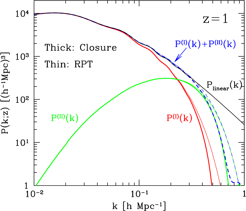
Refer to caption
Figure 2.— Power spectrum of density fluctuations P11(k;z)subscript𝑃11𝑘𝑧P_{11}(k;z) at z=1𝑧1z=1, obtained from the first-order Born approximation to the integral solution (see Eq.[68]). The contributions to the total power spectrum are separately plotted as indicated by P(I)(k)superscript𝑃I𝑘P^{\rm(I)}(k) and P(II)(k)superscript𝑃II𝑘P^{\rm(II)}(k) in the panel and the total power spectrum, P(I)(k)+P(II)(k)superscript𝑃I𝑘superscript𝑃II𝑘P^{\rm(I)}(k)+P^{\rm(II)}(k), is depicted as the dashed lines. Note that in evaluating the power spectrum, the approximate solutions for the non-linear propagators Gabapproxsuperscriptsubscript𝐺𝑎𝑏approxG_{ab}^{\rm approx} were used. Thick and thin lines indicate the results using the approximate solutions Gabapproxsuperscriptsubscript𝐺𝑎𝑏approxG_{ab}^{\rm approx} from the closure theory and RPT, respectively.

Figure 2 illustrates the overall behaviors of non-linear power spectrum of density fluctuations P(k;z)P11(k;z)𝑃𝑘𝑧subscript𝑃11𝑘𝑧P(k;z)\equiv P_{11}(k;z) given at z=1𝑧1z=1, based on the Born approximation (68). Here, the contributions to the total power spectrum up to the first-order Born approximation, i.e., P(I)(k)superscript𝑃I𝑘P^{\rm(I)}(k) and P(II)(k)superscript𝑃II𝑘P^{\rm(II)}(k), are separately plotted. Thin and thick lines represent the results from RPT and the closure theory, respectively. The result from RPT is basically the same one as presented by Crocce & Scoccimarro (2007), although they further considered the higher-order contribution coming from the two-loop correction. Due to the damping behavior in the non-linear propagators, each contribution to the total power spectrum rapidly falls off in both predictions and their amplitudes become significantly lower than the linear power spectrum on small scales (labeled by Plinear(k)subscript𝑃linear𝑘P_{\rm linear}(k)), where the differences between the two predictions become manifest. Turning to focus on the scales larger than the damping scale, the contribution coming from P(II)superscript𝑃IIP^{\rm(II)} becomes maximum around k0.2hMpc1similar-to𝑘0.2superscriptMpc1k\sim 0.2h\,\mbox{Mpc}^{-1}, where the non-linear enhancement of the power spectrum P(k)𝑃𝑘P(k) can be seen and the differences between closure theory and RPT become fairly small. In particular, for the scale of our interest on BAOs around k<0.010.3hMpc1superscriptsimilar-to𝑘0.010.3superscriptMpc1k\lower 2.15277pt\hbox{$\;\buildrel<\over{\sim}\;$}0.01-0.3h\,\mbox{Mpc}^{-1}, one cannot clearly distinguish between both predictions from Figure 2.
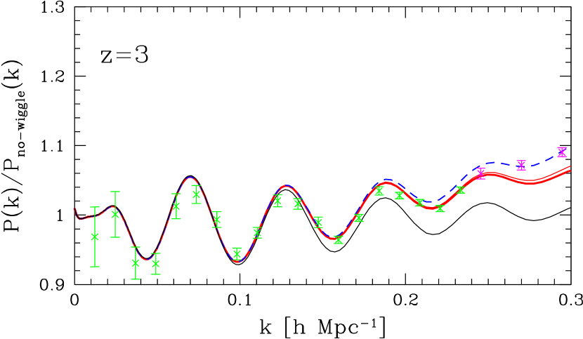
Refer to captionRefer to caption

Refer to captionRefer to caption

Figure 3.— Ratio of non-linear power spectrum to smoothed linear spectrum, P(k)/Pno-wiggle(k)𝑃𝑘subscript𝑃no-wiggle𝑘P(k)/P_{\rm no\mbox{-}wiggle}(k), given at specific redshifts, z=3𝑧3z=3, 222, 111 and 0.50.50.5. The error bar represents the N-body results taken from Jeong & Komatsu (2006), in which different color indicates the results with different box size (see their paper in detail). Here, smoothed linear spectra Pno-wiggle(k)subscript𝑃no-wiggle𝑘P_{\rm no\mbox{-}wiggle}(k) were calculated from the linear transfer function without baryon acoustic oscillation according to the fitting formula of Eisenstein & Hu (1998) (Eq.[29] of their paper). The non-linear power spectra are obtained from the first-order Born approximation to the integral solution (Eq.[68]), with approximate solutions of the non-linear propagator given by closure theory (thick) and RPT (thin). For comparison, one-loop predictions from the standard perturbation theory are plotted in dashed lines. Also, in panels with z=1𝑧1z=1 and 0.50.50.5, maximum wave number for limitation of one-loop perturbation is indicated by vertical arrows, according to the criterion, Δ2(k)k3P(k)/(2π2)<0.4superscriptΔ2𝑘superscript𝑘3𝑃𝑘2superscript𝜋2superscriptsimilar-to0.4\Delta^{2}(k)\equiv k^{3}P(k)/(2\pi^{2})\lower 2.15277pt\hbox{$\;\buildrel<\over{\sim}\;$}0.4 (Jeong & Komatsu, 2006).

To enlarge the differences between the two predictions and to clarify the non-linear behaviors of the BAOs, in Figure 3, snapshots of the power spectra divided by the smooth linear spectrum, P(k)/Pno-wiggle(k)𝑃𝑘subscript𝑃no-wiggle𝑘P(k)/P_{\rm no\mbox{-}wiggle}(k) are plotted for specific redshifts z=3𝑧3z=3, 222, 111 and 0.50.50.5 together with the N𝑁N-body results kindly provided by Jeong & Komatsu (2006) (except for z=0.5), while in Figure 4, we present the logarithmic derivative of the power spectra, dlnP(k)/dlnk𝑑𝑃𝑘𝑑𝑘d\ln P(k)/d\ln k. All the results are plotted in linear scales. The smooth power spectra, Pno-wiggle(k)subscript𝑃no-wiggle𝑘P_{\rm no\mbox{-}wiggle}(k), was calculated from the linear transfer function without BAOs based on the fitting formula of Eisenstein & Hu (1998) (see Eq.[29] in their paper). Note that the power spectra calculated from the closure theory and RPT are the sum of the leading-order contributions, P(I)(k)superscript𝑃I𝑘P^{\rm(I)}(k) and P(II)(k)superscript𝑃II𝑘P^{\rm(II)}(k), not including the higher-order term P(III)(k)superscript𝑃III𝑘P^{\rm(III)}(k). For comparison, the one-loop predictions from the standard perturbation theory are also depicted as dashed lines.

On large scales (low-k𝑘k), the predictions both from the closure theory and RPT reasonably match the one-loop results of standard perturbation theory, as anticipated. This is just the quantitative check for the non-perturbative methods discussed in section 4.1. On the other hand, on smaller scales (high-k𝑘k), the deviations from the one-loop perturbation become manifest and the amplitude of the predictions both from closure theory and RPT is suppressed compared to the one-loop predictions. The reduction of the power spectrum amplitude is the natural outcome of the damping behaviors appearing in the non-linear propagator and it qualitatively explains the behaviors seen in the N-body simulations (e.g., Jeong & Komatsu, 2006; Matarrese & Pietroni, 2007; Crocce & Scoccimarro, 2007). However, at lower redshifts z=1𝑧1z=1 and z=0.5𝑧0.5z=0.5, the suppression of the amplitude is so significant that the predictions eventually become lower than the linear theory prediction. Compared to the prediction from RPT, the suppression of the amplitude is even larger for the prediction from the closure theory.
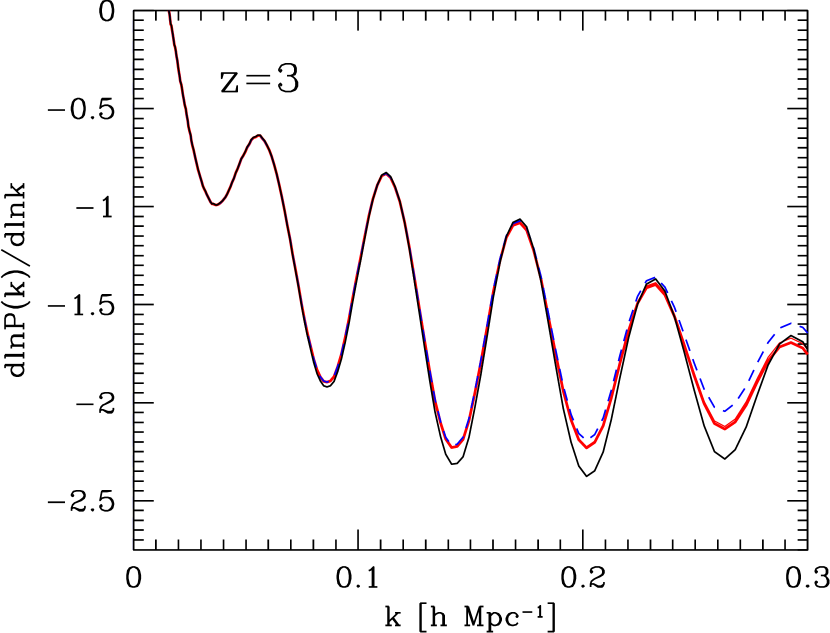
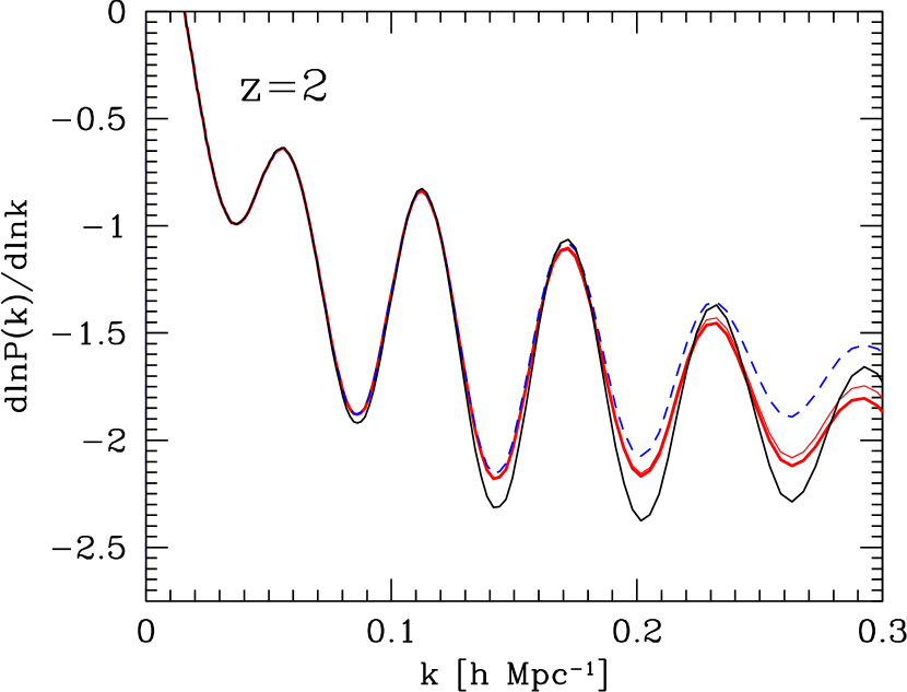
Refer to captionRefer to caption

Refer to captionRefer to caption

Figure 4.— Logarithmic derivative of non-linear power spectrum, dlnP(k)/dlnk𝑑𝑃𝑘𝑑𝑘d\ln P(k)/d\ln k, at redshifts z=3𝑧3z=3, 222, 111 and 0.50.50.5. Line types and labels are the same as in Fig.3.

The strong suppression seen in the low redshifts seems somewhat unphysical, indicating the failure of our present analysis. In the panels with redshift z=1𝑧1z=1 and z=0.5𝑧0.5z=0.5 of Figures 3 and 4, the maximum wave number for the limitation of one-loop perturbation theory is estimated according to the condition, Δ2(k)k3P(k)/(2π2)<0.4superscriptΔ2𝑘superscript𝑘3𝑃𝑘2superscript𝜋2superscriptsimilar-to0.4\Delta^{2}(k)\equiv k^{3}P(k)/(2\pi^{2})\lower 2.15277pt\hbox{$\;\buildrel<\over{\sim}\;$}0.4, given by Jeong & Komatsu (2006) and is depicted as vertical arrows, above which the perturbation prediction fails to reproduce the N-body results within the 1%percent11\% accuracy. Comparaed to those critical scales, the validity range of the non-perturbative predictions seems rather narrow. While this statement seems rather controversial, our present analysis actually relies on several approximate treatments. Hence, the inclusion of the higher-order terms such as P(III)(k)superscript𝑃III𝑘P^{\rm(III)}(k) might be essential for the correct non-linear behaviors. Crocce & Scoccimarro (2007) reported that the contributions higher than the two-loop correction become important on small scales and the prediction including the two-loop correction does improve the prediction, which reasonably agrees with N-body results within an accuracy of the N-body calculation. As we noted previously, however, the two-loop correction evaluated by the first-order Born approximation is comparable to the higher-order Born approximation coming from the P(III)(k)superscript𝑃III𝑘P^{\rm(III)}(k) term, and at a level of the present analysis, it is not clear whether the higher-loop corrections rather than the higher-order Born approximation of the one-loop correction are essential or not. Rather, one obvious thing is that a further improvement of the approximate treatment is necessary to faithfully predict the non-linear evolution of BAOs. In the line of this, self-consistent treatment to solve the evolution equations (53), (54) and (55), would be one plausible approach, which we will address this issue in next task.

6. Conclusions

In this paper, motivated by a forthcoming experiment on the precision measurement of the BAOs imprinted on the matter power spectrum, a new theoretical tool for predicting the non-linear gravitational evolution of power spectrum was presented. In particular, we have applied the non-linear statistical method in turbulence to the cosmological perturbation theory and derived a closed set of matter power spectrum. The resultant evolution equations (53)–(55) with Fourier kernels (56) and (57) are the non-linear coupled system of integro-differential equations and these consistently recover the one-loop results of standard perturbation theory. Further, the exact integral expressions for the solutions of closure equations were obtained (see Eqs.[64] and [65] with mode-coupling function [66]), whose analytical expressions coincide with the renormalized one-loop results of the theory developed by Crocce & Scoccimarro (2006a), apart from the corrections coming from the vertex renormalization.

Based on the Born approximation to the exact integral expressions, we next tried to evaluate the non-linear power spectrum analytically. Constructing an approximate solution for non-linear propagator, which smoothly matches the two asymptotic solutions valid at low-k𝑘k and high-k𝑘k, power spectrum of density fluctuations was computed and the results are compared with those obtained from the RPT. Due to the non-linear damping behavior of the non-linear propagator, the resultant amplitude of the power spectra up to the first-order Born approximation is strongly suppressed on small scales and this effect becomes significant as decreasing redshift. As a result, predicted spectra at high-k𝑘k both from the closure theory and RPT fail to reproduce the N-body trends and the inclusion of the higher-order corrections is required. Nevertheless, at the intermediate scales, where the damping behavior of the non-linear propagator is rather mild, the closure theory and RPT both predict the deviation from the one-loop results of standard perturbation theory, which qualitatively agree with the N-body results.

Although the analytical treatment presented here is still primitive and the range of the applicability is severely restricted by the validity of the approximations, the results indicate that our closure theory is a promising non-perturbative approach comparable to the RPT and a more elaborated study will provide an accurate prediction for non-linear power spectra going beyond standard perturbation theory. In this respect, a direct numerical treatment of the closure equations (53)–(55) is our urgent task. As it has been reported by Valageas (2007a), thanks to the full numerical treatment, the evolved result of the power spectrum shows several desirable properties and it qualitatively matches the N-body trends even at high-k𝑘k. In future publication, these points will be further investigated from a quantitative point-of-view, particularly focusing on the non-linear evolution of BAOs.

Finally, one criticism on the present approach including the currently existing non-perturbative methods is that the present methodology heavily relies on the single-stream approximation of the Vlasov equation. In a strongly non-linear regime at the high-k𝑘k region, the shell-crossing eventually occurs and the fluid description would be broken. A preliminary investigation suggests that the break down of the single-stream approximation may arise at k12hMpc1similar-to𝑘12superscriptMpc1k\sim 1-2\,h\mbox{Mpc}^{-1} (Scoccimarro, 2000; Afshordi, 2007). Therefore, for the high-k𝑘k region beyond the critical scale, the present approach cannot be applied and a more delicate treatment based on the Vlasov equation must be developed. This issue would be particularly crucial for accurate theoretical predictions to the cosmic shear statistics.


We are grateful to Keisuke Izumi, Shun Saito, Misao Sasaki, Jiro Soda and Yasushi Suto for useful discussions. We also thank Eiichiro Komatsu for providing the N-body data of Jeong & Komatsu (2006). This work is supported in part by a Grant-in-Aid for Scientific Research from the Japan Society for Promotion of Science (No. 18740132).

Appendix A One-loop perturbation

Here, we show that linear plus one-loop power spectra, Pab(11)(k)+Pab(22)(k)+Pab(13)(k)superscriptsubscript𝑃𝑎𝑏11𝑘superscriptsubscript𝑃𝑎𝑏22𝑘superscriptsubscript𝑃𝑎𝑏13𝑘P_{ab}^{(11)}(k)+P_{ab}^{(22)}(k)+P_{ab}^{(13)}(k), obtained from the standard perturbation theory indeed satisfy the evolution equations given by (61). To do this, we first write down the evolution equations for perturbed quantities Φa(i)(k;η)superscriptsubscriptΦ𝑎𝑖𝑘𝜂\Phi_{a}^{(i)}(k;\eta) in each order:

𝚲^ab(η)Φb(1)(𝒌;η)subscript^𝚲𝑎𝑏𝜂superscriptsubscriptΦ𝑏1𝒌𝜂\displaystyle\widehat{\mbox{\boldmath$\Lambda$}}_{ab}(\eta)\Phi_{b}^{(1)}(\mbox{\boldmath$k$};\eta) =\displaystyle= 0,0\displaystyle 0, (A1)
𝚲^ab(η)Φb(2)(𝒌;η)subscript^𝚲𝑎𝑏𝜂superscriptsubscriptΦ𝑏2𝒌𝜂\displaystyle\widehat{\mbox{\boldmath$\Lambda$}}_{ab}(\eta)\Phi_{b}^{(2)}(\mbox{\boldmath$k$};\eta) =\displaystyle= d3𝒌1d3𝒌2(2π)3δD(𝒌𝒌1𝒌2)γapq(𝒌1,𝒌2)Φp(1)(𝒌1;η)Φq(1)(𝒌2;η),superscript𝑑3subscript𝒌1superscript𝑑3subscript𝒌2superscript2𝜋3subscript𝛿𝐷𝒌subscript𝒌1subscript𝒌2subscript𝛾𝑎𝑝𝑞subscript𝒌1subscript𝒌2superscriptsubscriptΦ𝑝1subscript𝒌1𝜂superscriptsubscriptΦ𝑞1subscript𝒌2𝜂\displaystyle\int\frac{d^{3}\mbox{\boldmath$k$}_{1}d^{3}\mbox{\boldmath$k$}_{2}}{(2\pi)^{3}}\,\delta_{D}(\mbox{\boldmath$k$}-\mbox{\boldmath$k$}_{1}-\mbox{\boldmath$k$}_{2})\,\gamma_{apq}(\mbox{\boldmath$k$}_{1},\mbox{\boldmath$k$}_{2})\,\Phi_{p}^{(1)}(\mbox{\boldmath$k$}_{1};\eta)\Phi_{q}^{(1)}(\mbox{\boldmath$k$}_{2};\eta), (A2)
𝚲^ab(η)Φb(3)(𝒌;η)subscript^𝚲𝑎𝑏𝜂superscriptsubscriptΦ𝑏3𝒌𝜂\displaystyle\widehat{\mbox{\boldmath$\Lambda$}}_{ab}(\eta)\Phi_{b}^{(3)}(\mbox{\boldmath$k$};\eta) =\displaystyle= 2d3𝒌1d3𝒌2(2π)3δD(𝒌𝒌1𝒌2)γapq(𝒌1,𝒌2)Φp(1)(𝒌1;η)Φq(2)(𝒌2;η).2superscript𝑑3subscript𝒌1superscript𝑑3subscript𝒌2superscript2𝜋3subscript𝛿𝐷𝒌subscript𝒌1subscript𝒌2subscript𝛾𝑎𝑝𝑞subscript𝒌1subscript𝒌2superscriptsubscriptΦ𝑝1subscript𝒌1𝜂superscriptsubscriptΦ𝑞2subscript𝒌2𝜂\displaystyle 2\int\frac{d^{3}\mbox{\boldmath$k$}_{1}d^{3}\mbox{\boldmath$k$}_{2}}{(2\pi)^{3}}\,\delta_{D}(\mbox{\boldmath$k$}-\mbox{\boldmath$k$}_{1}-\mbox{\boldmath$k$}_{2})\,\gamma_{apq}(\mbox{\boldmath$k$}_{1},\mbox{\boldmath$k$}_{2})\,\Phi_{p}^{(1)}(\mbox{\boldmath$k$}_{1};\eta)\Phi_{q}^{(2)}(\mbox{\boldmath$k$}_{2};\eta). (A3)

The above equations are formally solved with a help of the linear propagator, gab(ηη)subscript𝑔𝑎𝑏𝜂superscript𝜂g_{ab}(\eta-\eta^{\prime}). For instance, the solution for second-order quantity Φa(2)superscriptsubscriptΦ𝑎2\Phi_{a}^{(2)} can be written as

Φa(2)(𝒌;η)superscriptsubscriptΦ𝑎2𝒌𝜂\displaystyle\Phi_{a}^{(2)}(\mbox{\boldmath$k$};\eta) =\displaystyle= η0η𝑑ηgab(ηη)superscriptsubscriptsubscript𝜂0𝜂differential-dsuperscript𝜂subscript𝑔𝑎𝑏𝜂superscript𝜂\displaystyle\int_{\eta_{0}}^{\eta}d\eta^{\prime}\,\,g_{ab}(\eta-\eta^{\prime})\, (A4)
×d3𝒌1d3𝒌2(2π)3δD(𝒌𝒌1𝒌2)γbpq(𝒌1,𝒌2)Φp(1)(𝒌1;η)Φq(1)(𝒌2;η).\displaystyle\times\int\frac{d^{3}\mbox{\boldmath$k$}_{1}d^{3}\mbox{\boldmath$k$}_{2}}{(2\pi)^{3}}\,\,\delta_{D}(\mbox{\boldmath$k$}-\mbox{\boldmath$k$}_{1}-\mbox{\boldmath$k$}_{2})\,\,\gamma_{bpq}(\mbox{\boldmath$k$}_{1},\mbox{\boldmath$k$}_{2})\,\Phi_{p}^{(1)}(\mbox{\boldmath$k$}_{1};\eta^{\prime})\Phi_{q}^{(1)}(\mbox{\boldmath$k$}_{2};\eta^{\prime}).

Now, let us consider the time evolution of power spectrum, P(22)(k;η)superscript𝑃22𝑘𝜂P^{(22)}(k;\eta). Acting the operator 𝚺^abcd(η)subscript^𝚺𝑎𝑏𝑐𝑑𝜂\widehat{\mathbf{\Sigma}}_{abcd}(\eta) defined by (24) on the ensemble average Φc(2)(𝒌;η)Φd(2)(𝒌;η)delimited-⟨⟩superscriptsubscriptΦ𝑐2𝒌𝜂superscriptsubscriptΦ𝑑2superscript𝒌𝜂\langle\Phi_{c}^{(2)}(\mbox{\boldmath$k$};\eta)\Phi_{d}^{(2)}(\mbox{\boldmath$k$}^{\prime};\eta)\rangle, we obtain

𝚺^abcd(η)Φc(2)(𝒌;η)Φd(2)(𝒌;η)subscript^𝚺𝑎𝑏𝑐𝑑𝜂delimited-⟨⟩superscriptsubscriptΦ𝑐2𝒌𝜂superscriptsubscriptΦ𝑑2superscript𝒌𝜂\displaystyle\widehat{\mathbf{\Sigma}}_{abcd}(\eta)\,\Bigl{\langle}\Phi_{c}^{(2)}(\mbox{\boldmath$k$};\eta)\Phi_{d}^{(2)}(\mbox{\boldmath$k$}^{\prime};\eta)\Bigr{\rangle}
=Φa(2)(𝒌;η){𝚲^bd(η)Φd(2)(𝒌;η)}+{𝚲^ac(η)Φc(2)(𝒌;η)}Φb(2)(𝒌;η)absentdelimited-⟨⟩superscriptsubscriptΦ𝑎2𝒌𝜂subscript^𝚲𝑏𝑑𝜂superscriptsubscriptΦ𝑑2superscript𝒌𝜂delimited-⟨⟩subscript^𝚲𝑎𝑐𝜂superscriptsubscriptΦ𝑐2𝒌𝜂superscriptsubscriptΦ𝑏2superscript𝒌𝜂\displaystyle\quad\quad=\Bigl{\langle}\Phi_{a}^{(2)}(\mbox{\boldmath$k$};\eta)\,\,\left\{\widehat{\mathbf{\Lambda}}_{bd}(\eta)\,\Phi_{d}^{(2)}(\mbox{\boldmath$k$}^{\prime};\eta)\right\}\Bigr{\rangle}+\Bigl{\langle}\left\{\widehat{\mathbf{\Lambda}}_{ac}(\eta)\,\Phi_{c}^{(2)}(\mbox{\boldmath$k$};\eta)\right\}\,\,\Phi_{b}^{(2)}(\mbox{\boldmath$k$}^{\prime};\eta)\Bigr{\rangle}
=η0η𝑑ηgal(ηη)d3𝒌1d3𝒌2(2π)3d3𝒌3d3𝒌4(2π)3δD(𝒌𝒌1𝒌2)δD(𝒌𝒌3𝒌4)absentsuperscriptsubscriptsubscript𝜂0𝜂differential-dsuperscript𝜂subscript𝑔𝑎𝑙𝜂superscript𝜂superscript𝑑3subscript𝒌1superscript𝑑3subscript𝒌2superscript2𝜋3superscript𝑑3subscript𝒌3superscript𝑑3subscript𝒌4superscript2𝜋3subscript𝛿𝐷𝒌subscript𝒌1subscript𝒌2subscript𝛿𝐷superscript𝒌subscript𝒌3subscript𝒌4\displaystyle\quad\quad=\int_{\eta_{0}}^{\eta}d\eta^{\prime}\,g_{al}(\eta-\eta^{\prime})\int\frac{d^{3}\mbox{\boldmath$k$}_{1}d^{3}\mbox{\boldmath$k$}_{2}}{(2\pi)^{3}}\int\frac{d^{3}\mbox{\boldmath$k$}_{3}d^{3}\mbox{\boldmath$k$}_{4}}{(2\pi)^{3}}\,\,\delta_{D}(\mbox{\boldmath$k$}-\mbox{\boldmath$k$}_{1}-\mbox{\boldmath$k$}_{2})\,\delta_{D}(\mbox{\boldmath$k$}^{\prime}-\mbox{\boldmath$k$}_{3}-\mbox{\boldmath$k$}_{4})\,
×γlrs(𝒌1,𝒌2)γbpq(𝒌3,𝒌4)Φr(1)(𝒌1;η)Φs(1)(𝒌2;η)Φp(1)(𝒌3;η)Φq(1)(𝒌4;η)absentsubscript𝛾𝑙𝑟𝑠subscript𝒌1subscript𝒌2subscript𝛾𝑏𝑝𝑞subscript𝒌3subscript𝒌4delimited-⟨⟩superscriptsubscriptΦ𝑟1subscript𝒌1superscript𝜂superscriptsubscriptΦ𝑠1subscript𝒌2superscript𝜂superscriptsubscriptΦ𝑝1subscript𝒌3𝜂superscriptsubscriptΦ𝑞1subscript𝒌4𝜂\displaystyle\quad\quad\quad\quad\times\,\gamma_{lrs}(\mbox{\boldmath$k$}_{1},\mbox{\boldmath$k$}_{2})\,\gamma_{bpq}(\mbox{\boldmath$k$}_{3},\mbox{\boldmath$k$}_{4})\,\Bigl{\langle}\Phi_{r}^{(1)}(\mbox{\boldmath$k$}_{1};\eta^{\prime})\Phi_{s}^{(1)}(\mbox{\boldmath$k$}_{2};\eta^{\prime})\Phi_{p}^{(1)}(\mbox{\boldmath$k$}_{3};\eta)\Phi_{q}^{(1)}(\mbox{\boldmath$k$}_{4};\eta)\Bigr{\rangle}
+(ab,𝒌𝒌),\displaystyle\quad\quad\quad+\quad\Bigl{(}\quad a\longleftrightarrow b,\quad\quad\mbox{\boldmath$k$}\longleftrightarrow\mbox{\boldmath$k$}^{\prime}\quad\Bigr{)},
=2η0η𝑑ηgal(ηη)d3𝒌1d3𝒌2δD(𝒌𝒌1𝒌2)δD(𝒌+𝒌1+𝒌2)absent2superscriptsubscriptsubscript𝜂0𝜂differential-dsuperscript𝜂subscript𝑔𝑎𝑙𝜂superscript𝜂superscript𝑑3subscript𝒌1superscript𝑑3subscript𝒌2subscript𝛿𝐷superscript𝒌subscript𝒌1subscript𝒌2subscript𝛿𝐷𝒌subscript𝒌1subscript𝒌2\displaystyle\quad\quad=2\int_{\eta_{0}}^{\eta}d\eta^{\prime}\,g_{al}(\eta-\eta^{\prime})\int d^{3}\mbox{\boldmath$k$}_{1}d^{3}\mbox{\boldmath$k$}_{2}\,\,\delta_{D}(\mbox{\boldmath$k$}^{\prime}-\mbox{\boldmath$k$}_{1}-\mbox{\boldmath$k$}_{2})\,\delta_{D}(\mbox{\boldmath$k$}+\mbox{\boldmath$k$}_{1}+\mbox{\boldmath$k$}_{2})\,
×γbpq(𝒌1,𝒌2)γlrs(𝒌1,𝒌2)Rpr(11)(k1;η,η)Rqs(11)(k2;η,η),absentsubscript𝛾𝑏𝑝𝑞subscript𝒌1subscript𝒌2subscript𝛾𝑙𝑟𝑠subscript𝒌1subscript𝒌2superscriptsubscript𝑅𝑝𝑟11subscript𝑘1𝜂superscript𝜂superscriptsubscript𝑅𝑞𝑠11subscript𝑘2𝜂superscript𝜂\displaystyle\quad\quad\quad\quad\times\,\gamma_{bpq}(\mbox{\boldmath$k$}_{1},\mbox{\boldmath$k$}_{2})\gamma_{lrs}(\mbox{\boldmath$k$}_{1},\mbox{\boldmath$k$}_{2})R_{pr}^{(11)}(k_{1};\eta,\eta^{\prime})R_{qs}^{(11)}(k_{2};\eta,\eta^{\prime}),
+(ab,𝒌𝒌),\displaystyle\quad\quad\quad+\quad\Bigl{(}\quad a\longleftrightarrow b,\quad\quad\mbox{\boldmath$k$}\longleftrightarrow\mbox{\boldmath$k$}^{\prime}\quad\Bigr{)}, (A5)

where, in the last equality, we have replaced the four-point functions with a product of the two-point functions Rab(11)superscriptsubscript𝑅𝑎𝑏11R_{ab}^{(11)} according to Wick’s theorem. The quantity Rab(11)superscriptsubscript𝑅𝑎𝑏11R_{ab}^{(11)} is the linear cross spectrum defined by

Φa(1)(𝒌;η)Φb(1)(𝒌;η)=(2π)3δD(𝒌+𝒌)Rab(11)(k;η,η),(ηη).delimited-⟨⟩superscriptsubscriptΦ𝑎1𝒌𝜂superscriptsubscriptΦ𝑏1superscript𝒌superscript𝜂superscript2𝜋3subscript𝛿𝐷𝒌superscript𝒌superscriptsubscript𝑅𝑎𝑏11𝑘𝜂superscript𝜂𝜂superscript𝜂\displaystyle\Bigl{\langle}\Phi_{a}^{(1)}(\mbox{\boldmath$k$};\eta)\Phi_{b}^{(1)}(\mbox{\boldmath$k$}^{\prime};\eta^{\prime})\Bigr{\rangle}=(2\pi)^{3}\,\delta_{D}(\mbox{\boldmath$k$}+\mbox{\boldmath$k$}^{\prime})\,\,R_{ab}^{(11)}(k;\eta,\eta^{\prime}),\quad(\eta\geq\eta^{\prime}). (A6)

Integrating equation (A5) over the Fourier mode 𝒌superscript𝒌\mbox{\boldmath$k$}^{\prime} leads to

𝚺^abcd(η)Pcd(22)(k;η)subscript^𝚺𝑎𝑏𝑐𝑑𝜂superscriptsubscript𝑃𝑐𝑑22𝑘𝜂\displaystyle\widehat{\mathbf{\Sigma}}_{abcd}(\eta)\,P_{cd}^{(22)}(k;\eta) =\displaystyle= 2η0η𝑑ηgal(ηη)d3𝒌1d3𝒌2(2π)3δD(𝒌+𝒌1+𝒌2)2superscriptsubscriptsubscript𝜂0𝜂differential-dsuperscript𝜂subscript𝑔𝑎𝑙𝜂superscript𝜂superscript𝑑3subscript𝒌1superscript𝑑3subscript𝒌2superscript2𝜋3subscript𝛿𝐷𝒌subscript𝒌1subscript𝒌2\displaystyle 2\int_{\eta_{0}}^{\eta}d\eta^{\prime}\,g_{al}(\eta-\eta^{\prime})\int\frac{d^{3}\mbox{\boldmath$k$}_{1}d^{3}\mbox{\boldmath$k$}_{2}}{(2\pi)^{3}}\,\,\delta_{D}(\mbox{\boldmath$k$}+\mbox{\boldmath$k$}_{1}+\mbox{\boldmath$k$}_{2})\,\, (A7)
×γlrs(𝒌1,𝒌2)γbpq(𝒌1,𝒌2)Rpr(11)(k1;η,η)Rqs(11)(k2;η,η)absentsubscript𝛾𝑙𝑟𝑠subscript𝒌1subscript𝒌2subscript𝛾𝑏𝑝𝑞subscript𝒌1subscript𝒌2superscriptsubscript𝑅𝑝𝑟11subscript𝑘1𝜂superscript𝜂superscriptsubscript𝑅𝑞𝑠11subscript𝑘2𝜂superscript𝜂\displaystyle\quad\quad\quad\times\,\gamma_{lrs}(\mbox{\boldmath$k$}_{1},\mbox{\boldmath$k$}_{2})\,\gamma_{bpq}(\mbox{\boldmath$k$}_{1},\mbox{\boldmath$k$}_{2})\,R_{pr}^{(11)}(k_{1};\eta,\eta^{\prime})R_{qs}^{(11)}(k_{2};\eta,\eta^{\prime})
+\displaystyle+ (ab,𝒌𝒌).\displaystyle\quad\Bigl{(}\quad a\longleftrightarrow b,\quad\quad\mbox{\boldmath$k$}\longleftrightarrow-\mbox{\boldmath$k$}\quad\Bigr{)}.

Next consider the evolution equation for power spectrum P(13)(k;η)superscript𝑃13𝑘𝜂P^{(13)}(k;\eta). Repeating the similar calculations given above, we have

𝚺^abcd(η)Φc(1)(𝒌;η)Φd(3)(𝒌;η)+Φc(3)(𝒌;η)Φd(1)(𝒌;η)subscript^𝚺𝑎𝑏𝑐𝑑𝜂delimited-⟨⟩superscriptsubscriptΦ𝑐1𝒌𝜂superscriptsubscriptΦ𝑑3superscript𝒌𝜂superscriptsubscriptΦ𝑐3𝒌𝜂superscriptsubscriptΦ𝑑1superscript𝒌𝜂\displaystyle\widehat{\mathbf{\Sigma}}_{abcd}(\eta)\,\Bigl{\langle}\Phi_{c}^{(1)}(\mbox{\boldmath$k$};\eta)\Phi_{d}^{(3)}(\mbox{\boldmath$k$}^{\prime};\eta)+\Phi_{c}^{(3)}(\mbox{\boldmath$k$};\eta)\Phi_{d}^{(1)}(\mbox{\boldmath$k$}^{\prime};\eta)\Bigr{\rangle}
=Φa(1)(𝒌;η){𝚲^bd(η)Φd(3)(𝒌;η)}+{𝚲^ac(η)Φc(3)(𝒌;η)}Φb(1)(𝒌;η)absentdelimited-⟨⟩superscriptsubscriptΦ𝑎1𝒌𝜂subscript^𝚲𝑏𝑑𝜂superscriptsubscriptΦ𝑑3superscript𝒌𝜂delimited-⟨⟩subscript^𝚲𝑎𝑐𝜂superscriptsubscriptΦ𝑐3𝒌𝜂superscriptsubscriptΦ𝑏1superscript𝒌𝜂\displaystyle\quad\quad=\Bigl{\langle}\Phi_{a}^{(1)}(\mbox{\boldmath$k$};\eta)\,\,\left\{\widehat{\mathbf{\Lambda}}_{bd}(\eta)\,\Phi_{d}^{(3)}(\mbox{\boldmath$k$}^{\prime};\eta)\right\}\Bigr{\rangle}+\Bigl{\langle}\left\{\widehat{\mathbf{\Lambda}}_{ac}(\eta)\,\Phi_{c}^{(3)}(\mbox{\boldmath$k$};\eta)\right\}\,\,\Phi_{b}^{(1)}(\mbox{\boldmath$k$}^{\prime};\eta)\Bigr{\rangle}
=2η0η𝑑ηd3𝒌1d3𝒌2(2π)3d3𝒌3d3𝒌4(2π)3δD(𝒌𝒌1𝒌2)δD(𝒌2𝒌3𝒌4)absent2superscriptsubscriptsubscript𝜂0𝜂differential-dsuperscript𝜂superscript𝑑3subscript𝒌1superscript𝑑3subscript𝒌2superscript2𝜋3superscript𝑑3subscript𝒌3superscript𝑑3subscript𝒌4superscript2𝜋3subscript𝛿𝐷superscript𝒌subscript𝒌1subscript𝒌2subscript𝛿𝐷subscript𝒌2subscript𝒌3subscript𝒌4\displaystyle\quad\quad=2\int_{\eta_{0}}^{\eta}d\eta^{\prime}\int\frac{d^{3}\mbox{\boldmath$k$}_{1}d^{3}\mbox{\boldmath$k$}_{2}}{(2\pi)^{3}}\int\frac{d^{3}\mbox{\boldmath$k$}_{3}d^{3}\mbox{\boldmath$k$}_{4}}{(2\pi)^{3}}\,\,\delta_{D}(\mbox{\boldmath$k$}^{\prime}-\mbox{\boldmath$k$}_{1}-\mbox{\boldmath$k$}_{2})\,\delta_{D}(\mbox{\boldmath$k$}_{2}-\mbox{\boldmath$k$}_{3}-\mbox{\boldmath$k$}_{4})
×gql(ηη)γbpq(𝒌1,𝒌2)γlrs(𝒌3,𝒌4)Φa(1)(𝒌;η)Φp(1)(𝒌1;η)Φr(1)(𝒌3;η)Φs(1)(𝒌4;η)absentsubscript𝑔𝑞𝑙𝜂superscript𝜂subscript𝛾𝑏𝑝𝑞subscript𝒌1subscript𝒌2subscript𝛾𝑙𝑟𝑠subscript𝒌3subscript𝒌4delimited-⟨⟩superscriptsubscriptΦ𝑎1𝒌𝜂superscriptsubscriptΦ𝑝1subscript𝒌1𝜂superscriptsubscriptΦ𝑟1subscript𝒌3superscript𝜂superscriptsubscriptΦ𝑠1subscript𝒌4superscript𝜂\displaystyle\quad\quad\quad\quad\times\,g_{ql}(\eta-\eta^{\prime})\,\gamma_{bpq}(\mbox{\boldmath$k$}_{1},\mbox{\boldmath$k$}_{2})\,\gamma_{lrs}(\mbox{\boldmath$k$}_{3},\mbox{\boldmath$k$}_{4})\Bigl{\langle}\Phi_{a}^{(1)}(\mbox{\boldmath$k$};\eta)\Phi_{p}^{(1)}(\mbox{\boldmath$k$}_{1};\eta)\Phi_{r}^{(1)}(\mbox{\boldmath$k$}_{3};\eta^{\prime})\Phi_{s}^{(1)}(\mbox{\boldmath$k$}_{4};\eta^{\prime})\Bigr{\rangle}
+(ab,𝒌𝒌)\displaystyle\quad\quad\quad\quad+\quad\Bigl{(}\quad a\longleftrightarrow b,\quad\quad\mbox{\boldmath$k$}\longleftrightarrow\mbox{\boldmath$k$}^{\prime}\quad\Bigr{)}
=4η0η𝑑ηgql(ηη)d3𝒌1d3𝒌2δD(𝒌𝒌1𝒌2)δD(𝒌+𝒌1+𝒌2)absent4superscriptsubscriptsubscript𝜂0𝜂differential-dsuperscript𝜂subscript𝑔𝑞𝑙𝜂superscript𝜂superscript𝑑3subscript𝒌1superscript𝑑3subscript𝒌2subscript𝛿𝐷superscript𝒌subscript𝒌1subscript𝒌2subscript𝛿𝐷𝒌subscript𝒌1subscript𝒌2\displaystyle\quad\quad=4\int_{\eta_{0}}^{\eta}d\eta^{\prime}\,g_{ql}(\eta-\eta^{\prime})\int d^{3}\mbox{\boldmath$k$}_{1}d^{3}\mbox{\boldmath$k$}_{2}\,\,\delta_{D}(\mbox{\boldmath$k$}^{\prime}-\mbox{\boldmath$k$}_{1}-\mbox{\boldmath$k$}_{2})\,\delta_{D}(\mbox{\boldmath$k$}+\mbox{\boldmath$k$}_{1}+\mbox{\boldmath$k$}_{2})\,
×γbpq(𝒌1,𝒌2)γlrs(𝒌,𝒌1)Rar(11)(k;η,η)Rps(11)(k1;η,η)absentsubscript𝛾𝑏𝑝𝑞subscript𝒌1subscript𝒌2subscript𝛾𝑙𝑟𝑠𝒌subscript𝒌1superscriptsubscript𝑅𝑎𝑟11𝑘𝜂superscript𝜂superscriptsubscript𝑅𝑝𝑠11subscript𝑘1𝜂superscript𝜂\displaystyle\quad\quad\quad\quad\times\,\gamma_{bpq}(\mbox{\boldmath$k$}_{1},\mbox{\boldmath$k$}_{2})\gamma_{lrs}(\mbox{\boldmath$k$},\mbox{\boldmath$k$}_{1})R_{ar}^{(11)}(k;\eta,\eta^{\prime})R_{ps}^{(11)}(k_{1};\eta,\eta^{\prime})
+(ab,𝒌𝒌).\displaystyle\quad\quad\quad+\quad\Bigl{(}\quad a\longleftrightarrow b,\quad\quad\mbox{\boldmath$k$}\longleftrightarrow\mbox{\boldmath$k$}^{\prime}\quad\Bigr{)}.

Here, in the second equality of the above equation, we have used equations (A1) and (A3), and substituted the formal solution (A4) to rewrite all the perturbed quantities with the linear-order one, Φb(1)(𝐤,η)superscriptsubscriptΦ𝑏1𝐤𝜂\Phi_{b}^{(1)}(\mathbf{k},\eta). Then, integrating over 𝒌superscript𝒌\mbox{\boldmath$k$}^{\prime}, we obtain

𝚺^abcdPcd(13)(k;η)subscript^𝚺𝑎𝑏𝑐𝑑superscriptsubscript𝑃𝑐𝑑13𝑘𝜂\displaystyle\widehat{\mathbf{\Sigma}}_{abcd}P_{cd}^{(13)}(k;\eta) =\displaystyle= 4η0η𝑑ηgql(ηη)d3𝒌1d3𝒌2(2π)3δD(𝒌+𝒌1+𝒌2)4superscriptsubscriptsubscript𝜂0𝜂differential-dsuperscript𝜂subscript𝑔𝑞𝑙𝜂superscript𝜂superscript𝑑3subscript𝒌1superscript𝑑3subscript𝒌2superscript2𝜋3subscript𝛿𝐷𝒌subscript𝒌1subscript𝒌2\displaystyle 4\int_{\eta_{0}}^{\eta}d\eta^{\prime}\,g_{ql}(\eta-\eta^{\prime})\,\int\frac{d^{3}\mbox{\boldmath$k$}_{1}d^{3}\mbox{\boldmath$k$}_{2}}{(2\pi)^{3}}\,\,\delta_{D}(\mbox{\boldmath$k$}+\mbox{\boldmath$k$}_{1}+\mbox{\boldmath$k$}_{2})\,\, (A8)
×γbpq(𝒌1,𝒌2)γlrs(𝒌,𝒌1)Rar(11)(k;η,η)Rps(11)(k1;η,η)absentsubscript𝛾𝑏𝑝𝑞subscript𝒌1subscript𝒌2subscript𝛾𝑙𝑟𝑠𝒌subscript𝒌1superscriptsubscript𝑅𝑎𝑟11𝑘𝜂superscript𝜂superscriptsubscript𝑅𝑝𝑠11subscript𝑘1𝜂superscript𝜂\displaystyle\quad\quad\quad\times\,\,\gamma_{bpq}(\mbox{\boldmath$k$}_{1},\mbox{\boldmath$k$}_{2})\,\gamma_{lrs}(\mbox{\boldmath$k$},\mbox{\boldmath$k$}_{1})\,R_{ar}^{(11)}(k;\eta,\eta^{\prime})R_{ps}^{(11)}(k_{1};\eta,\eta^{\prime})
+(ab,𝒌𝒌).\displaystyle\quad+\quad\Bigl{(}\quad a\longleftrightarrow b,\quad\quad\mbox{\boldmath$k$}\longleftrightarrow-\mbox{\boldmath$k$}\quad\Bigr{)}.

Summing up equations (A7) and (A8), and using the fact that 𝚺^abcd(η)Pcd(11)(k;η)=0subscript^𝚺𝑎𝑏𝑐𝑑𝜂superscriptsubscript𝑃𝑐𝑑11𝑘𝜂0\widehat{\mathbf{\Sigma}}_{abcd}(\eta)\,P_{cd}^{(11)}(k;\eta)=0, we finally arrive at equation (61).

Appendix B Integral solutions

In this appendix, we show that the integral expressions given in Section 4.2 are compatible with the closure equations (53) and (54). Here, we shall particularly focus on the integral expression (65) and explicitly derive the closure equation (54) from equation (65). As for the integral expression (64), it is straightforward to show the compatibility between equations (53) and (64), just repeating the same procedure as presented below.

Let us consider equation (65) and separate the right-hand side of this equation into two terms:

Rbc(I)(k;η,η)superscriptsubscript𝑅𝑏𝑐I𝑘𝜂superscript𝜂\displaystyle R_{bc}^{\rm(I)}(k;\eta,\eta^{\prime}) =\displaystyle= Gbd(k|η,η0)Gce(k|η,η0)Pde(k;η0),subscript𝐺𝑏𝑑conditional𝑘𝜂subscript𝜂0subscript𝐺𝑐𝑒conditional𝑘superscript𝜂subscript𝜂0subscript𝑃𝑑𝑒𝑘subscript𝜂0\displaystyle G_{bd}(k|\eta,\eta_{0})\,G_{ce}(k|\eta^{\prime},\eta_{0})\,P_{de}(k;\eta_{0}),
Rbc(II)(k;η,η)superscriptsubscript𝑅𝑏𝑐II𝑘𝜂superscript𝜂\displaystyle R_{bc}^{\rm(II)}(k;\eta,\eta^{\prime}) =\displaystyle= η0η𝑑η1η0η𝑑η2Gbd(k|η,η1)Gce(k|η,η2)Φde(k;η2,η1).superscriptsubscriptsubscript𝜂0𝜂differential-dsubscript𝜂1superscriptsubscriptsubscript𝜂0superscript𝜂differential-dsubscript𝜂2subscript𝐺𝑏𝑑conditional𝑘𝜂subscript𝜂1subscript𝐺𝑐𝑒conditional𝑘superscript𝜂subscript𝜂2subscriptΦ𝑑𝑒𝑘subscript𝜂2subscript𝜂1\displaystyle\int_{\eta_{0}}^{\eta}d\eta_{1}\int_{\eta_{0}}^{\eta^{\prime}}d\eta_{2}\,\,G_{bd}(k|\eta,\eta_{1})\,G_{ce}(k|\eta^{\prime},\eta_{2})\,\Phi_{de}(k;\eta_{2},\eta_{1}).

Acting the operator 𝚲^ab(η)subscript^𝚲𝑎𝑏𝜂\widehat{\mbox{\boldmath$\Lambda$}}_{ab}(\eta) on the above equations, with a help of equation (55), we have

𝚲^ab(η)Rbc(I)(k;η,η)=4η0η𝑑η1d3𝒒(2π)3γapq(𝒒,𝒌𝒒)γlrs(𝒒,𝒌)subscript^𝚲𝑎𝑏𝜂superscriptsubscript𝑅𝑏𝑐I𝑘𝜂superscript𝜂4superscriptsubscriptsubscript𝜂0𝜂differential-dsubscript𝜂1superscript𝑑3𝒒superscript2𝜋3subscript𝛾𝑎𝑝𝑞𝒒𝒌𝒒subscript𝛾𝑙𝑟𝑠𝒒𝒌\displaystyle\widehat{\mathbf{\Lambda}}_{ab}(\eta)\,\,R_{bc}^{\rm(I)}(k;\eta,\eta^{\prime})=4\int_{\eta_{0}}^{\eta}d\eta_{1}\int\frac{d^{3}\mbox{\boldmath$q$}}{(2\pi)^{3}}\,\gamma_{apq}(\mbox{\boldmath$q$},\mbox{\boldmath$k$}-\mbox{\boldmath$q$})\,\gamma_{lrs}(-\mbox{\boldmath$q$},\mbox{\boldmath$k$})
×Gql(|𝒌𝒒||η,η1)Rpr(q;η,η1)Gsb(k|η1,η0)Gcd(k|η,η0)Pbd(k;η0),absentsubscript𝐺𝑞𝑙conditional𝒌𝒒𝜂subscript𝜂1subscript𝑅𝑝𝑟𝑞𝜂subscript𝜂1subscript𝐺𝑠𝑏conditional𝑘subscript𝜂1subscript𝜂0subscript𝐺𝑐𝑑conditional𝑘superscript𝜂subscript𝜂0subscript𝑃𝑏𝑑𝑘subscript𝜂0\displaystyle\quad\quad\quad\quad\quad\times\,\,G_{ql}(|\mbox{\boldmath$k$}-\mbox{\boldmath$q$}||\eta,\eta_{1})\,R_{pr}(q;\eta,\eta_{1})\,G_{sb}(k|\eta_{1},\eta_{0})\,G_{cd}(k|\eta^{\prime},\eta_{0})\,P_{bd}(k;\eta_{0}),
𝚲^ab(η)Rbc(II)(k;η,η)=η0η𝑑η2Gce(k|η,η2)Φae(k;η2,η)subscript^𝚲𝑎𝑏𝜂superscriptsubscript𝑅𝑏𝑐II𝑘𝜂superscript𝜂superscriptsubscriptsubscript𝜂0superscript𝜂differential-dsubscript𝜂2subscript𝐺𝑐𝑒conditional𝑘superscript𝜂subscript𝜂2subscriptΦ𝑎𝑒𝑘subscript𝜂2𝜂\displaystyle\widehat{\mathbf{\Lambda}}_{ab}(\eta)\,\,R_{bc}^{\rm(II)}(k;\eta,\eta^{\prime})=\int_{\eta_{0}}^{\eta^{\prime}}d\eta_{2}\,\,G_{ce}(k|\eta^{\prime},\eta_{2})\,\Phi_{ae}(k;\eta_{2},\eta)
+  4η0η𝑑η1η0η𝑑η2η1η𝑑η3d3𝒒(2π)3γapq(𝒒,𝒌𝒒)γlrs(𝒒,𝒌),4superscriptsubscriptsubscript𝜂0𝜂differential-dsubscript𝜂1superscriptsubscriptsubscript𝜂0superscript𝜂differential-dsubscript𝜂2superscriptsubscriptsubscript𝜂1𝜂differential-dsubscript𝜂3superscript𝑑3𝒒superscript2𝜋3subscript𝛾𝑎𝑝𝑞𝒒𝒌𝒒subscript𝛾𝑙𝑟𝑠𝒒𝒌\displaystyle\quad\quad+\,\,4\int_{\eta_{0}}^{\eta}d\eta_{1}\int_{\eta_{0}}^{\eta^{\prime}}d\eta_{2}\int_{\eta_{1}}^{\eta}d\eta_{3}\int\frac{d^{3}\mbox{\boldmath$q$}}{(2\pi)^{3}}\,\,\gamma_{apq}(\mbox{\boldmath$q$},\mbox{\boldmath$k$}-\mbox{\boldmath$q$})\,\gamma_{lrs}(-\mbox{\boldmath$q$},\mbox{\boldmath$k$}),
×Gce(k|η,η2)Φde(k;η2,η1)Gql(|𝒌𝒒||η,η3)Rpr(q;η,η3)Gsd(k|η3,η1).absentsubscript𝐺𝑐𝑒conditional𝑘superscript𝜂subscript𝜂2subscriptΦ𝑑𝑒𝑘subscript𝜂2subscript𝜂1subscript𝐺𝑞𝑙conditional𝒌𝒒𝜂subscript𝜂3subscript𝑅𝑝𝑟𝑞𝜂subscript𝜂3subscript𝐺𝑠𝑑conditional𝑘subscript𝜂3subscript𝜂1\displaystyle\quad\quad\quad\quad\times\,\,G_{ce}(k|\eta^{\prime},\eta_{2})\,\Phi_{de}(k;\eta_{2},\eta_{1})\,G_{ql}(|\mbox{\boldmath$k$}-\mbox{\boldmath$q$}||\eta,\eta_{3})\,R_{pr}(q;\eta,\eta_{3})\,G_{sd}(k|\eta_{3},\eta_{1}).

Summing up the above two equations, we obtain

𝚲^ab(η){Rbc(I)+Rbc(II)}subscript^𝚲𝑎𝑏𝜂superscriptsubscript𝑅𝑏𝑐Isuperscriptsubscript𝑅𝑏𝑐II\displaystyle\widehat{\mathbf{\Lambda}}_{ab}(\eta)\,\,\left\{\,R_{bc}^{\rm(I)}+R_{bc}^{\rm(II)}\right\} =\displaystyle= η0η𝑑η2Gce(k|η,η2)Φae(k;η2,η)superscriptsubscriptsubscript𝜂0superscript𝜂differential-dsubscript𝜂2subscript𝐺𝑐𝑒conditional𝑘superscript𝜂subscript𝜂2subscriptΦ𝑎𝑒𝑘subscript𝜂2𝜂\displaystyle\int_{\eta_{0}}^{\eta^{\prime}}d\eta_{2}\,\,G_{ce}(k|\eta^{\prime},\eta_{2})\,\Phi_{ae}(k;\eta_{2},\eta) (B1)
+ 4d3𝒒(2π)3γapq(𝒒,𝒌𝒒)γlrs(𝒒,𝒌)[],4superscript𝑑3𝒒superscript2𝜋3subscript𝛾𝑎𝑝𝑞𝒒𝒌𝒒subscript𝛾𝑙𝑟𝑠𝒒𝒌delimited-[]\displaystyle\quad\quad+\,4\int\frac{d^{3}\mbox{\boldmath$q$}}{(2\pi)^{3}}\,\,\gamma_{apq}(\mbox{\boldmath$q$},\mbox{\boldmath$k$}-\mbox{\boldmath$q$})\,\gamma_{lrs}(-\mbox{\boldmath$q$},\mbox{\boldmath$k$})\,\Bigl{[}~{}\cdots~{}\Bigr{]},

where the bracket []delimited-[][\,\,\cdots\,\,] in the second term of right-hand side is rewritten as

[]delimited-[]\displaystyle\Bigl{[}~{}\cdots~{}\Bigr{]} =\displaystyle= η0η𝑑η1Gql(|𝒌𝒒||η,η1)Rpr(q;η,η1)Gsb(k|η1,η0)Gcd(k|η,η0)Pbd(k;η0)superscriptsubscriptsubscript𝜂0𝜂differential-dsubscript𝜂1subscript𝐺𝑞𝑙conditional𝒌𝒒𝜂subscript𝜂1subscript𝑅𝑝𝑟𝑞𝜂subscript𝜂1subscript𝐺𝑠𝑏conditional𝑘subscript𝜂1subscript𝜂0subscript𝐺𝑐𝑑conditional𝑘superscript𝜂subscript𝜂0subscript𝑃𝑏𝑑𝑘subscript𝜂0\displaystyle\int_{\eta_{0}}^{\eta}d\eta_{1}G_{ql}(|\mbox{\boldmath$k$}-\mbox{\boldmath$q$}||\eta,\eta_{1})\,R_{pr}(q;\eta,\eta_{1})\,G_{sb}(k|\eta_{1},\eta_{0})\,G_{cd}(k|\eta^{\prime},\eta_{0})\,P_{bd}(k;\eta_{0})
+η0η𝑑η1η0η𝑑η2η1η𝑑η3Gce(k|η,η2)Φde(k;η2,η1)superscriptsubscriptsubscript𝜂0𝜂differential-dsubscript𝜂1superscriptsubscriptsubscript𝜂0superscript𝜂differential-dsubscript𝜂2superscriptsubscriptsubscript𝜂1𝜂differential-dsubscript𝜂3subscript𝐺𝑐𝑒conditional𝑘superscript𝜂subscript𝜂2subscriptΦ𝑑𝑒𝑘subscript𝜂2subscript𝜂1\displaystyle+\int_{\eta_{0}}^{\eta}d\eta_{1}\int_{\eta_{0}}^{\eta^{\prime}}d\eta_{2}\int_{\eta_{1}}^{\eta}d\eta_{3}\,G_{ce}(k|\eta^{\prime},\eta_{2})\,\Phi_{de}(k;\eta_{2},\eta_{1})\,
×Gql(|𝒌𝒒||η,η3)Rpr(q;η,η3)Gsd(k|η3,η1)absentsubscript𝐺𝑞𝑙conditional𝒌𝒒𝜂subscript𝜂3subscript𝑅𝑝𝑟𝑞𝜂subscript𝜂3subscript𝐺𝑠𝑑conditional𝑘subscript𝜂3subscript𝜂1\displaystyle\quad\quad\quad\quad\quad\quad\quad\quad\quad\times\,\,G_{ql}(|\mbox{\boldmath$k$}-\mbox{\boldmath$q$}||\eta,\eta_{3})\,R_{pr}(q;\eta,\eta_{3})\,G_{sd}(k|\eta_{3},\eta_{1})
=\displaystyle= η0η𝑑η1Gql(|𝒌𝒒||η,η1)Rpr(q;η,η1)superscriptsubscriptsubscript𝜂0𝜂differential-dsubscript𝜂1subscript𝐺𝑞𝑙conditional𝒌𝒒𝜂subscript𝜂1subscript𝑅𝑝𝑟𝑞𝜂subscript𝜂1\displaystyle\int_{\eta_{0}}^{\eta}d\eta_{1}\,\,G_{ql}(|\mbox{\boldmath$k$}-\mbox{\boldmath$q$}||\eta,\eta_{1})\,R_{pr}(q;\eta,\eta_{1})
×[Gsb(k|η1,η0)Gcd(k|η,η0)Pbd(k;η0).\displaystyle\times\Bigl{[}\,\,G_{sb}(k|\eta_{1},\eta_{0})\,G_{cd}(k|\eta^{\prime},\eta_{0})\,P_{bd}(k;\eta_{0})\Bigr{.}
.+η0ηdη2η0ηdη3Θ(η1η2)Gsd(k|η1,η2)Gce(k|η,η3)Φde(k;η3,η2)]\displaystyle\quad\Bigl{.}+\int_{\eta_{0}}^{\eta}d\eta_{2}\int_{\eta_{0}}^{\eta^{\prime}}d\eta_{3}\,\,\Theta(\eta_{1}-\eta_{2})\,G_{sd}(k|\eta_{1},\eta_{2})\,G_{ce}(k|\eta^{\prime},\eta_{3})\,\Phi_{de}(k;\eta_{3},\eta_{2})\,\,\Bigr{]}
=\displaystyle= η0η𝑑η1Gql(|𝒌𝒒||η,η1)Rpr(q;η,η1)superscriptsubscriptsubscript𝜂0𝜂differential-dsubscript𝜂1subscript𝐺𝑞𝑙conditional𝒌𝒒𝜂subscript𝜂1subscript𝑅𝑝𝑟𝑞𝜂subscript𝜂1\displaystyle\int_{\eta_{0}}^{\eta}d\eta_{1}\,\,G_{ql}(|\mbox{\boldmath$k$}-\mbox{\boldmath$q$}||\eta,\eta_{1})\,R_{pr}(q;\eta,\eta_{1})
×[Rsc(k;η1,η)Θ(η1η)+Rcs(k;η,η1)Θ(ηη1)].absentdelimited-[]subscript𝑅𝑠𝑐𝑘subscript𝜂1superscript𝜂Θsubscript𝜂1superscript𝜂subscript𝑅𝑐𝑠𝑘superscript𝜂subscript𝜂1Θsuperscript𝜂subscript𝜂1\displaystyle\quad\quad\quad\quad\quad\quad\quad\times\Bigl{[}\,\,R_{sc}(k;\eta_{1},\eta^{\prime})\,\Theta(\eta_{1}-\eta^{\prime})+R_{cs}(k;\eta^{\prime},\eta_{1})\,\Theta(\eta^{\prime}-\eta_{1})\,\,\Bigr{]}.

Note that, in the second equality, integration variables (η1,η2,η3)subscript𝜂1subscript𝜂2subscript𝜂3(\eta_{1},\eta_{2},\eta_{3}) has been periodically replaced with (η2,η3,η1)subscript𝜂2subscript𝜂3subscript𝜂1(\eta_{2},\eta_{3},\eta_{1}) and the domain of integral for η1subscript𝜂1\eta_{1} were expanded by introducing the Heaviside step function. On the other hand, with a help of the expression ΦabsubscriptΦ𝑎𝑏\Phi_{ab} (see Eq.[66]), the first term in equation (B1) becomes

η0η𝑑η2Gce(k|η,η2)Φae(k;η2,η)superscriptsubscriptsubscript𝜂0superscript𝜂differential-dsubscript𝜂2subscript𝐺𝑐𝑒conditional𝑘superscript𝜂subscript𝜂2subscriptΦ𝑎𝑒𝑘subscript𝜂2𝜂\displaystyle\int_{\eta_{0}}^{\eta^{\prime}}d\eta_{2}\,\,G_{ce}(k|\eta^{\prime},\eta_{2})\,\Phi_{ae}(k;\eta_{2},\eta) =\displaystyle=  2d3𝒒(2π)3γapq(𝒒,𝒌𝒒)γlrs(𝒒,𝒌𝒒)2superscript𝑑3𝒒superscript2𝜋3subscript𝛾𝑎𝑝𝑞𝒒𝒌𝒒subscript𝛾𝑙𝑟𝑠𝒒𝒌𝒒\displaystyle\,2\int\frac{d^{3}\mbox{\boldmath$q$}}{(2\pi)^{3}}\,\gamma_{apq}(\mbox{\boldmath$q$},\mbox{\boldmath$k$}-\mbox{\boldmath$q$})\,\gamma_{lrs}(\mbox{\boldmath$q$},\mbox{\boldmath$k$}-\mbox{\boldmath$q$})\,
×\displaystyle\times η0η𝑑η1Gcl(k|η,η1)Rpr(q;η,η1)Rqs(|𝒌𝒒|;η,η1).superscriptsubscriptsubscript𝜂0superscript𝜂differential-dsubscript𝜂1subscript𝐺𝑐𝑙conditional𝑘superscript𝜂subscript𝜂1subscript𝑅𝑝𝑟𝑞𝜂subscript𝜂1subscript𝑅𝑞𝑠𝒌𝒒𝜂subscript𝜂1\displaystyle\int_{\eta_{0}}^{\eta^{\prime}}d\eta_{1}\,G_{cl}(k|\eta^{\prime},\eta_{1})\,R_{pr}(q;\eta,\eta_{1})\,R_{qs}(|\mbox{\boldmath$k$}-\mbox{\boldmath$q$}|;\eta,\eta_{1}).

Now, collecting these results, equation (B1) becomes

𝚲^ab(η){Rbc(I)+Rbc(II)}subscript^𝚲𝑎𝑏𝜂superscriptsubscript𝑅𝑏𝑐Isuperscriptsubscript𝑅𝑏𝑐II\displaystyle\widehat{\mathbf{\Lambda}}_{ab}(\eta)\,\,\left\{\,R_{bc}^{\rm(I)}+R_{bc}^{\rm(II)}\right\}
=d3𝒒(2π)3γapq(𝒒,𝒌𝒒)absentsuperscript𝑑3𝒒superscript2𝜋3subscript𝛾𝑎𝑝𝑞𝒒𝒌𝒒\displaystyle\quad\quad=\int\frac{d^{3}\mbox{\boldmath$q$}}{(2\pi)^{3}}\,\,\gamma_{apq}(\mbox{\boldmath$q$},\mbox{\boldmath$k$}-\mbox{\boldmath$q$})\,\,
×[  4η0ηdη1γlrs(𝒒,𝒌)Gql(|𝒌𝒒||η,η1)Rpr(q;η,η1).\displaystyle\quad\quad\quad\quad\times\,\,\Bigl{[}\,\,4\int_{\eta_{0}}^{\eta}d\eta_{1}\,\,\gamma_{lrs}(-\mbox{\boldmath$q$},\mbox{\boldmath$k$})\,G_{ql}(|\mbox{\boldmath$k$}-\mbox{\boldmath$q$}||\eta,\eta_{1})\,R_{pr}(q;\eta,\eta_{1})\Bigr{.}
×{Rsc(k;η1,η)Θ(η1η)+Rcs(k;η,η1)Θ(ηη1)}absentsubscript𝑅𝑠𝑐𝑘subscript𝜂1superscript𝜂Θsubscript𝜂1superscript𝜂subscript𝑅𝑐𝑠𝑘superscript𝜂subscript𝜂1Θsuperscript𝜂subscript𝜂1\displaystyle\quad\quad\quad\quad\quad\quad\quad\quad\quad\times\,\,\Bigl{\{}R_{sc}(k;\eta_{1},\eta^{\prime})\,\Theta(\eta_{1}-\eta^{\prime})+R_{cs}(k;\eta^{\prime},\eta_{1})\,\Theta(\eta^{\prime}-\eta_{1})\Bigr{\}}
.+  2η0ηdη1γlrs(𝒒,𝒌𝒒)Gcl(k|η,η1)Rpr(q;η,η1)Rqs(|𝒌𝒒|;η,η1)]\displaystyle\Bigl{.}\quad\quad\quad+\,\,2\int_{\eta_{0}}^{\eta^{\prime}}d\eta_{1}\,\,\gamma_{lrs}(\mbox{\boldmath$q$},\mbox{\boldmath$k$}-\mbox{\boldmath$q$})\,G_{cl}(k|\eta^{\prime},\eta_{1})\,R_{pr}(q;\eta,\eta_{1})R_{qs}(|\mbox{\boldmath$k$}-\mbox{\boldmath$q$}|;\eta,\eta_{1})\,\,\Bigr{]}
=d3𝒒(2π)3γapq(𝒒,𝒌𝒒)Kcpq(𝒌,𝒒,𝒌𝒒;η,η),absentsuperscript𝑑3𝒒superscript2𝜋3subscript𝛾𝑎𝑝𝑞𝒒𝒌𝒒subscript𝐾𝑐𝑝𝑞𝒌𝒒𝒌𝒒𝜂superscript𝜂\displaystyle\quad\quad=\,\int\frac{d^{3}\mbox{\boldmath$q$}}{(2\pi)^{3}}\,\,\gamma_{apq}(\mbox{\boldmath$q$},\mbox{\boldmath$k$}-\mbox{\boldmath$q$})\,\,K_{cpq}(-\mbox{\boldmath$k$},\mbox{\boldmath$q$},\mbox{\boldmath$k$}-\mbox{\boldmath$q$};\eta,\eta^{\prime}),

with the use of the definition (57). This is exactly the same form as in the closure equation (54) and in this sense, the the integral expression (65) is compatible with closure equation.

Appendix C Non-linear propagator

Here, we summarize the explicit expressions for time-dependent functions α𝛼\alpha, βg,dsubscript𝛽𝑔𝑑\beta_{g,d}, γg,dsubscript𝛾𝑔𝑑\gamma_{g,d} and δ𝛿\delta which appear in the one-loop propagator Gab(1)superscriptsubscript𝐺𝑎𝑏1G_{ab}^{(1)} (see also Crocce & Scoccimarro, 2006b):

α(η)𝛼𝜂\displaystyle\alpha(\eta) =\displaystyle= e2η75eη+25e3η/2,superscript𝑒2𝜂75superscript𝑒𝜂25superscript𝑒3𝜂2\displaystyle e^{2\eta}-\frac{7}{5}\,e^{\eta}+\frac{2}{5}\,e^{-3\eta/2},
eηβg(η)superscript𝑒𝜂subscript𝛽𝑔𝜂\displaystyle e^{\eta}\beta_{g}(\eta) =\displaystyle= e3η/2βd(η)=35e2ηeη+25eη/2,superscript𝑒3𝜂2subscript𝛽𝑑𝜂35superscript𝑒2𝜂superscript𝑒𝜂25superscript𝑒𝜂2\displaystyle e^{-3\eta/2}\beta_{d}(\eta)=\frac{3}{5}\,e^{2\eta}-e^{\eta}+\frac{2}{5}\,e^{-\eta/2},
eηγg(η)superscript𝑒𝜂subscript𝛾𝑔𝜂\displaystyle e^{\eta}\gamma_{g}(\eta) =\displaystyle= e3η/2γd(η)=25e2ηeη/2+35eη/2,superscript𝑒3𝜂2subscript𝛾𝑑𝜂25superscript𝑒2𝜂superscript𝑒𝜂235superscript𝑒𝜂2\displaystyle e^{-3\eta/2}\gamma_{d}(\eta)=\frac{2}{5}\,e^{2\eta}-e^{\eta/2}+\frac{3}{5}\,e^{-\eta/2},
δ(η)𝛿𝜂\displaystyle\delta(\eta) =\displaystyle= 25e7η/275eη+1.25superscript𝑒7𝜂275superscript𝑒𝜂1\displaystyle\frac{2}{5}\,e^{7\eta/2}-\frac{7}{5}\,e^{\eta}+1.

Further, we list the explicit expressions for the scale-dependent functions f𝑓f, g𝑔g, hh and i𝑖i (Crocce & Scoccimarro, 2006b):

f(k)𝑓𝑘\displaystyle f(k) =\displaystyle= 1504d3𝒒(2π)3k3q5{6k7q79k5q3+50k3q521kq7.\displaystyle\frac{1}{504}\int\frac{d^{3}\mbox{\boldmath$q$}}{(2\pi)^{3}\,k^{3}q^{5}}\,\Bigl{\{}6k^{7}q-79k^{5}q^{3}+50k^{3}q^{5}-21kq^{7}\Bigr{.}
.+34(k2q2)3(2k2+7q2)ln|kqk+q|2}P0(q),\displaystyle\quad\quad\quad\quad\quad\quad\quad\quad\quad\quad\quad\quad\Bigl{.}+\frac{3}{4}\left(k^{2}-q^{2}\right)^{3}\left(2k^{2}+7q^{2}\right)\ln\left|\frac{k-q}{k+q}\right|^{2}\Bigr{\}}P_{0}(q),
g(k)𝑔𝑘\displaystyle g(k) =\displaystyle= 1168d3𝒒(2π)3k3q5{6k7q41k5q3+2k3q53kq7.\displaystyle\frac{1}{168}\int\frac{d^{3}\mbox{\boldmath$q$}}{(2\pi)^{3}\,k^{3}q^{5}}\,\Bigl{\{}6k^{7}q-41k^{5}q^{3}+2k^{3}q^{5}-3kq^{7}\Bigr{.}
.+34(k2q2)3(2k2+q2)ln|kqk+q|2}P0(q),\displaystyle\quad\quad\quad\quad\quad\quad\quad\quad\quad\quad\quad\quad\Bigl{.}+\frac{3}{4}(k^{2}-q^{2})^{3}\left(2k^{2}+q^{2}\right)\ln\left|\frac{k-q}{k+q}\right|^{2}\Bigr{\}}P_{0}(q),
h(k)𝑘\displaystyle h(k) =\displaystyle= 124d3𝒒(2π)3k3q5{6k7q+k5q3+9kq7.\displaystyle\frac{1}{24}\int\frac{d^{3}\mbox{\boldmath$q$}}{(2\pi)^{3}\,k^{3}q^{5}}\,\Bigl{\{}6k^{7}q+k^{5}q^{3}+9kq^{7}\Bigr{.}
.+34(k2q2)2(2k4+5k2q2+3q4)ln|kqk+q|2}P0(q),\displaystyle\quad\quad\quad\quad\quad\quad\quad\quad\quad\Bigl{.}+\frac{3}{4}(k^{2}-q^{2})^{2}\left(2k^{4}+5k^{2}q^{2}+3q^{4}\right)\ln\left|\frac{k-q}{k+q}\right|^{2}\Bigr{\}}P_{0}(q),
i(k)𝑖𝑘\displaystyle i(k) =\displaystyle= 172d3𝒒(2π)3k3q5{6k7q+29k5q318k3q5+27kq7.\displaystyle-\frac{1}{72}\int\frac{d^{3}\mbox{\boldmath$q$}}{(2\pi)^{3}\,k^{3}q^{5}}\,\Bigl{\{}6k^{7}q+29k^{5}q^{3}-18k^{3}q^{5}+27kq^{7}\Bigr{.}
.+34(k2q2)2(2k4+9k2q2+9q4)ln|kqk+q|2}P0(q).\displaystyle\quad\quad\quad\quad\quad\quad\quad\quad\quad\Bigl{.}+\frac{3}{4}(k^{2}-q^{2})^{2}\left(2k^{4}+9k^{2}q^{2}+9q^{4}\right)\ln\left|\frac{k-q}{k+q}\right|^{2}\Bigr{\}}P_{0}(q).

Note again that the quantity P0(q)subscript𝑃0𝑞P_{0}(q) is the linearly extrapolated power spectrum given at the present time.

References

  • Afshordi (2007) Afshordi, A. 2007, Phys. Rev. D75, 021302(R).
  • Albrecht et al. (2006) Albrecht, A., et al. 2006, astro-ph/0609591.
  • Cole et al. (2005) Cole, S., et al. 2005, MNRAS362, 505.
  • Cooray & Sheth (2002) Cooray, A., Sheth, R. 2002, Phys. Rep. 372, 1.
  • Crocce & Scoccimarro (2006a) Crocce, M., Scoccimarro, R. 2006, Phys. Rev. D, 73, 063519.
  • Crocce & Scoccimarro (2006b) Crocce, M., Scoccimarro, R. 2006, Phys. Rev. D, 73, 063520.
  • Crocce & Scoccimarro (2007) Crocce, M., Scoccimarro, R. 2007, arXiv:0704.2783 [astro-ph].
  • Eisenstein & Hu (1998) Eisenstein, D. J., Hu, W. 1998, ApJ, 496, 505.
  • Eisenstein et al. (2005) Eisenstein, D. J., et al. 2005, ApJ, 633, 560.
  • Goto & Kida (1998) Goto, S., Kida, S. 1998, Physica D, 117, 191.
  • Hütsi (2006) Hütsi, G. 2006, A&A, 449, 891.
  • Izumi & Soda (2007) Izumi, K., Soda, J. 2007, Phys. Rev. D, 76, 083517 (arXiv:0706.1604 [astro-ph]).
  • Jeong & Komatsu (2006) Jeong, D., Komatsu, E. 2006, ApJ651, 619.
  • Kaneda (1981) Kaneda, Y. J. 1981, Fluid Mech. 107, 131.
  • Kida & Goto (1997) Kida, S., Goto, S. 1997, J. Fluid Mech. 345, 307.
  • Kraichnan (1959) Kraichnan, R. H. 1959, J. Fluid Mech. 5, 497.
  • Kraichnan (1977) Kraichnan, R. H. 1977, J. Fluid Mech. 83, 349.
  • Leslie (1973) Leslie, D.C. Developments in the Theory of Turbulence, (Clarendon Press, Oxford, 1973).
  • Jain & Bertschinger (1994) Jain, B., Bertschinger, E. 1994, ApJ, 431, 495.
  • Makino, Sasaki & Suto (1992) Makino N., Sasaki, M., Suto, Y. 1992, Phys. Rev. D46, 585.
  • Matarrese & Pietroni (2007) Matarrese, S., Pietroni, M. 2007, JCAP 06, 026 (astro-ph/0703563).
  • McDonald (2007) McDonald, P. 2007, Phys. Rev. D75 043514.
  • Meiksin, White & Peacock (1999) Meiksin, A., White, M., Peacock, J. A. 1999, MNRAS304, 851.
  • Nishimichi et al. (2007) Nishimichi, T. et al. 2007, PASJ, 59, No.6 issue, in press (arXiv:0705.1589 [astro-ph]).
  • Peacock & Dodds (1996) Peacock, J. A., Dodds, S. J. 1996, MNRAS, 267, 1020.
  • Peacock et al. (2006) Peacock, J. A., et al. 2006, astro-ph/0610906.
  • Percival et al. (2007) Percival, W., et al. 2007, ApJ, 657, 51.
  • Scoccimarro & Frieman (1996) Scoccimarro, R., Frieman, J. 1996, ApJ, 473, 620.
  • Scoccimarro (2000) Scoccimarro, R. 2000, astro-ph/0008277.
  • Smith et al. (2003) Smith, R. E., et al. 2003, MNRAS, 341, 1311.
  • Seo & Eisenstein (2003) Seo, H. H., Eisenstein, D. J. 2003, ApJ, 598, 720.
  • Seo & Eisenstein (2005) Seo, H. H., Eisenstein, D. J. 2005, ApJ, 633, 575.
  • Spergel et al. (2006) Spergel, D., et al. 2006, ApJS, 170, 377.
  • Suto & Sasaki (1991) Suto, Y., Sasaki, M. 1991, Phys. Rev. Lett., 66, 294.
  • Taruya (2000) Taruya, A. 2000, ApJ, 537, 37.
  • Tegmark et al. (2006) Tegmark, M., et al. 2006, Phys. Rev. D, 74, 123507.
  • Valageas (2004) Valageas, P. 2004, A&A 421, 23.
  • Valageas (2007a) Valageas, P. 2007a, A&A 465, 725 (astro-ph/0611849).
  • Valageas (2007b) Valageas, P. 2007b, arXiv:0706.2593 [astro-ph].
  • Wyld (1961) Wyld, H. W. Jr. 1961, Ann. Phys. 14, 143