Confronting the Hubble Diagram of Gamma-Ray Bursts with Cardassian Cosmology

Abstract

We construct the Hubble diagram of Gamma-Ray Bursts (GRBs) with redshifts reaching up to $z\sim 6$, by using five luminosity vs. luminosity indicator relations calibrated with the Cardassian cosmology. This model has a major interesting feature: despite of being matter-dominated and flat, it can explain the present accelerate expansion of the universe. This is the first study of this class of models using high redshift GRBs. We have performed a $\chi$-square statistical analysis of the GRBs calibrated with the Cardassian model, and also combined them with both the current Cosmic Microwave Background (CMB) and Baryonic Acoustic Oscillation (BAO) data. Our results show consistency between the current observational data and the model predictions, in particular, the best-fit parameters obtained from that $\chi^{2}$-analysis are in agreement with those obtained from previous investigations. The influence of these best-fit parameters on the redshift at which the universe would start to follow the Cardassian expansion, i. e., $z_{\text{card}}$,  and on both the redshift at which the universe supposedly had started to accelerate, i. e., $z_{\text{acc}}$,  and the age-redshift relation $H_{0}t_{0}$, are also discussed. Our results also show that the universe, from the point of view of GRBs, had undergo a transition to acceleration at a redshift $z\approx 0.2-0.7$, which agrees with the SNIa results. One important point that we notice is that despite the statistical analysis is performed with a model that does not need any vaccum energy, we found that the results attained using this cosmological model are compatible with those obtained with the concordance cosmology ($\Lambda$-CDM), as far as GRBs is concerned. Hence, after confronting the Cardassian scenario against the GRBs HD, our main conclusion is that GRBs should indeed be considered a complementary tool to several other observational studies for doing precision cosmology.

I Introduction

The discovery of the present late-time acceleration of the universe with observations of Type Ia Supernovae (SNIa) riess98 ; perl99 , corroborated with the cosmic microwave background benett2003 and the large scale structure observations tegmark2003 , have motivated the introduction of several cosmological scenarios. Among them one can quote the model with a positive cosmological constant where the dark energy evolves with time linder2003 , the model with an exotic equation state known as the Generalized Chaplygin Gas (GCG), which has the interesting feature of allowing the unification of dark energy and dark matter ugo2001 ; bento2002 , and similar scenarios. Yet, another possible explanation for this accelerate expansion could be the infrared modification of gravity as predicted by extra-dimension physics, which would lead to a modification of the effective Friedmann’s equation at late times. Such modifications may arise as a consequence of our 4-dimensional universe being a surface, or a brane, embedded into a higher dimensional bulk space-time to which only gravity could spreadextd ; rs ; dgp ; chfr . Alternatively, they may arise if there is dark matter self-interactions characterized by negative pressuregondo .

One of these interesting possibilities is the modification of the Friedmann’s equation by the introduction of an additional nonlinear term of mass. Such an idea is referred to as the Cardassian modelfree .

On the other hand, although SNIa are at the base of the suggestion of the late-time acceleration of the universe, the fact is that up to the present time it has not been possible to register any supernova event at redshift $z>2$. Therefore, if we wish to know the actual expansion history of our universe we need to trace it back over a wide range of redshifts. In this perspective, the discovery of the X-ray afterglow of the gamma-ray burst (GRB) event in 1997 february 28, by the Beppo-SAX sattelite costa , allowed the first precise measurement of the redshift of a GRB. This breakthrough definitely confirmed the long-standing suspicion that GRBs might have cosmological origin. That event also makes it possible to use GRBs as actual probes in contemporary astrophysics and cosmology. This new window onto the universe has the advantage of allowing to follow well back in time, up to very high redshifts, the expansion history of our universe.

In fact, the possibility of using GRBs as cosmological probes has estimulated the search for self-consistent methods of bringing them into the realm of cosmology. Those procedures include the Amati relation amati1 , the Ghirlanda relation ghirlanda2004a , the Liang & Zhang relation liang2005 , and the Firmani relation firmani2006 ; lazzati . All of these relations take into account the most relevant physical properties of GRBs as the peak energy, jet openning angle, time lag and variability. In these lines, recently, Schaefer bs2007 (hereafter BS2007) used five luminosity vs. luminosity indicator relations to calibrate GRBs for a specific cosmology. The use of those relations turns the GRBs reliable standard candles for practical studies in precision cosmology. A similar technique has been implemented by Mosquera Cuesta et al. in Ref.nos2007 .

As is well-known, in the case of supernovae the calibration does not depend on any cosmology because of a large set of those SNIa are nearby events. In practice, however, many of the supernovae in Hamuy et al. sample hamuy are definitely distant so that the effect of a varying cosmology must be introduced, even if it is small. Therefore, if we wish to test the various cosmologies up to very high redshifts we need to choose a specific cosmology and implement the calibration procedure quoted above. In this paper we are interested in testing the Cardassian cosmology with the current GRBs data after calibrated them with the luminosity-distance relation predicted by this model.

This paper is organized as follows: in Section II we present an overview of the Cardassian model. In Section III  we describe the way the GRBs calibration procedure is implemented and demonstrate that it is self-consistent by comparing our result for the $\Lambda$-CDM scenario with the result obtained by Schaefer (2007). Then the construction of the Hubble diagram (HD) of those GRBs is made. In Section IV we perform the best-fit analysis for several cases. In Section  VI we study other observational aspects of the model like periods of both Cardassian and acelerate expansion and the age of universe. Finally, in Section VII we present our discussion and conclusions.

II Cardassian Cosmology

The dynamics of the universe is worked out through both the Friedmann’s equation and the evolution equations for a perfect, pressureless and non-interacting fluid

$$H^{2}=\left(\frac{\dot{a}}{a}\right)^{2} = \frac{8\pi G_{N}}{3}\rho_{i}+\frac{k}{a^{2}}\;,$$ (1)

$$\dot{\rho_{i}}+3\,H(\rho_{i}+p_{i})=0 \Rightarrow \rho_{i}=\rho_{i,0}\left(\frac{a_{0}}{a}\right)^{3}\;.$$ (2)

Here the subscript “$i$” refers to the components of the ideal fluid, $a$ is the scale factor and the subscript “$0$” refers to present-day values. Inspired (apparently) on extra dimensions physics, Fresse and Lewis free ; yu proposed an explanation for the acceleration phase without invoking any vacuum energy or cosmological constant, and for a flat universe model as required by the CMB observations. Thus, they proposed a modified Friedmann equation, Eq.(1): $H^{2}=g(\rho_{m})$,   with $k=0$, where $g(\rho_{m})$ is a different function of the energy density and $\rho_{m}$ contains only radiation and matter (including baryon and cold dark matter). The function $g(\rho_{m})$ returns to the usual term during the early history of the universe, but takes a different form which allows to explain the occurrence of an accelerating expansion in the recent past of the universe, namely at $z\sim{\cal O}$(1).

The modified Friedmann’s equation reads

$$H^{2}=Ag(\rho_{\text{m}})=A\rho_{\text{m}}\left[1+\left(\frac{\rho_{card}}{\rho_{m}}\right)^{(1-n)}\right]\;,$$ (3)

where $A=8\pi\,G_{N}/3$. Thus, for $z<z_{card}$ the second term dominates. This fact, together with the observational data, allows to determine the value of the parameter $n$. In that case, the first term can be neglected and thus one finds that the scale factor evolves in time following the law:

$$a\propto t^{\frac{2}{3n}}\;,$$ (4)

so that the (accelerate) expansion is superluminal for $n<2/3$. The case of $n=2/3$ produces a term in the Friedmann’ equation $H^{2}\propto a^{-2}$, which looks similar to a curvature term. This feature turns the model attractive because the matter alone is sufficient to provide a flat geometry. Because of the extra term on the right-hand side of the modified Friedmann’s equation, the critical mass density necessary to have a flat universe can be modified so that the total density of the universe (see Eqs.(2,3)) reads

$$\rho_{\text{total}}(z)=\rho_{\text{c,old}}\{\Omega_{\textrm{m}}^{\rm obs}(1+z)^{3}+\Omega_{\textrm{x}}\,f_{\textrm{x}}(z)\}\;.$$ (5)

Here $\rho_{total}(z)=\rho_{\text{m}}(z)+\rho_{\textrm{x}}(z)$. Besides, $\rho_{c,old}=3H_{0}^{2}/(8\pi G_{N})$ is the usual critical density in the standard FLRW cosmology , and $\Omega_{\textrm{m}}^{obs}$ is the observed matter density of the universe . The subscript “x” refers to any component of the universe that provides an additional term in the Einstein’s equations. Generically, it is called dark energy, but in the Cardassian case it is an additional matter term. For the Cardassian model both terms in Eq.(5) come from matter, namely

$$\Omega_{\textrm{total}}=\Omega_{\textrm{m}}+\Omega_{\textrm{x}}=1\;,$$ (6)

where $\Omega_{i}$ are the fractional density of each component. The observed matter density fraction today is given by the ratio of the critical mass density of the Cardassian universe, $\rho_{c,card}=\rho_{m,0}$ to that of the standard universe, $\rho_{c,old}$. From Eq.(3), in the present time we obtain directly:

$$\Omega_{\textrm{m}}^{\rm obs}=\frac{\rho_{\text{m},0}}{\rho_{\text{c,old}}}=\frac{1}{[1+(1+z_{\text{card}})^{3(1-n)}]}\;.$$ (7)

Conversely, we can express $z_{\text{card}}$, and $\rho_{\textrm{card}}$ in terms of $\Omega_{\textrm{m}}$

$$z_{\textrm{card}} = \left[(\Omega_{\textrm{m}}^{{\rm obs}-1}-1\right]^{1/3(1-n)}-1\;,$$ (8)

$$\rho_{\text{card}} = \rho_{\text{c,old}}\,\Omega_{\textrm{m}}^{\rm obs}\left[\Omega_{\textrm{m}}^{{\rm obs}-1}-1\right]^{1/(1-n)}\;.$$ (9)

Finally, from Eq.(5), the dimensionless dark energy density $f_{\textrm{x}}(z)$ is given by

$$f_{\text{x}}(z)=\frac{\rho_{\textrm{x}}(z)}{\rho_{\textrm{x}}(0)}=(1+z)^{3n}\;.$$ (10)

If the dark energy density corresponds to a cosmological constant, one finds that $f_{\textrm{x}}(z)=1$, or equivalently $n=0$ and $\Omega_{\textrm{m}}=0.27$ for all redshift $z$.

Besides, in cosmology the luminosity distance is defined as sw ; coles

$$d_{L}=\frac{a_{0}^{2}}{a}r_{1},$$ (11)

where $r_{1}$ is the co-moving coordinate of the source. Using the expression for the propagation of light  $ds^{2}=0=dt^{2}-\frac{a^{2}\,dr^{2}}{1-kr^{2}}$,  the modified Friedmann’s equation (3) and Eq.(5) we can re-cast the luminosity distance for a flat universe as

$$d_{L}(z)=(1+z)\frac{c}{H_{0}}\int_{0}^{z}\frac{dz^{\prime}}{E(z^{\prime})}\;,$$

where $E^{2}(z)=\Omega_{\textrm{m}}^{\rm obs}(1+z)^{3}+\Omega_{\textrm{x}}\,f_{\textrm{x}}(z)$.

For an outlying source of apparent $m$ and absolute $M$ magnitudes, distance estimates are made through the distance-modulus $m-M$, which relates to the luminosity distance (here expressed in units of M ) through:

$$\mu(z)=m-M=5\log{d_{L}(z)}+25\;.$$ (12)

By plotting the value of the distance modulus, $\mu(z)$, computed from the estimated luminosity distance, $d_{L}(z)$), as a function of the redshift ($z$) one can construct the Hubble diagram of gamma-ray bursts after calibrated with the Cardassina model.

Figure 1: Hubble Diagram of 69 GRBs calibrated with the Concordance Cosmology (flat universe with $\Omega_{\textrm{m}}=0.27$ and $w=-1$), using $H_{0}=72$ k m   s M .  The left panel corresponds to our result (using the standard OLS method isobe1 ) and the right panel corresponds to to Schaefer’s procedure (Data taken from Column (8) of Table 6 in BS2007).

III Hubble diagram of gamma-ray bursts

Gamma-ray bursts are the biggest explosions in the universe. The major breakthrough in the understanding of GRBs came with the Beppo-SAX satellite discovery of the X-ray afterglow of GRB970228 costa . This allowed the first precise determination of the a GRB event redshift, what definitely confirmed the long-standing suspicion that GRBs had cosmological origin. The huge power emitted during a GRB event makes GRBs detectable at z$\sim$ 20, or even higher, well-deep within the range of the epoch of reionization schaefer2003a ; ghirlanda2004a ; dai ; hooper .

As quoted above, the possibility of using GRBs as actual cosmological probes stimulated the search for self-consistent methods of bringing GRBs into the realm of cosmology. Empirical relations like the Amati relation amati1 , the Ghirlanda relation ghirlanda2004a , the Liang & Zhang relation liang2005 and the Firmani relation firmani2006 were introduced. All of these relations take into account the most relevant physical properties of GRBs: the peak energy, denoted by $E_{\textrm{peak}}$, which is the photon energy at which the $\nu\,F_{\nu}$ spectrum is brightest; the jet openning angle, denoted by $\theta_{\textrm{jet}}$, which is the rest-frame time of the achromatic break in the light curve of an afterglow; the time lag, denoted by $\tau_{\text{\tiny lag}}$, which measures the time offset between high and low energy GRB photons arriving on Earth and the variability, denoted by $V$, which is the measurement of the “spikiness” or “smoothness” of the GRB light curve.

Recently Schaefer in BS2007 presented a subset of luminosity vs. luminosity indicator relations that he used to calibrate GRBs with $\Lambda$-CDM. He also proposed an additional relation between minimum rise time and luminosity, where the minimum rise time, denoted by $\tau_{\text{\tiny RT}}$, is taken to be the shortest time over which the light curve rises by half the peak flux of the pulse.

For a GRB event to be placed on the HD it is necessary to know its isotropic luminosity or its total collimation-corrected energy and redshift. The first property can not be measured directly but rather it can be obtained through the knowledge of either the bolometric peak flux, denoted by $P_{\textrm{bolo}}$  ; or bolometric fluence; denoted by $S_{\textrm{bolo}}$  (BS2007). Therefore, the isotropic luminosity is given by:

$$L=4\pi\,d^{2}_{L}(z)P_{\text{bolo}}\;,$$ (13)

and the total collimation-corrected energy reads:

$$E_{\gamma}=4\pi d^{2}_{L}(z)S_{\textrm{bolo}}F_{\text{beam}}(1+z)^{-1}\;,$$ (14)

where $F_{\textrm{beam}}$ is the beaming factor ($1-\cos{\theta_{\textrm{jet}}}$).

The luminosity relations are power-law relations of either $L$ or $E_{\gamma}$ as a function of $\tau_{\text{\tiny lag}}$, $V$,  $E_{\text{peak}}$,  $\tau_{\text{\tiny RT}}$. Both $L$ and $E_{\gamma}$ will be recalculated with luminosity distances, and in the case of the Cardassian cosmology with an appropriate choice of its cosmological parameters.

Figure 2: Time lag-luminosity relation. The time lags for 39 GRBs were corrected to the rest frame of each GRB event and plotted versus the isotropic luminosity with the best-fit (see Eq.(21)) line superposed on them. Notice that the slope in the figure is nearly the theoretical value predicted to be $-1$.

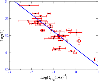
Table-1 below is the same as Table-4 of BS2007. Schaefer has compiled all the properties needed to calibrate the GRB events, which then produces the GRBs HD for any particular cosmology. Column (1) gives the six-digit GRB identification number in the usual format of YYMMDD. Column (2) gives the redshift ($z$) of the GRB rounded to the nearest 0.01. Column (3) is $P_{\textrm{bolo}}$  and its uncertainty in units of   c m   s .  Column (4) gives $S_{\textrm{bolo}}$  and its uncertainty in units of   c m .  Column (5) gives the beaming factor, $F_{\text{beam}}$. Column (6) gives the time lag for each burst in units of seconds in the Earth rest frame and its uncertainty. Column (7) gives the variability, $V$, and its uncertainty. Column (8) lists the observed $E_{\textrm{peak}}$  and its uncertainty, and finally Column (9) gives the minimun rise time,  $\tau_{\text{\tiny RT}}$ , in seconds in the Earth rest frame.

Table 1: Observables attained from Schaefer’s 69 GRBs sample

		$P_{\textrm{bolo}}$	$S_{\textrm{bolo}}$		$\tau_{\text{\tiny lag}}$		$E_{\textrm{peak}}$	$\tau_{\text{\tiny RT}}$
GRB	$z$	(  c m   s )	(  c m )	$F_{\text{beam}}$	( s )	$V$	( k eV )	( s )
(1)	(2)	(3)	(4)	(5)	(6)	(7)	(8)	(9)
970228$\ldots$$\ldots$	0.70	7.3E-6 $\pm$ 4.3E-7	$\cdots$	$\cdots$	$\cdots$	0.0059$\pm$0.0008	115${}_{-38}^{+38}$	0.26 $\pm$ 0.04
970508$\ldots$$\ldots$	0.84	3.3E-6 $\pm$ 3.3E-7	8.09E-6 $\pm$ 8.1E-7	0.0795$\pm$ 0.0204	0.50$\pm$0.30	0.0047$\pm$0.0009	389${}_{-[40]}^{+[40]}$	0.71 $\pm$ 0.06
970828$\ldots$$\ldots$	0.96	1.0E-5 $\pm$ 1.1E-6	1.23E-4 $\pm$ 1.2E-5	0.0053$\pm$ 0.0014	$\cdots$	0.0077$\pm$0.0007	298${}_{-[30]}^{+[30]}$	0.26 $\pm$ 0.07
971214$\ldots$$\ldots$	3.42	7.5E-7 $\pm$ 2.4E-8	$\cdots$	$\cdots$	0.03$\pm$0.03	0.0153$\pm$0.0006	190${}_{-[20]}^{+[20]}$	0.05 $\pm$ 0.02
980613$\ldots$$\ldots$	1.10	3.0E-7 $\pm$ 8.3E-8	$\cdots$	$\cdots$	$\cdots$	$\cdots$	92 ${}_{-42}^{+42}$	$\cdots$
980703$\ldots$$\ldots$	0.97	1.2E-6 $\pm$ 3.6E-8	2.83E-5 $\pm$ 2.9E-6	0.0184$\pm$ 0.0027	0.40$\pm$0.10	0.0064$\pm$0.0003	254${}_{-[25]}^{+[25]}$	3.60 $\pm$ 0.5
990123$\ldots$$\ldots$	1.61	1.3E-5 $\pm$ 5.0E-7	3.11E-4 $\pm$ 3.1E-5	0.0024$\pm$ 0.0007	0.16$\pm$0.03	0.0175$\pm$0.0001	604${}_{-[60]}^{+[60]}$	$\cdots$
990506$\ldots$$\ldots$	1.31	1.1E-5 $\pm$ 1.5E-7	$\cdots$	$\cdots$	0.04$\pm$0.02	0.0131$\pm$0.0001	283${}_{-[30]}^{+[30]}$	0.17 $\pm$ 0.03
990510$\ldots$$\ldots$	1.62	3.3E-6 $\pm$ 1.2E-7	2.85E-5 $\pm$ 2.9E-6	0.0021$\pm$ 0.0003	0.03$\pm$0.01	0.0100$\pm$0.0001	126${}_{-[10]}^{+[10]}$	0.14 $\pm$ 0.02
990705$\ldots$$\ldots$	0.84	6.6E-6 $\pm$ 2.6E-7	1.34E-4 $\pm$ 1.5E-5	0.0035$\pm$ 0.0010	$\cdots$	0.0210$\pm$0.0008	189${}_{-15}^{+15}$	0.05 $\pm$ 0.02
990712$\ldots$$\ldots$	0.43	3.5E-6 $\pm$ 2.9E-7	1.19E-5 $\pm$ 6.2E-7	0.0136$\pm$ 0.0034	$\cdots$	$\cdots$	65 ${}_{-10}^{+10}$	$\cdots$
991208$\ldots$$\ldots$	0.71	2.1E-5 $\pm$ 2.1E-6	$\cdots$	$\cdots$	$\cdots$	0.0037$\pm$0.0001	190${}_{-[20]}^{+[20]}$	0.32 $\pm$ 0.04
991216$\ldots$$\ldots$	1.02	4.1E-5 $\pm$ 3.8E-7	2.48E-4 $\pm$ 2.5E-5	0.0030$\pm$ 0.0009	0.03$\pm$0.01	0.0130$\pm$0.0001	318${}_{-[30]}^{+[30]}$	0.08 $\pm$ 0.02
000131$\ldots$$\ldots$	4.50	7.3E-7 $\pm$ 8.3E-8	$\cdots$	$\cdots$	$\cdots$	0.0053$\pm$0.0006	163${}_{-13}^{+13}$	0.12 $\pm$ 0.06
000210$\ldots$$\ldots$	0.85	2.0E-5 $\pm$ 2.1E-6	$\cdots$	$\cdots$	$\cdots$	0.0041$\pm$0.0004	408${}_{-14}^{+14}$	0.38 $\pm$ 0.06
000911$\ldots$$\ldots$	1.06	1.9E-5 $\pm$ 1.9E-6	$\cdots$	$\cdots$	$\cdots$	0.0235$\pm$0.0014	986${}_{-[100]}^{+[100]}$	0.05 $\pm$ 0.02
000926$\ldots$$\ldots$	2.07	2.9E-6 $\pm$ 2.9E-7	$\cdots$	$\cdots$	$\cdots$	0.0134$\pm$0.0013	100${}_{-7}^{+7}$	0.05 $\pm$ 0.03
010222$\ldots$$\ldots$	1.48	2.3E-5 $\pm$ 7.2E-7	2.45E-4 $\pm$ 9.1E-6	0.0014$\pm$ 0.0001	$\cdots$	0.0117$\pm$0.0003	309${}_{-12}^{+12}$	0.12 $\pm$ 0.03
010921$\ldots$$\ldots$	0.45	1.8E-6 $\pm$ 1.6E-7	$\cdots$	$\cdots$	0.90$\pm$0.30	0.0014$\pm$0.0015	89 ${}_{-13.8}^{+21.8}$	3.90 $\pm$ 0.50
011211$\ldots$$\ldots$	2.14	9.2E-8 $\pm$ 9.3E-9	9.20E-6 $\pm$ 9.5E-7	0.0044$\pm$ 0.0011	$\cdots$	$\cdots$	59 ${}_{-8}^{+8}$	$\cdots$
020124$\ldots$$\ldots$	3.20	6.1E-7 $\pm$ 1.0E-7	1.14E-5 $\pm$ 1.1E-6	0.0039$\pm$ 0.0010	0.08$\pm$0.05	0.0131$\pm$0.0026	87 ${}_{-12}^{+18}$	0.25 $\pm$ 0.05
020405$\ldots$$\ldots$	0.70	7.4E-6 $\pm$ 3.1E-7	1.10E-4 $\pm$ 2.1E-6	0.0060$\pm$ 0.0020	$\cdots$	0.0129$\pm$0.0008	364${}_{-90}^{+90}$	0.45 $\pm$ 0.08
020813$\ldots$$\ldots$	1.25	3.8E-6 $\pm$ 2.6E-7	1.59E-4 $\pm$ 2.9E-6	0.0012$\pm$ 0.0003	0.16$\pm$0.04	0.0131$\pm$0.0003	142${}_{-13}^{+14}$	0.82 $\pm$ 0.10
020903$\ldots$$\ldots$	0.25	3.4E-8 $\pm$ 8.8E-9	$\cdots$	$\cdots$	$\cdots$	$\cdots$	2.6${}_{-0.8}^{+1.4}$	$\cdots$
021004$\ldots$$\ldots$	2.32	2.3E-7 $\pm$ 5.5E-8	3.61E-6 $\pm$ 8.6E-7	0.0109$\pm$ 0.0027	0.60$\pm$0.40	0.0038$\pm$0.0049	80 ${}_{-23}^{+53}$	0.35 $\pm$ 0.15
021211$\ldots$$\ldots$	1.01	2.3E-6 $\pm$ 1.7E-7	$\cdots$	$\cdots$	0.32$\pm$0.04	$\cdots$	46 ${}_{-6}^{+8}$	0.33 $\pm$ 0.05
030115$\ldots$$\ldots$	2.50	3.2E-7 $\pm$ 5.1E-8	$\cdots$	$\cdots$	0.40$\pm$0.20	0.0061$\pm$0.0042	83 ${}_{-22}^{+53}$	1.47 $\pm$ 0.50
030226$\ldots$$\ldots$	1.98	2.6E-7 $\pm$ 4.7E-8	8.33E-6 $\pm$ 9.8E-7	0.0034$\pm$ 0.0008	0.30$\pm$0.30	0.0058$\pm$0.0047	97 ${}_{-17}^{+27}$	0.70 $\pm$ 0.20
030323$\ldots$$\ldots$	3.37	1.2E-7 $\pm$ 6.0E-8	$\cdots$	$\cdots$	$\cdots$	$\cdots$	44 ${}_{-26}^{+90}$	1.00 $\pm$ 0.50
030328$\ldots$$\ldots$	1.52	1.6E-6 $\pm$ 1.1E-7	6.14E-5 $\pm$ 2.4E-6	0.0020$\pm$ 0.0005	0.20$\pm$0.20	0.0053$\pm$0.0007	126${}_{-13}^{+14}$	$\cdots$
030329$\ldots$$\ldots$	0.17	2.0E-5 $\pm$ 1.0E-6	2.31E-4 $\pm$ 2.0E-6	0.0049$\pm$ 0.0009	0.14$\pm$0.04	0.0097$\pm$0.0002	68 ${}_{-2.2}^{+2.3}$	0.66 $\pm$ 0.08
030429$\ldots$$\ldots$	2.66	2.0E-7 $\pm$ 5.4E-8	1.13E-6 $\pm$ 1.9E-7	0.0060$\pm$ 0.0029	$\cdots$	0.0055$\pm$0.0057	35 ${}_{-8}^{+12}$	0.90 $\pm$ 0.20
030528$\ldots$$\ldots$	0.78	1.6E-7 $\pm$ 3.2E-8	$\cdots$	$\cdots$	12.5$\pm$0.50	0.0022$\pm$0.0019	32 ${}_{-5.0}^{+4.7}$	0.77 $\pm$ 0.20
040924$\ldots$$\ldots$	0.86	2.6E-6 $\pm$ 2.8E-7	$\cdots$	$\cdots$	0.30$\pm$0.04	$\cdots$	67 ${}_{-6}^{+6}$	0.17 $\pm$ 0.02
041006$\ldots$$\ldots$	0.71	2.5E-6 $\pm$ 1.4E-7	1.75E-5 $\pm$ 1.8E-6	0.0012$\pm$ 0.0003	$\cdots$	0.0077$\pm$0.0003	63 ${}_{-13}^{+13}$	0.65 $\pm$ 0.16
050126$\ldots$$\ldots$	1.29	1.1E-7 $\pm$ 1.3E-8	$\cdots$	$\cdots$	2.10$\pm$0.30	0.0039$\pm$0.0015	47 ${}_{-8}^{+23}$	3.90 $\pm$ 0.80
050318$\ldots$$\ldots$	1.44	5.2E-7 $\pm$ 6.3E-8	3.46E-6 $\pm$ 3.5E-7	0.0020$\pm$ 0.0006	$\cdots$	0.0071$\pm$0.0009	47 ${}_{-8}^{+15}$	0.38 $\pm$ 0.05
050319$\ldots$$\ldots$	3.24	2.3E-7 $\pm$ 3.6E-8	$\cdots$	$\cdots$	$\cdots$	0.0028$\pm$0.0022	$\cdots$	0.19 $\pm$ 0.04
050401$\ldots$$\ldots$	2.90	2.1E-6 $\pm$ 2.2E-7	$\cdots$	$\cdots$	0.10$\pm$0.06	0.0135$\pm$0.0012	118${}_{-18}^{+18}$	0.03 $\pm$ 0.01
050406$\ldots$$\ldots$	2.44	4.2E-8 $\pm$ 1.1E-8	$\cdots$	$\cdots$	0.64$\pm$0.40	$\cdots$	25 ${}_{-13}^{+35}$	0.50 $\pm$ 0.30
050408$\ldots$$\ldots$	1.24	1.1E-6 $\pm$ 2.1E-7	$\cdots$	$\cdots$	0.25$\pm$0.10	$\cdots$	$\cdots$	0.25 $\pm$ 0.08
050416$\ldots$$\ldots$	0.65	5.3E-7 $\pm$ 8.5E-8	$\cdots$	$\cdots$	$\cdots$	$\cdots$	15 ${}_{-2.7}^{+2.3}$	0.51 $\pm$ 0.30
050502$\ldots$$\ldots$	3.79	4.3E-7 $\pm$ 1.2E-7	$\cdots$	$\cdots$	0.20$\pm$0.20	0.0221$\pm$0.0029	93 ${}_{-35}^{+55}$	0.40 $\pm$ 0.20
050505$\ldots$$\ldots$	4.27	3.2E-7 $\pm$ 5.4E-8	6.20E-6 $\pm$ 8.5E-7	0.0014$\pm$ 0.0007	$\cdots$	0.0035$\pm$0.0019	70 ${}_{-24}^{+140}$	0.40 $\pm$ 0.15
050525$\ldots$$\ldots$	0.61	5.2E-6 $\pm$ 7.2E-8	2.59E-5 $\pm$ 1.3E-6	0.0025$\pm$ 0.0010	0.11$\pm$0.02	0.0135$\pm$0.0003	81 ${}_{-1.4}^{+1.4}$	0.32 $\pm$ 0.03
050603$\ldots$$\ldots$	2.82	9.7E-6 $\pm$ 6.0E-7	$\cdots$	$\cdots$	0.03$\pm$0.03	0.0163$\pm$0.0015	344${}_{-52}^{+52}$	0.17 $\pm$ 0.02
050802$\ldots$$\ldots$	1.71	5.0E-7 $\pm$ 7.3E-8	$\cdots$	$\cdots$	$\cdots$	0.0046$\pm$0.0053	$\cdots$	0.80 $\pm$ 0.20
050820$\ldots$$\ldots$	2.61	3.3E-7 $\pm$ 5.2E-8	$\cdots$	$\cdots$	0.70$\pm$0.30	$\cdots$	246${}_{-40}^{+76}$	2.00 $\pm$ 0.50
050824$\ldots$$\ldots$	0.83	9.3E-8 $\pm$ 3.8E-8	$\cdots$	$\cdots$	$\cdots$	$\cdots$	$\cdots$	11.0 $\pm$ 2.00
050904$\ldots$$\ldots$	6.29	2.5E-7 $\pm$ 3.5E-8	2.00E-5 $\pm$ 2.0E-6	0.0097$\pm$ 0.0024	$\cdots$	0.0023$\pm$0.0026	436${}_{-90}^{+200}$	0.60 $\pm$ 0.20
050908$\ldots$$\ldots$	3.35	9.8E-8 $\pm$ 1.5E-8	$\cdots$	$\cdots$	$\cdots$	$\cdots$	41 ${}_{-5}^{+9}$	1.50 $\pm$ 0.30
050922$\ldots$$\ldots$	2.20	2.0E-6 $\pm$ 7.3E-8	$\cdots$	$\cdots$	0.06$\pm$0.02	0.0033$\pm$0.0006	198${}_{-22}^{+38}$	0.13 $\pm$ 0.02
051022$\ldots$$\ldots$	0.80	1.1E-5 $\pm$ 8.7E-7	3.40E-4 $\pm$ 1.2E-5	0.0029$\pm$ 0.0001	$\cdots$	0.0122$\pm$0.0004	510${}_{-20}^{+22}$	0.19 $\pm$ 0.04
051109$\ldots$$\ldots$	2.35	7.8E-7 $\pm$ 9.7E-8	$\cdots$	$\cdots$	$\cdots$	$\cdots$	161${}_{-35}^{+130}$	1.30 $\pm$ 0.40
051111$\ldots$$\ldots$	1.55	3.9E-7 $\pm$ 5.8E-8	$\cdots$	$\cdots$	1.02$\pm$0.10	0.0024$\pm$0.0007	$\cdots$	3.20 $\pm$ 1.00
060108$\ldots$$\ldots$	2.03	1.1E-7 $\pm$ 1.1E-7	$\cdots$	$\cdots$	$\cdots$	0.0032$\pm$0.0058	65 ${}_{-10}^{+600}$	0.40 $\pm$ 0.20

Continued … $P_{bolo}$ $S_{bolo}$ $\tau_{\text{\tiny lag}}$ $E_{peak}$ $\tau_{\text{\tiny RT}}$ GRB $z$ (  c m   s ) (  c m ) $F_{beam}$ ( s ) $V$ ( k eV ) ( s ) (1) (2) (3) (4) (5) (6) (7) (8) (9) 060115$\ldots$$\ldots$ 3.53 1.3E-7 $\pm$ 1.6E-8 $\cdots$ $\cdots$ $\cdots$ $\cdots$ 62 ${}_{-6}^{+19}$ 0.40 $\pm$ 0.20 060116$\ldots$$\ldots$ 6.60 2.0E-7 $\pm$ 1.1E-7 $\cdots$ $\cdots$ $\cdots$ $\cdots$ 139${}_{-36}^{+400}$ 1.30 $\pm$ 0.50 060124$\ldots$$\ldots$ 2.30 1.1E-6 $\pm$ 1.2E-7 3.37E-5 $\pm$ 3.4E-6 0.0021$\pm$ 0.0002 0.08$\pm$0.04 0.0140$\pm$0.0020 237${}_{-51}^{+76}$ 0.30 $\pm$ 0.10 060206$\ldots$$\ldots$ 4.05 4.4E-7 $\pm$ 1.9E-8 $\cdots$ $\cdots$ 0.10$\pm$0.10 0.0025$\pm$0.0016 75 ${}_{-12}^{+12}$ 1.25 $\pm$ 0.25 060210$\ldots$$\ldots$ 3.91 5.5E-7 $\pm$ 2.2E-8 1.94E-5 $\pm$ 1.2E-6 0.0005$\pm$ 0.0001 0.13$\pm$0.08 0.0019$\pm$0.0004 149${}_{-35}^{+400}$ 0.50 $\pm$ 0.20 060223$\ldots$$\ldots$ 4.41 2.1E-7 $\pm$ 3.7E-8 $\cdots$ $\cdots$ 0.38$\pm$0.10 0.0075$\pm$0.0033 71 ${}_{-10}^{+100}$ 0.50 $\pm$ 0.10 060418$\ldots$$\ldots$ 1.49 1.5E-6 $\pm$ 5.9E-8 $\cdots$ $\cdots$ 0.26$\pm$0.06 0.0070$\pm$0.0005 230${}_{-[20]}^{+[20]}$ 0.32 $\pm$ 0.08 060502$\ldots$$\ldots$ 1.51 3.7E-7 $\pm$ 1.6E-7 $\cdots$ $\cdots$ 3.50$\pm$0.50 0.0010$\pm$0.0017 156${}_{-33}^{+400}$ 3.10 $\pm$ 0.30 060510$\ldots$$\ldots$ 4.90 1.0E-7 $\pm$ 1.7E-8 $\cdots$ $\cdots$ $\cdots$ 0.0028$\pm$0.0019 95 ${}_{-[30]}^{+[60]}$ $\cdots$ 060526$\ldots$$\ldots$ 3.21 2.4E-7 $\pm$ 3.3E-8 1.17E-6 $\pm$ 1.7E-7 0.0034$\pm$ 0.0014 0.13$\pm$0.03 0.0112$\pm$0.0039 25 ${}_{-[5]}^{+[5]}$ 0.20 $\pm$ 0.05 060604$\ldots$$\ldots$ 2.68 9.0E-8 $\pm$ 1.6E-8 $\cdots$ $\cdots$ 5.00$\pm$1.00 $\cdots$ 40 ${}_{-[5]}^{+[5]}$ 0.60 $\pm$ 0.20 060605$\ldots$$\ldots$ 3.80 1.2E-7 $\pm$ 5.5E-8 $\cdots$ $\cdots$ 5.00$\pm$3.00 $\cdots$ 169${}_{-[30]}^{+[200]}$ 2.00 $\pm$ 0.50 060607$\ldots$$\ldots$ 3.08 2.7E-7 $\pm$ 8.1E-8 $\cdots$ $\cdots$ 2.00$\pm$0.50 0.0059$\pm$0.0014 120${}_{-17}^{+190}$ 2.00 $\pm$ 0.20

III.1 Luminosity Relations and Calibration Procedure

The relationship between a measurable observable of the light curve (luminosity indicator) with the GRB luminosity is given by the relation luminosity in the form of a power-law, i. e., $L=B_{\text{lag}}\tau_{\text{\tiny lag}}^{a_{\text{lag}}}$,  $L=B_{\text{v}}V^{a_{\text{v}}}$, $L=B_{\text{peak}}E_{\textrm{peak}}^{a_{\text{peak}}}$, $E_{\gamma}=B_{\gamma,\text{peak}}E_{\textrm{peak}}^{a_{\gamma,\text{peak}}}$ and $L=B_{\text{\tiny RT}}\tau_{\text{\tiny RT}}^{a_{\text{\tiny RT}}}$. The observed (on Earth) luminosity indicators will have different values from those that would be abscribed in the rest frame of the GRB event. That is, the light curves and spectra seen by the Earth-orbiting satellites suffer time dilation and redshifting. Therefore, the physical connection between the indicators and the luminosity in the GRB rest frame must take into account the observed indicators and correct them to the rest frame of the GRB. For the temporal indicators, the observed quantities must be divided by $1+z$ to correct the time dilation. The observed $V$-value must be multiplied by $1+z$ because it varies inversely with time, and the observed $E_{\textrm{peak}}$ must be multiplied by $1+z$ to correct the redshift dilation of the spectrum. We have also used the same values employed by BS2007 for the luminosity indicators to minimize correlations between the normalization constant and the exponent during the fitting, i. e., for the temporal luminosity we use 0.1 s , for the variability 0.02, and for the energy indicator 300  k eV . Notice that these values are only valid for this data. Therefore, for another set of GRBs data we can not use them.

Figure 3: Variability-luminosity relation. The variability for 51 GRBs have been corrected to rest frame of each GRB event and plotted vs. the isotropic luminosity with the best-fit line (see Eq.23). This relation was verified by Schaeferschaefer2001 .

To explain the calibration procedure in general, we denote the five luminosity relations by $R_{i}=B_{i}\,Q_{i}^{a_{i}}$ and we take their logarithms to express them as a linear relation of the form

$$\log{R_{i}}=\log{B_{i}}+a_{i}\,\log{Q_{i}}\Rightarrow y_{i}=b+a\,x_{i}\;.$$

In order to use the linear regression method to determine the best-fit parameters we also take into account that in those luminosity relations these variables are independent. This feature allows to use the OLS Bisector method isobe1 . Besides, because the scatter of the data is consistent with a Gaussian distribution we can use the error propagation law: The optimum $\mathrm{bar}{f}$ for the quantity of interest $f(\alpha_{i})\,i=1,2,\ldots n$ calculated from the medians $\mathrm{bar}{\alpha_{i}}$ and their standard deviation $\sigma_{\mathrm{bar}{f}}$ is given by:error-propagation

$$\sigma_{\mathrm{bar}{f}}=\left[\sum_{i}^{n}\left(\frac{\partial f}{\partial\alpha_{i}}\right)^{2}\sigma^{2}_{\mathrm{bar}{\alpha}_{i}}\right]^{1/2}\;.$$ (15)

Then, for the luminosity indicators, applying this law, we obtain the standard deviation associated to the $x$-variable

$$\sigma_{x}=\left(\frac{d\,x(Q_{i})}{d\,Q_{i}}\right)\sigma_{\text{\tiny Q}_{i}}=\frac{1}{\ln{10}}\frac{\sigma_{\text{\tiny Q}_{i}}}{Q_{i}}\;.$$

Similarly, the standard deviation associated with the $y$-variable is function of $P_{\text{bolo}}$ when we use the burst luminosity Eq.(13), or is function of $S_{\textrm{bolo}}$  and $F_{\text{beam}}$ if we use the total collimation-corrected energy Eq.(14).

In the first case

$$\sigma_{y}=\frac{1}{\ln{10}}\frac{\sigma_{\text{\tiny P}_{\text{bolo}}}}{P_{\text{bolo}}}\;.$$ (16)

For the second case, corresponding to $\log{E_{\gamma}}$, the standard deviation is given by

$$\sigma_{y}=\frac{1}{\ln{10}}\sqrt{\left(\frac{\sigma_{\text{\tiny S}_{\text{bolo}}}}{\text{S}_{\text{bolo}}}\right)^{2}+\left(\frac{\sigma_{\text{\tiny F}_{\text{beam}}}}{F_{\text{beam}}}\right)^{2}}\;.$$ (17)

Then, the calibration will essentially be a linear fit on a log-log plot of the luminosity indicator $Q_{i}$ versus the burst luminosity $R_{i}$, i. e., we fit the line $y_{i}=b+a\,x_{i}$, and find the corrected value of the luminosity using the subroutine Sixlin.f isobe2   upon computing $\mathrm{bar}{y}_{i}(a,b,x_{i})$. Therefore, their associate error or standard deviation, using the Eq.(15), is given as

$$\sigma^{2}_{\mathrm{bar}{y}_{i}}=\sigma^{2}_{a}+(\sigma_{b}\,x_{i})^{2}+(b\sigma_{x_{i}})^{2}\;,$$ (18)

where $\sigma_{x_{i}}$ is given by Eq.(III.1).  As the uncertainties in both luminosities and their indicators are small than the observed scatter about the best-fit line, we must introduce an additional source of intrinsic scatter in the last expression, denoted by $\sigma_{\text{\tiny sys}}$. This value can be estimated by finding the value such that a $\chi^{2}$ fit of the luminosity calibration produces a reduced $\chi^{2}$ of unity

$$\chi^{2}=\frac{1}{N}\sum_{i}^{N}\frac{(\mathrm{bar}{y}_{i}-y_{i})^{2}}{\sigma^{2}_{\mathrm{bar}{y}_{i}}+\sigma^{2}_{\text{\tiny sys}}}\approx 1\;.$$ (19)

Here $\sigma^{2}_{\mathrm{bar}{y}_{i}}$ is given by Eq.(18) and then we re-cast the standard deviation for the correct luminosity as:

$$\sigma^{2}_{\mathrm{bar}{y}_{i}}=\sigma^{2}_{a}+(\sigma_{b}\,x_{i})^{2}+(b\sigma_{x_{i}})^{2}+\sigma^{2}_{\text{\tiny sys}}\;.$$ (20)

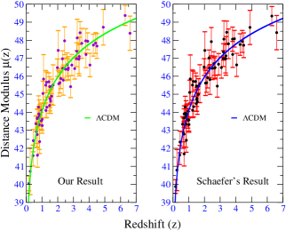
With the purpose of verifying our procedure we used the standard OLS method isobe1 in a barely different form to that one used by Schaefer (see pag.26 of BS2007), and then we calibrated the GRBs for the Concordance Cosmology (flat universe with $\Omega_{\textrm{m}}=0.27$ and $w=-1$). We choose $H_{0}=72$  k m   s M   from the HST Key projecthst . In Fig.1 we show our results and we compare them with the HD obtained by Schaefer (2007). One can notice that the difference between both plots is very small, what confirms that our method is self-consistent.

Figure 4: $E_{\textrm{peak}}$-luminosity relation. The $E_{\textrm{peak}}$values for 64 GRBs have been corrected to the rest frame of each GRB event and plotted versus the isotropic luminosity with the best-fit line, (see Eq.25). This relation was proposed and verified by Schaeferschaefer2003b ; bs2007 .

In the next subsections we present the results found with the calibration procedure of the five luminosity relations. All of them are based on an assumed Cardassian model using Eq.(II) with $\Omega_{\textrm{m}}=0.27,\,n=0.2$ and $H_{0}$ = 72  k m   s M 4.

III.1.1 Time lag versus Luminosity

The time lag, $\tau_{\text{lag}}$, was identified as a luminosity indicator by Norris et al. norris2000 who proposed a power law relation between the time lag and the isotropic luminosity. This relation is a consequence of the empirical/theoretical Liang-Kargatis relation liang1996 and was verified by Schaefer schaefer2001 . The calibration data are plotted in Fig.2 as $\log{\tau_{\text{lag}}/(1+z)}$ versus $L$. The best-fit linear regression line is also plotted. The equation for this calibration line reads:

$$\log{L}=52.23-1.00\log\left[{\frac{\tau_{\text{\tiny lag}}}{(1+z)0.1\mathrm{s}}}\right]\;.$$ (21)

Notice that the slope value satisfactorily agrees with the theoretical value of -1. The 1-$\sigma$ uncertainties in the intercept ($a=52.23$) and slopes ($b=-1.00$) are $\sigma_{a}=0.07$ and $\sigma_{b}=0.09$, and the uncertainty on the value of $\log{L}$ using Eq.(20) (the $\sigma^{2}_{\text{lag,sys}}$-value found is 0.36) is given by

$$\sigma^{2}_{\log{L}} = \sigma^{2}_{a}+\left\{\sigma_{b}\left[\frac{\tau_{\text{\tiny lag}}}{(1+z)0.1s}\right]\right\}^{2}\;,$$ (22)

$$+ \left(\frac{0.4343\,b\,\sigma_{\text{lag}}}{\tau_{\text{\tiny lag}}}\right)^{2}+\sigma^{2}_{\text{lag,sys}}\;.$$

III.1.2 Variability versus Luminosity

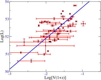
The variability ($V$) of a GRB event was identified as indicator luminosity by Fenimore & Ramirez-Ruiz fenimore2000 . Subsequently, Reitchart reichart2001 proposed a new relation between variability and isotropic luminosity, which is similar to the time lag-luminosity. Its origin is based in the physics of the relativistic shocked jetsmeszaros2002 ; kobayashi2002 . The calibration plot for the $V-L$ relation is given in Fig.3 along with the best-fit line. This best-fit can be represented by the equation

$$\log{L}=52.43+1.77\log\left[{\frac{V\,(1+z)}{0.02}}\right]\;.$$ (23)

The 1-$\sigma$ uncertainties in the intercept and slope are $\sigma_{a}=0.07$ and $\sigma_{b}=0.19$, the $\sigma_{V,\text{sys}}$ value found was 0.47 and the uncertainty in the log of the luminosity, using Eq.(20) is

$$\sigma^{2}_{\log{L}}=\sigma^{2}_{a}+\left\{\sigma_{b}\left[\frac{V\,(1+z)}{0.02}\right]\right\}^{2}+\left(\frac{0.4343\,b\,\sigma_{\text{v}}}{V}\right)^{2}+\sigma^{2}_{\text{v,sys}}\;.$$ (24)

Figure 5: $E_{\textrm{peak}}$-E_γ  relation, or Ghirlanda relation. The $E_{\textrm{peak}}$  values for 27 GRBs have been corrected to the rest frame of the GRB event and plotted versus the total burst energy in the $\gamma$-rays with the best-fit line (see Eq.27). This relation allows an empirical correction to the determined luminosity distance for each GRB event, in the same way as the light-curve shape correction for SNIa.

III.1.3 $E_{\textrm{peak}}$  versus Luminosity

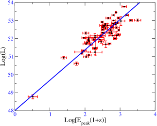
This luminosity relation was proposed by Schaeferschaefer2003b and is related to the instantaneus physics at the time of the peak. It was also verified in BS2007. The calibration plot for the $E_{\textrm{peak}}-L$ relation is given in Fig.4 along with the best-fit line. This best-fit line can be represented by the equation

$$\log{L}=52.18+1.68\log\left[{\frac{E_{\textrm{peak}}\,(1+z)}{300\,\mathrm{k}\mathrm{eV}}}\right]\;.$$ (25)

The 1-$\sigma$ uncertainties in the intercept and slope are $\sigma_{a}=0.05$ and $\sigma_{b}=0.10$, and the $\sigma_{E_{\textrm{peak}},\text{sys}}$ value is 0.4. The uncertainty in the log of the luminosity using Eq.(20) is

$$\sigma^{2}_{\log{L}} = \sigma^{2}_{a}+\left\{\sigma_{b}\left[\frac{E_{\textrm{peak}}\,(1+z)}{300\,\mathrm{k}\mathrm{eV}}\right]\right\}^{2}$$ (26)

$$+\left(\frac{0.4343\,b\,\sigma_{E_{\textrm{peak}}}}{E_{\textrm{peak}}}\right)^{2}+\sigma^{2}_{E_{\textrm{peak}},\text{sys}}\;.$$

III.1.4 $E_{\textrm{peak}}$ versus $E_{\gamma}$

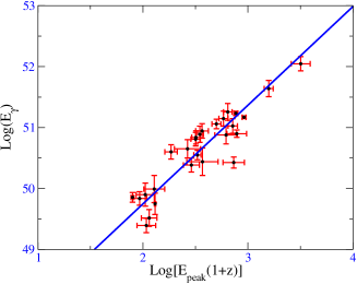
Ghirlanda et al. ghirlanda2004a found that for GRBs the total energy emitted in $\gamma$-rays (E_γ) after a proper collimated correction, correlates tightly with the peak energy $E_{\textrm{peak}}$  (in the $\nu$-F_ν spectrum). Thus the isotropically equivalent burst energy could be determined with sufficient accuracy to be used in a practically fashion for cosmological studies. The physics of this relation is explained within the standard jet modeleichler2004 ; yamazaki2004 ; rees2005 ; levinson2005 . The calibration plot for the $E_{\textrm{peak}}$-E_γ relation is given in Fig.5 along with the best-fit line. This best-fit can be represented with the equation

$$\log{E_{\gamma}}=50.52+1.68\log\left[{\frac{E_{peak}\,(1+z)}{300\,\mathrm{k}\mathrm{eV}}}\right]\;.$$ (27)

The 1-$\sigma$ uncertainties in the intercept and slope are $\sigma_{a}=0.05$ and $\sigma_{b}=0.10$, and $\sigma_{E_{\textrm{peak}},\text{sys}}=0.21$. The uncertainty in the log of the luminosity is obtained using the Eq.(20) is

$$\sigma^{2}_{\log{E_{\gamma}}} = \sigma^{2}_{a}+\left\{\sigma_{b}\left[\frac{E_{\textrm{peak}}\,(1+z)}{300\,\mathrm{k}\mathrm{eV}}\right]\right\}^{2}$$ (28)

$$+ \left(\frac{0.4343\,b\,\sigma_{E_{\textrm{peak}}}}{E_{\textrm{peak}}}\right)^{2}+\sigma^{2}_{E_{\textrm{peak}},\text{sys}}\;.$$

III.1.5 Rise Time versus Luminosity

In BS2007, in an effort to understand the physical origin of the variability, Schaefer calculated the variability for a wide range of simulate light curves constructed from individual pulses. He found that the most important determinant of the V-value was the rise time in the light curves, and this rise time can be connected with the physics of the shocked jet. The calibration plot for the $\tau_{\text{\tiny RT}}-L$ relation is given in Fig.6 along with the best-fit line. This best-fit can be represented with the equation

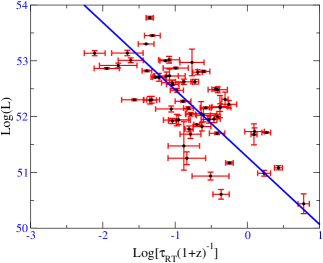
Figure 6: Minimum rise time-luminosity relation. The rise time for 62 GRBs have been corrected to the rest frame ofthe GRB event and plotted versus the isotropic luminosity with the best-fit line (see Eq.29). This relation was proposed and confirmed for Schaefer in BS2007.

$$\log{L}=52.48-1.21\log\left[{\frac{\tau_{\text{\tiny RT}}}{(1+z)\,0.1s}}\right]\;.$$ (29)

The 1-$\sigma$ uncertainties in the intercept and slope are $\sigma_{a}=0.07$ and $\sigma_{b}=0.11$, and the value of $\sigma_{RT,sys}=0.47$. The uncertainty in the log of the luminosity is given by Eq.(20)

$$\sigma^{2}_{\log{L}} = \sigma^{2}_{a}+\left\{\sigma_{b}\left[\frac{\tau_{\text{ \tiny RT}}}{(1+z)\,0.1s}\right]\right\}^{2}$$ (30)

$$+ \left(\frac{0.4343\,b\,\sigma_{\tau_{\text{\tiny RT}}}}{\tau_{\text{\tiny RT}}}\right)^{2}+\sigma^{2}_{\text{\tiny RT,sys}}\;.$$

In Table-2 we collect our results. Notice that they are very similar to the results obtained in BS2007 for the Concordance Cosmology ($\Omega_{\textrm{m}}=0.27$ and $w=-1$) and for the dark energy parametrization ($w_{0}=-1.31,w^{{}^{\prime}}=1.48$). Indeed, the set of $\chi^{2}$ for both methods are as follows: $\chi^{2}{\rm\Lambda-CDM/Schafer}=71.61248$, $\chi^{2}{\rm\Lambda-CDM/Schafer}_{\rm dof}=1.03786$, $\chi^{2}{\rm\Lambda-CDM/Ours}=72.16559$, $\chi^{2}{\rm\Lambda-CDM/Ours}_{\rm dof}=1.04587$, $\chi^{2}{\rm Card}=72.034$, $\chi^{2}{\rm Card}_{\rm dof}=1.04379$. This confirms one more time that the calibration procedure depends weekly of the input cosmology.

Table 2: Calibration Results

Luminosity Relation	$a$	$\sigma_{a}$	$b$	$\sigma_{b}$	$\sigma_{\text{\tiny sys}}$
$\tau_{\text{lag}}-L$	52.23	0.07	-1.00	0.09	0.36
$V-L$	52.43	0.07	1.77	0.19	0.47
$E_{\textrm{peak}}$-$L$	52.18	0.05	1.68	0.10	0.40
$E_{\textrm{peak}}$-Eγ	50.52	0.05	1.62	0.10	0.21
$\tau_{\text{\tiny RT}}-L$	52.48	0.07	-1.21	0.11	0.47

III.1.6 Combining the Derived Distance Moduli

After performing the calibration procedure for every $L$, or $E_{\gamma}$, we can also derive a luminosity distance, or equivalently their logarithms, and estimate their associate distance moduli using Eqs.(12,13,14) obtaining:

$$\mu(z) = \frac{5}{2}\log{(L)}-\frac{5}{2}\log{(4\pi\,P_{\text{bolo}})}+25\;,$$ (31)

$$\mu(z) = \frac{5}{2}\log{(E_{\gamma})}-\frac{5}{2}\log{\left(\frac{4\pi\,S_{\text{bolo}}\,F_{\text{beam}}}{1+z}\right)}\;.$$ (32)

The propagate uncertainties will depend on whether we calculate the distance modulus using $L$ or $E_{\gamma}$. Therefore, using Eq.(15), one can easily obtain

$$\sigma_{\mu}=2.5\,\left[\sigma^{2}_{\mathrm{bar}{y}}+\sigma^{2}_{y}\right]^{1/2}\;,$$ (33)

where $\sigma_{y}$ takes either the form of Eq.(16) if we calculate $L$, or the form of the Eq.(17) if we calculate $E_{\gamma}$, and $\sigma_{\mathrm{bar}{y}}$ is given by Eq.(20) applied to the respective luminosity relation.

With five luminosity indicators, each burst will have up to five estimated distance moduli an their 1-$\sigma$ uncertainties. As in BS2007, we label as $\mu_{1}\pm\sigma_{\mu_{1}}$,  $\mu_{2}\pm\sigma_{\mu_{2}}$,  $\mu_{3}\pm\sigma_{\mu_{3}}$,  $\mu_{4}\pm\sigma_{\mu_{4}}$,  $\mu_{5}\pm\sigma_{\mu_{5}}$, for the five indicators, respectively. Then to calculate the best estimate $\mu$ for each GRB event it is necessary to make a weight-average of all available distance moduli, which is given by:

$$\mu=\frac{1}{w}\sum_{i}^{5}w_{i}\mu_{i}\;,$$ (34)

where $w_{i}=1/\sigma^{2}_{i}\quad\textrm{and}\quad w=\sum_{i}^{5}w_{i}$

Then applying the error propagation law (see Eq.15) to Eq.(34) we obtain the standard deviation associate to this best estimate as $\sigma_{\mu}=1/\sqrt{w}$.

III.2 Hubble Diagram

In Table-3 we collect the distance moduli calculated for each burst. Columns (1) and (2) give the GRB event and their redshift ($z$), Column (3)-(7) give the distance modulus $\mu_{i}\pm\sigma_{\mu_{i}}$ calculated for each luminosity relation for the Cardassian cosmology: $\Omega_{\textrm{m}}=0.27$, $n=0.2$ and $H_{0}=72$ k m   s M   , and the Column (8) gives the combined distance modulus values obtained with the Eq.(34) and their uncertainties.

Table 3: Derived Distance Moduli

		$\mu_{1}$	$\mu_{2}$	$\mu_{3}$	$\mu_{4}$	$\mu_{5}$	$\mu$
GRB	$z$	(mag)	(mag)	(mag)	(mag)	(mag)	(mag)
(1)	(2)	(3)	(4)	(5)	(6)	(7)	(8)
970228$\ldots$$\ldots$	0.70	$\cdots$	42.41$\pm$1.23	42.31$\pm$1.19	$\cdots$	43.29$\pm$1.20	42.67$\pm$0.70
970508$\ldots$$\ldots$	0.84	43.00$\pm$1.14	42.99$\pm$1.26	45.54$\pm$1.05	43.78$\pm$0.66	42.94$\pm$1.21	43.77$\pm$0.43
970828$\ldots$$\ldots$	0.96	$\cdots$	42.85$\pm$1.21	43.96$\pm$1.05	43.47$\pm$0.66	43.14$\pm$1.24	43.43$\pm$0.47
971214$\ldots$$\ldots$	3.42	48.63$\pm$1.46	48.54$\pm$1.22	47.44$\pm$1.04	$\cdots$	49.17$\pm$1.32	48.31$\pm$0.62
980613$\ldots$$\ldots$	1.10	$\cdots$	$\cdots$	45.75$\pm$1.35	$\cdots$	$\cdots$	45.75$\pm$1.35
980703$\ldots$$\ldots$	0.97	44.42$\pm$0.97	44.81$\pm$1.20	45.98$\pm$1.04	43.45$\pm$0.61	42.00$\pm$1.25	44.02$\pm$0.41
990123$\ldots$$\ldots$	1.61	43.14$\pm$0.95	44.69$\pm$1.20	45.49$\pm$1.05	45.38$\pm$0.69	$\cdots$	44.78$\pm$0.46
990506$\ldots$$\ldots$	1.31	44.69$\pm$1.09	44.08$\pm$1.19	44.07$\pm$1.04	$\cdots$	43.80$\pm$1.21	44.18$\pm$0.56
990510$\ldots$$\ldots$	1.62	46.45$\pm$1.02	45.11$\pm$1.19	44.13$\pm$1.03	45.38$\pm$0.60	45.53$\pm$1.20	45.34$\pm$0.41
990705$\ldots$$\ldots$	0.84	$\cdots$	45.11$\pm$1.20	43.47$\pm$1.03	42.85$\pm$0.66	45.66$\pm$1.30	43.69$\pm$0.47
990712$\ldots$$\ldots$	0.43	$\cdots$	$\cdots$	41.75$\pm$1.07	41.41$\pm$0.69	$\cdots$	41.51$\pm$0.58
991208$\ldots$$\ldots$	0.71	$\cdots$	40.38$\pm$1.22	42.09$\pm$1.04	$\cdots$	41.88$\pm$1.20	41.52$\pm$0.66
991216$\ldots$$\ldots$	1.02	43.43$\pm$1.01	42.38$\pm$1.19	42.61$\pm$1.04	43.53$\pm$0.68	43.19$\pm$1.23	43.16$\pm$0.43
000131$\ldots$$\ldots$	4.50	$\cdots$	46.96$\pm$1.22	47.59$\pm$1.04	$\cdots$	48.34$\pm$1.37	47.58$\pm$0.69
000210$\ldots$$\ldots$	0.85	$\cdots$	40.78$\pm$1.22	43.68$\pm$1.03	$\cdots$	41.81$\pm$1.21	42.28$\pm$0.66
000911$\ldots$$\ldots$	1.06	$\cdots$	44.39$\pm$1.21	45.54$\pm$1.06	$\cdots$	44.66$\pm$1.31	44.94$\pm$0.68
000926$\ldots$$\ldots$	2.07	$\cdots$	46.12$\pm$1.22	44.13$\pm$1.03	$\cdots$	47.23$\pm$1.44	45.49$\pm$0.69
010222$\ldots$$\ldots$	1.48	$\cdots$	43.20$\pm$1.19	43.56$\pm$1.03	44.90$\pm$0.57	43.55$\pm$1.23	44.28$\pm$0.43
010921$\ldots$$\ldots$	0.45	42.76$\pm$1.02	40.86$\pm$2.42	43.07$\pm$1.07	$\cdots$	41.06$\pm$1.26	42.34$\pm$0.62
012111$\ldots$$\ldots$	2.14	$\cdots$	$\cdots$	46.96$\pm$1.06	44.98$\pm$0.67	$\cdots$	45.55$\pm$0.57
020124$\ldots$$\ldots$	3.20	47.73$\pm$1.18	48.37$\pm$1.28	46.14$\pm$1.07	46.39$\pm$0.67	47.22$\pm$1.23	46.88$\pm$0.44
020405$\ldots$$\ldots$	0.70	$\cdots$	43.90$\pm$1.19	44.40$\pm$1.12	43.41$\pm$0.79	42.56$\pm$1.21	43.55$\pm$0.52
020813$\ldots$$\ldots$	1.25	44.31$\pm$0.97	45.19$\pm$1.19	43.91$\pm$1.04	43.90$\pm$0.64	42.86$\pm$1.21	44.01$\pm$0.41
020903$\ldots$$\ldots$	0.25	$\cdots$	$\cdots$	40.65$\pm$1.29	$\cdots$	$\cdots$	40.65$\pm$1.29
021004$\ldots$$\ldots$	2.32	46.34$\pm$1.21	46.60$\pm$2.76	46.62$\pm$1.18	45.71$\pm$0.84	47.53$\pm$1.34	46.34$\pm$0.53
021211$\ldots$$\ldots$	1.01	43.98$\pm$0.94	$\cdots$	42.19$\pm$1.06	$\cdots$	44.45$\pm$1.21	43.51$\pm$0.61
030115$\ldots$$\ldots$	2.50	46.48$\pm$1.09	47.25$\pm$1.78	46.42$\pm$1.14	$\cdots$	45.36$\pm$1.29	46.29$\pm$0.63
030226$\ldots$$\ldots$	1.98	46.84$\pm$1.44	47.07$\pm$1.97	46.64$\pm$1.09	46.10$\pm$0.69	46.35$\pm$1.26	46.38$\pm$0.48
030323$\ldots$$\ldots$	3.37	$\cdots$	$\cdots$	46.74$\pm$1.58	$\cdots$	47.22$\pm$1.46	47.00$\pm$1.07
030328$\ldots$$\ldots$	1.52	45.13$\pm$1.43	44.61$\pm$1.22	44.84$\pm$1.04	44.49$\pm$0.64	$\cdots$	44.65$\pm$0.47
030329$\ldots$$\ldots$	0.17	41.94$\pm$0.98	41.55$\pm$1.20	39.57$\pm$1.03	38.81$\pm$0.61	40.49$\pm$1.21	39.97$\pm$0.41
030429$\ldots$$\ldots$	2.66	$\cdots$	47.65$\pm$2.33	45.44$\pm$1.14	46.44$\pm$0.89	46.57$\pm$1.26	46.28$\pm$0.59
030528$\ldots$$\ldots$	0.78	42.75$\pm$1.05	44.75$\pm$2.08	44.20$\pm$1.10	$\cdots$	46.08$\pm$1.26	44.19$\pm$0.62
040924$\ldots$$\ldots$	0.86	43.83$\pm$0.95	$\cdots$	42.60$\pm$1.04	$\cdots$	45.09$\pm$1.20	43.74$\pm$0.61
041006$\ldots$$\ldots$	0.71	$\cdots$	44.09$\pm$1.19	42.38$\pm$1.10	44.08$\pm$0.73	43.26$\pm$1.24	43.60$\pm$0.50
050126$\ldots$$\ldots$	1.29	45.37$\pm$0.98	46.74$\pm$1.41	45.77$\pm$1.08	$\cdots$	44.69$\pm$1.27	45.57$\pm$0.57
050318$\ldots$$\ldots$	1.44	$\cdots$	46.33$\pm$1.22	44.20$\pm$1.08	45.78$\pm$0.72	46.14$\pm$1.21	45.60$\pm$0.49
050319$\ldots$$\ldots$	3.24	$\cdots$	46.49$\pm$1.93	$\cdots$	$\cdots$	48.65$\pm$1.23	48.03$\pm$1.04
050401$\ldots$$\ldots$	2.90	46.06$\pm$1.15	46.94$\pm$1.22	45.22$\pm$1.06	$\cdots$	48.56$\pm$1.30	46.52$\pm$0.59
050406$\ldots$$\ldots$	2.44	48.16$\pm$1.19	$\cdots$	46.41$\pm$1.43	$\cdots$	48.96$\pm$1.45	47.87$\pm$0.77
050408$\ldots$$\ldots$	1.24	45.17$\pm$1.05	$\cdots$	$\cdots$	$\cdots$	45.76$\pm$1.27	45.40$\pm$0.81
050416$\ldots$$\ldots$	0.65	$\cdots$	$\cdots$	41.38$\pm$1.12	$\cdots$	45.22$\pm$1.43	42.83$\pm$0.88
050502$\ldots$$\ldots$	3.79	47.26$\pm$1.46	50.00$\pm$1.30	46.89$\pm$1.27	$\cdots$	47.16$\pm$1.39	47.87$\pm$0.67
050505$\ldots$$\ldots$	4.27	$\cdots$	46.97$\pm$1.59	46.86$\pm$1.21	48.43$\pm$0.99	47.60$\pm$1.30	47.63$\pm$0.61
050525$\ldots$$\ldots$	0.61	44.01$\pm$0.95	44.26$\pm$1.19	41.93$\pm$1.03	43.13$\pm$0.71	43.32$\pm$1.19	43.27$\pm$0.43
050603$\ldots$$\ldots$	2.82	45.69$\pm$1.45	45.60$\pm$1.23	45.48$\pm$1.07	$\cdots$	44.60$\pm$1.20	45.32$\pm$0.61
050802$\ldots$$\ldots$	1.71	$\cdots$	45.74$\pm$2.52	$\cdots$	$\cdots$	45.34$\pm$1.25	45.42$\pm$1.12
050820$\ldots$$\ldots$	2.61	45.87$\pm$1.05	$\cdots$	48.43$\pm$1.08	$\cdots$	44.97$\pm$1.26	46.55$\pm$0.65
050824$\ldots$$\ldots$	0.83	$\cdots$	$\cdots$	$\cdots$	$\cdots$	43.22$\pm$1.37	43.22$\pm$1.37
050904$\ldots$$\ldots$	6.29	$\cdots$	47.06$\pm$2.48	51.06$\pm$1.13	49.19$\pm$0.77	47.77$\pm$1.27	49.27$\pm$0.55
050908$\ldots$$\ldots$	3.35	$\cdots$	$\cdots$	46.82$\pm$1.06	$\cdots$	46.91$\pm$1.23	46.86$\pm$0.80
050922$\ldots$$\ldots$	2.20	46.46$\pm$1.01	43.91$\pm$1.25	45.86$\pm$1.04	$\cdots$	46.43$\pm$1.21	45.77$\pm$0.56
051022$\ldots$$\ldots$	0.80	$\cdots$	43.47$\pm$1.19	44.69$\pm$1.03	43.73$\pm$0.57	43.33$\pm$1.22	43.81$\pm$0.43
051109$\ldots$$\ldots$	2.35	$\cdots$	$\cdots$	46.59$\pm$1.11	$\cdots$	44.50$\pm$1.27	45.69$\pm$0.83
050922$\ldots$$\ldots$	1.55	44.90$\pm$0.96	44.64$\pm$1.35	$\cdots$	$\cdots$	43.71$\pm$1.30	44.52$\pm$0.67
060108$\ldots$$\ldots$	2.03	$\cdots$	46.90$\pm$3.83	46.87$\pm$1.52	$\cdots$	48.04$\pm$1.74	47.34$\pm$1.09
060115$\ldots$$\ldots$	3.53	$\cdots$	$\cdots$	47.34$\pm$1.04	$\cdots$	48.38$\pm$1.36	47.73$\pm$0.83
060116$\ldots$$\ldots$	6.60	$\cdots$	$\cdots$	49.29$\pm$1.28	$\cdots$	47.05$\pm$1.42	48.29$\pm$0.95
060124$\ldots$$\ldots$	2.30	46.83$\pm$1.09	47.39$\pm$1.24	46.89$\pm$1.10	46.96$\pm$0.69	46.03$\pm$1.27	46.87$\pm$0.45
060206$\ldots$$\ldots$	4.05	48.04$\pm$1.44	45.90$\pm$1.71	46.56$\pm$1.06	$\cdots$	45.71$\pm$1.22	46.53$\pm$0.65
060210$\ldots$$\ldots$	3.91	47.48$\pm$1.15	45.08$\pm$1.27	47.52$\pm$1.11	49.43$\pm$0.73	46.63$\pm$1.30	47.84$\pm$0.46
060223$\ldots$$\ldots$	4.41	47.47$\pm$0.99	48.94$\pm$1.48	47.39$\pm$1.07	$\cdots$	47.80$\pm$1.23	47.74$\pm$0.58
060418$\ldots$$\ldots$	1.49	44.90$\pm$0.96	45.19$\pm$1.20	45.99$\pm$1.04	$\cdots$	45.24$\pm$1.23	45.33$\pm$0.54
060502$\ldots$$\ldots$	1.51	43.60$\pm$1.08	42.99$\pm$3.53	46.81$\pm$1.19	$\cdots$	43.79$\pm$1.31	44.65$\pm$0.67
060510$\ldots$$\ldots$	4.90	$\cdots$	48.02$\pm$1.77	48.89$\pm$1.19	$\cdots$	$\cdots$	48.62$\pm$0.99
060526$\ldots$$\ldots$	3.21	48.22$\pm$0.98	49.09$\pm$1.38	44.88$\pm$1.10	46.83$\pm$0.82	48.53$\pm$1.24	47.29$\pm$0.47
060604$\ldots$$\ldots$	2.68	45.16$\pm$1.01	$\cdots$	46.56$\pm$1.07	$\cdots$	47.98$\pm$1.28	46.36$\pm$0.64
060605$\ldots$$\ldots$	3.80	45.14$\pm$1.26	$\cdots$	49.37$\pm$1.19	$\cdots$	46.44$\pm$1.34	47.11$\pm$0.73
060607$\ldots$$\ldots$	3.08	45.08$\pm$1.03	47.67$\pm$1.31	47.56$\pm$1.10	$\cdots$	45.35$\pm$1.25	46.33$\pm$0.58

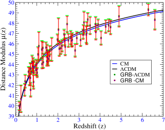
Fig.7 shows the HD for the GRBs calibrated with the Cardassian Cosmology. Notice that the observational data points are consistent with the Cardassian model predictions because its $\chi$-square per degree-of-freedom $\chi^{2}_{dof}\approx 1.00-1.07$ (see next section).

Figure 7: Hubble Diagram of 69 GRBs after having been calibrated with Cardassian Cosmology. The blue line corresponds to the HD predicted by the Cardassian parameters used in this calibration; $\Omega_{\textrm{m}}=0.27$,  $n=0.2$. The black line corresponds to the HD for the Concordance Cosmology ($\Lambda$-CDM model with $\Omega_{\textrm{m}}=0.27$,  $w=-1$). Here we assumed $H_{0}=72$  k m   s M .

Table 4: Best-fit analysis

Case	$\Omega_{\textrm{m}}$$\pm$$\sigma_{\Omega_{m}}$	n $\pm$$\sigma_{n}$	$\chi^{2}$	$\chi^{2}_{\text{dof}}$
exact $H_{0}$	0.45 $\pm$0.20 [${}^{+0.14}_{-0.09}$]	-0.70 $\pm$2.68 [${}^{+0.00}_{-0.00}$]	70.88	1.06
exact $H_{0}$,prior $\Omega_{\textrm{m}}$	0.28 $\pm$0.04 [${}^{+0.04}_{-0.04}$]	0.27 $\pm$0.16 [${}^{+0.14}_{-0.19}$]	71.53	1.07
Prior $H_{0}$	0.40 $\pm$0.36 [${}^{+0.25}_{-0.00}$]	0.26 $\pm$1.66 [${}^{+0.00}_{-0.00}$]	73.28	1.09
Prior $H_{0}$+${\cal R}$	0.35 $\pm$0.09 [${}^{+0.11}_{-0.08}$]	0.39 $\pm$0.22 [${}^{+0.22}_{-0.23}$]	73.29	1.09
Prior $H_{0}$.+${\cal A}$	0.33 $\pm$0.04 [${}^{+0.04}_{-0.04}$]	0.45 $\pm$0.29 [${}^{+0.26}_{-0.33}$]	73.30	1.09
Prior $H_{0}$.+${\cal R}$+${\cal A}$	0.32 $\pm$0.04 [${}^{+0.04}_{-0.04}$]	0.34 $\pm$0.16 [${}^{+0.14}_{-0.18}$]	73.50	1.10

IV Data Analysis: The Method

We can now determine the best-fit to the set of cosmological parameters $\theta=(\Omega_{\textrm{m}},n)$ after imposing several constraints. Later on we combine GRBs data with those from the CMB and BAO to put tigh constraints on these parameters. To this end, we construct the log-likelihood function $\chi^{2}$ by assuming hypothetical $m$ and $M$ magnitudes fitted to a number of redshifts:

$$\chi^{2}_{0}(\theta,H_{0},b_{i})=\sum_{i=1}^{N}\frac{[\mu_{te}(z_{i},\theta,H_{0})-\mu_{\text{dat}}(z)(z_{i},b_{1},\ldots,b_{5})]^{2}}{\sigma^{2}_{\mu_{\text{dat}}}(z_{i})}\;.$$ (35)

where $N$ is the number of data, $\mu_{\text{dat}}(z)$ and $\sigma_{\mu_{\text{dat}}}(z)$ are, respectively, the fitted distance modulus and its dispersion at redshift $z$ obtained from the calibration procedure. In addition, $\mu_{\text{th}}(z)$ is the theoretical prediction of the distance modulus and $b_{i}(i=1,\ldots,5)$ are the slopes obtained from the regression analysis.

We can obtain the function $\chi^{2}$ in the parameter space ($\theta,H_{0}$) by marginalizing over the five nuisance parameters $b_{i}$. However, a reasonable approximation is to consider the values of the slopes fixed at the values obtained in the regression analysis, because the GRB HD is nearly independent of the assumed cosmology. Therefore, the $\chi^{2}$ function reads

$$\chi^{2}_{0}(\theta,H_{0})=\sum_{i=1}^{N}\frac{(\mu_{\text{th}}(z_{i},\theta,H_{0})-\mu_{\text{fit}}(z_{i}))^{2}}{\sigma^{2}_{\mu_{\text{fit}}}(z_{i})}\;,$$ (36)

where $\mu_{\text{fit}}$ and $\sigma_{\mu_{\text{fit}}}$ are obtained in the previous section (see Eq.(34) and Column (8) in Table-3).

On the other hand, if we want to treat $\Omega_{\textrm{m}}$ as a free parameter with Gaussian prior distribution centered in $\Omega_{\textrm{m}}^{\text{true}}$ with spread $\sigma_{\Omega_{\textrm{m}}-\text{prior}}$ goliath , then we have to use

$$\chi^{2}_{\text{prior}}(\theta,H_{0})=\chi^{2}_{0}(\theta,H_{0})+\frac{(\Omega_{\textrm{m}}-\Omega_{\textrm{m}}^{\text{true}})^{2}}{\sigma^{2}_{\phantom{2}\Omega_{\textrm{m}}-\text{prior}}}\;.$$ (37)

IV.1 GRBs bounds $+$ constraints from other cosmological observations

To combine the GRBs data with the CMB we consider the model-independent shift-parameter ${\cal R}$, defined in terms of the $H_{0}$-independent luminosity distance: $D_{L}=H_{0}\,d_{L}$ (where $d_{L}$ is the proper luminosity distance)rcmb

$${\cal R}=\sqrt{\Omega_{\textrm{m}}}\frac{D_{L}(z_{r})}{1+z_{r}}=\sqrt{\Omega_{\textrm{m}}}\int_{0}^{z_{r}}\frac{dz}{E(z)}\;.$$ (38)

The shift-parameter ${\cal{R}}$ is related to the position of the first acoustic peak of the CMB anisotropy power spectrum but it can not be directly measured. However, its value is estimated from the data assuming a flat cosmology with dark matter and cosmological constant. The shift-parameter is defined, approximately, as the ratio of the sound horizon at recombination to the co-moving distance to the last scattering. The quantity $E(z)$ is given by Eq.(II) and $z_{r}$ = 1089 is the redshift of recombination. (From the three-year results of WMAP spergel Wang and Mukherjee estimated ${\cal R}$= 1.70 with spread $\sigma_{\cal R}=0.03$ wmuh ). Then, the statistical significance of a model is determined evaluating $\chi^{2}_{\cal R}=({\cal R}-1.70)^{2}/\sigma^{2}_{\cal R}$ together with the $\chi^{2}$ of the GRBs data, i. e.,

$$\chi^{2}=\chi^{2}_{0}(\theta,H_{0})+\chi^{2}_{\cal R}(\theta)\;.$$ (39)

Meanwhile, to combine the GRBs data with the BAO we considered the ${\cal A}$-parameter which describes the BAO peak in the matter perturbation power spectrum, given by eisen :

$${\cal A}=\sqrt{\Omega_{\textrm{m}}}\left[\frac{1}{z_{1}\,E^{1/2}(z_{1})}\int_{0}^{z_{1}}\frac{dz^{\prime}}{E(z^{\prime})}\right]^{2/3}\;,$$ (40)

where $z_{1}$ = 0.35 is the redshift at which the acoustic scale has been found. Eisenstein eisen found that the estimate value of the ${\cal A}$-parameter is ${\cal A}$= 0.469 with spread $\sigma_{\cal A}=0.017$. Similarly to the shift-parameter, the statistical significance of a model is then determined evaluating $\chi^{2}_{\cal A}=({\cal A}-0.469)^{2}/\sigma^{2}_{\cal A}$ together with the $\chi^{2}$ of the GRBs data, i. e.,

$$\chi^{2}=\chi^{2}_{0}(\theta,H_{0})+\chi^{2}_{\cal A}(\theta)\;.$$ (41)

This BAO peaks are clearly seen in the matter power spectrum, which together with the overall shape put tight constraints on the model parameters.

Therefore, if we combined the GRBs data plus CMB and BAO data the most general expression to $\chi^{2}$ is given by:

$$\chi^{2}(\theta,H_{0})=\chi^{2}_{0}(\theta,H_{0})+\chi^{2}_{\cal R}(\theta)+\chi^{2}_{\cal A}(\theta)\;.$$ (42)

To get the $\Omega_{\textrm{m}}-n$ parameter space we use the marginalization procedure choosing $H_{0}$ with Gaussian Prior distribution as nuissance parameter. Therefore, we can define a modified $\chi^{2}$-statistic by:

$$\tilde{\chi}^{2}(\theta)=-2\ln\left[\int_{0}^{\infty}dH_{0}\;\exp{[-0.5\chi^{2}(\theta,H_{0})]}\pi(H_{0})\right]\;,$$ (43)

where $\quad\pi(H_{0})=\frac{1}{\sqrt{2\pi\sigma^{2}_{H_{0}}}}\exp{\left(\frac{(H_{0}-72)^{2}}{2\,\sigma^{2}_{\phantom{2}H_{0}}}\right)}$. Here the function $\chi^{2}(\theta,H_{0})$ takes the form of Eqs.(36), (39), (41) or (42) depending on the analysis that will be performed. It is straightforward to minimize $\tilde{\chi}^{2}(\theta)$ using the base code MINUITjames or the function FindMinimum of the Software Mathematicamathematica to find $\chi^{2}_{min}(\theta)$, where $\chi^{2}_{min}$ is the minimum obtained for the best-fit parameters values $\mathrm{bar}{\theta}=(\mathrm{bar}{\Omega_{\textrm{m}}},\mathrm{bar}{n})$.

The variable $\chi^{2}_{min}$ is random in the sense that it depends on the random dataset that is used. Its probability distribution is a $\chi^{2}$ distribution for $N-\nu$ degrees of freedom ($\nu$ is the number of free parameters). This implies that the 68% of the random parameters in a given dataset will give a $\chi^{2}$ such that

$$\chi^{2}-\chi^{2}_{min}\leq\Delta\,\chi^{2}_{1\sigma}(\nu)\;,$$ (44)

where $\Delta\,\chi^{2}_{1\sigma}(\nu)$ is $2.3$ for two ($\nu=2$) free parameters. Thus, Eq.(44) defines the 1-$\sigma$ surface around the best-fit parameter. Similarly, it can be shown that 95.4% of the random numbers in the dataset will give a $\chi^{2}$ such that

$$\chi^{2}-\chi^{2}_{min}\leq\Delta\,\chi^{2}_{2\sigma}(\nu)\;,$$ (45)

where $\Delta\,\chi^{2}_{2\sigma}(\nu)$ is 6.17 for two free parameters. Thus, Eq.(45) defines the 2-$\sigma$ surface around the best-fit and similarly for higher $\sigma$’s.

The fixed values of $\Delta\,\chi^{2}_{i\sigma}$ ($i=1,2,\ldots$) determine the boundary of the $i$-th confidence-level contours and gives the probability of having a given $\chi^{2}$ for the true values of the estimate parameters laying inside the boundary. This criterion permit us to reject or accept any pair of ($\Omega_{\textrm{m}},n$) parameter, and if $\chi^{2}/(N-\nu)\approx 1$ the fit is said to be good and the data are said to be consistent with the considered cosmological model under consideration. We divide the statistical analysis in two subsections, considering the GRBs data alone and then combining GRBs with CMB and BAO data.

V Statistical analysis: Results

V.1 GRBs data alone

In this subsection we consider only the GRBs dataset for the following three cases, and perform their statistical analysis and construct their confidence-level contours, according to the method sketched above.

Figure 8: Confidence-level contours in the $\Omega_{m}-n$ parameter space for the flat Cardassian Model. The solid lines separate the 1-$\sigma$, 2-$\sigma$ and 3-$\sigma$ confidence-level (color) regions for the sole GRBs data, where the black point (0.45, -0.70) corresponds to the best fit. The encircling dashed lines divide the 1-$\sigma$, 2-$\sigma$ and 3-$\sigma$ confidence-level regions obtained after imposing the prior knowledge on $\Omega_{\textrm{m}}$, with the green point (0.28, 0.27) corresponding to the best-fit value, while the blue point (0.27, 0) corresponds to the cosmological constant $\Lambda$. One can see that in both cases the cosmological constant lies in the 2-$\sigma$ level.

exact $H_{0}$

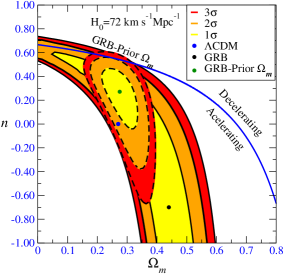
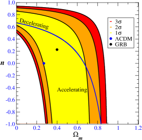
Here we suppose an exact knowledge of the Hubble parameter today. For the minimization procedure we use Eq.(36) obtaining $\chi^{2}_{\text{min}}$ = 70.88 ($\chi^{2}_{\text{dof}}$$=1.06$). In this case, we have two free parameters, the best-fit value corresponds to the point $(0.45,-0.7)$ in the $\Omega_{\textrm{m}}-n$ parameter space. The confidence contours are shown in the Fig.8. Hence, we see that the case $n=0$, which corresponds to the cosmological constant $\Lambda$, lies in the 2-$\sigma$ level.

exact $H_{0}$, prior $\Omega_{\textrm{m}}$

In this case we consider an exact knowledge of Hubble constant today and the matter density as free parameter with a uniform prior in the range $\Omega_{\textrm{m}}=0.27\pm 0.04$. The best-fit analysis was performed using Eq.(37) obtaining $\chi^{2}_{\text{min}}$ = 71.53 ($\chi^{2}_{\text{dof}}$$=1.07$), and the values correspond to the point ($0.28,0.27$) in the $\Omega_{\textrm{m}}-n$ parameter space. The confidence-level contours correspond to the filled regions limited by dashed lines in Fig.8. In this case, the point that corresponds to $\Lambda$ also lies in the 2-$\sigma$ level.

Prior $H_{0}$

Here the best-fit analysis is the most realistic constraint for GRBs. The minimization procedure was performed using the Eqs.(36) and (43) and the $\chi^{2}_{\text{min}}=73.28$, ($\chi^{2}_{\text{dof}}$$=1.09$). The best-fit value corresponds to the point ($0.40,0.26$) in the $\Omega_{\textrm{m}}-n$ parmeter space. The result in the $\Omega_{\textrm{m}}$-value agrees with the first one estimated by Schaefer in BS2007. The confidence-level contours correspond to the filled regions limited by solid lines in Figs.9,  10,  11 and 12. Hence, one can see that the cosmological constant lies in the 1-$\sigma$ level.

Figure 9: Idem to Fig.8, but now the black point (0.40, 0.26) corresponds the best-fit value, and the blue point (0.27, 0) corresponds to cosmological constant $\Lambda$. One can see that in this case the cosmological constant lies in the 1-$\sigma$ level.

V.2 Combined Data

In this subsection we analyze the role of the GRBs with combined constraints from the CMB and BAO data.

Prior $H_{0}$  and  ${\cal R}$

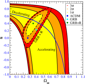
Here we perform the minimization procedure using Eq.(43) without $\chi^{2}_{\text{prior}}$ and $\chi^{2}_{\cal A}$, and found $\chi^{2}_{\text{min}}=73.29$, ($\chi^{2}_{\text{dof}}$$=1.09$). The best-fit value corresponds to the point ($0.35,0.39$), and the confidence contours are shown in the Fig.10. One can see that the relevant constraint on the parameter $n$, that would represent the dark energy and the cosmological constant $\Lambda$, lies in the 2-$\sigma$ level.

Figure 10: Confidence-level contours in the $\Omega_{\textrm{m}}-n$ parameter space for the flat Cardassian Model with GRBs $+$ ${\cal R}$. The solid lines separate the 1-$\sigma$, 2-$\sigma$ and 3-$\sigma$ confidence-level (color) regions for the GRBs data alone, with best-fit value ($0.40,0.26$) represented by the cyan point. The encircling dashed lines divide the 1-$\sigma$, 2-$\sigma$ and 3-$\sigma$ color-filled confidence regions of the bounds from GRBs + ${\cal R}$, with the best-fit value ($0.35,0.39$) represented by the green point. One can see that cosmological constant $\Lambda$ (blue point) lies in the 2-$\sigma$ level.

Prior $H_{0}$  and ${\cal A}$

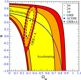
Here we perform the minimization procedure using Eq.(43) without $\chi^{2}_{\text{prior}}$ and $\chi^{2}_{\cal R}$, and found $\chi^{2}_{\text{min}}=73.30$, ($\chi^{2}_{\text{dof}}$$=1.09$). The best-fit value corresponds to the point ($0.33,0.45$) in the $\Omega_{\textrm{m}}-n$ parameter space, and the confidence contours are shown in Fig.11. We can see that the cosmological constant $\Lambda$ lies in the 1-$\sigma$ level.

Figure 11: Confidence-level contours in the $\Omega_{\textrm{m}}-n$ parameter space for the flat Cardassian Model with GRB plus ${\cal A}$. The solid lines separate the 1-$\sigma$, 2-$\sigma$ and 3-$\sigma$ confidence-level (color) regions for the GRBs data alone, with best-fit value ($0.40,0.26$) represented by the cyan point. The encircling dashed lines divide the 1-$\sigma$, 2-$\sigma$ and 3-$\sigma$ color-filled confidence regions of the bounds from GRBs plus ${\cal A}$, with the best-fit value ($0.33,0.45$) represented by the green point. One can see that cosmological constant $\Lambda$ (blue point) lies in the 1-$\sigma$ level.

Prior $H_{0}$,  ${\cal R}$  and ${\cal A}$

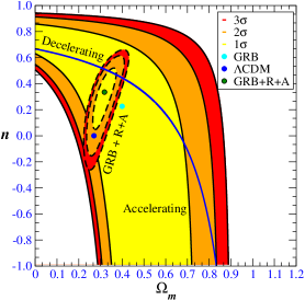
Here we consider the most general case for constraining the cosmological parameters with the combined data. In this case, we perform the minimization procedure using Eq.(43) without $\chi^{2}_{\text{prior}}$, the $\chi^{2}_{\text{min}}$ value is $73.50$ and ($\chi^{2}_{\text{dof}}$$=1.10$). The best-fit value corresponds to the point ($0.32,0.34$) in the $\Omega_{\textrm{m}}-n$ parameter space, and the confidence contours are shown in Fig.12. We can see that the cosmological constant $\Lambda$ lies in the 2-$\sigma$ level.

Figure 12: Confidence-level contours in the $\Omega_{\textrm{m}}$-n parameter space for the flat Cardassian Model with GRBs $+$ ${\cal R}$  $+$ ${\cal A}$. The solid lines separate the 1-$\sigma$, 2-$\sigma$ and 3-$\sigma$ confidence-level (color) regions for the GRBs data alone, with best-fit value ($0.40,0.26$) represented by the cyan point. The encircling dashed lines divide the 1-$\sigma$, 2-$\sigma$ and 3-$\sigma$ color-filled confidence regions of the bounds from the GRBs $\;+$ ${\cal R}$$\;+$ ${\cal A}$, with the best-fit value ($0.32,0.34$) represented by the green point. Hence, one can see that cosmological constant $\Lambda$ (blue point) lies in the 2-$\sigma$ level.

We collect our results for the several cases analyzed above in Table-4. One can see that our results are consistent with the result obtained by Bento et al. bento2005 , Gong and Duan gduan , Zhu et al. zhu . However in our analysis the cosmological constant lies in between 1-$\sigma$ and 2-$\sigma$.

VI Other observational aspects

Finally, we shall analyze the influence of the best-fit parameters on various cosmological parameters, including the Cardassian redshift of transition, which is one of the main observational features of that model.

Cardassian’s redshift

With the knowlegde of these best-fit parameters we calculate $z_{\text{card}}$  given by Eq.(8). Notice that this redshift is the one where the universe enters the phase of accelerate expansion driven by matter alone. This is the so-called Cardassian era. In general, it does not correspond to transition era to the accelerate expansion. Our results for the first three cases give $0.04<z_{\text{card}}<0.56$, in the most realistic case, where we considered the minimization procedure with the modified-$\chi^{2}$ for the GRBs data alone. For the combined data we obtain $0.41<z_{\text{card}}<0.55$. These results agree with the first initial values to $z_{\text{card}}$ given in the Table-I of the first Cardassian model proposed by Fresse and Lewis free , which was obtained by using observations of SNIa and the CMB. For each case, the values obtained for this redshift are given in Column (2) in the Table-5.

Deceleration Parameter

This parameter was introduced to characterize the dynamical evolution of the universe based on the sign of the second time derivative of the scale factor. It is defined as

$$q=-\frac{\ddot{a}a}{\dot{a}^{2}}\;.$$ (46)

The negative sign was put by-hand to come along with ancient ideas and “observations” suggesting that the universe was slowing down its expansion since the Big Bang. As we are interested in expressing it as a function of both the Hubble parameter and cosmological redshift we can easily rewrite Eq.(46) in the form:

$$q(z)=\frac{1}{2}\frac{(1+z)}{E^{2}(z)}\frac{d\,E^{2}(z)}{dz}-1\;.$$ (47)

It is clear that a negative value of this parameter stands for an accelerating universe, and conversely, a positive value implies a decelerating universe. For the Cardassian model we obtain

$$q(z)=\frac{1}{2}-\frac{3}{2}\frac{(1-n)\kappa(z)}{(1+\kappa(z))}\;,$$ (48)

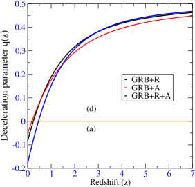
where $\kappa(z)=\left(\frac{\Omega_{\textrm{x}}}{\Omega_{\textrm{m}}}\right)(1+z)^{-3(1-n)}$. In Fig.13 we show the deceleration parameter as a function of the redshift for the values of the parameters obtained with the best-fit analysis.

The value $q_{0}\equiv q(z=0)$ indicates the expansion rythm today. In this case we obtain

$$q_{0}=\frac{1}{2}-\frac{3}{2}(1-n)\Omega_{\textrm{x}}\;.$$ (49)

The values obtained for this parameter lay in the range $-0.91<q_{0}<-0.05$ and are shown in Column (3) of Table-5.

The transition redshift $z_{\text{acc}}$ can be obtained by solving the equation $q(z)=0$. Our result agrees with the SNIa observations $0.18<z_{\text{acc}}<0.68$. The corresponding values are shown in Column (4) of Table-5.

Age of universe

Finally, we discuss the age-redshift relation in an alternatively form which is independent of the Hubble parameter today. To this purpose we use the measurement of the quantity $H_{0}\,t_{0}$:

$$H_{0}t_{0}=\int_{0}^{\infty}\frac{dz}{(1+z)E(z)}\;,$$ (50)

where the dimensionless function $E(z)$ is obtained from Eq.(II). Our result shows that $0.86<H_{0}\,t_{0}<0.94$ (see Column (5) in Table-5). In order to verify our result we have compared with several other estimates of the same parameter. For instance, the CMB alone contrains $t_{0}=13,7\pm 0.25$ spergel , while the Globular Cluster Age imposes $t_{0}=12.6^{3.4}_{-2.4}$ age2 for the age of universe. If we also assume that $H_{0}=h(9.77813\edad)^{-1}$, with $h=0.72\pm 0.08$ from the HST Key Project, and supposing that the $H_{0}$ and $t_{0}$ measurements are uncorrelated, we obtain for the product $H_{0}\,t_{0}$ the following range: $0.79<H_{0}\,t_{0}<1.27$ and $0.67<H_{0}\,t_{0}<1.31$, respectively. Clearly, one can see that our result is consistent with those estimates for the age of the universe.

Table 5: Other observational properties

Case	$z_{\text{card}}$	$q_{0}$	$z_{\text{acc}}$	$H_{0}t_{0}$
(1)	(2)	(3)	(4)	(5)
exact $H_{0}$	0.04	-0.91	0.37	0.90
exact $H_{0}$, prior $\Omega_{\textrm{m}}$	0.56	-0.29	0.68	0.94
Prior $H_{0}$	0.19	-0.20	0.34	0.88
Prior $H_{0}$+ ${\cal R}$	0.41	-0.08	0.24	0.90
Prior $H_{0}$+ ${\cal A}$	0.55	-0.05	0.18	0.86
Prior $H_{0}$+ ${\cal R}$+ ${\cal A}$	0.46	-0.18	0.46	0.89

VII Discussion and Conclusions

In the Cardassian model, the equivalent of the dark energy density arises from a modification of Friedmann’s equations through the introduction of a new function of the matter energy density in the form of an additional nonlinear term of mass. The outcoming model of the universe is then flat, matter dominated and accelerating.

Meanwhile, in order to understand the expansion history of the universe one needs to be able to trace it back in time up to very high redshifts and construct its Hubble diagram from light-emitting cosmic sources laying along the pathway to the Big Bang. In this perspective, GRBs offer a mean to extend up to redshifts $z>6$ the HD already built on SNIa observations $z<2$. GRBs are now known to have several light-curves (in different energy bands) and various spectral properties from which the luminosity of each burst can be calculated, once it is calibrated for a specific cosmology. This last procedure has been proved to be self-consistent bs2007 , and it turns GRBs useful standard candles for cosmographic studies.

(a) Deceleration parameter for GRBs data alone

(b) Deceleration parameter for combined GRBs + CMB data

Figure 13: Deceleration parameters for Cardassian model as a function of the redshift for the values of best-fit solution. The horizontal line, labeled (d)/(a) ($q(z)=0$), divide the region with (a) acelerating or (d) decelerating expansion at a given redshift. Clearly, we can see a transition from decelerating-to-accelerating universe in the range $0.18<z<0.7$, which is approximately the redshift range inferred from SNIa observations.

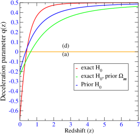
Following the same procedure used by Schaefer in BS2007, we made a simultaneous calibration with the Cardassian Cosmology of those GRB events that had their redshifts properly estimated. This allows us to construct the GRBs HD after using five empirical relations involving luminosity distance indicators of these GRBs. The results of the calibration procedure are shown in Figs.2-6. The Fig.1 states clearly that our method is self-consistent after comparing our results for the HD of GRBs calibrated with the concordance model with the one obtained by Schaefer bs2007 . The HD for the GRBs calibrated with the Cardassian model and its comparison with the $\Lambda$-CDM is presented in Fig.7. We can see that the data of observed GRB events are consistent with both models. The small difference can be considered negligible if one takes into account that ($a$) the $\chi^{2}$ for both calculations are quite similar, and ($b$) the error bar of each GRB event is still quite large.

We have also performed a detailed statistical analysis and constructed the confidence-level contours from these GRBs data after imposing several constraints on the cosmological parameters to be used for the analysis. First, considering exact knowledge of the Hubble parameter today, $H_{0}=72$ k m   s M   , the best-fit value obtained corresponds to the point $(0.45,-0.7)$ in the $\Omega_{\textrm{m}}-n$ parameter space. This point is shown in the associate confidence-level contour in Fig.8. The same figure shows the case where one considers also a uniform prior knowledge on the matter density ($\Omega_{\textrm{m}}=0.28\pm 0.04$), which corresponds to the point $(0.28,0.27)$. In Fig.9 we present the results of the analysis of the most specific case, that is, if one considers the lone GRBs dataset. We imposed a prior knowledge on the Hubble parameter today ($H_{0}=72\pm 8$ k m   s M ) , and the best-fit value obtained corresponds to the point ($0.40,0.26$). This result also agrees with the first one obtained by Schaefer (2007).

We have also analyzed the bounds from GRBs when combined with constraints provided by the CMB and BAO datasets. Considering the same prior knowledge on the Hubble parameter today, as we did before, the best-fit values obtained correspond to the points ($0.35,0.39$) in the case of GRBs + ${\cal R}$  (Fig.10), ($0.33,0.45$) in the case of GRBs $+$ ${\cal A}$  (Fig.11), and ($0.32,0.34$) in the case of GRBs $+$${\cal R}$$+$ ${\cal A}$  (Fig.12). The best-fit parameters obtained from this analysis are in agreement with those obtained from previous investigations that used SNIa data combined with CMB and BAO constraints.

Besides, with the knowledge of the best-fit parameters, we analyze their influence on other observational properties of this model. For the Cardassian redshift, our results for the first three cases (with fixed value of $H_{0}$) give $0.04<z_{\text{card}}<0.56$. For the combined data we obtained $0.41<z_{\text{card}}<0.55$. These results agree with the very first initial values of $z_{\text{card}}$ calculated by Freese and Lewis free , which was obtained by using observations of SNIa and the CMB. For the deceleration parameter, the values obtained lay in the range $-0.91<q_{0}<-0.05$. For the transition redshift $z_{\text{acc}}$ we obtained $0.18<z_{\text{acc}}<0.68$, which agrees with that inferred from SNIa observations. Finally, we obtained a couple of bounds for the age-redshift product $H_{0}\,t_{0}$: ($a$) $0.79<H_{0}\,t_{0}<1.27$ if one considers $t_{0}=13.7\pm 0.25$   from CMB spergel , and ($b$) $0.67<H_{0}\,t_{0}<1.31$, if one considers $t_{0}=12.6^{3.4}_{-2.4}$   from the Globular Cluster Age age2 . Our results are consistent with those estimates for the age of the universe.

In summary, the GRBs HD has been built to demonstrate the reliability of GRBs as an independent tool to check the consistency of most current cosmological models over distance scales not allowed to SNIa. This diagram for GRBs shows a great potential to make the GRBs observations a complementary tool to SNIa, large scale structure, baryon acoustic oscillations, an perhaps to CMB observations. In the near future, new studies based on these novel relations promise a major breakthrough in using GRBs to do precision cosmology.