Selfdecomposability and selfsimilarity:
a concise primer

Abstract

We summarize the relations among three classes of laws: infinitely divisible, selfdecomposable and stable. First we look at them as the solutions of the Central Limit Problem; then their role is scrutinized in relation to the Lévy and the additive processes with an emphasis on stationarity and selfsimilarity. Finally we analyze the Ornstein–Uhlenbeck processes driven by Lévy noises and their selfdecomposable stationary distributions, and we end with a few particular examples.

PACS numbers: 02.50.Cw, 02.50.Ey, 05.40.Fb

MSC numbers: 60E07, 60G10, 60G51, 60J75

Key Words: Selfsimilarity, Selfdecomposability, Lévy processes, Additive processes.

1 Notations and preliminary remarks

Selfsimilarity is a very popular research topics since a few years, and it has been approached from many different standpoints producing an unavoidable level of confusion [1]. The present paper is devoted to a short summary of the properties of some important and well known families of laws: infinitely divisible, selfdecomposable and stable (for details see for example [2, 3, 4, 5]). First of all we will recall their role in the formulation and in the solutions of the central limit problem: as we will see in the next section this amounts to a quest for all the limit laws of sums of independent random variables. Our families of distributions will then be analyzed by means of both their possible decompositions in other laws, and the explicit form of their characteristic functions: the celebrated Lévy–Khintchin formula. In particular it will be discussed the intermediate role played by the selfdecomposable laws between the more popular stable, and infinitely divisible distributions. We will then explore these laws in connection with the additive and the Lévy processes, looking for their importance with respect to both the properties of stationarity and selfsimilarity. In particular it will be recalled how from selfdecomposable distributions it is always possible to define both stationary and selfsimilar additive processes which – with the exception of important particular cases – will in general be different. A few remarks are also added to show the differences between this selfsimilarity and that of the well known fractional Brownian motion. We will also analyze the Ornstein–Uhlenbeck processes driven by these Lévy noises, and their stationary distributions which are always selfdecomposable. We will finally elaborate a few examples to illustrate these results, and to compare the behavior of our processes.

In what follows we will adopt the following notations (for details see for example [2, 6]): $X,Y,\ldots$ will denote the random variables, namely the measurable functions $X(\omega),Y(\omega),\ldots$ defined on a probability space $(\Omega,\mathcal{F},\mathbf{P})$ where $\Omega$ is a sample space, $\mathcal{F}$ is a $\sigma$–algebra of events and $\mathbf{P}$ a probability measure. We will then respectively write $F(x),G(y),\ldots$ for their cumulative distribution functions

$$F(x)=\mathbf{P}\{X\leq x\}\,,\quad G(y)=\mathbf{P}\{Y\leq y\}\,,\quad\ldots$$

and $\varphi(u),\chi(v),\ldots$ for their characteristic functions

$$\varphi(u)=\mathbf{E}\left(e^{iuX}\right)\,,\quad\chi(v)=\mathbf{E}\left(e^{ivY}\right)\,,\quad\ldots$$

where the symbol $\mathbf{E}$ denotes the expectation value of a random variable according to the probability $\mathbf{P}$, namely for example

$$\mathbf{E}(X)=\int_{\Omega}X(\omega)\,d\mathbf{P}=\int_{-\infty}^{+\infty}x\,F(dx)\,.$$

When they exist, $f(x),g(y),\ldots$ will be the probability density functions, and in that event we will have

$$F(x)=\int_{-\infty}^{x}f(z)\,dz\,,\qquad f(x)=F^{\prime}(x)\,,\qquad\mathbf{E}(X)=\int_{-\infty}^{+\infty}xf(x)\,dx\,.$$

A law will be indifferently specified either by its cumulative distribution function (or density function), or by its characteristic function. To say that a random variable $X$ is distributed according to a given law we will also write either $X\sim F(x)$ or $X\sim\varphi(u)$; if a family of laws is denoted by a specific symbol, say $\mathcal{L}$, then we also write $X\sim\mathcal{L}$ to say that $X$ is distributed according to one of these laws. When two random variables $X$ and $Y$ are identically distributed we will adopt the notation

$$X\stackrel{{\scriptstyle d}}{{=}}Y\,.$$

If a property is true with probability 1 we will also say that it is true $\mathbf{P}$–almost surely and we will adopt the notation $\mathbf{P}\hbox{-a.s.}$ A type of laws (see [2] Section 14) is a family of laws that only differ by a centering and a rescaling: in other words, if $\varphi(u)$ is the characteristic function of a law, all the laws of the same type have characteristic functions $e^{ibu}\varphi(au)$ with a centering parameter $b\in\mathbb{R}$, and a scaling parameter $a>0$ (we exclude here the sign inversions). In terms of random variables this means that the laws of $X$ and $aX+b$ (for $a>0$, and $b\in\mathbb{R}$) always are of the same type, and on the other hand that $X$ and $Y$ belong to the same type if it is possible to find $a>0$, and $b\in\mathbb{R}$ such that $Y\stackrel{{\scriptstyle d}}{{=}}aX+b$. We will also say that a random variable $X\sim\varphi(u)$ and its law are composed of $X_{1}\sim\varphi_{1}(u)$ and $X_{2}\sim\varphi_{2}(u)$ when $X_{1}$ and $X_{2}$ are independent and $X\stackrel{{\scriptstyle d}}{{=}}X_{1}+X_{2}$, or equivalently when $\varphi(u)=\varphi_{1}(u)\varphi_{2}(u)$; then $X_{1}$ and $X_{2}$ are also called components of $X$. Of course, in terms of distributions, a composition amounts to a convolution; then, for example, if $\mathcal{N}(a^{2},b)$ denotes a normal law with expectation $b$ and variance $a^{2}$, the composition of two normal laws will also be indicated as $\mathcal{N}(a_{1}^{2},b_{1})*\mathcal{N}(a_{2}^{2},b_{2})$. For the stochastic processes $X(t),Y(t),\ldots$ we will say that $X(t)$ and $Y(t)$ are identical in law when the systems of their finite–dimensional distributions are identical, and in this case we will write

$$X(t)\stackrel{{\scriptstyle d}}{{=}}Y(t)\,.$$

A process $X(t)$ is said to be stochastically continuous if for every $\epsilon>0$

$$\lim_{\Delta t\rightarrow 0}\mathbf{P}\left\{{|X(t+\Delta t)-X(t)|>\epsilon}\right\}=0,\qquad\forall\,t\geq 0.$$

where $\mathbf{P}\left\{{\ldots}\right\}$ denotes the probability for the increment $|X(t+\Delta t)-X(t)|$ of being larger that $\epsilon>0$. In this paper all our random variables and processes will be one dimensional.

In this exposition we do not pretend neither rigor, nor completeness: we just list the results and the properties that are important to compare, and we refer to the existing literature for proofs and details, and for a few hints about possible recent applications. In fact the aim of this paper is just to draw an outline showing – without embarrassing the reader with excessive technical details – the deep, but otherwise simple ideas which are behind the properties of our families of laws and the simplest procedures to build from them the most important classes of processes. We hope that this, with the aid of some telling examples, will be helpful to approach this field of research by clarifying the roles, the differences and the subtleties of these laws and processes.

2 The Central Limit Problem

2.1 The classical limit theorems

It is well known that there are three kinds of classical limit theorems (all along this paper wherever we speak of convergence it is understood that we speak of convergence in law) which are characterized by the form of the respective limit laws:

• the Law of Large Numbers with limit laws of the degenerate type $\delta_{b}$ with characteristic function

  $$\varphi(u)=e^{ibu};$$

• the Normal Central Limit Theorem whose limit laws are of the gaussian type $\mathcal{N}(a^{2},b)$ with

  $$\varphi(u)=e^{ibu}e^{-a^{2}u^{2}/2};$$

• and the Poisson Theorem whose limit laws are of the Poisson types $\mathcal{P}(\lambda;a,b)$ with

  $$\varphi(u)=e^{ibu}e^{\lambda(e^{iau}-1)}.$$ (1)

The exact statements of these theorems in their traditional formulations are reprinted in every handbook of probability (see for example [6] p. 323 and following), and we will not reproduce them once more. Remark however that in our list, while speaking of the type for the degenerate and the gaussian laws, we also referred to the types for the Poisson laws. In fact all the normal laws $\mathcal{N}(a^{2},b)$ with expectation $b\in\mathbb{R}$ and variance $a^{2}>0$ constitute a unique type, and the same is true for the family of all the degenerate laws. On the other hand the standard Poisson laws $\mathcal{P}(\lambda)=\mathcal{P}(\lambda;1,0)$ with different parameters $\lambda$ belong to different types: indeed we can not recover a law $\mathcal{P}(\lambda)$ from another $\mathcal{P}(\lambda^{\prime})$ (with $\lambda\neq\lambda^{\prime}$) just by means of a centering and a rescaling. In other words we could say that every Poisson law $\mathcal{P}(\lambda)$ with a given $\lambda$ generates – by centering and rescaling – a distinct type $\mathcal{P}(\lambda;a,b)$ with characteristic functions (1).

The particularities of the Poisson laws with respect to the other two families of limit laws are also apparent from their properties of composition and decomposition. For a family of laws (not necessarily a type) to be closed under composition means that the composition (convolution) of two laws of that family still belongs to the same family. On the other hand closure under decomposition means that if a law of the family is decomposed in two laws, these two components necessarily belong to the same family. The types of limit laws appearing in the classical limit theorems show an important form of closure under composition and decomposition summarized in the following result (see [2] p. 283): the degenerate and normal types are closed under compositions and under decompositions; the same is true for every family of Poisson laws $\mathcal{P}(\lambda;a,b)$ with the same $a$. The closure under composition is in fact an elementary property; not so for the closure under decomposition: the proofs for the normal and the Poisson case were given in 1935-37 by H. Cramér and D.A. Raikov respectively. The normal and Poisson composition and decomposition properties can then be stated by saying that

$$\mathcal{N}(a_{1}^{2},b_{1})*\mathcal{N}(a_{2}^{2},b_{2}) = \mathcal{N}(a_{1}^{2}+a_{2}^{2},b_{1}+b_{2})$$

$$\mathcal{P}(\lambda_{1};a,b_{1})*\mathcal{P}(\lambda_{2};a,b_{2}) = \mathcal{P}(\lambda_{1}+\lambda_{2};a,b_{1}+b_{2})$$

Hence it is also apparent that a type of Poisson laws never is closed under composition and decomposition: we are always obliged to switch from a Poisson type to another while composing and decomposing them.

It is important to remark, however, that the classical limit theorems are not the embodiment of these composition and decomposition properties only, but they are more far–reaching and profound statements. In fact not only these theorems deal with limits of sums of independent random variables of a type which in general is different from that of the eventual limit laws – the Poisson law is the limit of sums of Bernoulli 0–1 random variables, while the normal and degenerate laws are limits of sums of still more general random variables – but also the distribution of the sum of the $n$ random variables does not coincide with the limit law at every step $n$ of the limiting process, as happens instead in a simple decomposition.

2.2 Formulations of the Central Limit Problem

To formulate the Central Limit Problem (CLP) let us look at it first of all in terms of sequences of random variables: usually we take a sequence $X_{k}$ of random variables, and then the sequence of their sums $S_{n}=X_{1}+\ldots+X_{n}$. In this case when we go from $S_{n}$ to $S_{n+1}$ we just add another random variable $X_{n}$ without changing the previous sum $S_{n}$. However this is not the more general way to produce sequences of sums of random variables. Consider indeed a triangular array of random variables $X_{k}^{(n)}$

$$\begin{array}[]{l}X_{1}^{(1)}\\ X_{1}^{(2)}\,,\;\;X_{2}^{(2)}\\ \;\;\vdots\qquad\qquad\quad\ddots\\ X_{1}^{(n)}\,,\;\;X_{2}^{(n)}\;,\;\ldots\;,\;\;X_{n}^{(n)}\\ \;\;\vdots\qquad\qquad\qquad\qquad\qquad\ddots\\ \end{array}$$

with $n=1,2,\ldots$ and $k=1,2,\ldots,n$, and suppose that

1. in every row $n\in\mathbb{N}$ the random variables $X_{1}^{(n)},\ldots,X_{n}^{(n)}$ are independent,

2. the $X_{k}^{(n)}$ are uniformly, asymptotically negligible, namely that

   $$\max_{k}\,\mathbf{P}\left\{{|X_{k}^{(n)}|\geq\epsilon}\right\}\stackrel{{\scriptstyle n}}{{\longrightarrow}}0\,,\qquad\forall\,\epsilon>0.$$

Define now the consecutive sums

$$S_{n}=\sum_{k=1}^{n}X_{k}^{(n)}\,.$$ (2)

Then the central limit problem for consecutive sums of independent random variables (CLP₁) reads: find the family of all the limit laws of the consecutive sums (2) and the corresponding convergence conditions (see [2] p. 301-2). Three remarks are in order here:

• for a given $n\in\mathbb{N}$ the random variables $X_{1}^{(n)},\ldots,X_{n}^{(n)}$ are independent, but in general they are neither identically distributed, nor of the same type;

• going from the row $n$ to the row $n+1$ the random variables and their laws change: in general $X_{k}^{(n)}$ and $X_{k}^{(n+1)}$ are neither identically distributed, nor of the same type; as a consequence going from $S_{n}$ to $S_{n+1}$ we not only add the $n+1$-th random variable, but we also are obliged to adjourn the law of $S_{n}$;

• the uniformly, asymptotically negligible condition is an important technical requirement added to avoid trivial answers to the CLP₁ (see for example [2] p. 302); in fact without this condition it is easy to show that any law $\varphi$ would be limit law of the consecutive sums (2): it would be enough for every $n$ to take $X_{1}^{(n)}\sim\varphi$, and $X_{k}^{(n)}=0\,\;\mathbf{P}\hbox{-a.s.}$ for $k>1$. The uniformly, asymptotically negligible condition will tacitly be assumed all along this paper.

Important particular cases of the CLP₁ are then selected when we specialize the sequence $X_{k}^{(n)}$ in the following way (see [2] p. 331): let us suppose that there is a sequence $X_{k}$, $k=1,2,\ldots$, of independent (but in general not identically distributed) random variables, and two sequences of numbers $a_{n}>0$ and $b_{n}\in\mathbb{R}$, $n=1,2,\ldots$, such that for every $k$ and $n$

$$X_{k}^{(n)}=\frac{1}{a_{n}}\left(X_{k}-\frac{b_{n}}{n}\right).$$ (3)

It is apparent that now going from $n$ to $n^{\prime}$ we just get a centering and a rescaling of every $X_{k}$, so that $X_{k}^{(n)}$ and $X_{k}^{(n^{\prime})}$ always are of the same type. Then the consecutive sums take the form of normed sums (namely centered and rescaled sums) of independent random variables

$$S_{n}=\sum_{k=1}^{n}X_{k}^{(n)}=\sum_{k=1}^{n}\frac{1}{a_{n}}\left(X_{k}-\frac{b_{n}}{n}\right)=\frac{1}{a_{n}}\left(\sum_{k=1}^{n}X_{k}-b_{n}\right)=\frac{\widetilde{S}_{n}-b_{n}}{a_{n}}$$ (4)

where we adopt the notation

$$\widetilde{S}_{n}=\sum_{k=1}^{n}X_{k}.$$

Then the central limit problem for normed sums of independent random variables (CLP₂) reads: find the family of all the limit laws of the normed sums (4) and the corresponding convergence conditions. Finally there is a still more specialized formulation of the central limit problem when we add the hypothesis that the random variables $X_{k}$ are not only independent, but also identically distributed (see [2] p. 338): in this case we speak of a central limit problem for normed sums of independent and identically distributed random variables (CLP₃).

2.3 Solutions of the Central Limit Problem

The answers to the different formulations of the central limit problem need the definition of several important families of laws that are much more general than the Gaussian type, and that can be defined by means of the properties of their characteristic functions. Suppose that $\varphi(u)$ is the characteristic function of a law: we will say that this law is infinitely divisible (see [2] p. 308) if for every $n\in\mathbb{N}$ we can always find another characteristic function $\varphi_{n}(u)$ such that

$$\varphi(u)=[\varphi_{n}(u)]^{n}.$$

Apparently the name comes from the fact that our law can always be decomposed in an arbitrary number of identical laws; remark however that for different values of $n$ we get in general laws $\varphi_{n}(u)$ of different types. In terms of random variables if $X\sim\varphi(u)$ is infinitely divisible, then for every $n\in\mathbb{N}$ we can find $n$ independent and identically distributed random variables $X_{1}^{(n)},\ldots,X_{n}^{(n)}$ all distributed as $\varphi_{n}(u)$ and such that

$$X\stackrel{{\scriptstyle d}}{{=}}\sum_{k=1}^{n}X_{k}^{(n)},$$

namely $X$ is always decomposable (in distribution) in the sum of an arbitrary, finite number of independent and identically distributed random variables. Let us call $\mathcal{F}_{ID}$ the family of all the infinitely divisible laws. Many important distributions are infinitely divisible: degenerate, Gaussian, Poisson, compound Poisson, geometric, Student, Gamma, exponential and Laplace are infinitely divisible. On the other hand the uniform, Beta and binomial laws are not infinitely divisible: in fact no distribution (other than the degenerate) with bounded support can be infinitely divisible (see [5] p. 31). Remark that if $\varphi(u)$ is an infinitely divisible characteristic function, then also $\varphi^{\lambda}(u)$ is an infinitely divisible characteristic function for every $\lambda>0$ (see [5] p. 35): we will see that this is instrumental to connect the infinitely divisible laws to the Lévy processes.

A second important family of laws selected by their decomposition properties is that of the selfdecomposable laws (see [2] p. 334): a law $\varphi(u)$ is selfdecomposable when for every $a\in(0,1)$ we can always find another characteristic function $\varphi_{a}(u)$ such that

$$\varphi(u)=\varphi(au)\varphi_{a}(u).$$ (5)

In terms of random variables this means that if $X\sim\varphi(u)$ is selfdecomposable, then for every $a\in(0,1)$ we can always find two independent random variables, $X^{\prime}\stackrel{{\scriptstyle d}}{{=}}X$ and $Y_{a}\sim\varphi_{a}(u)$, such that

$$X\stackrel{{\scriptstyle d}}{{=}}aX^{\prime}+Y_{a}\,.$$

In other words for every $a\in(0,1)$ $X$ can always be decomposed into two independent random variables such that one of them is of the same type of $X$. It can be shown that every selfdecomposable law, along with all its components, is also infinitely divisible (see [2] p. 335), so that if we call $\mathcal{F}_{SD}$ the family of all the selfdecomposable laws, then $\mathcal{F}_{SD}\subseteq\mathcal{F}_{ID}$. The Gaussian, Student, Gamma, exponential and Laplace laws are examples of selfdecomposable laws (see [5] p. 98). On the other hand the Poisson laws are not selfdecomposable: they only are infinitely divisible.

Finally we will say that a law $\varphi(u)$ is stable (see [2] p. 338) if for every $c_{1}>0$ and $c_{2}>0$ we can find $a>0$ and $b\in\mathbb{R}$ such that

$$e^{ibu}\varphi(au)=\varphi(c_{1}u)\varphi(c_{2}u).$$

This means now that if $X\sim\varphi(u)$ is stable, then for every $c_{1}>0$ and $c_{2}>0$ we can find two independent random variables $X_{1}\stackrel{{\scriptstyle d}}{{=}}X$ and $X_{2}\stackrel{{\scriptstyle d}}{{=}}X$, and two number $a>0$ and $b$ such that

$$aX+b\stackrel{{\scriptstyle d}}{{=}}c_{1}X_{1}+c_{2}X_{2}.$$

In other words we can always decompose a stable law in other laws which are of the same type as the initial one. Our definition can also be reformulated in a slightly different way (see [5] p. 69): for every $c>0$ we can always find $a>0$ and $b\in\mathbb{R}$ such that

$$e^{ibu}\varphi(au)=[\varphi(u)]^{c},$$

and this apparently means that for every $c>0$ the law $[\varphi(u)]^{c}$ is of the same type as $\varphi(u)$. A law is also said strictly stable if for every $c>0$ always exists $a>0$ such that

$$\varphi(au)=[\varphi(u)]^{c}.$$ (6)

All the stable laws are selfdecomposable, and hence if $\mathcal{F}_{St}$ is the family of all the stable laws we will have $\mathcal{F}_{St}\subseteq\mathcal{F}_{SD}$. In fact our classification of laws in only three families (infinitely divisible, selfdecomposable and stable) is an oversimplification of a much richer structure explored for example in [5], Chapter 3. Among the classical laws only the Gaussian and the Cauchy laws are stable.

Remark that if a law $\varphi$ belongs to one of our families, then also all its type belongs to the same family. Hence it would be more suitable to say that $\mathcal{F}_{ID}$, $\mathcal{F}_{SD}$ and $\mathcal{F}_{St}$ are families of types of laws; however in the following, for the sake of simplicity, this will be understood without saying. The relevance of our three families of laws lies in the fact that they represent the answers to the three formulations of the central limit problem discussed in the previous section. In fact it can be shown that $\mathcal{F}_{ID}\,,\,\mathcal{F}_{SD}$ and $\mathcal{F}_{St}$ exactly coincide with the families of the limit laws sought for respectively in CLP₁, CLP₂ and CLP₃ (see for example [2] p. 321, p. 335 and p. 339 for the three statements). To summarize these results – a few examples will be shown in the Section 4.2 – we can then say that:

• the laws of the normed sums (4) of sequences $X_{k}$ of independent and identically distributed random variables converge toward stable laws; in particular: when the $X_{k}$ have finite variance their normed sums converge – according to the classical theorem – to normal laws, while the non Gaussian, stable distributions are limit laws only for sums of random variables with infinite variance; a well known example of the non Gaussian limit laws is the Cauchy distribution;

• the laws of the normed sums (4) of sequences $X_{k}$ of independent, but not necessarily identically distributed, random variables converge toward selfdecomposable laws; the special case of the stable laws is recovered when the $X_{k}$ are also identically distributed; in other words when a selfdecomposable law is not stable it can not be the limit law of normed sums of independent and identically distributed random variables;

• finally the laws of the consecutive sums (2) of triangular arrays $X_{k}^{(n)}$ converge to infinitely divisible laws: a classical example of non selfdecomposable convergence is represented by the Poisson Limit Theorem recalled in the Section 2.1; of course the selfdecomposable case is obtained when the triangular array has the form (3) and the consecutive sums become normed sums (4); however infinitely divisible laws which are not selfdecomposable (as the Poisson law) can not be limit laws of normed sums of independent random variables.

Nothing forbids, of course, that in this scheme a Gaussian law be also the limit law for consecutive sums of triangular arrays that do not reduces to normed sums. To complete the picture we will hence just recall here that there are also necessary and sufficient conditions for the convergence to normal laws of triangular arrays of independent, but not necessarily identically distributed, random variables with finite variances (see [6] p. 326).

Since the stable distributions are limit laws of normed sums (4) of independent and identically distributed random variables we can also introduce the notion of domain of attraction of a stable law $\varphi_{S}\,$: we will say that a law $\varphi$ belongs to the domain of attraction of $\varphi_{S}$ when we can find two sequences of numbers, $a_{n}>0$ and $b_{n}$, such that the normed sums (4) of a sequence $X_{k}$ of random variables all distributed as $\varphi$, converge to $\varphi_{S}$. Remark that this definition can not be immediately extended to the non stable distributions which are not limit laws of normed sums of independent and identically distributed random variables, so that we can not speak of a unique distribution $\varphi$ being attracted by the limit law.

Every law with finite variance belongs to the domain of attraction of the normal law (see [2] p. 363). It is also important to stress here that, while all stable laws are attracted by themselves (see [2] p. 363), a non stable, infinitely divisible law $\varphi$ – which always is in itself the limit law of a suitable consecutive sum (2) of some triangular array of random variables – also belongs to the domain of attraction of some stable law $\varphi_{S}$: normed sums (4) of random variables all distributed as $\varphi$ will converge toward some stable law $\varphi_{S}$. For instance the Poisson law – which is an infinitely divisible limit law, as the Poisson Theorem shows – apparently also is in the domain of attraction of the normal law since it has a finite variance: a normed sum of random variables all distributed according to the same Poisson law will converge to the Gauss law. Finally we recall, without going into more detail, that for a given law $\varphi$ it is always possible to find if it belongs to some domain of attraction, and then it is also possible to find both the stable limit law $\varphi_{S}$, and the admissible numerical sequences $a_{n}>0$ and $b_{n}$ entering in the normed sums (4) converging to $\varphi_{S}$ (see [2] p. 364).

2.4 The Lévy–Khintchin formula

It is not easy to find out if a given law $\varphi(u)$ belongs to one of the families defined in the previous section just by looking at the definitions introduced up to now. It is important then to recall the explicit form of the characteristic functions of our families of laws given by the Lévy–Khintchin formula. It can be proved (see [2] p. 343) indeed that the logarithmic characteristic $\psi(u)=\log\varphi(u)$ of an infinitely divisible law is uniquely associated, through the formula

$$\psi(u)=iu\gamma-\frac{\beta^{2}}{2}\,u^{2}+\lim_{\delta\rightarrow 0}\int_{|x|>\delta}\left(e^{iux}-1-\frac{iux}{1+x^{2}}\right)\,dL(x)$$ (7)

to a generating triplet $\left(\beta^{2},L,\gamma\right)$ where $\gamma,\,\beta\in\mathbb{R}$, and the Lévy function $L(x)$ is defined on $\mathbb{R}\backslash\{0\}$, is non decreasing on $(-\infty,0)$ and $(0,+\infty)$, with $L(\pm\infty)=0$ and

$$\lim_{\delta\rightarrow 0}\int_{\delta<|y|<x}y^{2}\,dL(y)<+\infty$$

for $x>0$ finite. In other words a law will be infinitely divisible if and only if its logarithmic characteristic satisfies the relation (7) for a suitable choice of $\left(\beta^{2},L,\gamma\right)$. The Lévy function $L(x)$ also defines the Lévy measure (for details see [5] Section 8)

$$\nu(B)=\int_{B}dL(x)$$

for every measurable set $B$ of $\mathbb{R}$ and $\nu\left(\{0\}\right)=0$, so that often we will refer to $\left(\beta^{2},\nu,\gamma\right)$ as the generating triplet. When the Lévy measure $\nu$ is absolutely continuous we will also denote by $W(x)=L^{\prime}(x)$ its density. Remark that the Lévy–Khintchin formula (7) can be given in a variety of equivalent versions (see [5] p. 37) by suitably choosing the integrand functions, but we will not go into such details.

For a given law even the verification of the formula (7) is not in general an easy task. In the case of stable laws, however, the Lévy–Khintchin formula is considerably simpler since it no longer explicitely involves integrals on the Lévy measure. A stable law is characterized by a parameter $0<\alpha\leq 2$ (see [5] p. 76) and it is then also said $\alpha$–stable ($\alpha$-stable): the case $\alpha=2$ corresponds to the Gaussian laws, and to a vanishing Lévy measure. In the non Gaussian $\alpha$–stable cases ($0<\alpha<2$) on the other hand the Lévy measure is not zero, it is absolutely continuous and we have (see [5] p. 80)

$$dL(x)=W(x)\,dx=\left\{\begin{array}[]{ll}A\,x^{-1-\alpha}dx,&\hbox{for $x>0$,}\\ B|x|^{-1-\alpha}dx,&\hbox{for $x<0$,}\end{array}\right.$$

with $A\geq 0,\;B\geq 0$ and $A+B>0$. Finally in both cases – Gaussian and non Gaussian – the logarithmic characteristic must satisfy the following relation (see [5] p. 86)

$$\psi(u)=\begin{cases}iau-b|u|^{\alpha}\left(1-i\,\mathrm{sign}\left({u}\right)c\tan\frac{\pi}{2}\alpha\right)&\text{if $\alpha\neq 1$},\\ iau-b|u|\left(1+i\,\mathrm{sign}\left({u}\right)\frac{2}{\pi}\,c\log|u|\right)&\text{if $\alpha=1$},\end{cases}$$

where $\alpha\in(0,2]$, $a\in\mathbb{R}$, $b>0$ and $|c|\leq 1$. The Gaussian case simply corresponds to $\alpha=2$. When the law is also symmetric the characteristic function is real and the formula reduces itself to the quite elementary expression

$$\varphi(u)=e^{-b|u|^{\alpha}}\,,\qquad 0<\alpha\leq 2\,.$$ (8)

The form of the Lévy–Khintchin formula, or equivalently of the triplet $\left(\beta^{2},L,\gamma\right)$, of the selfdecomposable laws, on the other hand, is not so simple. They in fact play in some sense a sort of intermediate role between the generality of the infinitely divisible laws and the special properties of the stable laws. It can be proved indeed (see [5] p. 95) that a law is selfdecomposable if and only if its Lévy measure is absolutely continuous and its density is

$$W(x)=L^{\prime}(x)=\frac{k(x)}{|x|}$$ (9)

where the function $k(x)$ is non negative, is increasing on $(-\infty,0)$ and is decreasing on $(0,+\infty)$. By the way this also show why a Poisson law (whose Lévy measure is not absolutely continuous) can not be selfdecomposable. As a consequence the Lévy–Khintchin formula  (7) of the selfdecomposable laws is more specialized than that of the general infinitely divisible laws, but it still contains a non elementary integral part.

3 Lévy processes and additive processes

An additive process $X(t)$ is a stochastically continuous process with independent increments and $X(0)=0\,,\;\mathbf{P}\hbox{-a.s.}$ (namely the probability of not being zero vanishes); on the other hand a Lévy process is an additive process with the further requirement that the increments must be stationary (for further details see [5] Section 1). The stationarity of the increments means that the law of $X(s+t)-X(s)$ does not depend on $s$. Processes with independent increments are also Markov processes, and hence the entire family of their joint laws at an arbitrary, finite number of times can be deduced just from the one– and the two–times distributions. In other words it is enough to know the laws of the increments to have the complete law of the process. This of course is a very good reason to be interested in Markov, and in particular in additive processes, but it must be recalled here that there are also non Markovian processes which can still be defined by means of very simple tools. An important example that will be briefly mentioned later is the fractional Brownian motion which takes advantage of being a Gaussian process to make up for its lack of Markovianity. It is also important to recall here that – with the exception of Gaussian processes – the additive processes trajectories can make jumps. This does not contradict their stochastic continuity because the jumping times are random, and hence, for every $t$, the probability of a jump occurring exactly at $t$ is zero.

3.1 Stationarity and infinitely divisible laws

In the following the law of the process increment $X(t)-X(s)$ will be given by means of its characteristic function $\phi_{s,t}(u)$, so that the stationarity of the Lévy processes simply entails that $\phi_{s,t}(u)$ only depends on the difference $\tau=t-s$: in this case we will use the shorthand, one–time notation $\phi_{\tau}(u)$. As for every Markov process the laws of the increments of an additive process must satisfy the Chapman–Kolmogorov equations which for the characteristic functions are

$$\phi_{r,t}(u)=\phi_{r,s}(u)\phi_{s,t}(u)\,,\qquad 0\leq r<s<t\,;$$ (10)

for Lévy (stationary) processes these equations take the form

$$\phi_{\sigma+\tau}(u)=\phi_{\sigma}(u)\phi_{\tau}(u)\,,\qquad\sigma,\tau>0\,.$$ (11)

There is now a very simple and intuitive procedure to build a Lévy process: take the characteristic function $\varphi(u)$ of a law and define

$$\phi_{t}(u)=\left[\varphi(u)\right]^{t/T}.$$ (12)

It is immediate to see that $\phi_{t}(u)$ satisfies (11), so that it can surely be taken as the characteristic function of the stationary increments of a Lévy process. Here $T$ plays the role of a dimensional time constant (a time scale) introduced to have a dimensionless exponent. To have a consistent procedure, however, we must be sure that when $\varphi(u)$ is a characteristic function, also $\phi_{t}(u)$ in (12) is a characteristic function for every $t>0$, but unfortunately this is simply not true for every characteristic function $\varphi(u)$. We are led hence to ask for what kind of characteristic functions (12) is again a characteristic function. We know, on the other hand, that if $\varphi$ is an infinitely divisible characteristic function, then also $\varphi^{\lambda}$ with $\lambda>0$ is a characteristic function, and an infinitely divisible one too. In fact it is possible to show that (12) is a characteristic function if and only if $\varphi(u)$ is infinitely divisible. In other words there is a one-to-one relation between the class $\mathcal{F}_{ID}$ of the infinitely divisible laws and that of the Lévy processes (see [5] Section 7). Remark however that in general for a Lévy process defined by (12) the infinitely divisible law of the increments at a generic time $t$ is neither $\varphi(u)$, nor of the same type of $\varphi(u)$. Only at $t=T$ the law is necessarily $\varphi(u)$, while for $t\neq T$ it can be rather different and – but for few well known cases – its explicit cumulative distribution function (or density function) could be quite difficult to find.

On the other hand when $\varphi(u)$ is a stable law it is easy to see from the very definition (6) of stability that at every time $t$ the law of the increments (12) will always belong to the same type (this is famously what happens for the Gauss and Cauchy laws). In this case we speak of a stable process, and its evolution can be summarized just in the time dependence of the law parameters which will produce a trajectory inside a unique type. A different situation arises instead when $\varphi(u)$ only belongs to a family of infinitely divisible laws closed under composition and decomposition. As we have already remarked these families do not in general constitute a type (as the family of the Poisson laws $\mathcal{P}(\lambda)$): if however they are closed under composition (as are both the Poisson and the Compound Poisson processes) the law (12) of the increment of the Lévy process stays in the same family of laws all along an evolution which is described by the time dependence of the law parameters; this however does not amount to the stability of the process since our family is not a single type.

Since every Lévy process is associated to an infinitely divisible law $\varphi(u)=e^{\psi(u)}$, and since every infinitely divisible law is associated to a generating triplet $\left(\beta^{2},\nu,\gamma\right)$ we will also speak of the logarithmic characteristic $\psi(u)$ and of the generating triplet $\left(\beta^{2},\nu,\gamma\right)$ of a Lévy process. In this case however the Lévy measure $\nu$ has also an important probabilistic meaning w.r.t. the Lévy process (see for example [7] pp. 75-85): for every Borel set $A$ of $\,\mathbb{R}$, $\nu(A)$ represents the expected number, per unit time, of (non-zero) jumps with size belonging to $A$. It can also be proved that for every compact set A such that $0\notin A$ we have $\nu(A)<+\infty$, namely the number of jumps per unit time of finite (neither infinite, nor infinitesimal) size is finite. Remark however that this does not mean that $\nu$ is a finite measure on $\mathbb{R}$: in fact the function $L(x)$ associated to $\nu$ can diverge in $x=0$ so that the process can have an infinite number of infinitesimal jumps in every compact $[0,T]$. In this case, when $\nu(\mathbb{R})=+\infty$, we speak of an infinite activity process, and the set of the jump times of every trajectory will be countably infinite and dense in $[0,+\infty]$. For the sake of simplicity we will not introduce here the important Lévy–Itô decomposition of a Lévy process into its continuous (Gaussian) and jumping (Poisson) parts: the readers are referred to [7], Section 3.4 for a synthetic treatment.

3.2 Selfsimilarity and selfdecomposable laws

A process $X(t)$ (possibly neither additive, nor stationary) is said to be selfsimilar when for every given $a>0$ we can find $b>0$ such that

$$X(at)\stackrel{{\scriptstyle d}}{{=}}bX(t),$$

namely when every change $a$ in the time scale can be compensated in distribution by a corresponding change $b$ in the space scale. In terms of the increment characteristic functions this means that for every $a>0$ we must have a $b>0$ such that

$$\phi_{as,at}(u)=\phi_{s,t}(bu).$$ (13)

In fact it can be proved more about the form of this space–time compensation: given a selfsimilar process we can always find $H>0$ such that $b=a^{H}$ (see [5] p. 73). This number $H$ is called the exponent of the process or Hurst index, and we will also speak of $H$–selfsimilar processes. For further details about selfsimilar, additive processes see also [8].

Since a Lévy process is completely specified by (12) as characteristic function of its increments, then in this case the selfsimilarity means that for every $a>0$ it exists $b>0$ such that

$$[\varphi(u)]^{at/T}=[\varphi(bu)]^{t/T}.$$ (14)

From the definition (6) of the strictly stable laws and from (14) it is easy to understand then that the unique selfsimilar Lévy processes must be strictly stable. For instance in a Wiener process we have $\varphi(u)=e^{-u^{2}\sigma^{2}/2}$, namely

$$[\varphi(u)]^{t/T}=e^{-u^{2}Dt/2},\qquad D=\frac{\sigma^{2}}{T}\,,$$

and hence

$$[\varphi(u)]^{at/T}=e^{-u^{2}Dat/2}$$

so that $b=\sqrt{a}$ (namely $H=1/2$) is the required compensation. This means that, insofar as the coefficient $D$ remains the same, we can change the space and time scales $\sigma$ and $T$ (namely we can change the units of measure) without changing the Wiener process distribution. More precisely than these simple remarks, it can be proved that a Lévy process $X(t)$ is selfsimilar if and only if it is strictly stable (see [5] p. 71).

Things are rather different, however, when we consider only additive (not necessarily Lévy) processes, namely when we can also live without stationarity. Now we must stick to the general selfsimilarity equation (13), and we must remark again that there is another simple, intuitive procedure producing additive (but not necessarily stationary), selfsimilar processes: simply consider a characteristic function $\varphi(u)$, a real number $H>0$ and take

$$\phi_{s,t}(u)=\frac{\varphi\left(\left(t/T\right)^{H}u\right)}{\varphi\left(\left(s/T\right)^{H}u\right)}\,.$$ (15)

It is now apparent that the characteristic functions of this family satisfy the equation (10) and are also selfsimilar according to the definition (13) with the space–time scale compensation produced by $b=a^{H}$. Namely (15) produces an $H$–selfsimilar process. Of course we must ask here the same question surfaced w.r.t. equation (12) in the case of stationary processes: when can we be sure that the function defined by the ratio (15) of two characteristic function still is the bona fide characteristic function of a law? Even in this case, however, the answer can be hinted to by looking at the definition (5) of a selfdecomposable characteristic function$\,.$ More precisely it can be proved that (15) is a characteristic function if and only if $\varphi(u)$ is selfdecomposable (see [5] p. 99): this ultimately brings out the intimate relation connecting selfsimilarity and selfdecomposability.

Since selfdecomposable laws are also infinitely divisible the previous remarks show that from a given selfdecomposable $\varphi(u)$ we can always produce two different kinds of processes: a Lévy process whose stationary increments follow the law (12); and a family of additive, selfsimilar process – one for every value of $H>0$ – whose (possibly non stationary) increments follow the law (15). All these processes generated from the same $\varphi(u)$ are in general different with one exception: when $\varphi(u)$ is an $\alpha$–stable law the associated Lévy process coincide with the $H$–selfsimilar one with Hurst index $H=1/\alpha$. In this last case indeed the characteristic functions (12) and (15) are identical (to see it take for example the symmetric form (8) of a stable characteristic function). Remark also that the index of an $\alpha$–stable law always satisfies $0<\alpha\leq 2$ ($\alpha=2$ for the Gaussian law), and that this is coherent with the limitation $H=1/\alpha\geq 1/2$ for the Hurst index of the stable, selfsimilar processes (see [5] p. 75). On the other hand, in every other case (either non–stable, or $\alpha$–stable with $\alpha\neq 1/H$), from a selfdecomposable law $\varphi(u)$ we can always build a Lévy, non selfsimilar process from (12), and a family of additive, selfsimilar processes with non stationary increments from (15). Finally from a infinitely divisible, but not selfdecomposable law we can only get a Lévy process from (12), but no selfsimilarity is allowed. For more details about present interest of the selfdecomposable distributions and selfsimilar processes in the applications see for instance [9] and [10].

Remark that selfsimilarity is not tied to the dependence or independence of the increments: we have seen here that among independent increment processes we find both selfsimilar and non selfsimilar processes; and on the other hand a process can be selfsimilar without showing independence of the increments. A celebrated example of this second case is the so called fractional Brownian motion: this is a centered, Gaussian, $H$–selfsimilar (for $H\in[0,1]$) process $B(t)$ with stationary increments, and covariance function

$$\mathbf{E}\left[{B(t)B(s)}\right]=\frac{|t|^{2H}+|s|^{2H}-|t-s|^{2H}}{2}\,,\qquad\quad t,s>0.$$

It is apparent that this is nothing else than a generalization of the well known covariance function of the usual Brownian motion $\mathbf{E}\left[{B(t)B(s)}\right]=\min(t,s)$ that is recovered when $H=1/2$. Since $B(t)$ is centered and Gaussian, this covariance function is all that is needed to define the process also if it is not Markovian. In fact a fractional Brownian motion coincides with the usual Brownian motion (and hence is Markovian with independent increments) only for $H=1/2$, while for $H\neq 1/2$ it is non–Markovian, has correlated increments and for $H>1/2$ shows long–range dependence. In other words an $H$–selfsimilar fractional Brownian motion with $H\neq 1/2$ is neither additive, nor Markovian: in fact it is not even a semimartingale, and hence few results of stochastic calculus can be used. From another standpoint (see [7] p. 230) we can say that the selfsimilarity can have different origins: it can stem either from the length of the distribution tails of independent increments, or from the correlation between short–tailed, Gaussian increments, and the two effects can also be mixed. For more information about the fractional Brownian motion see [11] and [12]

3.3 Selfdecomposable laws and Ornstein–Uhlenbeck processes

Selfdecomposable laws appear also in another important context: they are the most general class of stationary distributions of processes of the Ornstein–Uhlenbeck type. Take a Lévy process $Z(t)$ with generating triplet $(a^{2},\mu,c)$ and logarithmic characteristic $\chi(u)$, and for $b>0$ consider the stochastic differential equation (for simplicity we take $T=1$)

$$dX(t)=-bX(t)\,dt+dZ(t),\quad\qquad X(0)=X_{0}\quad\mathbf{P}\hbox{-a.s.}$$ (16)

whose exact meaning is rather in its integral form

$$X(t)=X_{0}-b\int_{0}^{t}X(s)\,ds+Z(t).$$

When $Z(t)$ is a Wiener process the equation (16) coincides with the stochastic differential equation of an ordinary, Gaussian Ornstein–Uhlenbeck process; but the equation (16) keeps the meaning of a well behaved stochastic differential equation even if $Z(t)$ is a generic, non Gaussian Lévy process, and its solution

$$X(t)=X_{0}e^{-bt}+\int_{0}^{t}e^{b(s-t)}dZ(s).$$

will be called a process of the Ornstein–Uhlenbeck type. Of course to give a rigorous sense to this solution we should define our stochastic integrals for a generic Lévy process $Z(t)$: since all Lévy processes are semimartingales (see [7] p. 255), this can certainly be done, but we will skip this point referring the reader to the existing literature (see [5] and [7], or [13] for an extensive treatment). We will rather shift our attention to the possible existence of stationary distributions for a process of the Ornstein–Uhlenbeck type. In fact it is possible to show (see [5] p. 108, and [7] p. 485) that if

$$\int_{|x|\geq 1}\log|x|\,\mu(dx)<+\infty$$

then the Ornstein–Uhlenbeck process $X(t)$ solution of (16) has a stationary distribution $\varphi(u)=e^{\psi(u)}$ which is selfdecomposable with logarithmic characteristic

$$\psi(u)=\int_{0}^{+\infty}\chi(ue^{-bt})\,dt$$ (17)

and generating triplet $(\beta^{2},\nu,\gamma)$ where $\beta^{2}=a^{2}/2b$, $\gamma=c/b$, and – according to the equation (9) – the absolutely continuous Lévy measure $\nu$ has a density

$$W(x)=\frac{k(x)}{|x|}=\frac{1}{b\,|x|}\times\left\{\begin{array}[]{ll}\mu\{[x,+\infty)\},&\hbox{if $x>0$;}\\ \mu\{(-\infty,x]\},&\hbox{if $x<0$.}\end{array}\right.$$

Conversely for every selfdecomposable law $\varphi(u)$ there is a Lévy process $Z(t)$ such that $\varphi(u)$ is the stationary law of the Ornstein–Uhlenbeck process driven by $Z(t)$. Remark also that by the simple change of variable $s=ue^{-bt}$ the relation (17) takes the form

$$\psi(u)=\frac{1}{b}\int_{0}^{u}\frac{\chi(s)}{s}\,ds\,,\qquad\quad\chi(u)=bu\psi^{\prime}(u)$$ (18)

which is well suited to the inverse problem of finding the Lévy noise of an Ornstein–Uhlenbeck process for a prescribed selfdecomposable stationary distribution.

4 Examples

4.1 Families of laws

We will consider now several families of distributions (for further details see for example [10] and references quoted therein), all absolutely continuous, centered and symmetric, with a space scale parameter $a>0$ which will of course span the types since the centering parameters always vanish:

• the type of the Normal laws $\mathcal{N}(a)$ with density function and characteristic function

  $$f(x)=\frac{e^{-x^{2}/2a^{2}}}{a\sqrt{2\pi}}\,,\quad\qquad\varphi(u)=e^{-a^{2}u^{2}/2}\,,$$

  and with variance $a^{2}$;

• the types (one for every $\lambda>0$) of the Variance–Gamma laws $\mathcal{VG}(\lambda,a)$ with

  $$f(x)=\frac{(|x|/a)^{\lambda-\frac{1}{2}}K_{\lambda-\frac{1}{2}}(|x|/a)}{a2^{\lambda-1}\Gamma(\lambda)\sqrt{2\pi}}\,,\quad\qquad\varphi(u)=\left(\frac{1}{1+a^{2}u^{2}}\right)^{\lambda},$$

  where $K_{\nu}(z)$ are the modified Bessel functions and $\Gamma(z)$ is the Euler Gamma function [14]; their variance $2\lambda a^{2}$ is always finite;

• the types (one for every $\lambda>0$) of the Student laws $\mathcal{T}(\lambda,a)$ with density function and characteristic function

  $$f(x)=\frac{1}{aB\left(\frac{1}{2},\frac{\lambda}{2}\right)}\,\left(\frac{a^{2}}{a^{2}+x^{2}}\right)^{\frac{\lambda+1}{2}},\quad\qquad\varphi(u)=\frac{2(a|u|)^{\lambda/2}K_{\lambda/2}(a|u|)}{2^{\lambda/2}\Gamma(\lambda/2)}\,,$$

  where $B(x,y)$ is the Euler Beta function [14]. Their variance is finite only for $\lambda>2$ and its value is $a^{2}/(\lambda-2)$.

Important particular types within the Variance–Gamma and the Student families are respectively the Laplace (double exponential) laws $\mathcal{L}(a)=\mathcal{VG}(1,a)$ with density function and characteristic function

$$f(x)=\frac{e^{-|x|/a}}{2a}\,,\quad\qquad\varphi(u)=\frac{1}{1+a^{2}u^{2}}\,,$$

and finite variance $2a^{2}$, and the Cauchy laws $\mathcal{C}(a)=\mathcal{T}(1,a)$ with

$$f(x)=\frac{1}{a\pi}\,\frac{a^{2}}{a^{2}+x^{2}}\,,\qquad\quad\varphi(u)=e^{-a|u|},$$

and divergent variance. Finally we will also consider in the following another type of Student laws $\mathcal{S}(a)=\mathcal{T}(3,a)$ with density function and characteristic function

$$f(x)=\frac{2}{a\pi}\,\left(\frac{a^{2}}{a^{2}+x^{2}}\right)^{2}\,,\qquad\quad\varphi(u)=e^{-a|u|}(1+a|u|),$$

and finite variance $a^{2}$.

All the laws of our families are selfdecomposable (and hence infinitely divisible), but only $\mathcal{N}(a)$ and $\mathcal{C}(a)$ are types of $\alpha$–stable distributions: more precisely $\mathcal{N}(a)$ laws are 2–stable, and $\mathcal{C}(a)$ are 1–stable. On the other hand the family $\mathcal{VG}(\lambda,a)$ is closed under convolution, while $\mathcal{T}(\lambda,a)$ is not. Of course this does not mean that the Variance-Gamma laws are stable since $\mathcal{VG}(\lambda,a)$ is not a unique type, and a convolution will mix different types with different $\lambda$ values. The infinitely divisible laws $\mathcal{N}(a)$, $\mathcal{L}(a)$, $\mathcal{C}(a)$ and $\mathcal{S}(a)$ are of course entitled to their characteristic triplets $(\beta^{2},\nu,\gamma)$. Since they are all centered and symmetric we have $\gamma=0$ for all of them. As for $\beta^{2}$ it can be seen that for $\mathcal{L}(a)$, $\mathcal{C}(a)$ and $\mathcal{S}(a)$ we have $\beta^{2}=0$ (in fact, in terms of the Lévy–Itô decomposition, they generate so–called pure jump processes), while for $\mathcal{N}(a)$ we have $\beta^{2}=a^{2}$. As for the Lévy measures, on the other hand, we first of all have $\nu=0$ for the laws $\mathcal{N}(a)$: from the point of view of the sample path properties this simply means that – at variance with the other three cases under present investigation – the Lévy processes generated by Gaussian distributions never make jumps. The Lévy measures of the other three cases are instead all absolutely continuous and have the following densities $W(x)$

$$\frac{e^{-|x|/a}}{|x|}\qquad\qquad\qquad\qquad\qquad\qquad\qquad\qquad\qquad\qquad\qquad\>\hbox{for $\mathcal{L}(a)$}$$

$$\frac{a}{\pi x^{2}}\qquad\qquad\qquad\qquad\qquad\qquad\qquad\qquad\qquad\qquad\qquad\quad\;\,\hbox{for $\mathcal{C}(a)$}$$

$$\frac{a}{\pi x^{2}}\left[1-\frac{|x|}{a}\left(\sin\frac{|x|}{a}\>\mathrm{ci}\frac{|x|}{a}-\cos\frac{|x|}{a}\>\mathrm{si}\frac{|x|}{a}\right)\right]\qquad\qquad\qquad\hbox{for $\mathcal{S}(a)$}$$

where the sine and the cosine integral functions for $x>0$ are [14]

$$\mathrm{si}\,x=-\int_{x}^{+\infty}\frac{\sin t}{t}\,dt\,,\qquad\quad\mathrm{ci}\,x=-\int_{x}^{+\infty}\frac{\cos t}{t}\,dt\,.$$

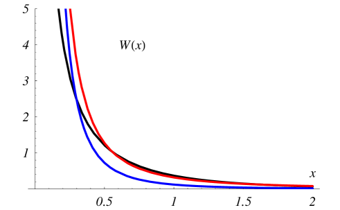
Figure 1: Densities $W(x)$ of the Lévy measures for the selfdecomposable laws $\mathcal{L}(a)$ (black), $\mathcal{C}(a)$ (red) and $\mathcal{S}(a)$ (blue). To make the plots comparable we have chosen $a=1$ for all the three densities, and to make the differences more visible we have plotted only the positive $x$–axis since the curves are exactly symmetric on the negative axis.

Examples of these three densities are plotted in Figure 1.

4.2 Convergence of consecutive sums

To give examples of consecutive sums converging to our laws let us first of all recall what happens in the case of the Poisson laws $\mathcal{P}(\lambda)$. Let $\mathcal{B}(n,p)$ represent the binomial laws for $n$ independent trials of verification of an event occurring with probability $p$, and take the triangular array of Bernoulli 0–1 random variables $X_{k}^{(n)}\sim\mathcal{B}(1,\lambda/n)$ with $k=1,\ldots,n$ and $n=1,2,\ldots\,$ Apparently they are uniformly, asymptotically negligible because for $0<\epsilon<1$ we have

$$\max_{k}\,\mathbf{P}\left\{{|X_{k}^{(n)}|\geq\epsilon}\right\}=\frac{\lambda}{n}\stackrel{{\scriptstyle n}}{{\longrightarrow}}0\,.$$

It is very well known that the consecutive sums are Binomial random variables, namely

$$S_{n}=X_{1}^{(n)}+\ldots+X_{n}^{(n)}\sim\mathcal{B}\left(n,\frac{\lambda}{n}\right)$$

and that, according to the classical Poisson theorem, the limit law of these $S_{n}$ is $\mathcal{P}(\lambda)$. Remark that, since in passing from $n$ to $n^{\prime}$ the random variables $X_{k}^{(n)}$ change type, it will not be possible to put $S_{n}$ in the form of a normed sum as (4). The Poisson laws, however, are also limit laws in a still legitimate, but rather trivial sense due to the composition properties of the family $\mathcal{P}(\lambda)$: take for instance a triangular array of Poisson random variables $X_{k}^{(n)}\sim\mathcal{P}(\lambda/n)$ with $k=1,\ldots,n$ and $n=1,2,\ldots\,$ which are again uniformly, asymptotically negligible because for $0<\epsilon<1$ we have

$$\max_{k}\,\mathbf{P}\left\{{|X_{k}^{(n)}|\geq\epsilon}\right\}=1-e^{-\lambda/n}\stackrel{{\scriptstyle n}}{{\longrightarrow}}0\,.$$

Now – at variance with the previous example of the Bernoulli triangular array – at every step $n$ we exactly have $S_{n}\sim\mathcal{P}(\lambda)$ and hence, albeit in a trivial sense, the limit law again is $\mathcal{P}(\lambda)$. Also in this case $X_{k}^{(n)}$ and $X_{k}^{(n^{\prime})}$ belong to different types, so that it will be impossible to put $S_{n}$ in the form of a normed sum as (4). Of course both these examples show in what sense the Poisson laws are infinitely divisible but not selfdecomposable: they are limit laws of consecutive sums (2) of uniformly, asymptotically negligible triangular arrays, but not of normed sums (4) of independent random variables.

At the other end of the gamut of the infinitely divisible laws we find the 2–stable normal laws. To see in what sense they are limit laws take an arbitrary sequence $X_{k}$ of centered, independent and identically distributed random variables with finite variance $\sigma^{2}$ and define the triangular array

$$X_{k}^{(n)}=\frac{X_{k}}{\sigma\sqrt{n}}$$

which always turns out to be uniformly, asymptotically negligible because of the Chebyshev inequality:

$$\max_{k}\,\mathbf{P}\left\{{|X_{k}^{(n)}|\geq\epsilon}\right\}=\max_{k}\,\mathbf{P}\left\{{|X_{k}|\geq\epsilon\sigma\sqrt{n}}\right\}\leq\frac{1}{\epsilon^{2}n}\stackrel{{\scriptstyle n}}{{\longrightarrow}}0\,.$$

The consecutive sums are now also normed sums of independent and identically distributed random variables since

$$S_{n}=X_{1}^{(n)}+\ldots+X_{n}^{(n)}=\frac{1}{\sigma\sqrt{n}}\sum_{k=1}^{n}X_{k}$$

and according to the classical, normal Central Limit Theorem their limit law is $\mathcal{N}(1)$. Also in this case, however, it is possible to exploit the composition properties of the normal type to find another, more trivial form of the consecutive sums: take the sequence of normal independent and identically distributed random variables $X_{k}\sim\mathcal{N}(1)$ and define the triangular array $X_{k}^{(n)}=X_{k}/\sqrt{n}\sim\mathcal{N}(1/n)$ which again apparently is uniformly, asymptotically negligible. Now the consecutive sums are also normed sums which – at variance with the previous example – are all normally distributed

$$S_{n}=X_{1}^{(n)}+\ldots+X_{n}^{(n)}=\frac{1}{\sqrt{n}}\sum_{k=1}^{n}X_{k}\sim\mathcal{N}(1)$$

and hence, in a trivial sense, the limit law is $\mathcal{N}(1)$. Finally let us remark that, since the normal laws are infinitely divisible, nothing will forbid them to be also limit laws of consecutive sums of triangular arrays that do not reduce to normed sums of independent and identically distributed random variables. However we will not elaborate here examples in this sense.

We have introduced the trivial forms of the consecutive sums in the case of the Poisson and normal laws (see also the remarks at the end of the Section 2.1) only because in our other subsequent examples this will be the unique explicit form available for our $S_{n}$. Remark also that these trivial forms essentially derive from the fact that our laws are all infinitely divisible. In fact if $\varphi$ is infinitely divisible, then also $\varphi_{n}=\varphi^{1/n}$ is a characteristic function, and of course $\varphi_{n}^{n}=\varphi$ for every $n$. In general – with the exception of the stable laws – the $\varphi_{n}$ are not of the same type for different $n$, and hence the sums can not take the form of normed sums. That notwithstanding, in a trivial sense, every infinitely divisible law $\varphi$ is the limit law of the consecutive sums of independent and identically distributed random variables all distributed according to $\varphi_{n}$. What is less trivial, however, is to give an explicit form to the cumulative distribution function or density function of the component laws $\varphi_{n}$: as the subsequent examples will show this can be easily done only when we deal with families of laws closed under composition and decomposition.

Let us consider first the Cauchy laws introduced in the previous Section 4.1: they are 1–stable and, by taking advantage of the fact that the family $\mathcal{C}(a)$ is closed under composition and decomposition, it will be easy to show how they are limit laws of suitable sums of random variables. Take for instance a sequence of independent and identically distributed Cauchy random variables $X_{k}\sim\mathcal{C}(a)$ and define the triangular array $X_{k}^{(n)}=X_{k}/n\sim\mathcal{C}(a/n)$. Since now there is no variance to speak about, to show that this sequence is uniformly, asymptotically negligible we can not use the Chebyshev inequality. If however

$$F(x)=\frac{1}{2}+\frac{1}{\pi}\arctan\frac{x}{a}$$

is the common cumulative distribution function of the $X_{k}$, it is easy to see that the sequence is uniformly, asymptotically negligible because

$$\max_{k}\,\mathbf{P}\left\{{|X_{k}^{(n)}|\geq\epsilon}\right\}=\max_{k}\,\mathbf{P}\left\{{|X_{k}|\geq\epsilon n}\right\}=2\left[1-F(\epsilon n)\right]\stackrel{{\scriptstyle n}}{{\longrightarrow}}0\,.$$

Now, as for the Gaussian case, the consecutive sums are also normed sums of independent and identically distributed random variables and are all distributed according to the Cauchy law $\mathcal{C}(a)$

$$S_{n}=X_{1}^{(n)}+\ldots+X_{n}^{(n)}=\frac{1}{n}\sum_{k=1}^{n}X_{k}\sim\mathcal{C}(a)$$

so that, in a trivial sense, the limit law is $\mathcal{C}(a)$. What forbids here the convergence to the normal law is the fact that the variance is not finite, so that the normal Central Limit Theorem does not apply. At variance with the Poisson and Gaussian previous examples, however, we do not know non trivial forms of a Cauchy limit theorem embodying the stability of the Cauchy law. In other words we have neither explicit examples, nor general theorems characterizing the form of the normed sums of independent and identically distributed random variables whose laws converge to $\mathcal{C}(a)$, without being coincident with $\mathcal{C}(a)$ at every step $n$ of the limiting process.

This last remark holds also in the case of the Laplace selfdecomposable, but not stable laws $\mathcal{L}(a)$. In fact, since the $\mathcal{VG}(\lambda,a)$ family is closed under composition and decomposition, we can always take a triangular array $X_{k}^{(n)}\sim\mathcal{VG}(1/n,\,a)$ for $k=1,\ldots,n$ and $n=1,2,\ldots$, and remark first that they are uniformly, asymptotically negligible by virtue of the Chebyshev inequality (the $X_{k}^{(n)}$ have finite variance $2a^{2}/n\stackrel{{\scriptstyle n}}{{\longrightarrow}}0$), and then that for every $n$

$$S_{n}=X_{1}^{(n)}+\ldots+X_{n}^{(n)}\sim\mathcal{VG}(1,a)=\mathcal{L}(a)$$

so that the limit law trivially is $\mathcal{L}(a)$. It must also be said that in this example the random variables of the triangular array change type with $n$ so that the corresponding consecutive sums $S_{n}$ can not be recast in the form of normed sums of independent random variables. Since however the Laplace laws are not only infinitely divisible, but also selfdecomposable we would expect to find normed sums of independent (albeit not identically distributed, because the Laplace laws are not stable) random variables whose laws converge to $\mathcal{L}(a)$. Unfortunately we do not have general theorems characterizing the needed sequences of independent random variables, and we can just show an example slightly more general than the previous one. Take for instance the triangular array $X_{k}^{(n)}$ with laws $\mathcal{VG}\left(\frac{1}{k(2+\log n)}\,,a\right)$ and variances $\frac{a^{2}}{k(2+\log n)}$. They are uniformly, asymptotically negligible because from the Chebyshev inequality we have

$$\max_{k}\,\mathbf{P}\left\{{|X_{k}^{(n)}|\geq\epsilon}\right\}\leq\max_{k}\,\frac{a^{2}}{\epsilon^{2}k(2+\log n)}=\frac{a^{2}}{\epsilon^{2}(2+\log n)}\stackrel{{\scriptstyle n}}{{\longrightarrow}}0\,,$$

while, for a known property of the harmonic numbers, the consecutive sums are

$$S_{n}=X_{1}^{(n)}+\ldots+X_{n}^{(n)}\sim\mathcal{VG}\left(\frac{1}{2+\log n}\sum_{k=1}^{n}\frac{1}{k}\,,\,a\right)\stackrel{{\scriptstyle n}}{{\longrightarrow}}\mathcal{L}(a)\,.$$

Now the sums $S_{n}$ are not trivially distributed according to $\mathcal{L}(a)$ at every $n$, but again they can not be put in the form of normed sums as they should since $\mathcal{L}(a)$ is selfdecomposable.

Finally similar remarks can be done for the selfdecomposable, but not stable Student laws $\mathcal{S}(a)$ introduced in the Section 4.1, but in this last case it is not even possible to give a simple form to the trivial consecutive sums because the Student family $T(\lambda,a)$ is not closed under composition and decomposition. In other words if $\varphi$ is the characteristic function of a law $\mathcal{S}(a)$ we are sure that $\varphi_{n}=\varphi^{1/n}$ again is the characteristic function of a infinitely divisible law such that $\varphi_{n}^{n}=\varphi$ for every $n$, but these component laws $\varphi_{n}$ no longer belong to the $T(\lambda,a)$ family as happens for the Variance–Gamma family, and in fact the form for their density function is rather complicated [10].

4.3 Stationary and selfsimilar processes

Since all the laws of our examples are infinitely divisible we can use all of them to generate the corresponding Lévy processes by using (12) to give the law of the increments on a time interval of width $t$. In particular we will explicitly do that for the laws $\mathcal{N}(a)$, $\mathcal{L}(a)$, $\mathcal{C}(a)$ and $\mathcal{S}(a)$. We then get as stationary increment characteristic functions $\phi_{t}(u)$ respectively

$$e^{-a^{2}tu^{2}/2T}\qquad\qquad\qquad\qquad\;\;\,\hbox{{Wiener process} from $\mathcal{N}(a)$}$$

$$\left(1+a^{2}u^{2}\right)^{-t/T}\qquad\qquad\qquad\;\,\hbox{{Laplace process} from $\mathcal{L}(a)$}$$

$$e^{-at|u|/T}\qquad\qquad\qquad\qquad\quad\;\>\hbox{{Cauchy process} from $\mathcal{C}(a)$}$$

$$e^{-at|u|/T}(1+a|u|)^{t/T}\qquad\qquad\hbox{{Student process} from $\mathcal{S}(a)$}$$

It is then apparent that the laws of the increments for the $\alpha$–stable Wiener and Cauchy processes are simply $\mathcal{N}(a\sqrt{t/T})$ and $\mathcal{C}(at/T)$, while for the Laplace process the law of the increments is actually a Laplace law only for $t=T$, while in general it is a $\mathcal{VG}(t/T,a)$ at other values of $t$. For our Student process, on the other hand, the situation is less simple because the Student family is not closed under convolution, and the increment law no longer is in $T(\lambda,a)$ for $t\neq T$. In this case it is not easy to find the actual distribution from its Fourier transform $\phi_{t}(u)$, and only recently it has been suggested that the increments are distributed according to a mixture of other Student laws (for further details see [10]). The Wiener and the Cauchy processes are $H$–selfsimilar with $H=1/2$ and $H=1$ respectively. This can also be seen by looking at the interplay between the two – spatial and temporal – scale parameters $a$ and $T$. In fact in the Wiener and Cauchy processes these two scale parameters appear in two combinations – respectively $a^{2}/T$ and $a/T$ – such that a change in the time units can always be compensated by a corresponding, suitable change in the space units; as a consequence the distribution of the process is left unchanged by these twin scale changes. This, on the other hand, would not be possible in the Laplace and Student processes since $a$ and $T$ no longer appear in such combinations.

That notwithstanding we can achieve selfsimilarity in additive, non stationary processes produced by all our selfdecomposable laws. From (15) in fact we can give the characteristic function $\phi_{s,t}(u)$ of the increments in the interval $[s,t]$ for our four types of law. First of all from the Normal type $\mathcal{N}(a)$ we get

$$\phi_{s,t}(u)=e^{-a^{2}\left(t^{2H}-s^{2H}\right)u^{2}/2T^{2H}}$$

namely

$$X(t)-X(s)\sim\mathcal{N}\left(a^{2}\,\frac{t^{2H}-s^{2H}}{T^{2H}}\right)\,.$$

These laws define processes which coincide with the usual Wiener process if and only if $H=1/2$. For $H\neq 1/2$, on the other hand, our process is additive, $H$–selfsimilar, and Gaussian with non stationary increments, and hence does not even coincide with a fractional Brownian motion which has stationary and correlated increments. In a similar way from the laws of the Cauchy type $\mathcal{C}(a)$ we get

$$X(t)-X(s)\sim\mathcal{C}\left(a\,\frac{t^{H}-s^{H}}{T^{H}}\right)\,,$$

and the process will coincide with the stationary (Lévy) Cauchy process when $H=1$, while for $H\neq 1$ we have an additive, $H$–selfsimilar process with non stationary increments. From the Laplace type $\mathcal{L}(a)$ on the other hand we obtain an $H$–selfsimilar (with $H>0$), additive process when we take

$$\phi_{s,t}(u)=\frac{1+a^{2}\left(\frac{s}{T}\right)^{2H}u^{2}}{1+a^{2}\left(\frac{t}{T}\right)^{2H}u^{2}}\>=\>\left(\frac{s}{t}\right)^{2H}+\left[1-\left(\frac{s}{t}\right)^{2H}\right]\frac{1}{1+a^{2}\left(\frac{t}{T}\right)^{2H}u^{2}}\,;$$

so that, for $s>0$, the law of the increment on an interval $[s,t]$ actually is a mixture – with time–dependent probabilistic weights – of a law degenerate in $x=0$ and of a Laplace law:

$$X(t)-X(s)\sim\left(\frac{s}{t}\right)^{2H}\delta_{0}+\left[1-\left(\frac{s}{t}\right)^{2H}\right]\mathcal{L}\left(\frac{a^{2}t^{2H}}{T^{2H}}\right)\,.$$

In other words this means that for $s>0$ there is always a non–zero probability that in $[s,t]$ the process increment will simply vanish. Finally from the Student type $\mathcal{S}(a)$ we get the additive, $H$–selfsimilar, non stationary process with

$$\phi_{s,t}(u)=\frac{e^{-at^{H}|u|/T^{H}}\left(1+\frac{at^{H}}{T^{H}}|u|\right)}{e^{-as^{H}|u|/T^{H}}\left(1+\frac{as^{H}}{T^{H}}|u|\right)}\,,$$

so that $X(t)\sim\mathcal{S}\left(at^{H}/T^{H}\right)$, while nothing simple enough can be said of the independent increment laws.

4.4 Ornstein–Uhlenbeck stationary distributions

All the Lévy processes introduced in the Section 4.3 can now be used as driving noises of Ornstein–Uhlenbeck processes according to the discussion of the Section 3.3. Here we will only list the essential properties of the corresponding stationary distributions by analyzing their logarithmic characteristics (18). First of all, if $b$ is the parameter of the process as in (16) (remember that we took there $T=1$ for simplicity), for the Wiener and the Cauchy driving noises we immediately have from (18) that the logarithmic characteristics $\psi(u)$ of the stationary distributions are respectively

$$-\frac{a^{2}u^{2}}{4b}\,,\qquad\qquad\quad\hbox{for a Wiener noise (usual Ornstein--Uhlenbeck\ process)}$$

$$-\frac{a|u|}{b}\,,\qquad\qquad\quad\;\hbox{for a Cauchy noise}$$

namely that the stationary distributions simply are $\mathcal{N}(a/\sqrt{2b})$ and $\mathcal{C}(a/b)$. In the case of the Wiener noise (namely in the case of the ordinary, Gaussian Ornstein–Uhlenbeck process) this means that the stationary distribution has a variance $a^{2}/2b$ while the Gaussian law generating the Wiener process had a variance $a^{2}$. For the Cauchy noise, on the other hand, there is no variance to speak about.

For the other two Ornstein–Uhlenbeck Lévy noises (Laplace and Student) an important role is played by the so called dilogarithm function [14, 15, 16]

$$\mathrm{Li}_{2}(x)=\int_{x}^{0}\frac{\log(1-s)}{s}\,ds\,,\qquad\left(=\sum_{k=1}^{\infty}\frac{x^{k}}{k^{2}}\,,\qquad|x|\leq 1\right)$$

In fact a direct calculation of the integrals (18) gives for the logarithmic characteristics $\psi(u)$

$$\frac{1}{2b}\,\mathrm{Li}_{2}(-a^{2}u^{2})\,,\qquad\qquad\qquad\qquad\;\hbox{for a Laplace noise}$$

$$-\frac{a|u|}{b}-\frac{1}{b}\,\mathrm{Li}_{2}(-a|u|)\,,\qquad\qquad\quad\;\hbox{for a Student noise}$$

From the characteristic functions $\varphi(u)=e^{\psi(u)}$ we can also calculate the stationary variances as $-\varphi^{\prime\prime}(0)$ and we get $a^{2}/b$ and $a^{2}/2b$ respectively in the Laplace and in the Student case. Remark that – when they exist finite – the variances of the stationary distributions always are in the same relation with the variance of the law generating the noise: the stationary variance is the generating law variance divided by $2b$. The form of the corresponding density functions is not known analytically, but it can be assessed by numerically calculating the inverse Fourier transforms of the characteristic functions: the results of these calculations for a couple of particular cases are shown in the Figures 3 and 3.

Finally, since the types of laws analyzed in this section are all selfdecomposable, by reversing the previous procedure we can also add a few remarks about the Ornstein–Uhlenbeck driving noises required to have $\mathcal{N}(a)$, $\mathcal{L}(a)$, $\mathcal{C}(a)$ and $\mathcal{S}(a)$ as stationary distributions. In fact we have already said that for our two $\alpha$–stable cases the stationary distributions are of the same type of the laws generating the driving noise, so that there is essentially nothing to add for the $\mathcal{N}(a)$ and $\mathcal{C}(a)$ stationary distributions. As for the other two cases on the other hand we will use the second equation (18) to calculate the noise logarithmic characteristics $\chi(u)$:

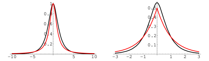
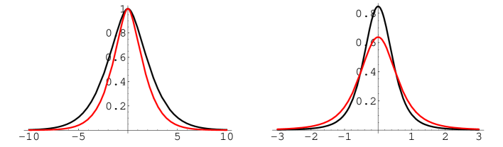
Figure 2: Ornstein–Uhlenbeck process driven by a Laplace noise: characteristic functions (left) and density functions (right) of the stationary distribution (black lines), compared with the characteristic functions and density functions of the Laplace law $\mathcal{L}(a)$ generating the driving noise (red lines). Here $a=1/\sqrt{2}$ and $b=1$ so that both the variances (that of the stationary distribution, and that of $\mathcal{L}(a)$) are equal to 1.

Figure 3: Ornstein–Uhlenbeck process driven by a Student noise: characteristic functions (left) and density functions (right) of the stationary distribution (black lines), compared with the characteristic functions and density functions of the Student law $\mathcal{S}(a)$ generating the driving noise (red lines). Here $a=b=1$ so that both the variances (that of the stationary distribution, and that of $\mathcal{S}(a)$) are equal to 1.

$$-2b\,\frac{a^{2}u^{2}}{1+a^{2}u^{2}}\,,\qquad\qquad\qquad\qquad\>\hbox{for a Laplace $\mathcal{L}(a)$ stationary law}$$

$$-b\,\frac{a^{2}u^{2}}{1+a|u|}\,,\qquad\qquad\qquad\qquad\quad\hbox{for a Student $\mathcal{S}(a)$ stationary law}$$

In both cases however the characteristic functions can not be elementarily inverted so that we do not have an explicit expression for the increment density functions of the the Lévy noises that produce these two stationary Ornstein–Uhlenbeck distributions. We can only add a few remarks about the Laplace case: here the characteristic function $\varphi(u)=e^{\psi(u)}$ does not vanish at the infinity since $\varphi(\pm\infty)=e^{-2b}$. As a consequence the Lévy noise increment characteristic function can be better written as

$$[\varphi(u)]^{t}=e^{-2bta^{2}u^{2}/(1+a^{2}u^{2})}=e^{-2bt}+(1-e^{-2bt})\,\frac{e^{2bt/(1+a^{2}u^{2})}-1}{e^{2bt}-1}$$

so that the independent increments of an Ornstein–Uhlenbeck process with the Laplace type $\mathcal{L}(a)$ as stationary law are distributed according to a time–dependent mixture of two laws, one of which is degenerate in $x=0$. As for the second law of this mixture, it has a density function given by

$$f(x,t)=\frac{1}{\pi}\int_{0}^{+\infty}\cos(ux)\,\frac{e^{2bt/(1+a^{2}u^{2})}-1}{e^{2bt}-1}\,\,du$$

but this integration can not be analytically performed.

5 Conclusions

Since many years selfsimilarity is a fashionable subject of investigation, in areas ranging from fractals to long–range interactions in complex systems: to have an idea just ask for the papers with the word “self similarity” either in their title or in their abstract present on arxiv.org and you will find $1\,000$ articles, and almost 200 of them only in the first six months of 2007. On the other hand this is a subject that has been approached from many different standpoints producing an unavoidable level of confusion [1], while in fact it would be better discussed by placing the reader in the perspective of the general theory of the infinitely divisible (even non stable) processes. In the field of mathematical finance the use of non stable Lévy processes is widespread, and several families of selfdecomposable laws and processes have been intensively studied in recent years: see for example the case of the Generalized Hyperbolic family [17, 18, 19], of the Student family [10, 20], and of the Variance Gamma family [21, 22, 23, 24]. Considerable interest has also been elicited by the use of selfdecomposable laws in connection with the Ornstein–Uhlenbeck processes [7, 9], in particular for the stochastic volatility modelling. However, while in econophysics some non stable Lévy laws are recognized as possible candidates for a consistent modelling of the underlying processes [25, 26], they remain less popular in the field of statistical mechanics and only recently their use has been proposed in connection with applications to the technology of accelerator beams [10, 27, 28]

In this paper we have tried to elucidate just a few points in the framework of the theory of stochastic processes. In particular we focused our attention on the relation between on the one hand the selfsimilarity, and on the other the independence and the stationarity of the increments. This has led our inquiry toward the analysis of the laws of the process increments, and we have stressed the connection between the selfsimilarity of the process and the selfdecomposability of the increment laws. Selfdecomposable laws naturally arise in the study of the Central Limit Problem and of its solutions: in fact they are an intermediate (and more elusive) class of distributions between the more general infinitely divisible, and the more particular (and more popular) stable distributions. We found then that, in the case of selfdecomposable generating laws, both the stationarity of the increments and the selfsimilarity are always possible, but are not always present in the same process. On the other hand selfsimilarity can also be a property of (non Markovian) processes with non independent increments as in the case of the fractional Brownian motion. We finally stressed the connection between the selfdecomposability and the stationary laws of generalized Ornstein–Uhlenbeck processes with non Gaussian, Lévy noises. All that has also be elucidated by means of a few particular examples, and some kind of application from physics to finance has also been pointed out.

References

- [1] J L McCauley, G H Gunaratne and K A Bassler Hurst exponent, Markov processes and Fractional Brownian motion in press on Physica A (2007)
- [2] M Loève, Probability Theory I (Springer, 1977)
- [3] M Loève, Probability Theory II (Springer, 1978)
- [4] B V Gnedenko and A N Kolmogorov, Limit distributions for sums of independent random variables (Addison–Wesley, 1968)
- [5] K Sato, Lévy processes and infinitely divisible distributions (Cambridge University Press, 1999)
- [6] A N Shiryayev, Probability (Springer, 1984)
- [7] R Cont and P Tankov, Financial modelling with jump processes (Chapman&Hall/CRC, 2004)
- [8] K Sato, Probab Th Rel Fields 89 (1991) 285.
- [9] P Carr, H Geman, D B Madan and M Yor, Math Fin 17 (2007) 31
-
[10]
N Cufaro Petroni, J Phys A 40 (2007)
2227, also available as
math.PR/0702058athttp://arxiv.org/ - [11] B B Mandelbrot and J W Van Ness, SIAM Rev 10 (1968) 422
-
[12]
Y Hu and B Øksendal, Fractional white noise
calculus and applications to finance, preprint 10/1999 in Pure
Mathematics of the Department of Mathematics of the Oslo University;
available at
http://www.math.uio.no/eprint/pure_math/1999/10-99.html - [13] Ph E Protter, Stochastic integration and differential equations (Springer, 2005)
- [14] M Abramowitz and I A Stegun Handbook of Mathematical Functions (Dover Publications, 1968)
- [15] L Lewin Dilogarithms and associated functions (McDonald, 1958)
- [16] R Morris Math. Comp. 33 (1979) 778
- [17] E Eberlein and S Raible European Congress of Mathematics (Barcelona) vol II (Progress in Mathematics vol 202) ed C Casacuberta et al (Basel, Birkhäuser 2000) p 367.
- [18] S Raible Lévy processes in finance: theory, numerics and empirical facts, PhD Thesis (Freiburg University 2000).
- [19] E Eberlein in Lévy processes, Theory and applications ed Barndorff–Nielsen O et al (Boston, Birkhäuser 2001) p 371.
- [20] C C Heyde and N N Leonenko Adv. Appl. Prob. 37 (2005) 342.
- [21] D B Madan and E Seneta Journal of the Royal Statistical Society series B 49(2) (1987) 163.
- [22] D B Madan and E Seneta Journal of Business 63 (1990) 511.
- [23] D B Madan and F Milne Mathematical Finance 1(4) (1991) 39.
- [24] D BMadan , P P Carr and E C Chang European Finance Review 2 (1998) 79.
- [25] J–Ph Bouchaud and M Potters Theory of financial risks: from statistical physics to risk management (Cambridge, Cambridge University Press 2000)
- [26] R Mantegna and H E Stanley An introduction to econophysics (Cambridge, Cambridge University Press 2001)
- [27] N Cufaro Petroni, S De Martino, S De Siena and F Illuminati Phys Rev E 72 (2005) 066502
- [28] N Cufaro Petroni, S De Martino, S De Siena and F Illuminati Nucl Instrum Methods A 561 (2006) 237