Flipped spinfoam vertex and loop gravity
Abstract
We introduce a vertex amplitude for 4d loop quantum gravity. We derive it from a conventional quantization of a Regge discretization of euclidean general relativity. This yields a spinfoam sum that corrects some difficulties of the Barrett-Crane theory. The second class simplicity constraints are imposed weakly, and not strongly as in Barrett-Crane theory. Thanks to a flip in the quantum algebra, the boundary states turn out to match those of loop quantum gravity – the two can be identified as eigenstates of the same physical quantities – providing a solution to the problem of connecting the covariant spinfoam formalism with the canonical spin-network one. The vertex amplitude is and -covariant. It rectifies the triviality of the intertwiner dependence of the Barrett-Crane vertex, which is responsible for its failure to yield the correct propagator tensorial structure. The construction provides also an independent derivation of the kinematics of loop quantum gravity and of the result that geometry is quantized.
1 Introduction
While the kinematics of loop quantum gravity (LQG) [1] is rather well understood [2, 3], its dynamics is not understood as cleanly. Dynamics is studied along two lines: hamiltonian [4] or covariant. The key object that defines the dynamics in the covariant language is the vertex amplitude, like the vertex amplitude that defines the dynamics of perturbative QED. What is the vertex of LQG?
The spinfoam formalism [5, 6, 7, 8, 9] can be viewed as a tool for answering this question: the spinfoam vertex plays a role similar to the vertices of Feynman’s covariant quantum field theory. This picture is nicely implemented in three dimensions (3d) by the Ponzano-Regge model [10], whose boundary states match those of LQG [11] and whose vertex amplitude can be obtained as a matrix element of the hamiltonian of 3d LQG [12]. But the picture has never been fully implemented in 4d. The best studied model in the 4d euclidean context is the Barrett-Crane (BC) theory [8], which is based on the vertex amplitude introduced by Barrett and Crane [7]. This is simple and elegant, has remarkable finiteness properties [13], but the suspicion that something is wrong with it has long been agitated. Its boundary state space is similar to, but does not exactly match, that of LQG; in particular the volume operator is ill-defined. Worse, recent results [14] indicate that it appear to fail to yield the correct tensorial structure of the graviton propagator in the low-energy limit [15].
It is then natural to try to correct the BC model [16, 17, 18]. The difficulties are all related to the fact that in the BC model the intertwiner quantum numbers are fully constrained. This follows from the fact that the simplicity constraints are imposed as strong operator equations (). However, these constraints are second class and it is well known that imposing second class constraints strongly may lead to the incorrect elimination of physical degrees of freedom [19]. In this paper we show that the simplicity constraints can be imposed weakly (), and that the resulting theory has remarkable features. First, its boundary quantum state space matches exactly the one of LQG: no degrees of freedom are lost. Second, as the degrees of freedom missing in BC are recovered, the vertex may yield the correct low-energy -point functions. Third, the vertex can be seen as a vertex over spin networks or spin networks, and is both and covariant.
These results have been anticipated in a letter [20]. Here we derive them via a proper quantization of a discretization of euclidean general relativity (GR). Indeed, although spinfoam models have been derived in a number of different manners [6, 7, 8, 21], most derivations involve peculiar procedures or intuitive and ad hoc steps. It is hard to find a proper derivation of a spinfoam model from the classical field theory, which follows well-tested quantization procedures. Here we try to fill this gap.
From the experience with QCD, one can derive the persuasion that a nontrivial quantum field theory should be related to a natural lattice discretization of the corresponding classical field theory [22]. This persuasion is reinforced by the LQG prediction of an actual physical discretization of spacetime. Here, we reconstruct the basis of the euclidean spinfoam formalism as a proper quantization of a lattice discretization of GR. Conventional lattice formalisms as the ones used in QCD are not very natural for GR, since they presuppose a background metric. Regge has found a particularly natural way to discretize GR on a lattice [23], known as Regge calculus. Quantization of Regge calculus has been considered in the past [24] and its relation to spinfoam theory has been pointed out (see [25] and references therein). Here we express Regge calculus in terms of the elementary fields used in the loop and spinfoam approach, namely holonomies and the Plebanski two-form, and we study the quantization of the resulting discrete theory (on lattice derivations of loop gravity, see [6, 27, 28]).
The technical ingredient that allows a nontrivial intertwiner state space to emerge can be interpreted as a “flip” of the algebra, namely an opposite choice of sign in one of its two factors. The possibility and the relevance of a “flipped” symplectic structure was noticed by Baez and Barrett in [26] (where they attribute the observation to José-Antonio Zapata) and by Montesinos [29]. Montesinos, in particular, has discussed the classical indeterminacy of the symplectic structure in detail. The flip can be viewed as the equivalent of the Ashtekar “trick”, which yields a connection as phase space variable. The generators turn out to directly correspond to the bivectors associated to the Regge triangles, rather than to their dual. Using this, we find a nontrivial subspace of the intertwiner space, which corresponds to closed tetrahedra and maps naturally to an intertwiner space.
This path leads to a quantum theory that appears to improve several aspects of the better known spinfoam models. In particular: (i) the geometrical interpretation for all the variables becomes fully transparent; (ii) the boundary states fully capture the gravitational field boundary variables; and (iii) correspond precisely to the spin network states of LQG. The identification is not arbitrary: the boundary states of the model are precisely eigenstates of the same quantities as the corresponding LQG states. This last result provides a solution to the long-standing difficulty of connecting the covariant spinfoam formalism with the canonical LQG one. It also provides a novel independent derivation of the LQG kinematics, and, in particular, of the quantization of area and volume. Finally, (iv) the vertex of the theory is similar to, but different from, the BC vertex, leading to a dynamics that might be better behaved in the low-energy limit.
The paper is organized pedagogically and is largely self contained. Section 2 reviews background material: properties of and its selfdual/anti-selfdual split, and the definition of the fields and the formulation of classical GR as a constrained Plebanski theory. In section 3 we discretize the theory on a fixed triangulation of spacetime. We do so simply by taking standard Regge calculus and re-expressing it in terms of the (discretized) Plebanski two-form. The resulting theory is governed by the geometry of a 4-simplex, which we illustrate in detail. All basic relations among the variables have a simple interpretation in these terms. The 10 components of the metric tensor in a point (or in a cell) can be interpreted as a way to code the 10 variables determining the shape of the cell. In particular, the norms of the discretized fields on the faces are their areas and the scalar product on adjacent triangles codes the angle between the triangles. While these “angles” and “areas” are independent in BF theory, they are related if they derive from a common metric, namely in GR. In Section 4 we study the quantization of the system. We explain the difficulties of imposing the constraints strongly, study the weak constraints and write their solution. Finally we construct the vertex amplitude.
We work in the euclidean signature, and on a fixed triangulation. The issues raised by recovering triangulation independence and the relation with the Lorentzian–signature theory will be discussed elsewhere.
2 Preliminaries: Plebanski two-form and structure of
Riemannian general relativity (GR) is defined by a riemannian metric , where and the Einstein-Hilbert action
| (1) |
where is the inverse, the determinant, and the Ricci curvature of . A good number of reasons, such as for instance the fact that this metric formulation is incompatible with the coupling with fermions, suggest to use the tetrad field , (the value 0 instead of 4 is for later convenience and does not indicate a Lorentzian metric) or its inverse, namely the tetrad one-form field , to describe the gravitational field. This is related to the metric by . Sum over repeated indices is understood, and the up or down position of the indices is irrelevant. The spin connection of the tetrad field is an connection satisfying the torsion-free condition
| (2) |
The action (1) can be rewritten as a function of in the form
| (3) |
where is the curvature of . Alternatively, GR can be defined in first order form in terms of independent variables and , by the action
| (4) |
In this case, (2) is obtained as the equation of motion for .
2.1 Plebanski two-form and simplicity constraints
At the basis of the spinfoam formalism is the use of the Plebanski two-form , defined as
| (5) |
or its dual, usually called for a reason that will be clear in a moment, defined as
| (6) |
We use the following notation for two-index objects: a scalar product: ; a norm: , and the duality operation . So that, in particular, . Thus we write (6) in the form
| (7) |
The geometrical interpretation of the Plebanski two-form (or the two-form) is captured by the following. Observe that
| (8) |
and
| (9) |
The quantity gives the area element of the infinitesimal surface . Therefore we can write
| (10) |
The quantity is the related to the angle between the surface elements and . In fact, if we take the scalar product of the normals of these two surface elements (in the 3-space they span), we obtain (without writing the infinitesimals vectors)
| (11) |
Finally, the 4-form
| (12) |
is easily seen to be (proportional to) the volume element . Intuitively, describing the geometry in terms of rather than is using as elementary variable areas and angles rather than length and angles.
Using the Plebanski field, the action can be written in the BF-like form
| (13) |
The reason this action defines GR and not BF theory is that the independent variable to vary is the tetrad , not the two-form . While the BF field equations are obtained by varying the action (13) under arbitrary variations of (and ), GR is defined by varying this action under the variations that respect the form (6) of the field . This condition can be expressed as a constraint equation for :
| (14) |
Equivalently ,
| (15) |
where . This system of constraint can be decomposed in three parts:
| (16) | |||||
| (17) | |||||
| (18) |
where the indices are all different, and the sign in the last equation is determined by the sign of their permutation. Equivalently, the field satisfies these same equations. These three constraint play an important role in the following. They are called the simplicity constraints. GR can be written as an BF theory whose field satisfies the simplicity constraints (16-17-18).
2.2 Selfdual structure of
In this section we recall some elementary facts about and we make an observation about its representations that plays a role in the following.
The group is locally isomorphic to the product of two subgroups, each loc. isomorphic to : . That is, we can write each in the form where and and . This is clearly seen looking at its algebra , which is the linear sum of two commuting algebras. Explicitly, let be the generators of . Define the selfdual and anti-selfdual generators that satisfy . Then it is immediate to see that . The span a three dimensional subalgebra of , and the span a three dimensional subalgebra of , both isomorphic to .
It is convenient to choose a basis in and in . For this, choose a unit norm vector in , and three other vectors forming, together with , an orthonormal basis, for instance , and define
| (19) |
The structure is then easy to see, since . In particular, we can choose , and , and we have
| (20) |
Notice that in choosing this basis we have broken invariance. In fact, the split is canonical, but there is no canonical isomorphism between and or between and . One such isomorphism is picked up, for instance, by choosing the vector . It sends to , where the element of leaves invariant. This isomorphism defines a notion of diagonal elements of the algebra: the ones of the form . Exponentiating these, we get the diagonal elements of the group, which we can write as . These diagonal elements form an subgroup of , which is not canonical: it depends on . It is the subgroup of that leaves the vector invariant. If we consider the 3d surface (“space”) orthogonal to , the diagonal part of is (the double covering of) the group of the (“spatial”) rotations of this space; we denote it . Borrowing from the Lorentzian terminology, we can call “boost” a change of . Its effect is to rotate the bases relative to one another.
Notice that for any two-index quantity ,
| (21) |
while
| (22) |
This split is independent from , as the norms are not affected by a rotation of the basis. In particular, and are the scalar and pseudo-scalar quadratic Casimirs of . They are, respectively, the sum and the difference of the quadratic Casimirs of and . The representations of the universal cover of , the group are labelled by two half integers . The representations of form the subset of these for which is integer. The representations satisfying , which clearly belong to this subset, are called simple: they play a major role in the BC theory as well as in the quantization below.
The following observation plays a major role in section 4.2. Consider a simple representation . This is also a representation of the subgroup , but a reducible one. Clearly, it transforms in the representation , where indicates the usual spin representation of . If we decompose it into irreducible representations of , we have
| (23) |
The value of in this representation is . Consider the value that the Casimir of the subgroup takes on the lowest and highest-spin representations. vanishes on the spin-0 representation. On the spin- representation, it has the value , which is related to by
| (24) |
and in the large limit by
| (25) |
that is, if we have chosen ,
| (26) |
which implies . Therefore, the spin-zero and the spin- components of the simple representation are characterized respectively by
| (27) |
in the “classical” large- limit.
3 Regge discretization
We now approximate euclidean GR by means of a discrete lattice theory. A very natural way of doing so is Regge calculus [23]. The idea of Regge calculus is the following. The object described by euclidean GR is a Riemannian manifold , where is a differential manifold and its metric. A Riemannian manifold can be approximated by means of a piecewise flat manifold , formed by flat (metric) simplices (triangles in 2d, tetrahedra in 3d, 4-simplices in 4d…) glued together in such a way that the geometry of their shared boundaries matches. Here is the abstract triangulation and is its metric, which is determined by the size of the individual simplices. For instance, a curved 2d surface can be approximated by a surface obtained by gluing together flat triangles along their sides: curvature is then concentrated on the points where triangles meet, possibly forming “the top of a hill”. With a sufficient number of simplices, we can approximate sufficiently well any given (compact) Riemannian manifold , with a Regge triangulation .222For instance, in the sense that the two can be mapped into each other, , in such a way that the difference between the distances between any two points, , can be made arbitrary small with sufficiently large.
If we fix the abstract triangulation and we vary , namely the size of the individual -simplices, then we can approximate to a certain degree a subset of GR fields. Therefore by fixing we capture a subspace of the full set of all possible gravitational fields. Thus, over a fixed we can define an approximation of GR, in a manner analogous to the way a given Wilson lattice defines an approximation to Yang-Mills field theory, or the approximation of a partial differential equation with finite–differences defines a discretization of the equation. Therefore the Regge theory over a fixed defines a cut-off version of GR.
It is important to notice, however, that the Regge cut-off is neither ultraviolet nor infrared. This is sharp contrast with the case of lattice QCD. In lattice QCD, the number of elementary cells of the lattice defines an infrared cut-off: long wavelength degrees of freedom are recovered by increasing . On the other hand, the physical size of the individual cells enters the action of the theory, and short wavelength degrees of freedom are recovered in lattice QCD by decreasing . Hence is ultraviolet cut-off. In Regge GR, on the contrary, there is no fixed background size of the cells that enters the action. A fixed can carry both a very large or a very small geometry. The cut-off implemented by is therefore of a different nature than the one of lattice QCD. It is not difficult to see that it is a cut-off in the ratio between the smallest allowed wavelength and the overall size of the spacetime region considered. Thus, fixing is equivalent to cutting-off the degrees of freedom of GR that have much smaller wavelength than the arbitrary size of the region one considers. Since (as we shall see, and as implied by LQG) the quantum theory has no degrees of freedom below the Planck scale, it follows that a Regge approximation is good for small, and it is a low-energy approximation for large.333Since the expansion parameter used in group field theory [30] is equivalent to the number of cells in Regge calculus, this discussion clarifies also the physical meaning of the group field theory expansion.
Consider a 4d triangulation. This is formed by oriented 4-simplices, tetrahedra, triangles, segments and points. We call and respectively the 4-simplices, the tetrahedra and the triangles of the triangulation decomposition. The choice of the letters and is dictated by the fact that in the dual-complex, to which we will later shift, 4-simplices are dual to vertices, and triangles are dual to faces.444For coherence, we should also call the tetrahedra, which are dual to the edges of the dual complex; this is indeed the common convention [3]. But in the present context this would generate confusion with the notation for the tetrad. We will shift to the notation for edges only later on, in the quantum theory part. The metric, we recall, is flat within each 4-simplex . All the tetrahedra, triangles and segments are flat (and, respectively, straight). The geometry induced on a given tetrahedron from the geometry of the two adjacent 4-simplices is the same. This structure will allow us to take the geometry of the tetrahedra as the fundamental dynamical object, and interpret the constraints implied by the fact that five tetrahedra fit into a single four-simplex as the expression of the dynamics. It is this peculiar perspective that makes the construction below possible.
In dimensions, a simplex is surrounded by a cyclic sequence of -simplices, separated by the simplices that meet at the simplex. This cyclic sequence is called the link of the simplex. For instance, in dimension 2, a point is surrounded by a link of triangles, separated by the edges that meet at the point; in dimension 3, it is an edge which is surrounded by a link of tetrahedra, separated by the triangles that meet at the edge; in dimension 4, which is the case that concerns us, a triangle is surrounded by a link of 4-simplices , separated by the tetrahedra that meet at the triangle .
In Regge calculus, curvature is concentrated on the simplices. In dimension 4, curvature is therefore concentrated on the triangles . It is generated by the fact that the sum of the dihedral angles of the 4-simplices in the link around the triangle may be different from 2. We can always choose Cartesian coordinates covering one 4-simplex, or two adjacent 4-simplices; but in general there are no continuous Cartesian coordinates covering the region formed by all the 4-simplices in the link around a triangle.
The variables used by Regge to describe the geometry of the triangulation are given by the set of the lengths of all the segments of the triangulation. Here we make a different choice of variables, which matches more closely what happens in the spinfoam formalism and in loop gravity.
Consider one tetrahedron in the triangulation. Choose a Cartesian coordinate system covering the tetrahedron. Choose an orthonormal basis
| (28) |
for each such tetrahedron . Here is a basis in , chosen once and for all. This quantity of course transforms covariantly under a change coordinate system , therefore it is intrinsically defined as a one-form with values in , associated to the tetrahedron. This will be our first variable, giving a discretized approximation of the gravitational field.
Consider the five tetrahedra that bound a single simplex . The five variables are not independent, because the simplex is flat. Since the simplex is flat, we can always choose a common Cartesian coordinate system for the entire . Let denote an orthonormal basis describing the geometry in . Then each must be related to by an rotation in . That is there must exist five matrices such that
| (29) |
in the common coordinate patch. One can also define the transformation from one tetrahedron to the other:
| (30) |
The later are of course constrained by the former:
| (31) |
where . Now consider two tetrahedra and sharing a face but not necessarily at the same four simplex and define as before the transformation between the two . Remember that one can choose the same coordinate system for an open chain of four simplices linking two tetrahedra around the face they share. This constrains to be of the form:
| (32) |
where is the (open) chain of 4-simplices between and around their common face. Now one must be cautious. For two arbitrary tetrahedra sharing a face in the interior of the discretization, there are two such chains (see Figure 1)
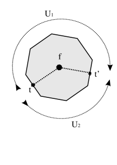
To resolve this ambiguity, we make use of the orientation of the face : this orientation gives a notion of clockwise and counterclockwise around the link. We choose the convention that denote the holonomy around the chain in the clockwise direction, starting at and ending at . (For on the boundary, or when one is considering a single -simplex, of course the orientation of need not be used to resolve this ambiguity.)
The arbitrariness in the choice of the orthonormal basis at each tetrahedron is reflected in the local gauge transformations
| (33) | |||||
| (34) | |||||
| (35) | |||||
| (36) |
where are the gauge parameters associated with the choice of basis in tetrahedra and vertices respectively.
In each tetrahedron , consider the bivector two-form
| (37) |
and its dual
| (38) |
In components, this is where
| (39) |
Now, consider a tetrahedron and a triangle in its boundary. Associate a bivector to the triangle , as follows. is defined as the surface integral of the two-form over the triangle
| (40) |
This is the geometrical bivector naturally associated to the (oriented) triangle, in the frame associated to the tetrahedron . Its dual bivector is . A single triangle belongs to (the boundary of) the several tetrahedra that are around its link. The bivectors are different, because they represent the triangle in the internal frames associated to distinct tetrahedra. But they are of course related by
| (41) |
Notice that if the tetrad is Euclidean and the triangle is in the (1,2) plane, the only non-vanishing components of are , while the only non-vanishing components of are . More in general, if the normal of the tetrahedron is , then for all the faces of the tetrahedron we have
| (42) | |||||
| (43) |
In particular, if we choose a gauge where , we have
| (44) | |||||
| (45) |
The quantities and can be taken as a discretization of the continuous gravitational fields and that define GR in the Plebanski formalism.
3.1 Constraints on
Since our aim is to promote to an independent variable, let us study the constraints it satisfies. It is immediate to see that the four bivectors associated to the four faces of a single tetrahedron satisfy the closure relation
| (46) |
Since the two-form is defined in terms of a tetrad field, it satisfies the relation (15), or, equivalently, (16,17,18). Multiplying these relations by the coordinate bivectors representing triangles, gives the following relations. For each triangle , we have
| (47) |
For each couple of adjacent triangles , we have
| (48) |
We call these two constraints the diagonal and off-diagonal simplicity constraints, respectively.
The last constraint, for and in the same four simplex sharing just a point, is a little subtler. It is
| (49) |
where is the four volume of the simplex and the sign depends on relative face orientation [21]. Of course the volume in the last formula is irrelevant. What this equation tells us is that the volume is the same when computed with different choices of pairs of faces in the same four simplex. Now, using the transformation law for the bivectors (41) one can write it with tetrads defined on tetrahedra:
| (50) |
One can show that if (31) is satisfied and the first set of constraints (46,47,48) is satisfied then (49) or, equivalently, (50) is satisfied automatically.
Let’s count the degrees of freedom for each four simplex, as a check. We start with the degrees of freedom of the bivectors, for each face. The constraint (46) imposes independent equations. The number of independent equations of the type (47) are , and finally the constraints of the type (48) contribute independent equations. The last constraint is implicitly imposed when we consider the tetrahedra to belong to the same four simplex. We are left with the degrees of freedom of the tetrad .
There is however some additional discrete degeneracy. The set of constraints (46,47,48) has two classes of solutions (see appendix B):
| (51) |
and
| (52) |
These two sectors of Plebanski theory are well known in the literature (see [5],[21]); they correspond to the fact, remarked above, that both and satisfy the same equations (46,47,48). Because of the double solution (51) and (52), these constraints do not determine uniquely.
However, we can give the off-diagonal simplicity constraints a different and slightly stronger form, which fixes this degeneracy, and which will play a role below. We can replace the off-diagonal simplicity constraints with the following requirement: that for each tetrahedron there exist a covariant vector such that (43) holds for all the faces of the tetrahedron . It is immediate to see that this implies the off-diagonal simplicity constraints, and that it is implied by the physical solution (51) of these constraints. Equivalently, we require that there is a gauge in which (45) holds. The geometry of this requirement is transparent: is the normal to the tetrahedron in four dimensions, and (43), or (45), require that the faces of the tetrahedron are all confined to the 3d hyperplane normal to .
3.2 Relation with geometry
How do we read out the geometry of the riemannian manifold, from the variables defined? First, it is easy to see that the area of a triangle is, up to a constant factor, the norm of its associated bivector:
| (53) |
Notice that the l.h.s. is independent of . This is consistent because the relation between and is an transformation, whence the norm is invariant, . This shows that the definitions chosen are consistent with a characteristic requirement of a Regge triangulation: the boundaries of the flat 4-simplices match, and in particular the area of a triangle computed from any side is the same. Of course, it follows that the same is true for the volume of each tetrahedron.
Given two triangles and in the same tetrahedron , there is a dihedral angle between the two. This angle can be obtained from the product of the normals
| (54) |
These are also invariant, hence well defined independently from the tetrahedron. The two gauge invariant quantities and characterize the geometry entirely. Notice that we can view the area as the “diagonal” part of and write .
It is important to notice that, as mentioned in the previous section, the area is also (the square root of) the norm of its associated selfdual, or, equivalently, antiselfdual bivector:
| (55) |
These equalities are assured by the simplicity constraints on . Similarly,
| (56) |
Again, these equalities follow from the simplicity constraints.
There exist a number of relations among the quantities within a single 4-simplex.555As a discussion of these relations does not seem to appear elsewhere in the literature, we have here included an appendix on them (A). Only 10 of these quantities can be independent, because the geometry of a 4-simplex is determined by 10 numbers. In particular, all angles must be given functions of the 10 areas (up to degeneracies). Explicit knowledge of the form of these functions would be quite useful in quantum gravity.
Finally, consider now a triangle . Let be the set of the tetrahedra in the link around and be the corresponding set of simplices in this link, where bounds and and so on cyclically. In general, if we parallel transport across simplices around a triangle, using , we come back rotated, because of the curvature at the triangle (the analog of a parallel transport around the tip of a pyramid in 2d.) In other words, we can always gauge transform to within a single cartesian coordinate patch, but in general there is no cartesian coordinate patch around a face. We define
| (57) |
or, equivalently
| (58) |
the product of the rotation matrices obtained turning along the link of the triangle , beginning with the tetrahedron . The rotation matrix then represents the curvature associated to the triangle , written in the -frame.
3.3 Dynamics
The last step before attacking the quantization of the model is to write the discretized action. Take the as independent variables so that . In analogy with Regge calculus we define the action to be
| (59) |
where we recall that . The first sum is over all faces in the interior of the discretization and is defined as in (58), where is any one of the tetrahedra in the link of . We impose a priori equation (41), which implies 666It follows that, for each , there is only one independent in the link. This is consistent with the action (59), where only one in each link appears. Note it follows that we are also imposing a priori (60) so that not even this one independent in the link is a priori independent of the connection degrees of freedom.
| (61) |
It follows that the first term in the action (59) is independent of the choice of tetrahedron in the link of each .
The second term in (59) is a sum over all four simplices and in each four simplex over all faces belonging to it 777This is equivalent to summing over the wedges defined by Reisenberger in [16]. Each wedge is identified by a pair .. is a lagrange multiplier living in the algebra of and varying with respect to it gives the constraint (31) on the group variables.
This action is invariant under the gauge transformations (36) and reduces to the action of GR in the limit in which the triangulation is fine. This can be seen as as follows. In the limit in which curvatures are small, , where is the plane normal to the triangle . Hence the trace gives
| (62) |
which is the GR lagrangian density.
There is also a close relation of (59) to the Regge action. To see this, let us first see how to extract the deficit angle around each face in our framework. Let denote two of the edges of the triangle . Now, as the triangle is the axis of the parallel transport around , the tangent space parallel transport map preserves each of the vectors :
| (63) |
Contracting both sides with , and inserting the resolution of unity we get
| (64) |
where . By linearity, therefore acts as identity on the subspace , forcing to belong to the subgroup fixing . Therefore is described by a single angle: this is the deficit angle around . To make this explicit, as well as to cast (59) directly into Regge-like form, let us introduce an orthonormal basis of the orthogonal complement of . The rotation is a rotation in the - plane. Therefore
| (65) |
where is the angle by which is rotated by — the deficit angle. We have also
| (66) |
Furthermore,
| (67) |
The norm of is just the area (53), which fixes the constant of proportionality here. We have
| (68) |
Thus
| (69) |
The bulk term in (59) can therefore be written
| (70) |
To lowest order in , this is precisely the bulk Regge action.
3.4 Classical equations of motion
From the form of the action (62), one can see that variation w.r.t. the tetrads will give the discrete analog of the Einstein equations. Variation with respect to the connection is more subtle. In order to proceed, let us write the action on shell w.r.t. the constraints on the group variables so that it reads where is written as in (57). The action, as we saw, is independent of the choice of the base tetrahedron in each face. Let us consider the variation with respect to . This variable appears in four terms in the sum, corresponding to the four faces of the tetrahedron . Let us choose in addition, for the sake of simplicity, the tetrahedron to be the base of these four faces. The variation () 888The variation so defined is that determined by the right invariant vector field associated to . gives
| (71) |
where is an arbitrary infinitesimal element in the algebra of . Stationarity w.r.t. these variations implies that the antisymmetric part of , seen as a four dimensional matrix, is zero. Explicitly,
| (72) |
Now, can be expanded as where is of second order in the lattice spacing 999Lattice spacing is defined with respect to a particular continuum limit. To be specific, suppose one has a metric which one wishes to approximate. Then, for each real number , one can construct a corresponding Regge geometry approximating , such that the typical lattice spacing is , as measured w.r.t. . As , approaches , and one can consider expansions in ., so that to first order we get simply,
| (73) |
which is the closure constraint. The analogous continuum equation is the Gauss constraint, given by:
| (74) |
where is the spin connection. Remembering that the tetrahedron is flat, one can choose the connection to be identically zero. Integration over the region defined by gives the closure. In order to make this relation more clear, let us consider now the case where is not the base tetrahedron for all faces. Consider then, for the face the base tetrahedron to be , where is the link around . Variation w.r.t. gives:
| (75) |
where . To first order it reads:
| (76) |
which can be seen directly as the integration of the equation (74) over the region defined by , where the spin connection is a distribution concentrated at the face in the interior of .
3.5 Topological term
Recall that in the LQG approach the action that is quantized is the Holst action [33], obtained adding to the action a topological term that doesn’t change the equations of motion
| (77) |
where is called the Immirzi parameter. The introduction of a topological term is required in order to have a theory of connections on the boundary: without it, as shown by Ashtekar, the connection variable does not survive the Legendre transform [34]. It is easy to add a similar term in the discrete theory, having no effect on the equations of motion in the continuous limit. This is
| (78) |
The reason this has no effects on the equations of motion is interesting. In a Regge geometry, the curvature associated to the face is given by the rotation . This rotation has the property of leaving the face itself invariant. Hence, it is a rotation that is generated by the dual of the face bivector itself. That is, it has the form . In the weak field limit, this gives , and therefore which vanishes because of the simplicity constraint (because is simple).
This term will play a role in the quantization.
3.6 Boundary terms
In ordinary Regge calculus boundary terms must be added to the action so that the equations of motion are the same when we vary the action with some boundary variables fixed. The other condition for boundary terms is that they add correctly. Consider a region of spacetime which is the union of two disjoint regions separated by a boundary, . The additivity condition is then that [35].
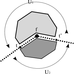
Consider for simplicity the part of the action (59) referring to a single face . Furthermore, choose two tetrahedra and appearing in the link around this face and break the link in two so that the two tetrahedra belong now to the boundary (cf. Figure 2). The action can be split to first order in the algebra as
| (79) |
where in the second term of the sum we have replaced by which, because of (41), introduces terms of the second order in the lattice spacing. are just the boundary connection variables. Here is a fixed element inserted to make the terms covariant. Thus, the boundary action can be written in general as
| (80) |
with given by
| (81) |
This gives additivity to first order in the algebra.
Let us remark on the specific case when the ’s are fixed on the boundary. In this case, in the continuum Plebanski theory, the boundary term is just where is the connection [36]. If we choose , the above discrete boundary action becomes
| (82) |
which reduces precisely to the continuum boundary action. Thus we choose when fixing the ’s on the boundary. The boundary action is not gauge-invariant, as it is not in the continuum theory.101010 One can also fix the ’s on the boundary. In this case, there is no boundary term in the continuum theory. This can effectively be achieved in the discrete theory by setting after varying the action to obtain the equations of motion (see appendix C).
Let us now write the action for a single four simplex as it will be useful to us in the next section. All the faces are on boundary and so the action is just a sum of boundary terms. Explicitly:
| (83) |
3.7 Boundary variables
Suppose the triangulation has a boundary . This boundary is a 3d manifold, triangulated by tetrahedra separated by triangles. Notice that, unlike what happens in the bulk, each boundary tetrahedron bounds just a single simplex of the triangulation; and each boundary triangle bounds just two boundary tetrahedra.
Let us identify the boundary variables, which reduce to the boundary gravitational field in the continuum limit. One boundary variable is simply , where is a boundary triangle and is a boundary tetrahedron. There are only two boundary tetrahedra around , one, , at the start of the link as determined by the orientation of , and the other, , at the end. It will turn out to be convenient to use the notation and for and . If desired, one can also associate variables with the reverse orientation of : , .
The other boundary variable is the group element giving the parallel transport across each triangle bounding and (not to be confused with the holonomy (57) defined above). Notice that (41) implies
| (84) |
Finally, of the constraints (46, 47, 48, 43, 31), only (46, 47, 48, 43) act separately at each tetrahedron, and thus impose direct restrictions on boundary data. We call (46, 47, 48, 43) the kinematical constraints. The constraint (31) on the other hand necessarily involves bulk variables; we thus call it the dynamical constraint.
The complex dual to the boundary triangulation defines a 4-valent graph with nodes (dual to the boundary tetrahedron ) and links (dual to the boundary triangle ). It is convenient to view the boundary variables as associated to the four valent graph dual to the boundary triangulation: we have group elements associated to the links of the graph and two variables associated to the two orientations of each such link. Accordingly, we change notation, and call (for links) the oriented boundary triangles and (for nodes) the boundary tetrahedra.
Since we are in a first order formalism, the space of these variables code the phase space of discretized GR. In fact, this space is precisely the same as the phase space of a Yang-Mills lattice theory, and it can be identified as the cotangent bundle of the configuration space , where is the number of links on .
This cotangent bundle has a natural symplectic structure, which defines Poisson brackets.
| (85) |
where and are, respectively, the generators and the structure constants of . Observe that the two quantities and act very nicely as the right, and respectively, left invariant vector fields on the group. Equation (84) gives the correct transformation law between the two.
However, it is important to notice a crucial detail at this point. As pointed out in [29] and in [26], because of its peculiar structure, the cotangent bundle over carries indeed two different natural symplectic structures, related to one another by what Baez and Barrett call a flip: one is obtained from the other by flipping the sign of the antiselfdual part. That is, replacing by
| (86) |
Both structures are equivalent to the lattice Yang Mills theory Poisson brackets [32], the difference is only whether we identify the electric field with or with . We call (85) the “flipped” Poisson structure (at the risk of some confusion, since Baez and Barrett call (86) the “flipped” Poisson structure. Being flipped as everything else, is a relative notion…)
Which one is the correct Poisson structure to utilize? The classical equations of motion, which is the part of the theory that is empirically supported, do not determine the symplectic structure uniquely. In the Appendix C we study the direct construction of the symplectic structure from the action. If we take the action (59) without the topological term (78), then we have the unflipped Poisson structure (86). (This is why we call it “unflipped”.) But in order to arrive at the Ashtekar formalism and LQG, we know that the topological term is needed. As shown in the appendix, the two symplectic structures written above are recovered by taking and , respectively. We discard the first choice that gives macroscopic discrete area eigenvalue and we choose the second.111111Intermediate choices may also be of interest, but they lead to a more complicated quantum theory, involving also non-simple representations. See Appendix C.
Thus, we choose the flipped symplectic structure (85) as a basis for the quantization of theory. This choice leads to a nontrivial intertwiner space, while the opposite choice leads to the Barrett-Crane trivial intertwiner space, as we shall see below.
3.8 Summary of the classical theory
Summarizing, discretized GR can be defined by the action (59) with the appropriate boundary terms (80) now defined as a function of the variables ). That is
| (87) |
Plus the diagonal and off-diagonal simplicity constraints
| (88) | |||
| (89) |
The second can be replaced by the (stronger) condition that there is an for each such that
| (90) |
equivalently, there is a gauge in which
| (91) |
The following two other constraints follow from the equations of motion
| (92) |
and
| (93) |
4 Quantization
The quantization of the theory will proceed in three steps. First, we write the Hilbert space and the operators that quantize the boundary variables and their Poisson algebra. Second, we impose the kinematical constraints (92,88,89,91). The first two of these pose no problem. The third one, namely the nondiagonal simplicity constraints (89) require a careful discussion and some technical steps. As we shall see, we cannot impose these constraints strongly; we impose them weakly, in a sense defined below. Finally, the dynamics is specified by computing an amplitude for a state in the boundary Hilbert space [37, 38]. This amplitude is constructed by building blocks, the elementary building block being a single four-simplex.
Remarkably, we will find that the physical Hilbert space that solves the constraints is naturally isomorphic to the kinematical Hilbert space of LQG. More precisely, it is isomorphic to the set of states of LQG defined on the graph formed by the dual of the boundary triangulation. Our key result will then be a transition amplitude for a state in the Hilbert space of spin networks defined on the graph corresponding to the (dual of the) boundary of a four-simplex.
4.1 Kinematical Hilbert space and operators
The boundary phase space is the same as the one of an lattice Yang-Mills theory. We quantize it in the same manner as lattice Yang-Mills theory [32]. That is, the natural quantization of the symplectic structure of the boundary variables is defined on the Hilbert space , formed by wave functions . The variables are quantized as diagonal operators. The variables and are quantized as the left invariant —respectively right invariant— vector fields on the group. These define a representation of the flipped classical Poisson algebra (3.7).
A basis in this space is given by the states
| (94) |
Here the are matrices of the representation : two of these are associated to each link; together, they form the representation matrix , defined on the Hilbert space . At each node, and , so that defines an element of the space
| (95) |
associated to each node with fixed adjacent representations . The contraction pattern of the indices between the representation matrices and the tensors is defined by .
Next, we consider the constraints.
Strictly speaking, the closure constraint (92) does not need to be imposed at this stage, since it is not an independent constraint, but it is implemented by the dynamics, as shown in the last section. But, anticipating, let us see what is its effect. It reduces to the space formed by the states invariant under . That is, it constrains the tensors to be intertwiners . That is, it constrains to belong to the subspace , which is the space of the intertwiners. The state space obtained by imposing the closure constraint is then precisely the Hilbert space of an lattice Yang-Mills theory.
The diagonal simplicity constraint (88) restricts to the spin network states where the representation associated to the links is simple. That is, it imposes .
Let us now come to the off-diagonal simplicity constraints (89), which are of central interest to us. After (92) and (88) are satisfied, only two of the three off-diagonal simplicity constraints acting on each tetrahedron are independent. These constraints form a second class system. Imposing them strongly restricts the space of intertwiners to one unique solution given by the Barrett-Crane vertex.121212 The commutator of two of these constraints is called chirality in [7]. In [7], the chirality constraint is imposed strongly on the states as well, with the result of selecting the non-degenerate geometries corresponding to the sector (51). Notice, however, that the system formed by the the chirality and the simplicity constraints is not first class either, as the chirality, in turn, does not commute with the simplicity constraints.
In order to illustrate the problems that follow from imposing second class constraints strongly, and a possible solutions to this problem, consider a simple system that describes a single particle, but using twice as many variables as needed. The phase space is the doubled phase space for one particle, i.e., , and the symplectic structure is the one given by the commutator . We set the constraints to be
| (96) |
By defining the variables and , the constraints read: . They are clearly second class since . Suppose we quantize this system on the Schrödinger Hilbert space formed by wave functions of the form . If we impose the two constraints strongly we obtain the set of two equations
| (97) |
which has no solutions. We have lost entirely the system.
There are several ways of dealing with second class systems. One possibility, which is employed for instance in the Gupta-Bleuler formalism for electromagnetism and in string theory, can be illustrated as follows in the context of the simple model above (see for instance the appendix of [39]). Define the creation and annihilation operators and . The constraints now read . Impose only one of these strongly: and call the space of states solving this . Notice that the other one holds weakly, in the sense that
| (98) |
That is, maps the physical Hilbert space into a subspace orthogonal to . Similarly, in the Gupta-Bleuler formalism the Lorentz condition (which forms a second class system with the Gauss constraint) holds in the form
| (99) |
A general strategy to deal with second class constraints is therefore to search for a decomposition of the Hilbert space of the theory (sp. for spurious) such that the constraints map . We then say that the constraints vanish weakly on . This is the strategy we employ below for the off-diagonal simplicity constraints . Since the decomposition may not be unique, we will have to select the one which is best physically motivated. We now define this space.
4.2 The physical intertwiner state space
Consider the state space obtained by imposing the diagonal simplicity constraint, namely by taking , but not the closure constraint yet. Let us restrict attention to a single tetrahedron . The constraints (89) at act on the space associated to , which is . The closure constraint will then restrict this space to the intertwiner space . We search for a subspace of where the nondiagonal constraints vanish weakly.
First, note is a subspace of the larger space
| (100) |
which can be thought of as a tensor product of carrying spaces of representations or representations, as desired. The Clebsch-Gordan decomposition for the first factor on the right-hand side above gives
| (101) |
and similarly for the other factors. By selecting the highest spin term in each factor, we obtain a subspace
| (102) |
Orthogonal projection of this subspace into then gives us the desired . This is the intertwiner space that we want to consider as a solution of the constraints. The total physical boundary space of the theory is then obtained as the span of spin-networks in with simple representations on edges and with intertwiners in the spaces at each node. Notice that the elements in are not necessarily simple in their internal representation, in any basis. Let us study the properties of the space , and the reasons of its interest.
-
(i)
First, it is easy to see that the off-diagonal simplicity constraints (89) vanish weakly , in the sense stated above. This follows from the following consideration. A generic element of can be expanded as
(103) where defines a basis in the intertwiner space. The off-diagonal simplicity constraints are odd under the exchange of and , namely under exchange of self dual and antiselfdual sectors. But the states in are symmetric in and . Hence , that is, can be considered as one possible solution of the constraint equations.
-
(ii)
Second, let us motivate the choice of this solution. Recall that the off-diagonal simplicity constraints can be expressed as the requirement that there is a direction such that (91) holds. But this is precisely the “classical” limit of the condition satisfied by the spin- representation, as observed at the end of Section 2.2. That is, promoting (91) to the quantum theory gives the requirement that there there is a gauge in which
(104) which is (27), namely the condition satisfied by the spin- component of the representation . Equivalently, (91) implies
(105) where is the scalar Casimir in the representation and is the Casimir of the subgroup that leaves invariant, in the same representation. As it is, this relation has in general no solution in , but if we order it in slightly different manner, as in (24), (reinstating for clarity)
(106) then there is always a solution, which is given by the subspace of . Therefore the off-diagonal simplicity constraints pick up precisely the space we have defined. In other words, this space satisfies a quantum constraint, which in the classical limits becomes the classical constraint (105).
Notice that if we hadn’t chosen the flipped symplectic structure, then we would have obtained , instead of , that is, the vanishing of the Casimir. Following the same procedure as above, we would have defined the space
(107) and this is precisely the one dimensional Barrett-Crane intertwiner space. That it, it is the choice of the flipped symplectic structure that allows the selection of a nontrivial intertwiner space.
-
(iii)
Third, we have the remarkable result that is isomorphic to the intertwiner space, and therefore the constrained boundary space is precisely the LQG state space associated to the graph which is dual to the boundary of the triangulation, namely the space of the spin networks on this graph. We exhibit this isomorphism in a way that simultaneously shows a new way of viewing . We will first construct a projection . The hermitian conjugate map will then be an embedding . The image of this embedding will be none other than .
The map is simple to construct. Choose an subgroup of . As explained in Section 2.2, this choice is equivalent to the choice of an isomorphism between the two factors of . A (simple) representation is in general a reducible representation of : since acts on each duality component independently, it transforms as , where is the standard spin- representation of . This decomposes into irreducibles as
(108) Thus, begin with an spin-network state , and consider the restriction to the subgroup on each edge. As is invariant, it is in particular -invariant, and thus the restriction is a sum of spin-networks. Furthermore, because is invariant, and because all possible subgroups are related to each other by conjugation, this sum of spin-networks is independent of the choice of subgroup . The above considerations tell us that this sum is just that given by the above Clebsch-Gordan decomposition for each edge. The result of the projection is then defined to be the spin-network in this sum corresponding to the highest weight spin on each edge. Thus so-defined maps simple spin-network states to spin-network states. The spin on each edge of the spin-network is mapped to spin in the spin-network. Each intertwiner is mapped to an intertwiner simply via orthogonal projection onto the subspace .
Let us now describe the conjugate embedding . This is defined as the hermitian conjugate of , using the fact that is a linear map between Hilbert spaces. Let us describe it in detail.
Let us first describe the embedding restricted to a single intertwiner space, namely the map (that we also call) from the space of the intertwiners to . Consider an intertwiner , between the four representations . Contract it with four trivalent intertwiners between the representations , the edge with spin being contracted with the edge of the corresponding trivalent intertwiner, etc. This gives us a tensor in . is not an intertwiner, because it is not invariant, but we obtain an intertwiner by projecting it in the invariant part of ). Since is compact, this projection can be implemented by acting with a group element in each representation, and integrating over .
(109) The action can be factorized into two group elements, one acting on the self dual, and other on the anti-selfdual representations. One of the two factors can be eliminated by virtue of the invariance of the trivalent intertwiners and . What remains is an integration over just one of the representations. Using the well known relation
(110) it is easy to see that we have
(111) where the coefficients are given by the evaluation of the spin network
![[Uncaptioned image]](/html/0708.1236/assets/x3.png)
.
If we piece these maps at each node, we obtain the map of the entire LQG space into the state space of the present theory. In the spin network basis we obtain
(112) Equivalently, writing explicitly the states as functions on the groups,
(113) where indices have been omitted and stand resp. for source and target of the link . This completes the definition of the projection and the corresponding embedding of the Hilbert space of LQG into the boundary Hilbert space of the model.
-
(iv)
Let us illustrate more in detail the construction in (iii) using the standard spinor notation [40]. The vectors in can be represented as totally symmetric tensors with spinor indices , where each index is in the fundamental representation of . An element in has therefore the form
(114) here primed and unprimed indices are symmetrized independently; they live in the self dual and antiself dual components of the representation. Round brackets stand for symmetrization. By choosing to no longer distinguish between primed and unprimed indices, this intertwiner between the simple representations becomes a tensor among the representations . Because of the -invariance of , the resulting tensor does not depend on the way primed and unprimed indices are identified.
Let us first construct the projection , and corresponding embedding , for individual intertwiner spaces. The projection is simply given by symmetrizing over the spinor indices associated with each link
(115) where the index is short for , and similarly for ,, and . This symmetrization projects to an intertwiner among the representations , thereby selecting the highest weight irreducible representation in the decomposition on each edge. Notice that so that the projected intertwiner transforms under transformations.
Next, we write, for , the corresponding embedding . First, the embedding is trivially obtained by reading the indices as living in self-dual and anti-self-dual representations, respectively:
(116) This is not yet a intertwiner and in order to recover an element of the invariant subspace we have to “group average” as in equation (109).
Let us now consider the projection, and corresponding embedding, for individual spins. Consider the state space for a single link – that is, the space of square integrable functions over one single copy of . This space is spanned by the representation matrices where and . Here we restrict ourselves to simple representations . For such representation matrices, the projection is defined by
(117) That is, we first restrict to a diagonal subgroup ; such a subgroup is isomorphic to . The -representation matrix then becomes a -representation matrix; from there we project to the highest irreducible, namely the representation, as before. The corresponding embedding of spins into spins is then obviously .
Putting together the embeddings for intertwiners and spins, we obtain the embedding (113) of LQG states into the boundary state space of the model.
-
(v)
Lastly, with the embedding proposed in (iii,iv) above, and in light of (53), the constraints (105) being used to solve the off-diagonal simplicity constraints simply express the condition that three-dimensional areas as determined by the SO(4) theory match three-dimensional areas as determined by LQG.
This concludes the discussion on the implementation of the constraints. The last point to discuss is the dynamics.
4.3 Dynamics
Following the strategy stated at the start of this section, consider a triangulation formed by a single 4-simplex . Denote the boundary graph by . A generic boundary state (satisfying all kinematical constraints) is a function , where , in the image . We begin by writing the transition amplitude between sharp values of the B’s. From this we deduce the amplitude in terms of the U’s, and then compute the amplitude for the quantum state . Beginning this procedure,
| (118) | |||||
so that the amplitude in the connection representation reads:
| (119) |
The integral is over a choice of element at each node. Let us define the bra
| (120) |
The quantum amplitude for a given state in the boundary Hilbert space is:
| (121) |
As satisfies all the kinematical constraints, it is of the form for some . Let us consider the specific case when is a spin-network state . The amplitude is then given explicitly by
| (122) |
as can be easily seen by using (112) and decomposing (119) in the spin-network basis. This amplitude extends by linearity to more general states .
When we have a number of transitions between different 4-simplices, we have to sum over boundary states around each, projecting each onto this state . This gives transition amplitudes for boundary spin networks with the amplitude generated by the partition function
| (123) |
Observe that the quantum dynamics defined above does not change if we add the topological term (78) incorporating . For, by changing the integration variable to in the path-integral, the above derivation goes through in exactly the same manner, and the final vertex amplitude differs at most by a constant, as determined by the Jacobian of the transformation from to (see appendix C).
The problem is whether this quantum dynamics defines a non-trivial theory with general relativity as its low energy limit. A way of systematically exploring the low-energy behavior of a background independent quantum theory has recently been developed (after a long search; see for instance [41]) in [15]. These techniques should shed some light on this problem.
5 Conclusions
We close with three observations.
(i) There is a relation of the states determined in this model to the projected spin network states studied by Livine in [42]. (A similar approach is developed by Alexandrov in [44].) The constrained states that form the physical Hilbert space of the model presented here can be constructed from (the euclidean analog of) these projected spin networks. The Euclidean analog of the projected spin networks defined in [42] are wavefunctions depending on an group element for each link, and a vector at each node. The wavefunctions are labelled by an representation for each link, an representation for each node and link based at that node, and an intertwiner at each node. The spin-networks of the present paper can be obtained from these projected spin networks by (i) setting , (ii) setting , and (iii) averaging over at each node (concretely this averaging can be done by acting on each with an element , and then averaging over the ’s independently using the Haar measure). Each of these three steps corresponds directly to solving (i) the diagonal simplicity constraints, (ii) the off-diagonal simplicity constraints, and (iii) the Gauss constraint.
(ii) Livine and Speziale have found an independent derivation of the vertex proposed here [45], based on the use of the coherent states they have introduced in [18].
(iii) The discreteness introduced by the Regge triangulation should not be confused with the quantum-mechanical discreteness. The last is realized by the fact that variables that give a physical size to a Regge cell turn out to have discrete spectrum. However, the two “discretenesses” end up to be related, because, due to the quantum discreteness, in the quantum theory the continuum limit of the Regge triangulation turns out to be substantially different that the continuum limit of, say, lattice QCD or classical Regge calculus. Intuitively, one can say that no further triangulation refinement can capture degrees of freedom below the Planck scale, since these do not exist in the theory. The ultraviolet continuum limit is trivial in the quantum theory (for a discussion of this point, see [3]). Thus, in the quantum theory the Regge triangulation receives, so to say a posteriori, the physical interpretation of a description of the fundamental discreteness of spacetime (the one, say, that makes gravitational entropy finite [46]). Numerous approaches to quantum gravity start from the assumption of a fundamental spacetime discreteness ([47]); others use spacetime discreteness as a regularization to be removed ([48]); the conventional formulation of loop quantum gravity derives the discretization of spacetime from the quantization of continuum general relativity. The derivation of loop quantum gravity given here is somewhat intermediate: it starts from a lattice discretization, and later finds out that in the quantum theory, say, the area of the triangles of the triangulation is discrete and therefore the regularization receives a physical meaning. See also [27].
In summary. We have considered the Regge discretization of general relativity. We have described it in terms of the Plebanski formulation of GR. We have quantized the theory, on the basis of a flipped Poisson structure and imposing the off-diagonal simplicity constraints weakly. This new way of imposing the simplicity constraints is weaker. This weakening of the constraints is motivated by the observation that they do not form a closed algebra, as well as by the realization that a richer boundary space is needed for a correct classical limit [14].
The theory we have obtained is characterized by the fact that its boundary state space exactly matches that of () loop quantum gravity. This can be seen as an independent derivation of the loop quantum gravity kinematics, and, in particular, of the fact that geometry is quantized. A vertex amplitude has then been derived from the discrete action, leading to a spin-foam model giving transition amplitudes for loop quantum gravity states.
We expect that the model considered here will admit a group field theory formulation [30] and that its vertex can be used to generate the dynamics of loop quantum gravity also in the absence of a fixed triangulation [3]. Whether this model is non-trivial and/or reproduces general relativity in an appropriate limit we do not know. Study of its semi-classical limit and -point functions [15] should shed light on the discussion.
————————————
Thanks to Alejandro Perez for help, criticisms and comments, to Sergei Alexandrov, Etera Livine, Daniele Oriti and Simone Speziale for useful discussions. JE gratefully acknowledges support by an NSF International Research Fellowship under grant OISE-0601844
Appendix A 4-simplex geometry as gravitational field
In the way we have defined the Regge triangulation above, the degrees of freedom of the gravitational field are captured by the geometry of each 4-simplex. Consider in each 4-simplex Cartesian coordinates such that one vertex of the 4-simplex, say the vertex 5, has coordinates , and the other four vertices have coordinates . In these coordinates, the metric will not necessarily be , but rather take a form . The full information about the geometry of the four simplex is then coded into the ten quantities . Notice indeed that the shape of a 4-simplex in is determined by 10 quantities (for instance the length of its ten sides), and therefore the ten components of are the correct number for capturing its degrees of freedom (possibly up to discrete degeneracies).
In particular, (we will often drop the argument in the rest of this appendix, since we deal here with a single 4-simplex) are (the square of) the lengths of the four edges adjacent to the 5th vertex, and are essentially the angles between these edges. (Also: is the volume of the tetrahedron , opposite to the vertex , and is the variable giving the angle between the normals to the tetrahedra and .)
Thus, the discretized variables can be taken to be the ten quantities . This is of course no surprise at all, since this is precisely a direct discretization of the variable used by Einstein to describe the gravitational field, here reinterpreted simply as a way to represent the geometry of each elementary 4-simplex.
Another way of determining the geometry of a four simplex is to give its ten areas. Let label the five tetrahedra bounding the 4-simplex. The tetrahedron 1 is the one with vertices 2,3,4,5, and so on cyclically. Let denote the triangle bounding the two tetrahedra and . The triangle has vertices , and so on cyclically. Let be the area of the triangle . Consider in particular the six areas , of the six faces adjacent to the vertex 5. A short computation, for instance using (53), shows that
| (124) |
Define the angle variables , related to the angle between the triangles and . (We can also write .) Then again:
| (125) |
The closure relation of the bivectors of a tetrahedron implies
| (126) |
and so on cyclically. The six equations (124) and the the four equations (126) express the ten areas as functions of the ten components of the metric. Inverting these equations gives the metric as a function of the areas: , and then, via (125), the angles as functions of the areas: . Therefore the full geometry of one 4-simplex is determined by the ten areas . Computing the two functions , and explicitly would be of great utility for quantum gravity.
Appendix B Existence of tetrad
In this appendix we show that the constraints (46, 47, 48), at the classical discretized level, are sufficient to imply the existence of a tetrad associated with each tetrahedron . The main point is that the ‘dynamical constraint’ (49 or 50) is not needed for the existence of . Rather, as explained in the main text, the role of (49) or (50), or its reformulation as (31), is to ensure that the geometries of the tetrahedra in a single 4-simplex fit together to form a single 4-geometry.
The triad portion of the tetrad associated with the 3-plane of the tetrahedron is uniquely determined (up to an overall sign) by the ’s of the faces of the tetrahedron. The last component of the tetrad associated with the normal to , however, is not determined by the ’s associated with . This final component is fixed only upon comparing with the tetrads at the other tetrahedra in the 4-simplex via the parallel transport maps .
Let us make all of this precise. Let denote the portion of space-time associated with one of the 4-simplices . is a 4-manifold. Equip the tangent bundle of with a background flat connection (so that we have a natural notion of parallel translation between any two points, and a natural notion of straightness).131313 Within a single 4-simplex, or any non-closed chain of 4-simplices, the choice of such a connection is a pure gauge choice. In , consider a tetrahedron with faces labeled 1,2,3, and 4. For each face, we let denote the associated bivector living in the tangent space of . These bivectors satisfy
| (127) |
What we wish to show in this appendix is that the discretized constraints (46, 47, 48) are sufficient to imply that either
| (128) |
or
| (129) |
for some tetrad . We begin with a
Lemma 1.
If is such that for , and
| (130) |
then as well. An analogous statement holds with replaced by .
Proof.
Thus, if we find a tetrad compatible with only (in the sense of (128) or (129)), then by imposing equation (130) (the closure constraint), will then automatically be compatible with the same tetrad, in the same sense. In other words, by using the closure constraint, we can ignore .
Let denote the point in the tetrahedron shared in common by faces 1,2, and 3. Let denote the three edges emanating from this point, numbered such that face 1 is between and , etc, cyclically. Then we can choose our sign conventions such that
| (132) |
Specifying a tetrad is then equivalent to specifying the three internal vectors
| (133) |
and the external unit normal to the tetrahedron. In terms of the tetrad,
| (134) |
where is the unit normal to . In terms of these variables, the condition for becomes
| (135) |
and likewise the condition becomes
| (136) |
We are now in a position to state the principal proposition and sketch its proof.
Proposition 2.
If are linearly independent and are such that
| (137) |
then exactly one of the two following cases hold.
-
1.
There exists such that
(138) or
-
2.
there exists such that
(139)
In either case, is unique up to .
Proof.
Equation (137), for the case , using proposition (3.5.35) of [40], tells us that there exists such that
| (140) | |||||
| (141) |
(). From the linear independence of the ’s, we know in particular that none of them are zero. Therefore, if we define for each
| (142) | |||||
| (143) |
then and are each two dimensional. is just the two dimensional subspace uniquely determined by the bivector , whereas each is just the subspace uniquely determined by the bivector .
Let us now look at the rest of the equations (137). For each , they tell us that and are each linearly dependent. and therefore non-trivially intersect, as do and , so that
| (144) | |||||
| (145) |
But the linear independence of the ’s tells us that none of the ’s can be the same, and none of the ’s can be the same. Thus, for ,
| (146) | |||||
| (147) |
whence
| (148) | |||||
| (149) |
Let be any non-zero vector in , etc cyclically. Likewise let be any non-zero vector in , etc cyclically. One can prove that exactly one of and is three dimensional, and the other is one dimensional. To prove this is non-trivial; we leave it as an exercise to the reader. In proving this, one uses in a key way both the assumption that the ’s are linearly independent and the fact that for each , and are orthogonal complements (which one can also show).
In the case where is linearly independent, by setting , one can solve for such that (138) holds. These are unique up to , so that is unique up to . Furthermore, one can show the fact implies that there exists no such that (139) holds.
In the case where and is linearly independent, the situations are obviously reversed. There exist no such that (138) holds, whereas there exist ’s unique up to , such that (139) holds.
Thus we have the proposition.
.
Appendix C Symplectic structure
The action is
| (150) |
In the case when one fixes the variables on the boundary, one sets identity, as then the boundary term reduces to the usual classical boundary term appropriate when fixing the variables on the boundary [36]. When one fixes the ’s (i.e., the connection) on the boundary, analogy with the classical theory suggests that there should be no boundary term. However, in a discrete theory this is not literally possible, as then no boundary variables would appear in the action at all. For the case of fixing the ’s on the boundary, we therefore suggest the following prescription. We want the terms in the boundary sum to essentially be the same as the terms in the interior sum: this will be the case if is the holonomy around the rest of the link of outside of . Of course, the problem is that this part of the holonomy around is not determined by any dynamical variables. We propose the following prescription. Whenever varying the action, keep the ’s fixed; however, whenever evaluating anything on extrema of the action, set equal to what we know it ‘should’ be: namely, the holonomy along the part of the link of outside of as determined by the BF equations of motion. The BF equations of motion dictate that all holonomies around closed loops are trivial. Thus, our prescription is, whenever evaluating an expression onshell, set . A remark is in order as to why the BF equations of motion are used. The BF equations of motion are the equations of motion coming from the unconstrained action (150). We use the unconstrained action in deriving the symplectic structure because our general philosophy is that we are quantizing GR as a BF theory constrained at the quantum level. That is, we first compute the symplectic structure and quantize everything as though it were pure BF theory. Only then, after the ‘kinematical’ quantization is complete, do we impose the simplicity constraints and obtain GR.
Let us determine the symplectic structure from the action, when we fix the ’s on the boundary. We will use a method essentially coming from that described in [49], and briefly mentioned in [2]; the method is the following. We first apply an arbitrary variation to the action without fixing any variables on the boundary; then we restrict to solutions of the equations of motion. The result will be a boundary term depending linearly on the variation. This gives us a linear map from variations (at the space of solutions) into real numbers. This linear map is then extended off-shell basically by keeping the same expression in terms of the basic variables.141414If there are constraints, this expression has ambiguities. One uses the “obvious”, simplest expression in this case. We thereby obtain a linear map from arbitrary variations of boundary data into real numbers — that is, a one-form on the space of boundary data. This is the canonical one form on the boundary phase space. The symplectic structure is then the exterior derivative .
Let us apply this procedure. Varying the action (150) gives
| (151) | |||||
Next, restrict to the case of ’s and ’s that satisfy the equations of motion. Then, when on the boundary is zero for , the entire expression above must vanish. But only the fourth term depends on for . Therefore, the other terms must vanish (on solutions) no matter what is on the boundary. Therefore, on solutions, at most the fourth term above can survive, and we have
| (152) |
Applying the equations of motion to , we finally set , giving us
| (153) |
Extending to arbitrary variations of the boundary data, keeping the same expression in terms of the basic variables, we obtain the canonical one-form
| (154) |
We next claim that is an element of . To show this, let denote a one-parameter path in such that is the tangent to the path at . Then
| (155) |
The argument in brackets is the identity at , so that one has the action of a tangent vector at the identity on the matrix elements of the group. Thus one has an element of the Lie algebra.
Introduce a basis of , orthonormal with respect to the trace — i.e. such that . Denote the components of a Lie algebra element with respect to this basis just by adding a superscript or subscript. (154) can then be written
| (156) |
Define
| (157) |
so that is a one-form on the copy of parametrized by . We can then write the canonical one form as
| (158) |
For each face , and each basis element , let denote the corresponding right invariant vector field on the associated copy of . We then have
| (159) |
Thus the form the basis of right invariant one-forms dual to the basis of right invariant vector fields. These right invariant one forms have been well studied, for example, by Cartan [50]. They satisfy
| (160) |
where are the structure constants of the Lie algebra. Using this identity to compute the symplectic structure from , we obtain
| (161) |
From this, one can read off the Poisson brackets. As there are no terms, the ’s commute. The first term above gives the Poisson bracket between the ’s and the ’s, and the second gives the Poisson brackets among the ’s. Explicitly,
| (162) | |||||
| (163) | |||||
| (164) |
The second two equations can be summarized by stating that the action generated by on is that of the right invariant vector field field determined by . The above Poisson brackets can also be more explicitly written in terms of matrix elements
| (165) | |||||
| (166) | |||||
| (167) |
If we define , this becomes (3.7).
Thus we obtain the symplectic structure from the action when we fix the ’s on the boundary. The case of fixing the ’s on the boundary is not as well-understood. Application of the above prescription to this case seems to lead to a non--gauge-invariant symplectic structure in which all the ’s commute. For the present, we simply do not address this problem, and take the symplectic structure to be the one determined with ’s fixed.
So far we have seen that the action we have considered gives the unflipped Poisson structure.
Recall, however, that in the LQG approach the action that is quantized is the GR one with a topological term that doesn’t change the equations of motion:
| (168) |
where is the so called Immirzi parameter. Recall that the introduction of this topological term is required in order to have a theory of connections on the boundary: without it, as shown by Ashtekar, the connection variable does not survive the Legendre transform [34]. Let us therefore consider the discretization of the modified BF action:
| (169) |
and follow the lines presented in this paper. Define then ; the symplectic structure is then such that, for each face, the are identified with the generators of . The constraints imply, in terms of these new variables:
| (170) |
Note that for and one recovers the same constraint being used before, whence, in these two limits, the diagonal simplicity constraints again imply simplicity of the representations of the edges (). (Thanks to Alejandro Perez for pointing this out.) Furthermore, as mentioned in §4.3, neither does the dynamics change with the introduction of the -term in the action. What is different, then, with the introduction of the term, when or ? In the case, the symplectic structure in terms of is different — it is the flipped symplectic structure. Is there an independent reason to prefer over ? Yes: the latter is unphysical, because it leads to a macroscopic area spectrum in the boundary theory. Thus, when we look at things more carefully, we do in fact see that the flipped symplectic structure is a consistent choice. And with this flipped symplectic structure, as noted in the main text, the off-diagonal simplicity constraints, in the form (105), lead precisely to the model presented in this paper.
As a side remark, consider the case . In this case, one obtains the more standard symplectic structure (86). As noted in §4.2, this symplectic structure, along with the constraint (105), imposed as discussed above, leads to the Barrett-Crane model. Thus the case, which we argue against, can be viewed as yielding the Barrett-Crane model.
References
-
[1]
C Rovelli, L Smolin, “Knot theory and quantum gravity”
Phys. Rev. Lett. 61 (1988) 1155-1158.
C Rovelli, L Smolin, “Loop space representation for quantum general relativity”, Nucl. Phys. B331 (1990) 80-152.
A Ashtekar, C Rovelli, L Smolin, “Weaving a classical geometry with quantum threads”, Phys. Rev. Lett. 69, 237 (1992).
C Rovelli, L Smolin, “Discreteness of Area and Volume in Quantum Gravity”, Nucl. Phys. B442 (1995) 593-619; Erratum: Nucl. Phys. B456, 734 (1995).
A Ashtekar, J Lewandowski, “Quantum Theory of Geometry I: Area Operators” Class. Quant. Grav. 14 (1997) A55-A82.
A Ashtekar, J Lewandowski, “Quantum Theory of Geometry II : Volume Operators”, Adv. Th. Math. Phys. 1 (1997) 388-429. -
[2]
A Ashtekar, J Lewandowski, “Background independent quantum
gravity: A status report”, Class. Quant. Grav. 21 (2004)
R53-R152.
A Ashtekar, “An introduction to loop quantum gravity through cosmology”, arXiv:gr-qc/0702030.
L Smolin, “An invitation to loop quantum gravity”, arXiv:hep-th/0408048.
T Thiemann, Introduction to Modern Canonical Quantum General Relativity (CUP, to appear). - [3] C Rovelli, Quantum Gravity (Cambridge University Press, Cambridge, 2004).
-
[4]
T Thiemann “Quantum spin dynamics (QSD)” Class. Quant.
Grav. 15 (1998) 893-873.
T Thiemann, Quantum spin dynamics VIII. The Master Constraint Class. Quant. Grav. 23 (2006) 2249-2266. -
[5]
MP Reisenberger, C Rovelli,
“ ‘Sum over surfaces’ form of loop quantum gravity”,
Phys. Rev. D56, 3490 (1997) [arXiv:gr-qc/9612035].
JC Baez, “Spin foam models”, Class. Quant. Grav. 15 (1998) 1827-1858.
MP Reisenberger, C Rovelli, “Spin foams as Feynman diagrams”, in Florence 2001, A relativistic spacetime odyssey ed. I Ciufolini, D Dominici, L Lusanna (World Scientific, Singapore, 2003) pp 431-448, [gr-qc/0002083].
JC Baez, “An introduction to spin foam models of BF theory and quantum gravity”, Lect. Notes Phys. 543 (2000) 25-94.
MP Reisenberger, C Rovelli, “Spacetime as a Feynman diagram: The connection formulation”, Class. Quant. Grav. 18 (2001) 121-140. - [6] MP Reisenberger, “A lattice worldsheet sum for 4-d Euclidean general relativity”, arXiv:gr-qc/9711052.
- [7] JW Barrett, L Crane, “Relativistic spin networks and quantum gravity”, J. Math. Phys. 39 (1998) 3296-3302.
-
[8]
R DePietri, L Freidel, K Krasnov, C Rovelli “Barrett-Crane
model from a Boulatov-Ooguri field theory over a homogeneous space”,
Nucl. Phys. B574 (2000) 785-806.
A Perez, C Rovelli, “A spinfoam model without bubble divergences”, Nucl. Phys. B599 (2001) 255-282.
D Oriti, RM Williams, “Gluing 4-simplices: a derivation of the Barrett-Crane spinfoam model for Euclidean quantum gravity”, Phys. Rev. D63(2001) 024022. -
[9]
D Oriti, “Spacetime geometry from algebra: spin foam models for
non-perturbative quantum gravity”, Rept. Prog. Phys.
64 (2001) 1489-1544.
A Perez, “Spin Foam Models for Quantum Gravity”, Class. Quant. Grav. 20 (2003) R43. - [10] G Ponzano, T Regge, “Semiclassical limit of Racah coefficients” in Spectroscopy and Group Theoretical Methods in Physics ed. F. Bloch (North-Holland, Amsterdam 1968).
- [11] C Rovelli, “Basis of the Ponzano-Regge-Turaev-Viro-Ooguri quantum gravity model is the loop representation basis”, Phys. Rev. D48 (1993) 2702.
- [12] K Noui, A Perez “Three dimensional loop quantum gravity: physical scalar product and spin foam models”, Class. Quant. Grav. 22 (2005) 1739-1762
-
[13]
A Perez, “Finiteness of a spinfoam model for
euclidean GR”, Nucl. Phys. B599 (2001) 427-434.
L Crane, A Perez, C Rovelli, “Finiteness in spinfoam quantum gravity”, Phys. Rev. Lett. 87 (2001) 181301.
L Crane, A Perez, C Rovelli, “A finiteness proof for the Lorentzian state sum spinfoam model for quantum general relativity”, [arXiv:gr-qc/0104057]. - [14] E Alesci C Rovelli, “The full LQG graviton propagator: I. Difficulties with the Barrett-Crane vertex”, arXiv:0708.0883.
-
[15]
C Rovelli, “Graviton propagator from
background–independent quantum gravity”,
Phys. Rev. Lett. 97 (2006) 151301
[arXiv:gr-qc/0508124].
L Modesto, C Rovelli: “Particle scattering in loop quantum gravity”, Phys. Rev. Lett. 95 (2005) 191301. E Bianchi, L Modesto, C Rovelli, S Speziale “Graviton propagator in loop quantum gravity” Class. Quant. Grav. 23 (2006) 6989-7028.
S Speziale, “Towards the graviton from spinfoams: the 3d toy model”, JHEP 0605, 039 (2006) [arXiv:gr-qc/0512102].
E Livine, S Speziale, J Willis, “Towards the graviton from spinfoams: higher order corrections in the 3d toy model”, Phys. Rev. D 75, 024038 (2007) [arXiv:gr-qc/0605123].
ER Livine, S Speziale, “Group integral techniques for the spinfoam graviton propagator”, JHEP 0611, 092 (2006) [arXiv:gr-qc/0608131].
B Dittrich, L Freidel, S Speziale, “Linearized dynamics from the 4-simplex Regge action”, arXiv:0707.4513 [gr-qc]. - [16] MP Reisenberger, “A left-handed simplicial action for euclidean general relativity”, Class. Quant. Grav. 14, 1753 (1997) [arXiv:gr-qc/9609002].
-
[17]
S Alexandrov
“Choice of connection in Loop Quantum Gravity” Phys Rev D65
(2002) 024011.
S Alexandrov, E Livine, “SU(2) Loop Quantum Gravity seen from Covariant Theory”; Phys. Rev. D67 (2003) 044009.
E Buffenoir, M Henneaux, K Noui, Ph Roche, “Hamiltonian Analysis of Plebanski Theory”, Class. Quant. Grav. 21 (2004) 5203-5220. - [18] ER Livine, S Speziale, “A new spinfoam vertex for quantum gravity”, arXiv:0705.0674
- [19] PAM Dirac, Lectures on Quantum Mechanics (Yeshiva University, New York 1964)
- [20] J Engle, R Pereira, C Rovelli, “The loop-quantum-gravity vertex-amplitude”, arXiv:0705.2388 [gr-qc].
-
[21]
A Perez:
“Spin foam quantization of SO(4) Plebanski’s action”,
Adv. Theor. Math. Phys. 5 (2002) 947
[Erratum-ibid. 6 (2003) 593].
L Freidel, K Krasnov, “Spin Foam Models and the Classical Action Principle”, Adv. Theor. Math. Phys. 2 (1999) 1183-1247.
R De Pietri, L Freidel, “so(4) Plebanski Action and Relativistic Spin Foam Model”, Class. Quant. Grav. 16, 2187 (1999) [arXiv:gr-qc/9804071].
MP Reisenberger, “Classical Euclidean general relativity from *left-handed area = right-handed area*”, arXiv:gr-qc/9804061. - [22] G Immirzi, “Quantum gravity and Regge calculus”, Nucl. Phys. Proc. Suppl. 57 (1997) 65 [arXiv:gr-qc/9701052].
- [23] T Regge, “General Relativity Without Coordinates”, Nuovo Cimento 19:558-571, (1961)
- [24] M Rocek, RM Williams, “Quantum Regge Calculus”, Phys. Lett. B 104 (1981) 31.
- [25] RM Williams, “Introduction to Regge calculus”, lecture notes at the First Quantum Geometry and Quantum Gravity School, Zakopane, Poland March 23 - April 3, 2007, to appear.
- [26] JC Baez and JW Barrett, “ The Quantum tetrahedron in three-dimensions and four-dimensions”, Adv. Theor. Math. Phys. 3:815-850, (1999).
- [27] JA Zapata, “Loop quantization from a lattice gauge theory perspective”, Class. Quant. Grav. 21 (2004) L115 [arXiv:gr-qc/0401109].
- [28] NDH Dass, M Mathur, “On loop states in loop quantum gravity,” Class. Quant. Grav. 24 (2007) 2179 [arXiv:gr-qc/0611156].
- [29] M Montesinos, “Alternative symplectic structures for SO(3,1) and SO(4) four-dimensional BF theories”, Class. Quant. Grav. 23 (2006) 2267, [arXiv:gr-qc/0603076].
-
[30]
L Freidel, “Group Field Theory: an overview”,
Int. Journ. Theor. Phys. 44 (2005) 1769-1783.
D Oriti, “The group field theory approach to quantum gravity”, arXiv:gr-qc/0607032. - [31] MP Reisenberger, “On relativistic spin network vertices”, J. Math. Phys. 40 (1999) 2046 [arXiv:gr-qc/9809067].
- [32] M Creutz, “Gauge Fixing, the Transfer Matrix, and Confinement on a Lattice”,, Phys. Rev. D15, 1128, (1977).
- [33] S Holst “Barbero’s Hamiltonian derived from a generalized Hilbert-Palatini action” Phys. Rev. D53 (1996) 5966-5969.
- [34] A Ashtekar, Lectures on Non-perturbative Canonical Gravity (World Scientific, Singapore, 1991).
- [35] JB Hartle and R Sorkin, “Boundary Terms In The Action For The Regge Calculus”, Gen. Rel. Grav. 13:541-549,(1981).
- [36] D Oriti, “Boundary terms in the Barrett-Crane spin foam model and consistent gluing”, Phys. Lett. B532:363-372 , (2002).
- [37] R Oeckl, “A ‘General boundary’ formulation for quantum mechanics and quantum gravity”, Phys. Lett. B575:318-324, (2003).
- [38] C Rovelli, “The Projector on physical states in loop quantum gravity”, Phys. Rev. D59:104015, (1999).
- [39] RS Tate, “ An Algebraic approach to the quantization of constrained systems: Finite dimensional examples”, Ph.D. Thesis, e-Print: gr-qc/9304043.
- [40] Penrose R and Rindler W 1984 Spinors and Spacetime vol. 1 (Cambridge: Cambridge UP).
- [41] J Iwasaki, C Rovelli, “Gravitons as embroidery on the weave,” Int. J. Mod. Phys. D 1 (1993) 533.
- [42] E Livine, “Projected spin networks for Lorentz connection: Linking spin foams and loop gravity”, Class. Quant. Grav. 19 :5525-5542, (2002).
- [43] RE Livine, D Oriti, “Barrett-Crane spin foam model from generalized BF type action for gravity”, Phys. Rev. D65:044025, (2002).
- [44] S Alexandrov, “Spin foam model from canonical quantization”, arXiv:0705.3892 [gr-qc].
- [45] ER Livine, S Speziale, “A new spinfoam vertex for quantum gravity”, [arXiv:0705.0674, gr-qc].
- [46] C Rovelli, “Loop quantum gravity and black hole physics”, Helv. Phys. Acta 69 (1996) 582 [arXiv:gr-qc/9608032].
-
[47]
M Campiglia, C Di Bartolo, R Gambini, J Pullin,
“Uniform discretizations: A new approach for the quantization of totally
constrained systems”, Phys. Rev. D74: 124012, (2006).
R Gambini, J Pullin, “Canonical quantization of general relativity in discrete space-times” Phys. Rev. Lett., 90 021301 (2003).
K Giesel, T Thiemann, “Algebraic quantum gravity (AQG). I: Conceptual setup”, Class. Quant. Grav. 24 2465 (2007).
R Sorkin, “Causal Sets: Discrete Gravity”, in Proceedings of the Valdivia Summer School, A Gomberoff, D Marolf, eds. (Plenum, New York, 2005). - [48] J Ambjorn, J Jurkiewicz, R Loll, “Quantum Gravity, or The Art of Building Spacetime”, in Approaches to Quantum Gravity, D Oriti ed. (Cambridge University Press, to appear), arXiv:hep-th/0604212v1.
-
[49]
A Ashtekar, L Bombelli and O Reula “Covariant phase space of
asymptotically flat gravitational fields”, in Mechanics,
Analysis and Geometry: 200 Years after Lagrange, Ed. by M
Francaviglia and D Holm (North Holland, Amsterdam 1991).
A Ashtekar, L Bombelli, and R Koul “Phase space formulation of General Relativity without 3+1 splitting”, in The Physics of Phase Space, Ed. by Y S Kim and W W Zachary (Springer-Verlag, Berlin, 1987). - [50] Y Choquet-Bruhat, C DeWitt-Morette, M Dillard-Bleick, Analysis, Manifolds, and Physics (North-Holland, Amsterdam 1982).