TAUP-2861/07 UTTG-04-07
Localized Backreacted Flavor Branes
in Holographic QCD
Benjamin A. Burrington, Vadim S. Kaplunovsky,
Jacob Sonnenschein
†School of Physics and Astronomy,
The Raymond and Beverly Sackler Faculty of Exact Sciences,
Tel Aviv University, Ramat Aviv, 69978, Israel.
∗University of Texas at Austin
Theory Group, Physics Department,
1 University Station, C1608
Austin, TX 78712 1608, USA
We investigate the perturbative (in ) backreaction of localized D8 branes in D4-D8 systems including in particular the Sakai Sugimoto model. We write down the explicit expressions of the backreacted metric, dilaton and RR form. We find that the backreaction remains small up to a radial value of , and that the background functions are smooth except at the D8 sources. In this perturbative window, the original embedding remains a solution to the equations of motion. Furthermore, the fluctuations around the original embedding, describing scalar mesons, do not become tachyonic due to the backreaction in the perturbative regime. This is is due to a cancelation between the DBI and CS parts of the D8 brane action in the perturbed background.
1 Introduction
By now, AdS/CFT has become a standard tool in theoretical physics for the study of gauge theories at strong coupling. In many “stringy” models of gauge dynamics fundamental matter is included by embedding a set of “flavor branes” in addition to the “glue/color branes.” In such a setup, the strings connecting only to the “glue branes” are in the adjoint of the group, giving gauge particles (multiplets), and those connecting only to the “flavor branes” are in the adjoint of , giving the mesons (meson multiplets), and those connected to both the “flavor” and “glue” branes are in the fundamental representation of both the and groups, giving the quarks (matter/quark multiplets). Anti-quarks are obviously depicted by similar strings with the opposite orientation.
In principle for large and large one could go to a combined near horizon limit, translate the branes into fluxes 111bearing in mind that one must keep the open string spectrum associated with the flavor branes, even though they are producing macroscopic flux. Such a case is a full backreaction, but not a decoupling limit. Recall that global symmetries of the field theory translate into gauge symmetries in the gravity: gauging a large flavor group using supergravity alone is unfeasible. and derive the gravity background that is a holographic dual of a gauge system with gluons and quarks ( and, if the model is supersymmetric, their supersymmetric partners). However, in practice such models are being constructed using the probe approximation. In this approximation one uses a gravity background built from the near horizon limit of a large glue branes and adds to it a set of flavor probe branes. The basic assumption of the probe approximation is that for the case of the backreaction of the probes on the background can be neglected. The flavor physics is then extracted by analyzing the effective action that describes the flavor branes in the glue background, namely the DBI action plus the CS action. This practice was introduced in [1] in the context of the model, for a confining background in [2] and subsequently in a large variety of other models[3],[4], [5]. Exceptions to this are certain fully backreacted non critical models like [6],[7],[8], and [9].
A landmark holographic model of chiral symmetry and chiral symmetry breaking is the model of Sakai and Sugimoto[10]. This model is based on the incorporation of a stack of D8 and anti- D8 flavor branes into the background of near extremal branes[11]. In the latter background one compactifies one of the world volume coordinates of the D4 branes on a circle of radius . For energies the background describes a four dimensional system with gluon degrees of freedom plus contaminating Kaluza Klein modes. The profile of the flavor branes determined by the DBI action is that of a U shape. This provides a simple geometrical picture of chiral symmetry breaking, namely, for large radial direction (see figure 2), which corresponds to the UV limit of the gauge theory, the stack of the D8 branes and of the anti-D8 branes are separated and hence there is a symmetry, and in the IR limit the two stacks merge one into the other and thus only the diagonal survives as a symmetry. A variety of physical properties of meson and baryon physics has been extracted from the model. These include the massive meson spectrum, the massless Goldstone pions[10], certain decay rates [12] as well as the thermal behavior of hadrons [13],[14].
The validity of the model [10], is the same as all other probe models: . To contact to real hadron physics, one obviously is interested in the case where the number of flavors is similar to that of the colors and both are not large. To get down to small one will have to invoke a full string theory rather than a effective gravity model. However, increasing the ratio of can still be done in the context of an effective field theory, provided we go beyond the probe approximation and incorporate the backreaction of the flavor branes on the gravity background. This may enable us to determine the flavor dependence of certain physical properties of the gauge theory which we expect to be dependent, for example the beta function, or the ratio of viscosity to entropy density of the quark-gluon fluid [15].222In [16], the leading order correction in of this property was determined in the context of a model with D7 branes in near extremal background. However, in this model it was shown that the zero mode, which is equivalent to smearing, is all that is necessary to this level in .
Similar studies for localized backreactions in D3-D7 systems include [17, 18, 19, 20, 21]. In [17], very general framework for studying type IIB supergravity with metric/five form and holomorphic dilaton/axion. The work of [18, 19, 20] studied when the D7 branes are located at singular points in manifolds, and [21] studied the form of the solution to the equations following from the D3-D7 system and effects on other probe branes in such backgrounds. All these studies worked using the supergravity alone, while here we will derive delta function source terms from an action of the form
| (1.1) |
We will use this action to determine how to source the bulk fields. Although we obtain the full equations of motion from this, we will study their solutions in a perturbative limit. Therefore, while we are going beyond the probe approximation, we are still confined to the regime for the simple reason that we want the series in powers of to converge quickly.
In fact there is an even more important motivation to explore the model of [10] beyond the probe approximation, and that is the issue of the stability of the model. One may wonder whether the model is stable only in the probe approximation and that the backreaction of the probe branes on the background does not destabilize the setup. A simplified picture of the model is that of the circle of the compactified direction with the two endpoints of the stacks of probe branes and anti branes which can be represented as a charge located at one point on the circle and charge located at the antipodal point. In this simplified “electrostatic” setup if one of the charges gets a slight perturbation in one direction it will be attracted to the opposite charge and will not be driven back to its original location. Moreover, the antipodal setup described in [10] has been generalized to a family of setups where the separation distance between the brane and anti-brane is taken to be . For these cases the “electrostatic instability” is even more severe. The question is therefore whether this naive intuition is justified and the backreaction of the probe branes indeed destabilizes the model. On the other hand there is a naive argument why the perturbative backreacted system should be stable and non tachyonic. Since the gauge holographic dual of the model before purturbing it has a spectrum with a mass gap ( apart from the pions), a small a small perturbation cannot bridge the gap and produce tachyonic modes[22].
Further, one may wonder what happens to the the dilaton tadpole condition, given that this is a D8 on a circle, and both branes and anti branes source the dilaton in the same way. Hence, for these codimension one flavor branes one anticipates that the dilaton will have a cusp behavior at the location of the probe branes as well as a cusp (and not an anti-cusp) at the anti-brane. It seems naively that there is no way to sew together these two cusps.
Thus the goal of this paper is to compute the leading order backreacted background, and address the stability, and the dilaton tadpole. To do so, we write down the full action of the system (of the form in (1.1)) which is composed of the action of massive type supergravity and the nine dimensional DBI +CS actions associated with the the flavor branes. At this point one often invokes a smearing of the flavor branes along their transverse direction [23, 24, 25] which renders the combined action into a ten dimensional one. This approach simplifies the analysis by turning the equations of motion (EOMs) into ordinary differential equations (ODEs) of some radial variable. However, we expect that certain physical questions may not be answered using this procedure, for example the stability discussed above. Thus we avoid using the smearing technique and we keep the flavor branes as localized objects. This yields delta function source terms for the equations of motion of the graviton, dilaton and the RR field strength form associated with the D8 branes. The complexity of these equations is increased, relative to the smearing technique, because the EOMs are now partial differential equations (PDEs); the relevant functions must depend on the coordinate(s) transverse to the flavor brane. 333For this added complication, though, we simplify the equations by using a perturbative approach. In some sense, this is complimentary to smearing: one smears the branes to obtain non-linear ODEs to solve; we instead perturb the equations to obtain linear PDEs.
We solve these equations perturbatively to the leading order in . We take 3 cases for the background to help address the questions in stages, and gain intuition for how the solutions should behave.
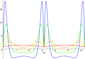
We first solve for the simplified system of a decompacitfied transverse coordinate of the D8 branes, which has been studied in its own right in [26], [27](see figure 1 (a)). For this case we were able to find exact solutions of the partial differential equations. To our surprise we have found that whereas the solutions for the perturbations of some background fields behave, as we have expected, with a cusp at the location of the probe branes (a “” shape), for other the behavior is of an inverted cusp dressed with a double hump structure (an “m”, see figure 3). We explore the ranges where we expect the supergravity to be a good description and find that , and that the perturbative results are good up to . Further, from this study, it becomes plausible that compactifying the direction is possible, as the functions die off at large .
Next, we address the compactified (but extremal) case both to view the effects of compactification, but also as a rough approximation of the “cigar” case at large (see figure 1 (b)). We first treat this case where we sum over the images of the uncomactified case, and then as a Fourier decomposition. From this we see that there is no issue with the dilaton tadpole constraint: the two cusps meets smoothly. We find that the decompactified limit emerges at large . Both methods are applied because, although both series always converge, one series converges very quickly at large , while the other converges quickly at small .
Finally we analyze the system of the near extremal D4 branes. We find that in this case the perturbation theory is good for which is generically stronger than the supergravity regime. Further, we find that the supergravity description is valid near , with the additional constraint . This translates into the requirement that where is the string tension, is the typical glueball mass, and is the ’t Hooft coupling. For large values of the radial direction the solution is obviously like that of the extremal compactified case. We use a Fourier decomposition to show that a finite expansion around the tip of the cigar is possible, and then implement this expansion for the first few terms.

Once we have established the perturbative solutions, we proceed to analyze the stability of the system. We first show that the solution of the embedding of the flavor brane at the probe level persists also in the leading order backreaction. We further show that the fluctuations of the embedding, which correspond to scalar mesons in the dual gauge theory, are non tachyonic. Hence we shown that the system is stable at least for an action that is quadratic in the fluctuations. This is due to a cancelation between the electrostatic repulsion (CS action) and the gravitational attraction (DBI action). Hence, the above analogy with an electrostatic problem is not quite justified: the electric repulsion is canceled by a gravitational attraction. The only other force is that of the tension of the brane, which is restorative. The corrections to this force, while interesting, cannot change the qualitative feature of stability while the perturbative analysis is valid (however, the effects of the non-perturbative backreaction is still an open question).
The paper is organized as follows. In the next section (2) we briefly review the general setup of the problem, namely, the Sakai Sugimoto [10] model and the massive type supergravity action [28, 29]. In section 3 we write the supergravity EOMs that incorporate the backreaction of the probe branes. We then introduce an ansatz for the metric which we substitute into the equations. The perturbative parameter is defined, and these equations are expanded. The gauge invariance, in the form of small coordinate transformations, of the system is discussed. In section 4 we present the solutions of the backreacted EOM. We start with the solutions for the uncompactified case, and then by summing over images the solutions for the compactified extremal case is constructed. We also use Fourier analysis to study this case. This enables us to determine the UV behavior of the near extremal case because the geometries are identical at large radius. The third step is to write down the solutions for the near extremal case in the region close to the horizon. In the following section we analyze the stability of the system. We first show that the solution of the EOMs that follow from the backreacted DBI+CS action are the same as those of the unperturbed solution. Finally we shown that the spectrum of fluctuations around this embedding is tachyon free and hence we conclude that to the leading order in the system is stable.
2 Brief review of the general setup
Before we start the analysis of the backreaction of the flavor branes, we briefly review the two main ingredients of the general setup of the problem, namely, the Sakai Sugimoto model and the action of the massive type supergravity. The reader familiar with these topics should skip to the next section.
2.1 Sakai-Sugimoto (SS) model
Constructing holographic models duals of gauge dynamics that admits confinement is by now a relatively easy task. Incorporating flavor chiral symmetry, on the other hand, turns out to be more complicated. A prototype model that includes both phenomena is the Sakai-Sugimoto model [10]. It is a model of a holographic dual for a dimensional gauge theory with a continuous flavor chiral symmetry which is spontaneously broken. It is based on the incorporation of D8-branes and anti-D8-branes into Witten’s model [11]. The latter describes the near horizon limit of D4-branes, compactified on a circle of radius () with anti-periodic boundary conditions for the fermions. The D8-branes are placed at and the anti-D8-branes at . The gauge theory dual of this SUGRA setup is a dimensional maximally supersymmetric gauge theory, compactified on a circle with anti-periodic boundary conditions for the adjoint fermions, and coupled to left-handed fermions in the fundamental representation of localized at , and to right-handed fermions in the fundamental representation localized at .
The basic assumption of the model is that in the limit of one can ignore the back-reaction of the D8 branes and anti-D8 branes. As mentioned above the goal of the present work is to examine in details the back-reaction of the D8 and anti-D8 on the background. With the probe assumption the closed type IIA string background is given by :
| (2.1) | ||||
where is the time direction and () are the uncompactified world-volume coordinates of the D4 branes, is a compactified direction of the D4-brane world-volume which is transverse to the probe D8 branes, is the metric of a unit four-sphere and is its volume form, and is related to the dimensional gauge coupling by . The submanifold spanned by and has the topology of a cigar with , and requiring that this has a non-singular geometry gives a relation between and ,
| (2.2) |
The parameters of this gauge theory, the five-dimensional gauge coupling , the low-energy four-dimensional gauge coupling , the glueball mass scale , and the string tension are determined from the background (2.1) in the following form :
| (2.4) |
where , is the typical scale of the glueball masses computed from the spectrum of excitations around (2.1), and is the confining string tension in this model (given by the tension of a fundamental string stretched at where its energy is minimized). The gravity approximation is valid whenever , otherwise the curvature at becomes large. Note that as usual in gravity approximations of confining gauge theories, the string tension is much larger than the glueball mass scale in this limit. At very large values of the dilaton becomes large, but this happens at values which are of order (in the large limit with fixed ), so this will play no role in the large limit that we will be interested in. The Wilson line of this gauge theory (before putting in the D8-branes) admits an area law behavior [30], as can be easily seen using the conditions for confinement of [31].
The gauge theory dual to the SUGRA background (2.1) is in fact not four dimensional even at energies lower than the Kaluza-Klein scale since the masses of the glueballs are also , namely, there is no real separation between the confined four-dimensional fields and the higher Kaluza-Klein modes on the circle. As discussed in [11], in the opposite limit of , the theory approaches the dimensional pure Yang-Mills theory at energies small compared to , since in this limit the scale of the mass gap is exponentially small compared to .
The probe flavor D8-branes span the coordinates , and trace a curve in the -plane. Near the boundary at we want to have D8-branes localized at and anti-D8-branes (or D8-branes with an opposite orientation) localized at . Naively one might think that the D8-branes and anti-D8-branes would go into the interior of the space and stay disconnected; however, these 8-branes do not have anywhere to end in the background (2.1), so the form of must be such that the D8-branes smoothly connect to the anti-D8-branes (namely, must go to infinity at and at , and must vanish at some minimal coordinate ). Such a configuration spontaneously breaks the chiral symmetry from the symmetry group which is visible at large , , to the diagonal symmetry. Thus, in this configuration the topology forces a breaking of the chiral symmetry.
To determine the profile of flavor probe branes, one has to solve the equations of motion of that follow from the DBI + CS action that describes the probe branes. It is easy to check that the CS term in the D8-brane action does not affect the solution of the equations of motion. More precisely, the equation of motion of the gauge field has a classical solution of a vanishing gauge field, since the CS term includes terms of the form and . So, we are left only with the DBI action. The induced metric on the D8-branes is
| (2.6) | |||||
where . Substituting the determinant of the induced metric and the dilaton into the DBI action, we obtain (ignoring the factor of which multiplies all the D8-brane actions that we will write) :
| (2.7) |
where is the induced metric (2.6) and includes the outcome of the integration over all the coordinates apart from . The simplest way to solve the equation of motion is by using the Hamiltonian of the action (2.7), which is conserved (independent of ) :
| (2.8) |
where on the right-hand side of the equation we assumed that there is a point where the profile of the brane has a minimum, 444This type of analysis was done previously for Wilson line configurations. See, for instance, [30].. We need to find the solution in which as goes to infinity, goes to the values ; this implies
| (2.9) |
with given (as a function of ) by (2.8) (note that is a double-valued function of in these configurations, leading to the factor of two in (2.9)). The form of this profile of the D8 brane is drawn in figure 2(a). Plugging in the value of from (2.8) we find
| (2.11) | |||||
where . Small values of correspond to large values of . In this limit we have leading to . For general values of the dependence of on is more complicated.
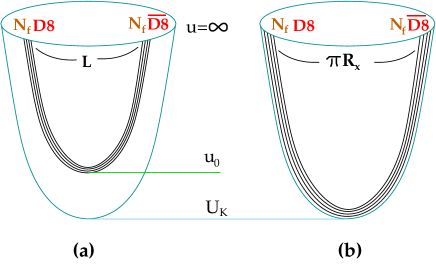
There is a simple special case of the above solutions, which occurs when , namely the D8-branes and anti-D8-branes lie at antipodal points of the circle. In this case the solution for the branes is simply and , with the two branches meeting smoothly at the minimal value to join the D8-branes and the anti-D8-branes together. This type of antipodal solution is drawn in figure 2(b). It was shown in [10] that this classical configuration is stable, by analyzing small fluctuations around this configuration and checking that the energy density associated with them is non-negative.
In general for , there is a family of smooth configurations characterized by or by the minimal value of , . This class of solution is shown in 2(a)
The Sakai-Sugimoto model has 3 dimensionful parameters : , and , and gravity is reliable whenever . The physics depends on the two dimensionless ratios of these two parameters; In the gravity limit the mass of the (low-spin) mesons is related to [13] while the mass of the (low-spin) glueballs is related to . As discussed above, in the limit this theory approaches (large ) QCD at low energies. This remains true also after adding the flavors, at least when is of order .
2.2 Massive type IIA and 8 branes
One expects dimensional objects to naturally couple to a form potential. Therefore, one expects a D8 brane to couple to a nine form potential. Conventional type IIA supergravity has no such form, and so some modification of the theory is necessary to describe the backreaction of D8 branes. This extension was first found by Romans [28], and then further generalized to admit localized D8 solutions in [29]. The relevant kappa symmetric worldvolume actions were constructed in [32]. Further studies of D8 (-D) brane backgrounds (systems) are discussed in [33, 34, 35, 36, 37, 38].
There exists another massive type IIA, constructed in [39]. This and the Romans’ type IIA were shown to be the only “Higgs type” supersymmetric extensions of massless type IIA in [40], although a third was suggested in [39]. The massive type IIA given in [39] does not admit localized supersymmetric eight-branes, and so we restrict our attention to the theory of Romans [28, 29] which we simply refer to as massive type IIA.
The bosonic part of the action of the massive type IIA supergravity takes the form555 We use the notation of chapter 12 of Polchinski [41]
| (2.12) | |||||
where denotes contraction of indices with inverse metrics, and is antisymmetric in indices and takes values . In the above action and
| (2.13) | |||||
One notes that from the above definitions, may be absorbed completely by a shift in , but only when . One views this as a “Higgsing” where the degrees of freedom associated with become the longitudinal modes of a massive . The equation of motion for , therefore, must only be imposed in the massless limit. In appendix A, we include the equation of motion associated with so that an limit is clear. In the next section we turn to including sources in the action.
3 Backreaction of D8 branes
In this section, we will find the equations of motion that govern the D4-D8 systems of interest, including the contribution from the DBI + CS brane action. We present our ansatz, and the perturbative parameter we will use to linearize the equations, and finally present the separated linearized equations. Further, we find the small coordinate transformations that leave the form of our ansatz unchanged (to the order we are working): these are gauge transformations of the linearized equations.
3.1 Finding the equations: ansatz and separation
For the remainder of the paper, we will be concerned with D4-D8 systems, and because neither of these branes source (directly) either or , we set them to zero. After truncation to the sector, the equations of motion for the type IIA massive supergravity are the following:
| (3.1) | |||||
Note that the equation of motion for in the appendix is trivially satisfied. Again, one must only impose it’s equation of motion in the massless limit. However, the equation of motion for imposes a constraint, arising from the Chern Simons term , on the four form (the last of the above equations). This constraint is easily satisfied for simple 4-form field strengths. Also, note that we have used the dilaton equation of motion (EOM) to eliminate from the Einstein equation. This will be important below when we derive the equations when a brane source is present.
We now turn to the modification of the equations of motion (3.1) by adding
| (3.2) |
to the action. Here we use to denote the pullback metric on the dimensional submanifold defined by ,
| (3.3) |
and is the appropriate constant involving the p-brane tension. In this action, we assume that it is consistent to set the world volume gauge field to zero, as well as ignoring any additional Chern Simons terms (which is appropriate for the cases we wish to consider).
There are two types of fields in this action: those that represent open string degrees of freedom (e.g. ); and those representing closed string degrees of freedom (e.g. ). Of course when varying with respect to the closed string degrees of freedom, 10D delta functions appear, of which are integrated leaving behind a dimensional delta function source term, as we should expect. Varying the above action with respect to the form potential adds a delta function source to the form fields equation of motion of the generic form
| (3.4) |
Note that the product is sensitive to the orientation of the submanifold defined by . For example, in the case of the SS model with the antipodal embedding of the D8 branes, there is both a positive delta function and a negative delta function in accounting for the orientation reversal of the brane (it is oriented in the direction). For D8 branes, however, one should replace with because is the term that appears with in the action. Hence, is in fact piecewise constant in backgrounds with localized D8, as we will see below.
We restrict ourselves to embedding functions of the form and the remaining are arbitrary constants. Varying the full action with respect to the dilaton and graviton is now straightforward, and the equations of motion are
| (3.5) | |||||
with other equations of motion left unchanged. The delta functions appearing above may be simplified by taking them to be functions only of , , which is appropriate for the antipodal embedding in the Sakai Sugimoto model. As expected, only the RR couplings to the branes are sensitive to the orientation of the branes. Further, the epsilons appearing above take values , and do not contain factors of . 666As a simple check of the above signs and numerical factors, one can simply check the following. The coefficient in front of can be checked against that of . Before using the dilaton equation of motion, the Einstein equations contain , and this coefficient must match that of , except that one multiplies the latter by an additional . This is because they are obtained from similar terms in the action, and respectively. The factor in the dilaton equation is also obtained similarly, as the coefficient of R is obtained by varying w.r.t. and the delta function coefficient is obtained by varying , and so a factor of arises. The second part of the delta function term in Einstein’s equations is similarly found by checking that one adds times that of the dilaton term.
The tensor structure of the Einstein equations can be easily read: the delta function strength is proportional to the metric and dilaton, and comes with a sign for a direction along the D8 brane, and comes with a sign for those not along the D8 brane. Although above we have written the effect of a D8 brane, the above arguments work also for an arbitrary brane: it simply changes which RR form field equation of motion gets the delta function source, and how many directions of the Einstein’s equations get vs. delta functions.
For the remainder of this work, we will take the solution to the and equations of motion to be
| (3.6) |
where the is used on one side of the D8, and is used on the other. 777This terminology only makes sense for branes of dimension , as such branes split the space into disjoint regions.
The remainder of the paper will be devoted to solving the remaining equations of motion perturbatively, and the perturbative control parameter will be explained shortly. However, at this point an important note is in order: delta functions in codimension have singularities at the location of the delta function. Codimension one is special in that the Green’s function is of the form 888we refer to this behavior as a cusp, and hence is finite at the source. We therefore expect that the perturbative approach is most natural for D8 branes, as the back reaction can be made small, even close to the brane. Hence, the perturbative approach that we take may not be as natural for higher codimension branes.
To define the small parameter in our expansion, we make the following observations. Given the solution of the sector, the new (relative to the massless IIA equations) terms in the equations of motion come with the powers of . This is what we shall use as a control parameter for our perturbative expansion. From now on, we will simply take as the definition of our small parameter . Another way of phrasing this is that in the holographic limit, there is a scale such that where is large but held fixed. Hence, one may view our perturbation as limit on , which is the basis for the probe approximation.
To solve the equations, we will still need to take an ansatz, and we motivate it as follows. The eight brane doesn’t directly couple to , and further the symmetry of the 4 sphere is not broken for this brane configuration. Hence, we take that there is no change in to leading order in . Further, because we take the solution , so that in the Einstein equations, the term may be ignored.
Therefore, we assume that only metric and dilaton perturbations are necessary, so we take a general ansatz of the form
| (3.7) | |||||
where , and is the volume form of the unit four sphere. It is clear that the equations are trivially satisfied: because is closed, and because is some function of and times , and is therefore closed.
In the above, we will expand the above functions as
| (3.8) | |||
where the subscripted functions are solutions of the equations. We linearize and explain how to separate them for the Sakai Sugimoto model in appendix B, and summarize the results here. One must solve the decoupled system
| (3.9) | |||||
| (3.10) | |||||
| (3.11) | |||||
where
| (3.12) |
and then identify the physical degrees of freedom
| (3.13) | |||||
Above, we have made the obvious notation that is the first order correction to the physical dilaton. One may read off the combined solution by plugging in these to the equations (B.7) in the appendix.
3.2 Gauge Freedom
Here we identify the gauge (coordinate transformation) freedom as those transformations in and that leave the metric diagonal (preserves the form of our ansatz). Indeed,
| (3.14) | |||||
leaves all equations of motion unchanged, and is exactly a coordinate change in and , namely
| (3.15) | |||||
Hence, one of the degrees of freedom above is pure gauge. However, there is an added complication. If we eliminates using such a gauge transformation, the cusp in generates a delta function in the gauge transformation for , and hence is no longer a smooth function: it contains a delta function. Hence, we conclude that for the unsourced equations one may choose which degree of freedom to eliminate, but in the sourced equations, only may be eliminated. However, as shown in appendix B, it is more convenient to not eliminate completely, but rather to take as the choice.
Given the above transformations, we can immediately see that and of the last subsection are gauge independent. The remaining gauge dependent quantities , and do not admit a gauge independent combination. Further, given the equations (3.13), only the equation is not gauge covariant. Therefore, we will sometimes refer to this as a gauge fixing.
4 Solutions: the linearized backreaction
Here we will analyze the differential equations of the last section in three separate cases:
-
1.
decompactification limit: In this case we take , in a limiting sense of the background. In this limit becomes infinite, and so decompactifies.
-
2.
, compactified: In this case, we note that while the limit has decompactified , one still has the isometry constant. Hence, one may orbifold by this isometry and compactify . We will parameterize this compactification using the same radius, . One way to think of this parametrization is that we have taken the spacetime to be that of while still requiring that is compactified: we choose to parameterize the compactification of such that we may compare easily to the case. In this way, we have taken the spacetime to be the cylinder to which the cigar asymptotes, and so this analysis gives the behavior of the case. In all compact cases, we will be considering the antipodal embedding, , which for concreteness we parameterize by the embedding .
-
3.
: In this case, we analyze the equations as is. We make some basic comments about the nature of the Fourier transformed equations, and note that the point is a regular singular point, and hence a finite convergent series about this point exists. We expand the solution about the tip of the cigar.
4.1 decompactification limit
In the limit, the differential equations become
| (4.1) | |||||
In the above equations, we take all functions to be functions of the form
| (4.2) |
This has the effect of changing the delta function in into a delta function in as . Further, we take just a single brane so that . Taking the resulting equations, and multiplying them by , we obtain ODE’s with delta function sources
| (4.3) | |||
One constructs the delta function solution from the vacuum solution. The vacuum solutions to these equations may be written
| (4.4) |
To obtain even (in ) convergent (for large ) quantities with cusps, we may construct the combinations
The above have been written with the cusp solution first, and then an even function that converges (with coefficients ). We have not been able to determine physical boundary conditions that fix , and so we will leave them arbitrary when possible.
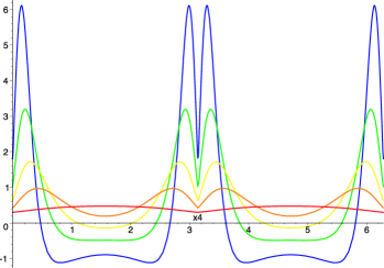
To graph them, however, we take and show these in figure 3.


Further, note that the function has a larger characteristic width, as it only converges as . This will be important when we compactify .
The height of the above functions grows as because the peak happens at a fixed value of , giving just a constant contribution times the dressing factor of . Thus, one expects the perturbative approach to be valid up to . This will be generic for later sections as well, as the decompactified behavior emerges at large in the following sections.
We also wish to characterize the width of the “spike” in each graph. One way is to make sure that variations happen on scales larger than string scale. The slope of the graphs is largest in the vicinity of the spike, and this slope is determined by its behavior, and is therefore just a constant. Therefore, the slope is simply constant. The physical length that this corresponds to, however, is , and we require that . This gives . Recalling the conditions above and , this condition follows, and so is not a new piece of information.
One may also wish to characterize the width when the linear part is no longer the dominant, and so characterize the width of when other “features” become important. This occurs when the coordinate becomes order 1, and so translates into . Again, translating this into a physical distance we find , where we have required that this distance be greater than string scale. This gives a lower bound on , however, it is the same lower bound coming from the Ricci scalar for the supergravity approximation. We see that we trust the supergravity to describe the backreaction above , and that the perturbative results are good up to .
Of course one may take the last two constraints on and turn them into a unitless constraint on the parameters. We find that this is which we can see is weaker than the other constraints , .
4.2 with compactified
Here we will examine the case with compactified as explained at the beginning of section 4. However, a few brief words are in order. We will do this case in two ways: by summing the images from the last section, and by Fourier decomposing them. These two approaches are complimentary because one expects the sum on images to converge quickly for large (when the images are well separated), and as we will see, the Fourier modes converge extremely quickly as . Further, we will be considering the antipodal embedding, , which for concreteness we parameterize by the embedding .
Sum images of Decompacitification
Looking at the Fourier transform (below), there is no problem with compactifying , however the solution for above seems to have a problem. Note that if we take the above and sum over images in for some fixed value of , we expect a divergence, as the function only converges as . However, switching back to the language, we find that the image of is
| (4.6) |
where the right hand side is it the large behavior. This, however, is actually a homogeneous solution to the original differential equation we started with. This suggests a solution to this difficulty, and we take instead
| (4.7) |
where this is just adding a zero mode of the differential equation. The sum of this function in converges, as the large behavior is order .
Now we make one more final comment. To fix , we require that
. This is roughly requiring that when you are as far away from the branes as possible that the perturbation should be 0.
The solution to this constraint is . Of course a different set of could be chosen in such a way as to not affect the sum: this, by definition, is unphysical, as none of the field values would change.
Therefore, for the compactified case, we take
| (4.8) |
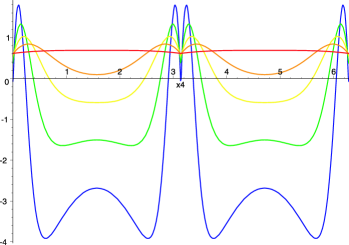
The other functions we take and simply sum on images. We plot these in figure 4.


In figure 4 we have summed many fewer modes for because this function converges very fast (as ), and so fewer images are needed. Further, we can see that one must go to much larger values of to obtain well separated features for . One could have guessed this from the results of the decompactified case: the characteristic width of the functions (associated with ) is much larger than for the other functions and . However, one can see the shape of the functions approaching the decompactified case: has a single cusp like and and have cusps like surrounded by two maxima. We show plots for various in the next subsection where we consider the Fourier transform of the equations.
Fourier decomposition
We start with the same equations as the last subsection
| (4.9) | |||
| (4.10) | |||
| (4.11) |
and Fourier transform them
| (4.12) | |||
| (4.13) | |||
| (4.14) |
where we have assumed that is periodic with
| (4.15) |
as in the last section (the reason for this parameterization is explained at the beginning of section 4).
The above equations can be brought to a simple and familiar form by the following change of coordinates and functions
The above differential equations become
| (4.16) | |||||
| (4.17) | |||||
| (4.18) |
These then are of two forms: modified Bessel equations with a simple monomial source999Solutions to these equations are known as (modified) Lommel functions. However they are related to generalized hypergeometric functions. We opt to use the notation of hypergeometric series, as these are more general, and perhaps more familiar to the reader., and an exponential function with a simple monomial source. The general solution to the above equations is [42]
| (4.19) | |||||
| (4.20) | |||||
| (4.21) |
where and are the modified Bessel functions, is the generalized hypergeometric function 101010we do in fact mean , not , and is the exponential integral function.
| (4.22) |
and we have used to remove the associated with going around the branch point at .
Here, one may worry about the convergence of the above Fourier decomposition because the coefficient above depend on in positive powers. However, recall that we wish to sum on for fixed , not fixed . In fact the factor of completely cancels out of the above coefficients once returning to the coordinate (). The only dependence comes about in the arguments of the homogeneous and non homogeneous terms. Therefore, we may effectively analyze convergence of the Fourier modes as convergence in the variable , as this is the limit to which corresponds. The inhomogeneous solution to (4.21) is indeed convergent and admits a power series expansion about . Therefore one does not wish to turn on the growing exponential (this would not converge summing on ), and the shrinking exponential is simply negligible. Hence, we may set for all m and get a convergent series.
The remaining equations, however, deserve some special treatment. The bessel equation (and the equation for ) have an essential singularity at . Therefore we consider the asymptotics of the above functions for large :
| (4.23) |
and [43]
After substituting in and choosing appropriate branches for the square roots (), one finds
| (4.25) |
We therefore use the following combinations
| (4.26) | |||
| (4.27) | |||
| (4.28) |
It is now a simple matter to replace the definition of above and sum the series. Although we offer no analytic proof here, the above functions can be seen to converge quickly enough for large . We note that because the above functions are functions of , the convergence in and are connected. As promised, the Fourier expansion converges more quickly for smaller .
In the last two equations, it should be noted that for large , the particular solution selected dominates over the remaining inhomogeneous solution. However, in the first equation, the homogeneous solution dominates. In the following, we still set .
Solving the case is trivial, but for completeness, we give the solutions for this as well
| (4.29) | |||
| (4.30) |
and we again set the unfixed constants above to 0.
We show here the plots of the physical fields for the first modes in figure 5.
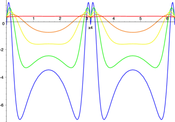
We may wish to ask what the long distance behavior is in . For this, we plot the long distance behavior of the independent modes in figure 6.


The graphs in figure 6 are directly comparable to the plots in figure 4, however there may be discrepancies between the two. For example, in figure 6 one notes that the function does not quite touch 0 at as it is required to for figure 4. This is merely a matter of setting the correct zero mode for the homogenous equation in this case. However, to make the plots match exactly in all cases, one may, if one wishes, Poisson resum the results from the last subsection, which will fix all constants above in terms of the constants from the last subsection. We, however, have not done this.
We should note also that the above analysis allows for more generality that summing the images. In the decompactification case a very specific functional form was taken, to which many homogenous solutions do not conform. This property is inherited when summing on images. By the orthogonality and completeness of the trigonometric functions, we are guaranteed to generate all solutions to the original gravitational ansatz when using the Fourier analysis.
4.3
Fourier decomposition
Fourier decomposing the general equations at the beginning of section 3 gives
| (4.31) | |||
| (4.32) | |||
| (4.33) |
where now the periodicity of
| (4.34) |
is dictated by smoothness of the gravitational solution near the tip of the cigar (). Recall that we will be considering the antipodal embedding , so that the delta functions are located at .
It is clear from the above that these functions are functions only of as is the only dimensionful parameter left. Under the coordinate change and the redefinition of fields and we find
| (4.35) | |||
| (4.36) | |||
| (4.37) |
The above differential equations are difficult to solve, even excluding the inhomogeneous piece. The homogeneous parts of the equations can be seen to have 5 regular singular points at where is a third root of unity. However, as all of the singularities are regular, one may go about finding a Laurent series expansion about any given point (using standard textbook techniques). Rather than doing this in the Fourier basis, we find that it is easier to leave the functions of intact, and expand the function about a specific value, and then solve for the functions of multiplying each power individually.
expansion
First, for expanding around the point , and to make contact with much of the literature, we change to the coordinate defined by
| (4.38) |
In these coordinates, the (non algebraic) equations read
| (4.39) | |||||
| (4.40) | |||||
| (4.41) | |||||
| (4.42) | |||||
after a bit of cleaning up.
Now, to expand about , we expand the functions multiplying each differential operator that acts on the fields above.
| (4.43) | |||||
| (4.44) | |||||
| (4.45) | |||||
| (4.46) | |||||
We will now assume that all of the Fourier modes of the above fields have expansions about with a finite number of negative powers. This allows us to simply count powers in and neglect any terms that are not of leading order. For example, this allows us to drop the term above. The rest of the equation is homogeneous in only if as . Likewise, we conclude that to leading order and . To leading order in , the above equations become
| (4.47) | |||
| (4.48) | |||
| (4.49) | |||
| (4.50) |
These are easily solved.
| (4.51) | |||||
| (4.52) | |||||
| (4.53) | |||||
| (4.54) |
where is the periodicity of defined before. Note that this is exactly the kind of behavior one would expect because when switching to “cartesian” coordinates, and is similar qualitatively to a D8 in flat space.
One may continue this process and in fact get the above functions to the next order. From the general differential equation in , one may easily read that the expansion will be in terms of odd powers of . This is because the functions being expanded are all , and so coefficients of even (odd) powers only mix with coefficients of other even (odd) powers. The next term, therefore, should be of order . We solve the resulting equations, and find
| (4.55) |
One may analyze the above functions for the various length scales of these cusps. One finds that they slope is directly limited by . This gives .
Further, the onset of new “features” is at , which we require to be a large physical length: , which is equivalent to the original condition given for the supergravity limit. Hence, we trust the supergravity approximation to describe the features near .
5 Analysis of equations: Stability
A few words are in order to explain how we will address the issue of stability. We will not solve the eigenvalue problem, numerically or otherwise, to establish the four dimensional masses for fluctuations as being positive definite with a mass gap. Instead, we will simply show that to quadratic order in fluctuations, all actions are of the form (up to gauge)
| (5.1) |
where is a field describing the fluctuation, and
| (5.2) |
This last statement is important, because it implies that anywhere the perturbative analysis is valid that (to linear order in )
| (5.3) |
The inequality holds because if the term added to the must be small. If it were not small, we would be forced to go beyond linear order in , and hence the perturbative approach would no longer be trusted. Therefore it does not change the sign of any of the functions where the perturbative analysis is valid. Hence, the action that we have written had positive definite hamiltonian
| (5.4) |
simply because it is a sum of squares.
For this reason, what seems to be important is the presence of a cancelation between the DBI and CS action at the order (we expect such terms from the solutions above).
Of course another interesting question is what happens outside of the regime of validity of the perturbative approach. This, however, is out of the scope of our present investigation, although we hope to address this in some future work.
5.1 DBI and CS equations of motion: ( solution
Of course to expand an action, we must expand about some solution to the equations of motion. For this reason, we briefly outline (and give more detail in appendix C) why ( is still a solution to the equations of motion. One may address this simply by looking at the gauge invariant information in the equations of motion: namely the cusps. The cusps in and cannot be removed with a coordinate transformations, as this would introduce delta functions into . In appendix C, we show that the cusp in , which is pure gauge, does not enter. We can read off the behavior around the cusps 111111at , similar conditions apply at to be
| (5.5) | |||||
simply by comparing the delta function source terms and the coefficient (a function of ) of the term. The next order contributions are of order because we require the functions be even about to obey the symmetry of the problem.
Now we need to find the equations of motion for the embedding functions resulting from the action
| (5.6) |
In the appendix, we show that the only interesting equation of motion is the one for , and we find that this becomes
| (5.7) | |||||
where in the third line, we ignore the higher order in corrections, as we will evaluate the derivative at . Above we have also switched back to the more familiar notation.
The term with the comes from the CS term, and may vanish for the sign choice above. We interpret this as putting a brane next to the backreacted branes. This tells that the equations of motion are satisfied for a brane placed directly on top of the other branes. If instead we had put an anti-brane, we would have found a constant force type potential, and we take that this is a solution too (although we expect an open string tachyon for small enough distances: our actions do not contain terms for strings ending on different branes).
Further, we should note that the above is a gauge independent statement. The cusps in the functions are independent of the gauge choice 121212in any sense: small coordinate transformation or shifts of by a infinitely differentiable globally exact form, and these were the only functions that contribute above (see appendix C). Therefore, the leading dependence is unaffected by small coordinate transformations. For this statement, it is important that does not appear: it’s values (cusps and all) are gauge dependent, while the other functions are determined in a gauge covariant way. Recall that while is gauge dependent, it’s cusp behavior is not: one may not remove any part of the cusp without introducing unwanted delta functions into .
This gives that to lowest order, original embedding solution is still a solution to the equations of motion. To truly consider the stability, however, we would like to know whether this extremum of the action is a maximum or a minimum. For this we will need to investigate the second order action about this point, and this will involve second derivatives in , rather than just first derivatives. Hence the even functions that we were able to ignore in the above discussion will enter.
5.2 decompactification limit
We begin with the solutions for the decompactified case in the last section
| (5.8) |
where are given in equation (4.1). We will want to construct the second order action in and so we will need to second order in . We expand the to obtain and and find
| (5.9) | |||||
where we have dropped order and higher terms.
We are now able examine stability of the decompactified limit by examining the second order action. We start by writing the pullback metric as a function of
| (5.10) |
We need the determinant of this metric to second order in , however it is easier not to expand the above metric completely, and simply realize that
| (5.11) |
where is constructed by dropping the last term in , and is the symmetric tensor defined by the last term in . Evaluating this, we find
again, dropping order and higher. We now take the expansion of the functions and evaluate to zeroth and first order in , using the above expansions about , and keeping only those terms second order in or lower.
To this we must add the term coming from the RR coupling. To do so, we recognize that
| (5.14) |
satisfies the equations of motion for the nine form potential. We use the notation to mean that the index for has been omitted. The factor of in (5.14) is constructed using only the zeroth order in metric pulled back. Further, this only has corrections of order , and so we may ignore them because of the already multiplying . Hence, to the order that we are working,
| (5.15) |
Thus, for the correct orientation of the probe brane, the term in the action completely cancels 131313We interpret this as a brane next to the backreacted brane(s), rather than an anti brane next to the backreacted brane(s)., and the total action becomes
Although we can at this point find equations of motion for the above action, and proceed with the analysis directly, we find it convenient to manipulate the above equation a bit more. For this, we note that we can redefine the coordinate as well as the field . We find it convenient to do the following transformation
| (5.17) |
(we do the coordinate change first, and then the transformation) and then for ease of notation we simply drop the from the above. Again, we may only keep order or lower in the above expansion. After doing this, we will introduce terms of the form which we integrate by parts. This affects the coefficient of . After doing so, we find that the new action is
| (5.18) | |||
The interpretation of and is that the correspond to coordinate transformations, and so are actually arbitrary and one may choose these. The numbers and are numbers that determine part of the profile of the backreaction of the branes, and so may be constrained by some physical boundary conditions. Here, however, we simply note that may be chosen to eliminate the term completely. This then leaves terms of the form times terms present when . Therefore, we conclude that when the perturbative analysis is valid, all coefficients remain the same as the case. Because of this, one may simply argue that the hamiltonian of the above action is positive definite (it is a sum of squares times positive coefficients) for the range of validity of the perturbative analysis. Hence, we conclude that in the perturbative regime, the configuration is stable.
This depended on the leading order cancelation between the DBI and coupling to the RR field. Other than this, the remaining terms were all present in the limit (up to gauge). In such a case, all corrections that are order cannot change the signs of coefficients, and so stability (in the range of validity for the perturbative approach) is preserved. We will see this again in the next section.
As a curious note, with an appropriate choice of and , one can completely cancel the leading order in contribution to the above action.
5.3 Stability of the Sakai Sugimoto model
Above, and in appendix C, we show that is still a solution to the equations of motion resulting from the DBI+CS action. To evaluate the second order action for fluctuations, we change to the radial coordinate defined by , and then to the “Cartesian” coordinates
| (5.19) |
which also allows for comparison with the analysis performed in [10]. Here the important point is that we chose the gauge , and so the only change in the plane is by a conformal factor. Hence, much of the analysis of [10] follows through. We find that the metric in these coordinates is written
| (5.20) | |||
where now all metric functions are written as functions of and , and we have defined the following functions
| (5.21) | |||||
Here we have suppressed the factor of for ease of notation, and will only reintroduce it at the end. Taking the embedding one may compute the second order action the same way as the decompactification piece. One writes the line element as where is diagonal and is already order , and so again one finds that
| (5.22) |
One may compute the DBI action easily now,
where we have defined . Further, the above function still must be expanded in . The term is the volume of the unit four sphere, and .
We will integrate the term linear in by parts, but first we find it convenient to introduce the following notation
| (5.24) | |||||
| (5.25) |
From the arguments in the last subsection, we expect the above combinations of fields to have the following behavior about
| (5.26) |
where in we ignore higher corrections in because its coefficient is already . In the above, we have determined the expansion in of order by considering the argument in the coordinates used to give equations (5.5), and then changing coordinates to the variables.
In the following, we will have to evaluate at , and henceforth, we will call this function . Similarly we define . Plugging in the above to the second order action, and reintroducing we find
where we define
| (5.28) |
as in the work of [10]. It is easy to read off the result in [10] in the limit; it is the top two lines of the right hand side. As in the last sections, we now add to this the contribution from . This is relatively easy to do, as we find
| (5.29) |
and so to second order in we can simply take
| (5.30) |
This exactly cancels the term (for the choice), as we have seen several times now (see appendix C for this occurring at the level of the equations of motion). Therefore, the full action reads
At this point it is sufficient to note that because all terms in the action were present before the perturbation, we expect that wherever the perturbative analysis is valid, the stability of the Sakai Sugimoto model is maintained. This is because whenever the perturbation is small, the above action yields a positive definite hamiltonian, and so all fluctuations will have positive energy. Further, as we have seen in the previous section, the equations admit a perturbative solution about and so the perturbative analysis is valid from up to , where for the previous sections analysis gives a good approximation to the solutions.
6 Discussion and outlook
Here we will summarize our results. From the above calculations, we can see that when u is large enough, the solutions tend to that of the decompactified case. The height of these functions all grow as and so to stay in the perturbative regime, we require that
| (6.1) |
There is a further requirement, that the supergravity approximation is valid. This gives a restriction
| (6.2) |
One may easily compare now and see which condition is more stringent, as all coefficients of and are the same. We find that generically
| (6.3) |
as we assume that is large and (see figure 7). However, we note that for small the regime of validity of the perturbative backreaction (and so the validity of the probe approximation) becomes arbitrarily large.

In figure 7, we have indicated a possible M-theory (11D SUGRA) lift, although some caution is necessary, as no know lift D8 branes is understood in the context of 11D SUGRA, at least for those described by the Romans type IIA.
We are also left with some obvious open questions:
-
1.
The topic of this paper has been the low temperature limit of the Sakai Sugimoto model, and one may wish to know the qualitative differences between the low and high temperature limits. Further, one may hope that the analysis of the high temperature limit may be easier, as the D8 branes are transverse to a cylinder, rather than a cigar.
-
2.
It would be interesting to address the backreaction of flavor branes in other brane systems using the above techniques. While one may worry about the perturbation breaking down near the brane for codimension other than 1, one may trust the cancelation between the DBI and CS terms in the quadratic action for fluctuations. We believe this to be true for the following reason: for a section of brane near a smooth point in a manifold, it’s backreaction (non perturbative contributions included) should behave just as the flat space case. In such a situation, a section of parallel probe brane near by feels no force on it because the charge and mass (per unit p volume) are the same. We may expect this to always be true. Further, in supersymmetric situations, the supersymmetry of the backreaction may be of some assistance in fixing all coefficients. We look forward to addressing these issues in some future work.
Acknowledgments
We are grateful for discussions with Oren Bergman, who was involved in the initial stages of this project. We would like to thank Ofer Aharony for discussions and comments on the draft of this paper. We also wish to thank Martha Merzig for help editing graphs, and Josh Davis for directing us to a useful reference. The work of B.B and J. S has been supported in part by the Israel Science Foundation, by a grant ( DIP H.52) of German Israel Project Cooperation D.I.P and by the European Network MRTN-CT-2004-512194.
This material is based upon work supported by the National Science Foundation under Grant No. PHY-0455649.
Appendix A Massive type IIA equations of Motion
We recall the following definitions
| (A.1) | |||||
The equations of motion for the action (2.12) are
| (A.2) | |||
| (A.3) | |||
| (A.4) | |||
| (A.5) | |||
| (A.6) | |||
| (A.7) |
where again takes values . In the above, where we have written there are indices contracted. To reintroduce the (sub)superscripts, one puts in a set of indices in the superscripts, and then puts the same indices in the same order in the subscripts. In the above, we note that is constant, and may be considered piecewise constant in the presence of sources.
Appendix B Separating the equations
Here we deal with the Einstein equations and the dilaton equation, and explain how to separate them. There are 5 Einstein equations, and one for the dilaton, and we name them
| (B.1) | |||
| (B.2) | |||
| (B.3) |
| (B.4) | |||||
| (B.5) | |||||
| (B.6) |
Each of the above equations is to be set to zero. The labeling we have used is that the subscript denotes to the equation of motion, denotes the time-time and Einstein equations (these are just one equation), denotes the equation of motion, the , the directions along the sphere, and the mixed equation. Further, we have taken to be a function only of .
We now wish to perturb the following equations about the background solution. For this purpose, we take the following expansion
| (B.7) | |||||
It is now straightforward (and rather unilluminating) to expand the equations of motion and keep only the linear term in . The only key point is that the source is already linear in and so one plugs in the background fields only to the exponential appearing with . Rather than writing this out explicitly, we will simply explain the steps involved needed to separate the equations. Henceforth when we write we mean the above equation of motion expanded to linear order in . First, the most useful equation when expanded is equation (B.6), and this becomes
| (B.8) |
This may be integrated to give
| (B.9) |
One may solve this for and plug into the other equations. We will denote doing so as . One may easily solve for now,
| (B.10) |
and so
| (B.11) |
However one can easily see that this perturbation is simply taking and linearizing on . This is because under this shift, neither nor nor is changed, and so only shifts in . The linear shift of is given by . Thus, we may safely absorb into a shift into the definition of . If need be, we may always reintroduce it by shifting equations that depend on or appropriately. Further, this is only a zero mode contribution (in ) and so will leave unaffected much of our discussion. For these reasons, we take for the time being, knowing how to reintroduce it later if need be.
At this point we have eliminated 2 equations of motion at the cost of 1 function, which puts us on course to decouple the equations.
Next, we make the simple observation that in all equations of motion only and appear. Thus, if we can solve for , we may eliminate completely. We do so by taking and solving this for . This combination still has a delta function, and so it is important at this step that is a function only of so that when the expression for is substituted into no derivatives of delta functions appear.
We have now eliminated 3 of the 6 total equations, with the remaining combinations being , , . However, here we find that
| (B.12) |
Hence, we are left with only 2 independent equations for 3 unknown functions. This appears to be under constrained, however, these equations are actually equations only of 2 linear combinations of the 3 functions. The decoupled combinations may be written
| (B.13) | |||
| (B.14) |
where
| (B.15) | |||||
| (B.16) |
We now turn to the question of fixing . For this purpose, we remember that we used the combination
| (B.17) |
to solve for . It is clear for our setup that must have some “kink” part in its solution to account for the delta function, as the only derivatives that appear act on . However, by adding a zero to the above expression, we find
| (B.18) |
Now it becomes clear how one may maintain continuity of the functions and at the same time separate the equations. We take and then solve the remaining equation above. One may have guessed this gauge, as one can bring any two dimensional metric to a conformally flat one. We do not impose this on the full metric, however, as the polynomials in are easier to work with.
One more comment is in order. If one wishes, one may linearize on a small change . Under this, and transform differently. This can give a new source term to the equation for . However, this change only affects the zero mode (in ) of , and hence will not affect the shape of in the direction.
Appendix C EOM for DBI+CS: details of solution
Here we find the equations of motion for the embedding functions resulting from the action
| (C.1) |
and explicitly show that () is still a solution. We will find the equations of motion for the first part, and then turn our attention to the second part of the above action. First, we change frame by scaling the metric to write the first part of the action
| (C.2) |
The equations of motion for the fields in the above action are
| (C.3) |
where objects with a subscript are constructed using the pullback metric, and is the full spacetime Christoffel connection. We wish to ask whether for and constant is a solution to the equations of motion. Consider first the :
where we use as shorthand for a partial derivative in , and we have used the fact that our metric is diagonal. Choosing the removes the derivative from the first part of the equation. Also, the fact that is diagonal, and identical to the pullback metric for indices , allows us to simplify the above further
| (C.5) | |||
where inside the parentheses are not summed. Note that the projects the last remaining metric down to the pullback metric, and we are left with
| (C.6) |
which simplifies further to
| (C.7) |
This is obviously zero: the metric is diagonal, so that
| (C.8) |
which then causes the first and third terms to cancel.
Hence, we are left with evaluating the equation of motion:
| (C.9) |
where we use the shorthand to mean the components.
The first term vanishes as constant. The second term we evaluate similarly to the last discussion
| (C.10) | |||||
This time, however, the and give zero (as the constant), and hence only the last term remains
where the subscripts are to denote the new frame that we switched to. Switching back to the string frame metric, we find
| (C.12) |
At this point we stop this analysis because we must also look at the equations of motion coming from the CS action, as this has a cusp as well.
First, for the embeddings that we have chosen, the background form field is the following
| (C.13) | |||||
where , producing both the positive and negative delta function. In the above, we must use only zeroth order metric functions, as the above statement is already linear in . The function is the determinant of the metric setting constant, i.e. the pullback metric on the D8s.
Next, we wish to consider the action
| (C.14) |
where the epsilon takes values . This is very easy to vary w.r.t. the fields :
Taking to be one of the directions along the world volume coordinates, we see that the first term and second term are identical. This is because in the first equation and must agree to give a non zero answer (when contracting the epsilon). Of course in the sum there are occurences of this. Hence, the cancels, and one simply gets , where we use to indicate that the index for has been omitted. The second term is also equal to this, as the contraction yields a (). Hence the full equations of motion for the fields along the volume coordinates vanish.
Next, taking the above equation of motion for the direction, one finds only a contribution from the second part, i.e.
| (C.16) |
Therefore, the full equation of motion for the field assuming that it is constant reads
| (C.17) |
where we have restored a sign earlier omitted in front of the DBI action. Also, the is to be read whether we are putting or branes in the background. Both are linear order in because to zeroth order none of the metric components depend on , and is already linear in . Hence, all other metric components are set to being their background values (except those with the derivative). Considering the cusp solution near one reads (factoring out )
| (C.18) | |||||
where in the third line, we ignore the higher order in corrections, as we will evaluate the derivative at . Above we have also switched back to the more familiar notation.
References
- [1] A. Karch and A. Katz, Adding flavor to AdS/CFT, JHEP 0206, 043 (2002); hep-th/0205236.
- [2] T. Sakai and J. Sonnenschein, Probing flavored mesons of confining gauge theories by supergravity, JHEP 0309, 047 (2003); hep-th/0305049.
- [3] J. Babington, J. Erdmenger, N. J. Evans, Z. Guralnik and I. Kirsch, Chiral symmetry breaking and pions in non-supersymmetric gauge / gravity duals, Phys. Rev. D 69, 066007 (2004); hep-th/0306018.
- [4] M. Kruczenski, D. Mateos, R. C. Myers and D. J. Winters, Towards a holographic dual of large-N(c) QCD, JHEP 0405, 041 (2004); hep-th/0311270.
- [5] S. A. Cherkis and A. Hashimoto, Supergravity solution of intersecting branes and AdS/CFT with flavor, JHEP 0211 (2002) 036 [arXiv:hep-th/0210105]; A. Karch, E. Katz and N. Weiner, Hadron masses and screening from AdS Wilson loops, Phys. Rev. Lett. 90 (2003) 091601 [arXiv:hep-th/0211107]. M. Kruczenski, D. Mateos, R. C. Myers and D. J. Winters, Meson spectroscopy in AdS/CFT with flavour, JHEP 0307, 049 (2003) [hep-th/0304032]; H. Nastase, On Dp-Dp+4 systems, QCD dual and phenomenology, hep-th/0305069; X. J. Wang and S. Hu, Intersecting branes and adding flavors to the Maldacena-Nunez background, JHEP 0309 (2003) 017; hep-th/0307218; P. Ouyang, Holomorphic D7-branes and flavored N = 1 gauge theories, Nucl. Phys. B 699 (2004) 207 [arXiv:hep-th/0311084]; C. Nunez, A. Paredes and A. V. Ramallo, Flavoring the gravity dual of N = 1 Yang-Mills with probes, JHEP 0312, 024 (2003); hep-th/0311201; S. Hong, S. Yoon and M. J. Strassler, Quarkonium from the fifth dimension, JHEP 0404 (2004) 046 [arXiv:hep-th/0312071]; N. J. Evans and J. P. Shock, Chiral dynamics from AdS space, Phys. Rev. D 70 (2004) 046002 [arXiv:hep-th/0403279]; J. L. F. Barbon, C. Hoyos, D. Mateos and R. C. Myers, The holographic life of the eta’, JHEP 0410 (2004) 029 [arXiv:hep-th/0404260]; M. Bando, T. Kugo, A. Sugamoto and S. Terunuma, Pentaquark baryons in string theory, Prog. Theor. Phys. 112 (2004) 325 [arXiv:hep-ph/0405259]; K. Ghoroku and M. Yahiro, Chiral symmetry breaking driven by dilaton, Phys. Lett. B 604 (2004) 235 [arXiv:hep-th/0408040]; J. Erdmenger and I. Kirsch, Mesons in gauge / gravity dual with large number of fundamental fields, JHEP 0412 (2004) 025 [arXiv:hep-th/0408113]; D. Arean, D. Crooks and A. V. Ramallo, Supersymmetric probes on the conifold, JHEP 0411 (2004) 035 [arXiv:hep-th/0408210]; S. Hong, S. Yoon and M. J. Strassler, On the couplings of vector mesons in AdS/QCD, arXiv:hep-th/0409118; S. Hong, S. Yoon and M. J. Strassler, Adjoint trapping: A new phenomenon at strong ’t Hooft coupling, JHEP 0603 (2006) 012 [arXiv:hep-th/0410080]; S. Kuperstein, Meson spectroscopy from holomorphic probes on the warped deformed conifold, JHEP 0503 (2005) 014 [arXiv:hep-th/0411097]; A. Paredes and P. Talavera, Multiflavour excited mesons from the fifth dimension, Nucl. Phys. B 713, 438 (2005) [arXiv:hep-th/0412260]; G. F. de Teramond and S. J. Brodsky, The hadronic spectrum of a holographic dual of QCD, Phys. Rev. Lett. 94, 201601 (2005), hep-th/0501022; S. Hong, S. Yoon and M. J. Strassler, On the couplings of the rho meson in AdS/QCD, arXiv:hep-ph/0501197; L. Da Rold and A. Pomarol, Chiral symmetry breaking from five dimensional spaces, Nucl. Phys. B 721, 79 (2005), hep-ph/0501218; K. Ghoroku, T. Sakaguchi, N. Uekusa and M. Yahiro, Flavor quark at high temperature from a holographic model, Phys. Rev. D 71 (2005) 106002 [arXiv:hep-th/0502088]; N. Evans, J. Shock and T. Waterson, D7 brane embeddings and chiral symmetry breaking, JHEP 0503 (2005) 005 [arXiv:hep-th/0502091]; I. Brevik, K. Ghoroku and A. Nakamura, Meson mass and confinement force driven by dilaton, Int. J. Mod. Phys. D 15 (2006) 57 [arXiv:hep-th/0505057]; I. Kirsch and D. Vaman, The D3/D7 background and flavor dependence of Regge trajectories, Phys. Rev. D 72, 026007 (2005) [arXiv:hep-th/0505164]; T. S. Levi and P. Ouyang, Mesons and flavor on the conifold, arXiv:hep-th/0506021; N. Mahajan, Revisiting 5D chiral symmetry breaking and holographic QCD models, Phys. Lett. B 623, 119 (2005), hep-ph/0506098; K. Ghoroku, Flavor meson localization in 5d braneworld, Phys. Lett. B 632 (2006) 405 [arXiv:hep-th/0506168]; R. Apreda, J. Erdmenger and N. Evans, Scalar effective potential for D7 brane probes which break chiral symmetry, hep-th/0509219; F. Canoura, J. D. Edelstein, L. A. P. Zayas, A. V. Ramallo and D. Vaman, Supersymmetric branes on and their field theory duals, JHEP 0603 (2006) 101 [arXiv:hep-th/0512087]; J. P. Shock, Canonical coordinates and meson spectra for scalar deformed N = 4 SYM from the AdS/CFT correspondence, arXiv:hep-th/0601025; R. Casero, C. Nunez and A. Paredes, Towards the string dual of N = 1 SQCD-like theories, arXiv:hep-th/0602027; T. Hirayama, A holographic dual of CFT with flavor on de Sitter space, arXiv:hep-th/0602258. R. Apreda, J. Erdmenger, D. Lust and C. Sieg, Adding flavour to the Polchinski-Strassler background JHEP 0701, 079 (2007) arXiv:hep-th/0610276. C. Sieg, Holographic flavour in the N = 1 Polchinski-Strassler background, JHEP 0708, 031 (2007) arXiv:0704.3544 [hep-th].
- [6] I. R. Klebanov and J. M. Maldacena, “Superconformal gauge theories and non-critical superstrings,” Int. J. Mod. Phys. A 19, 5003 (2004) [arXiv:hep-th/0409133].
- [7] F. Bigazzi, R. Casero, A. L. Cotrone, E. Kiritsis and A. Paredes, Non-critical holography and four-dimensional CFT’s with fundamentals, JHEP 0510, 012 (2005) [arXiv:hep-th/0505140].
- [8] R. Casero, A. Paredes and J. Sonnenschein, “Fundamental matter, meson spectroscopy and non-critical string / gauge JHEP 0601, 127 (2006) [arXiv:hep-th/0510110].
- [9] U. Gursoy, E. Kiritsis and F. Nitti, “Exploring improved holographic theories for QCD: Part II,” arXiv:0707.1349 [hep-th].
- [10] T. Sakai and S. Sugimoto, Low energy hadron physics in holographic QCD, Prog. Theor. Phys. 113, 843 (2005) [arXiv:hep-th/0412141].
- [11] E. Witten, Anti-de Sitter space, thermal phase transition, and confinement in gauge theories, Adv. Theor. Math. Phys. 2 (1998) 505, [arXiv:hep-th/9803131].
- [12] T. Sakai and S. Sugimoto, Prog. Theor. Phys. 114, 1083 (2006) [arXiv:hep-th/0507073].
- [13] O. Aharony, J. Sonnenschein and S. Yankielowicz, A holographic model of deconfinement and chiral symmetry restoration, Annals Phys. 322, 1420 (2007) [arXiv:hep-th/0604161].
- [14] K. Peeters, J. Sonnenschein and M. Zamaklar, Holographic melting and related properties of mesons in a quark gluon plasma, Phys. Rev. D 74, 106008 (2006) [arXiv:hep-th/0606195].
- [15] P. Kovtun, D. T. Son and A. O. Starinets, Viscosity in strongly interacting quantum field theories from black hole physics, Phys. Rev. Lett. 94, 111601 (2005) [arXiv:hep-th/0405231].
- [16] D. Mateos, R. C. Myers and R. M. Thomson, Phys. Rev. Lett. 98, 101601 (2007) [arXiv:hep-th/0610184].
- [17] A. Kehagias, New type IIB vacua and their F-theory interpretation, Phys. Lett. B 435, 337 (1998) [arXiv:hep-th/9805131].
- [18] O. Aharony, A. Fayyazuddin and J. M. Maldacena, The large N limit of N = 2,1 field theories from three-branes in F-theory, JHEP 9807, 013 (1998) [arXiv:hep-th/9806159].
- [19] M. Grana and J. Polchinski, Gauge / gravity duals with holomorphic dilaton, Phys. Rev. D 65, 126005 (2002) [arXiv:hep-th/0106014].
- [20] M. Bertolini, P. Di Vecchia, M. Frau, A. Lerda and R. Marotta, N = 2 gauge theories on systems of fractional D3/D7 branes, Nucl. Phys. B 621, 157 (2002) [arXiv:hep-th/0107057].
- [21] B. A. Burrington, J. T. Liu, L. A. Pando Zayas and D. Vaman, Holographic duals of flavored N = 1 super Yang-Mills: Beyond the probe approximation, JHEP 0502, 022 (2005) [arXiv:hep-th/0406207].
- [22] O. Aharony, E. Schreiber and J. Sonnenschein, “Stable non-supersymmetric supergravity solutions from deformations of the JHEP 0204, 011 (2002) [arXiv:hep-th/0201224].
- [23] F. Benini, F. Canoura, S. Cremonesi, C. Nunez and A. V. Ramallo, Unquenched flavors in the Klebanov-Witten model, JHEP 0702, 090 (2007) [arXiv:hep-th/0612118].
- [24] F. Benini, F. Canoura, S. Cremonesi, C. Nunez and A. V. Ramallo, Backreacting Flavors in the Klebanov-Strassler Background, arXiv:0706.1238 [hep-th].
- [25] D. Arean, A. V. Ramallo and D. Rodriguez-Gomez, Holographic flavor on the Higgs branch, JHEP 0705, 044 (2007) [arXiv:hep-th/0703094].
- [26] E. Antonyan, J. A. Harvey, S. Jensen and D. Kutasov, NJL and QCD from string theory, arXiv:hep-th/0604017.
- [27] J. L. Davis, M. Gutperle, P. Kraus and I. Sachs, Stringy NJL and Gross-Neveu models at finite density and temperature, arXiv:0708.0589 [hep-th].
- [28] L. J. Romans, Massive N=2a Supergravity In Ten-Dimensions, Phys. Lett. B 169, 374 (1986).
- [29] E. Bergshoeff, M. B. Green, G. Papadopoulos and P. K. Townsend, The IIA super-eightbrane, arXiv:hep-th/9511079.
- [30] A. Brandhuber, N. Itzhaki, J. Sonnenschein and S. Yankielowicz, Wilson loops, confinement, and phase transitions in large N gauge theories from supergravity, JHEP 9806, 001 (1998); hep-th/9803263.
- [31] Y. Kinar, E. Schreiber and J. Sonnenschein, Q anti-Q potential from strings in curved spacetime: Classical results, Nucl. Phys. B 566, 103 (2000); hep-th/9811192.
- [32] E. Bergshoeff and P. K. Townsend, Super D-branes, Nucl. Phys. B 490, 145 (1997) [arXiv:hep-th/9611173].
- [33] M. Massar and J. Troost, D0-D8-F1 in massive IIA SUGRA, Phys. Lett. B 458, 283 (1999) [arXiv:hep-th/9901136].
- [34] B. Janssen, P. Meessen and T. Ortin, The D8-brane tied up: String and brane solutions in massive type IIA supergravity, Phys. Lett. B 453, 229 (1999) [arXiv:hep-th/9901078].
- [35] A. Brandhuber and Y. Oz, The D4-D8 brane system and five dimensional fixed points, Phys. Lett. B 460, 307 (1999) [arXiv:hep-th/9905148].
- [36] M. Mihailescu, I. Y. Park and T. A. Tran, D-branes as solitons of an N = 1, D = 10 non-commutative gauge theory, Phys. Rev. D 64, 046006 (2001) [arXiv:hep-th/0011079].
- [37] E. Witten, BPS bound states of D0-D6 and D0-D8 systems in a B-field, JHEP 0204, 012 (2002) [arXiv:hep-th/0012054].
- [38] E. Bergshoeff, R. Kallosh, T. Ortin, D. Roest and A. Van Proeyen, New formulations of D = 10 supersymmetry and D8 - O8 domain walls, Class. Quant. Grav. 18, 3359 (2001) [arXiv:hep-th/0103233].
- [39] P. S. Howe, N. D. Lambert and P. C. West, A new massive type IIA supergravity from compactification, Phys. Lett. B 416, 303 (1998) [arXiv:hep-th/9707139].
- [40] D. Tsimpis, Massive IIA supergravities, JHEP 0510, 057 (2005) [arXiv:hep-th/0508214].
- [41] J. Polchinski, “String theory. Vol. 2: Superstring theory and beyond”, Cambridge, UK: Univ. Pr. (1998) 531 p
- [42] I.S. Gradshteyn, I.M. Ryzhik, ”Table of Integrals Series and Products” (pp. 1001), Fifth edition, Academic Press (1994), San Diego, CA, USA, London, UK.
- [43] The Wolfram functions site: http://functions.wolfram.com/07.22.06.0012.01